Competitive Online Optimization with Multiple Inventories: A Divide-and-Conquer Approach

Abstract.

We study a competitive online optimization problem with multiple inventories. In the problem, an online decision maker seeks to optimize the allocation of multiple capacity-limited inventories over a slotted horizon, while the allocation constraints and revenue function come online at each slot. The problem is challenging as we need to allocate limited inventories under adversarial revenue functions and allocation constraints, while our decisions are coupled among multiple inventories and different slots. We propose a divide-and-conquer approach that allows us to decompose the problem into several single inventory problems and solve it in a two-step manner with almost no optimality loss in terms of competitive ratio (CR). Our approach provides new angles, insights and results to the problem, which differs from the widely-adopted primal-and-dual framework. Specifically, when the gradients of the revenue functions are bounded in a positive range, we show that our approach can achieve a tight CR that is optimal when the number of inventories is small, which is better than all existing ones. For an arbitrary number of inventories, the CR we achieve is within an additive constant of one to a lower bound of the best possible CR among all online algorithms for the problem. We further characterize a general condition for generalizing our approach to different applications. For example, for a generalized one-way trading problem with price elasticity, where no previous results are available, our approach obtains an online algorithm that achieves the optimal CR up to a constant factor.

1. Introduction

Competitive online optimization is a fundamental tool for decision making with uncertainty. We have witnessed its wide applications spreading from EV charging (zhao2017robust, ; alinia2018competitive, ; lin2021minimizing, ; wang2018electrical, ), micro-grid operations (lu2013online, ; zhang2016peak, ), energy storage scheduling (mo2021eEnergy, ; mo2021infocom, ) to data center provisioning (lin2012dynamic, ; lu2012simple, ), network optimization (shi2018competitive, ; guo2018joint, ), and beyond. Theoretically, there are multiple paradigms of general interest in the online optimization literature. Typical examples include the online covering and packing problem (buchbinder2009design, ), online matching (TCS-allocation, ), online knapsack packing (zhou2008budget, ), one-way trading problem (el2001optimal, ), and online optimization with switching cost (lin2012online, ; bansal20152, ).

Among these applications and paradigms, we focus on optimizing the allocation of limited resources, like inventories, budgets, or power, across a multi-round decision period with dynamic per-round revenues and allocation conditions. For example, in online ads display platform (e.g., google search), the operator allocates display slots to multiple advertisers (cf. inventories) with contracts on the maximum number (cf. capacity) of impressions (Feldman2009Online, ). At each round, the real-time search reveals the number of total available display slots and interesting slots for each advertiser (cf. allocation constraint). It also reveals the payoff of each advertiser from impressions at the display slots (cf. revenue function). The revenue of an advertiser relies on the number of obtained impressions and the quality of each impression relating to dynamic factors like the click rate and engagement rate (Devanur2012Concave, ).

The above observations motivate us to study the important paradigm – competitive online optimization problem under multiple inventories (OOIC-M), where a decision-maker with multiple inventories of fixed capacities seeks to maximize the per-round separable revenue function by optimizing the inventory allocation at each round. The decision maker further faces two allocation constraints at each round, the allowance constraint that limits the total allocation of different inventories at the round and the rate constraint that limits the allocation of each inventory at the round. The problem has two main challenges. First, as in online optimization under (single) inventory constraints  (cr_pursuit2018, ; Sun2020Competitive, ), the decision-maker does not have access to future revenue functions, while the limited capacity of each inventory coupling the online decisions regarding each inventory across time. Second, the allocation constraints that couples the allocation decisions across the multiple inventories at each round. The combination of allowance constraint and rate limit constraint appears frequently and is with known challenges in online matching and allocation problems (azar2006maximizing, ; KALYANASUNDARAM20003bmatching, ; TCS-allocation, ; Deng2018Capacity, ).

In the literature, the authors in (ma2020algorithms, ; Sun2020Competitive, ) tackle the problem using the well-established online primal-and-dual framework (buchbinder2009design, ; Devanur2013Randomized, ; niazadeh2013unified, ). They design a threshold function for each inventory with regard to the allocated amount, which can be view as the marginal cost of the inventory. They then greedily allocate the inventory at each round by maximizing the pseudo-revenue function defined by the difference between the revenue function and the threshold function. In contrast, we propose, in this paper, a divide-and-conquer approach to the online optimization with multiple inventories. Our approach is novel and provides additional insights to the problem. It allows us to separate the two challenges of the problem, 1) the online allocation for each inventory subject to the limited inventory capacity and unknown future revenue functions, and 2) the coupled allocation among multiple inventories due to the allowance constraint at each round. In the following, we summarize our contributions.

First, in Sec. 4, we generalize the CR-Pursuit($\pi$) algorithm (cr_pursuit2018, ) to tackle the single inventory case, OOIC-S, which is an important component in our divide-and-conquer approach. We show that it achieves the optimal competitive ratio (CR) among all online algorithm for OOIC-S.

Second, in Sec. 5, we propose a divide-and-conquer approach to design online algorithms for online optimization under multiple inventories and dynamic allocation constraints. By adding an allowance allocation step, we decompose the multiple inventory problem into several single inventory problems with a small optimality loss in terms of CR. We show that when the revenue functions have bounded gradients, the CR achieved by our algorithm is optimal at a small number of inventories and within an additive constant to the lower bound of the best possible CR among all online algorithms for the problem at an arbitrary number of inventories.

Third, in Sec. 6, we discuss generalizations of our proposed approach to broader classes of revenue functions. We provide a sufficient condition for applying our online algorithm and derive the corresponding CR it can achieve. For example, we consider revenue functions capturing the one-way trading problem with price elasticity, where only the results on single inventory case are available in existing literature (Sun2020Competitive, ; cr_pursuit2018, ). We show that our approach obtains an online algorithm that achieves the optimal CR up to a constant factor.

Finally, our results in Sec. 5.2.2 generalize the online allocation maximization problem in (azar2006maximizing, ) and the online allocation with free disposal problem in (Feldman2009Online, ) by admitting allowance augmentation in online algorithms, which is of independent interest. We show that we can improve the CR from $\frac{e}{e-1}$ to $\frac{1}{\pi}\cdot\frac{e^{\frac{1}{\pi}}}{e^{\frac{1}{\pi}}-1}$, when our online algorithms are endowed with $\pi$-time augmentation in allowance and allocation rate at each round.

2. Related Work

	Model	Existing results		Our result§
Single	Linear	$\ln\theta+1^{\star}$	(lorenz2009optimal, ; Sun2020Competitive, ; el2001optimal, ; cr_pursuit2018, )	$\ln\theta+1^{\star}$
	Concave†	$\ln\theta+1^{\star}$	(Sun2020Competitive, )	$\ln\theta+1^{\star}$
Multi	$\theta=1$	$e/(e-1)^{\star}$	(karp1990optimal, ; Devanur2013Randomized, ; KALYANASUNDARAM20003bmatching, )	$e/(e-1)^{\star}$
	Concave†	$<\ln\theta+2$	(Sun2020Competitive, ; ma2020algorithms, )	$<\ln\theta+2$, if $\ln\theta+1<N$
				$\ln\theta+1^{\star}$, otherwise
	Concave‡	None		$\Omega({\ln\theta})$

$\theta$ is a parameter representing the level of the input uncertainty. $N$ is the number of inventories.
$\mathsection$: We propose a divide-and-conquer approach while existing work mostly base on primal-and-dual framework (buchbinder2009design, ).
^†: Concave revenue function with bounded gradients. ^‡: Concave revenue function with price elasticity (See Sec. 6).
^⋆: The result is optimal.

Table 1. Comparison of our work and existing studies for online optimization under inventory constraints.

We focus on the competitive online optimization problem with multiple inventories and dynamic allocation constraints. Our problem generalizes a couple of well-studied online problems, including the one-way trading problem (el2001optimal, ), the online optimization under a single inventory constraint (cr_pursuit2018, ; Sun2020Competitive, ), and the online fractional matching problem (KALYANASUNDARAM20003bmatching, ; azar2006maximizing, ). Our results also reproduce the optimal CR under such settings. Our problem is studied in  (Sun2020Competitive, ), and a discrete counterpart is studied in (ma2020algorithms, ). Compared with the existing study, we propose a novel divide-and-conquer approach. We show that our approach achieves a close-to-optimal CR, which notably matches the lower bound when the number of inventories is relatively small. We summarize the related literature on online optimization under inventory constraints in Table 1.

Our problem also covers a fractional version of online ads display problem (TCS-allocation, ), which is an online matching problem with vertex capacity and edge value. No positive result is possible when the value is unbounded (Feldman2009Online, ). In (Feldman2009Online, ), the authors consider a model of “free disposal”, i.e., the online decision maker can remove the past allocated edge without any cost (but can not re-choose the past edge). Here, we instead consider the case that the values of all edges are bounded in a pre-known positive range and no removable on past decision is available. We are interested in how the CR of an online algorithm behaviors with regard to the uncertain range of value. Interestingly, by our divide-and-conquer approach, we can extend the results in the “free disposal” model to the irremovable setting. Also, we provide additional insight and results to the problem when considering an online augmentation scenario that the online decision maker is with larger allowance and allocation rate at each round; see more details in 5.2.2.

Another related problem is online knapsack packing problem (zhou2008budget, ). In the problem, items are associated with weight and value and come online. An online decision maker with a capacity limited knapsack determines whether to pack the item at its arrival to maximize the total value while guaranteeing that the total weight would not exceed the capacity. A single knapsack problem with infinitesimal assumption is studied in (zhou2008budget, ) with the application on key-work bidding. It can be viewed as a special case of the one-way trading problem (Sun2020Competitive, ), which is covered by the online optimization problem with a single inventory (cr_pursuit2018, ). The fractional multiple knapsack packing problem with unit weight is studied in (Sun2020Competitive, ), where the decision maker can pack any fraction of the item instead of $0/1$ decision. Our problem is also related to the online packing problem (buchbinder2009design, ; azar2016online, ) where the authors consider general packing constraints. Here, we focus on specific inventory constraints and allocation constraints.

3. Problem Formulation

In the section, we formulate the optimal allocation problem with multiple inventories. We discuss the practical online scenario and the performance metric for online algorithms. We further discuss the state-of-the-art to the problem. We summarize the important notions in Table 2.

Table 2. Notation Table.

Notation	Meaning
$g_{i,t}(\cdot)$	Revenue function of inventory $i$ at slot $t$
$v_{i,t}$	Allocation of inventory $i$ at slot $t$
$C_{i}$	Capacity of inventory $i$
$A_{t}$	Allowance of total allocation among all inventories at slot $t$
$\delta_{i,t}$	The maximum allocation of inventory $i$ at slot $t$
$\theta$	$\theta=p_{\max}/p_{\min}$, where $[p_{\min},p_{\max}]$ is the range of the gradient of revenue functions
$\hat{a}_{i,t}$	Online allowance allocation to inventory $i$ at slot $t$
$\hat{v}_{i,t}$	Online inventory allocation of inventory $i$ at slot $t$
$\eta_{i,t}$	Online revenue of inventory $i$ up to slot $t$
$\tilde{OPT}_{i,t}$	Optimal objective of OOIC-Mi given allowance allocations    and revenue functions up to slot $t$
$OPT_{t}$	Optimal offline total revenue of OOIC-M up to slot $t$
$\Phi(\pi)$	Maximum total online allocation of CR-Pursuit($\pi$)

3.1. Problem Formulation

We consider $N$ inventories, and a decision period with $T$ slots. We denote the capacity of inventory $i$ as $C_{i}$. At each slot $t\in[T]$, each inventory $i$ is associated with a revenue function $g_{i,t}(v_{i,t})$, which represents the revenue of allocating an amount of $v_{i,t}$ inventory $i$ at slot $t$. However, at each slot $t\in[T]$, we are restricted to allocate at most $\delta_{i,t}$ of inventory $i$, and the total allocation of all inventories at each slot $t$ is bounded by the allowance $A_{t}$. Our goal is to find an optimal allocation scheme that maximizes the total revenue in the decision period, while satisfying the allocation restrictions.

Overall, we consider the following problem,

(1) $$\textsf{OOIC-M}:\;\max\quad \sum_{i\in[N]}{\sum_{t\in[T]}{g_{i,t}(v_{i,t})}}$$

(2) s.t. $$\sum_{t}v_{i,t}\leq C_{i},\forall i\in[N],$$

(3) $$\sum_{i}v_{i,t}\leq A_{t},\forall t\in[T],$$

(4) $$0\leq v_{i,t}\leq\delta_{i,t},\forall t\in[T],i\in[N],$$

In OOIC-M, we optimize the inventory allocation $\{v_{i,t}\}_{i\in[N],t\in[T]}$ to achieve the maximum total revenue subjecting to the capacity constraint of each inventory  (2), the allowance constraint at each slot (3), and the allocation rate limit constraint for each inventory at each slot (4). Without loss of generality, we assume that $\delta_{i,t}\leq A_{t},\forall i,t$. We consider the following set of revenue functions, denoted as $\mathcal{G}$,

• $g_{i,t}(\cdot)$ is concave and differentiable with $g(0)=0$;

• $g_{i,t}^{\prime}(v_{i,t})\in[p_{\min},p_{\max}],\forall v_{i,t}\in[0,\delta_{i,t}]$.

We consider that $p_{\max}\geq p_{\min}>0$ and denote $\theta=p_{\max}/p_{\min}$. The revenue functions capture the case where the marginal revenue of allocating more inventory is non-increasing in the allocation amount but always between $p_{\min}$ and $p_{\max}$. We also discuss how we can apply our approach to different sets of revenue functions with corresponding applications in Sec 6.

In the offline setting, the problem input is known in advance, and OOIC-M is a convex optimization problem with efficient optimal algorithms. However, in practice, we are facing an online setting as we describe next.

3.2. Online Scenario and Performance Metric

In the online setting, we consider that the pre-known problem parameters include the class of revenue function $\mathcal{G}$ and corresponding range $[p_{\min},p_{\max}]$, the number of inventories $N$, and the capacity of each inventory $\{C_{i}\}_{i\in[N]}$. Other problem parameters are revealed sequentially. More specifically, at each slot $t$, the online decision maker without the information of the decision period $T$ is fed the revenue functions $\{g_{i,v}(\cdot)\}_{i\in[N]}$, the allowance $A_{t}$ and the allocation limits $\{\delta_{i,t}\}_{i\in[N]}$. We needs to irrevocably determine the allocation at slot $t$, i.e., $\{v_{i,t}\}_{i\in[N]}$. After that, if the decision period ends, we stop and know the information of $T$. Otherwise, we move to next slot and continue the allocation. We denote a possible input as

(5) $$\sigma=\left(T,\{g_{i,t}(\cdot)\}_{i\in[N],t\in[T]},\{A_{t}\}_{t\in[T]},\{\delta_{i,t}\}_{i\in[N],t\in[T]}\right)$$

We use the CR as a performance metric for online algorithms. The CR of an algorithm $\mathcal{A}$ is defined as,

(6) $$\mathcal{CR(A)}=\sup_{\sigma\in\Sigma}\frac{OPT(\sigma)}{ALG(\sigma)},$$

where $\sigma$ denotes an input, $OPT(\sigma)$ and $ALG(\sigma)$ denote the offline optimal objective and the online objective applying $\mathcal{A}$ under input $\sigma$, respectively. We use $\Sigma$ to represent all possible input we are interested in. Specifically,

(7) $$\Sigma\triangleq\{\sigma\left|T\in\mathbb{Z}^{+},g_{i,t}(\cdot)\in\mathcal{G},A_{t}\geq 0,\delta_{i,t}\geq 0,\forall i\in[N],t\in[T]\right.\},$$

In competitive analysis, we focus on the worst-case guarantee of an online algorithm, which is defined by the maximum performance ratio between the offline optimal and the online objective of the algorithm. In the online setting, we are facing two main challenges, 1) the decision maker does not known the future revenue functions, while the allocation now would affect the future decision due to the capacity constraint (cr_pursuit2018, ); and 2) the online allowance constraints and rate constrains couple the decisions across the inventories, which are with known challenges in online matching and allocation problems (KALYANASUNDARAM20003bmatching, ; TCS-allocation, ).

3.3. State of the Art

The online problem has been studied in  (Sun2020Competitive, ) under the same revenue function set $\mathcal{G}$. A discrete counterpart of the problem is studied in (ma2020algorithms, ). In some special cases, our revenue functions cover the linear functions with slopes between $[p_{\min},p_{\max}]$. In addition, when $p_{\max}=p_{\min}$, our problem reduces to maximizing the total amount of allocation, which has been widely studied in (azar2006maximizing, ; Deng2018Capacity, ; karp1990optimal, ; Devanur2013Randomized, ; KALYANASUNDARAM20003bmatching, ). Here, we introduce a novel divide-and-conquer approach for the problem and show the our approach can achieve a close-to-optimal CR. In Sec. 6, we also show that our approach can be applied to different sets of revenue functions, which have not been studied in the existing literature.

Before proceeding, we discuss the two most relevant works, namely (ma2020algorithms, ) and  (Sun2020Competitive, ) in the literature. They both apply the online primal-dual analysis and design threshold functions for the online decision-makings of OOIC-M. While the work (ma2020algorithms, ) studied a discrete setting differing from the continuous setting studied in (Sun2020Competitive, ) and our work, it is known in (niazadeh2013unified, ) that the same threshold-based function can be directly applied to the continuous setting, attaining the same CR. In the following, let us reproduce the algorithm for the continuous setting and the CR achieved by (ma2020algorithms, ). The CR is better than the one proposed in (Sun2020Competitive, ), and thus we deem it as the state of the art in the literature. We also compare the CR they achieve and ours in Sec. 5; see an illustration example in Fig. 2.

Let $\phi_{i}(w)$ denote the threshold function for each inventory $i$, where $w$ refers to the amount of allocated capacity of the inventory and $\phi_{i}(w)$ can be viewed as a pseudo-cost of the allocation. At each slot, the algorithm determines the allocated amount $v_{i,t}$ of inventory $i$ at slot $t$ by maximizing the per-round pseudo-revenue, which is the difference between the revenue and the threshold function, i.e.,

(8) $$\textsf{(P\&D):}\;\max\quad \sum_{i\in[N]}\left({g_{i,t}(v_{i,t})}-\int_{w_{i,t-1}}^{w_{i,t-1}+v_{i,t}}\phi_{i}(w)dw\right)$$

(9) s.t. $$\sum_{i}v_{i,t}\leq A_{t},$$

(10) $$0\leq v_{i,t}\leq\delta_{i,t},\forall i\in[N],$$

where $w_{i,t-1}$ is the total online allocation of inventory $i$ from the first slot to slot $t-1$. The algorithm is proposed in (Sun2020Competitive, ), which can be viewed as a continuous reinterpretation of the discrete algorithm in (ma2020algorithms, ). According to Appendix E of (ma2020algorithms, ), we can apply the following threshold function given that the gradient of $g_{i,t}(v_{i,t})$ is uniformly bounded in range $[p_{\min},p_{\max}]$,

(11) $$\phi_{i}(w)=\begin{cases}(p_{\min})^{\frac{1-w/C_{i}}{1-\chi}}(p_{\max})^{\frac{w/C_{i}}{1-\chi}},&w\in[0,\chi\cdot C_{i}];\\ p_{\min}\cdot\frac{e^{w/C_{i}}-1}{e^{\chi}-1},&w\in[\chi\cdot C_{i},C_{i}];\end{cases}$$

where $\chi={W(\ln(\theta)\cdot e^{\ln(\theta)-1})-\ln\theta+1}$ ($W(\cdot)$ is the Lambert-W function).

Proposition 1 ((ma2020algorithms, )).

With the threshold function (11), the threshold-based algorithm can achieve a competitive ratio of

(12) $$\tilde{\chi}=\frac{1}{1-e^{-\chi}}.$$

We provide the proof in Appendix A. We note that the proofs in (Sun2020Competitive, ) and (ma2020algorithms, ) follow similar ideas based on the online primal-dual framework but are different in presentations as one is discussing in the continuous setting (Sun2020Competitive, ) and the other in the discrete setting (ma2020algorithms, ). As we are considering the continuous setting, our proof follows the same presentation discussed in (Sun2020Competitive, ) and applies the properties of the threshold function (11) discussed in (ma2020algorithms, ).

4. CR-Pursuit for Single Inventory Problem

In this section, we first discuss the problem with single inventory. We extend the CR-Pursuit in (cr_pursuit2018, ) to cover the rate limit constraint and provide additional insights that will facilitate our algorithm design under the multiple inventories case.

In the single inventory case, OOIC-M is reduced to the following problem,

(13) $$\textsf{{{OOIC-S}}}:\;\max \sum_{t}g_{t}(v_{t})$$

(14) s.t. $$\sum_{t}v_{t}\leq C$$

(15) var. $$0\leq v_{t}\leq\delta_{t},\forall t,$$

where $C$ denotes the capacity of the inventory, $g_{t}(v_{t})$ represents the revenue of allocating $v_{t}$ quantity of inventory at slot $t$, and $\delta_{t}$ is the rate limit restricting the maximum allocation at slot $t$. The goal is still to maximize the total revenue by determining the inventory allocation $v_{t}$ at each slot. We focus on the online setting described in Sec. 3.2 with $N$ specified to be one. We note that the OOIC-S has been studied in (Sun2020Competitive, ). Also, the case under different assumptions on revenue functions and without rate limit has also been studied in (cr_pursuit2018, ).

Here, we generalize the results in (cr_pursuit2018, ) to consider revenue function set $\mathcal{G}$ and involve rate limit constraint. The online algorithm CR-Pursuit($\pi$), proposed in (cr_pursuit2018, ), is a single-parametric online algorithm with $\pi$ as the parameter. At slot $t$, the algorithm first computes the optimal value of OOIC-S given the input revenue functions and rate limits up to $t$, which we denote as $OPT_{S}(t)$. It then determines the allocation $\hat{v}_{t}$ at slot $t$ such that

(16) $$g_{t}(\hat{v}_{t})=\frac{1}{\pi}\left(OPT_{S}(t)-OPT_{S}(t-1)\right).$$

Under CR-Pursuit($\pi$), we define the maximum total allocation of the algorithm,

(17) $$\Phi(\pi)\triangleq\sup_{\sigma\in\Sigma}\sum_{t}{\hat{v}_{t}},$$

where $\hat{v}_{t}$ is determined by (16). By design, we clearly have the following properties of the CR-Pursuit($\pi$) algorithm.

Lemma 2.

We have $\hat{v}_{t}\leq\frac{1}{\pi}\cdot\delta_{t}$.

Proof.

As $g_{t}(v_{t})$ is increasing and concave function, and

(18) $$g_{t}(\hat{v}_{t})=\frac{1}{\pi}\left(OPT_{S}(t)-OPT_{S}(t-1)\right)\leq\frac{1}{\pi}\cdot g_{t}(\delta_{t})$$

We have $\hat{v}_{t}\leq\frac{1}{\pi}\cdot\delta_{t}$. ∎

Lemma 3 shows a upper bound on the online allocation, which guarantees the existence of $\hat{v}_{t}$ at each slot. It will also be useful for our algorithm design and CR analysis for OOIC-M, which we will discuss in Sec. 5.

Lemma 3.

CR-Pursuit($\pi$)is feasible and $\pi$-competitive for OOIC-S if $\Phi(\pi)\leq C$.

Proof.

Considering an arbitrary input $\sigma$, we first note that it is clear that $\hat{v}_{t}\leq\delta_{t}$ according to Lemma 2. Then if $\Phi(\pi)\leq C$, we have $\sum_{t}\hat{v}_{t}\leq C$, i.e., it satisfies the inventory constraint under input $\sigma$.

Summarizing (16) over all $t$, we have, the online objective

(19) $$ALG(\sigma)=\sum_{t=1}^{T}g_{t}(\hat{v}_{t})=\frac{1}{\pi}OPT_{S}(T)=\frac{1}{\pi}\cdot OPT_{S}(\sigma),$$

where $OPT_{S}(\sigma)$ is the optimal offline objective. Thus the algorithm is $\pi$-competitive.

∎

Lemma 3 shows that we can rely on characterizing $\Phi(\pi)$ to optimize the choice of $\pi$ in CR-Pursuit($\pi$). Further, we can interpret $\Phi(\pi)$ as the inventory the online algorithm CR-Pursuit($\pi$) needs to maintain $\pi$-competitive. For example, suppose for an online algorithm, we now can utilize $\Phi(1)$ capacity of the inventory while the capacity of the offline optimal remains $C$. Then we can run CR-Pursuit(1) and achieve that same performance as the offline optimal, i.e., 1-competitive.

We have the following results on the upper bound on $\Phi(\pi)$.

Lemma 4.

We have

(20) $$\Phi(\pi)\leq\frac{\ln\theta+1}{\pi}\cdot C$$

We summarize the proof idea of Lemma 4 here while leaving the detailed proof to Appendix B. We first notice that a more general results in (cr_pursuit2018, ) can be extended to the case with rate limit constraint, as shown in Proposition 15 in Appendix B. Although the results in (cr_pursuit2018, ) do not cover the revenue functions we consider here, it covers the revenue functions in the maximizer of $\Phi(\pi)$ as special cases. This observation leads to Lemma 4.

According to the above discussion, we can provide the competitive analysis of CR-Pursuit($\pi$)  for OOIC-S.

Theorem 5.

For OOIC-S, CR-Pursuit($\pi_{1}$) is $\pi_{1}$-competitive, where $\pi_{1}=\ln\theta+1$. And, it is optimal among all online algorithms for the problem.

According to Lemma 3 and Lemma 4, it is clear that CR-Pursuit($\pi_{1}$) is feasible and $\pi_{1}$-competitive. Further, according to the results in (cr_pursuit2018, ; Sun2020Competitive, ), we know that $\ln\theta+1$ is the lower bound or the optimal CR to OOIC-S. Thus, CR-Pursuit($\pi_{1}$) is also optimal.

5. Online Algorithms for Multiple Inventory Problem

In this section, we introduce our divide-and-conquer online algorithm A&P($\pi$) for OOIC-M, where $\pi$ is a parameter to be specified. We first outline the algorithm structure. Following the structure, we then propose our general online algorithm for arbitrary $N$. We next show a simple and optimal online algorithm when $N$ is relatively small. Finally, we summarize our algorithm and provide the competitive analysis. An illustration of our approach and results is shown in Fig 1.

5.1. Algorithm structure

We consider a divide-and-conquer approach for deriving online algorithms for OOIC-M. The general idea is that we can optimize OOIC-M  by first allocating the allowance at each slot to the inventories and then separately optimizing the allocation of each inventory given the allocated allowance. More specifically, we define the following subproblem for each $i\in[N]$,

(21) $$\textsf{${\textsf{OOIC-M}_{i}}$}:\;\max \sum_{t}\tilde{g}_{i,t}(v_{i,t})$$

(22) $$s.t. \sum_{t}v_{i,t}\leq C_{i}$$

(23) $$0\leq v_{i,t}\leq a_{i,t},\forall t,$$

where $a_{i,t}$ is the allocated allowance to user $i$ at slot $t$. $\tilde{g}_{i,t}(v_{i,t})$ is another algorithmic design space that allows us to exploit the online augmentation scenario when allocating the allowance allocation in Sec. 5.2.2. Under the offline setting, we note that such a decomposition is of no optimality loss. For example, we can choose $\tilde{g}_{i,t}(v_{i,t})=g_{i,t}(v_{i,t})$ and set the allowance allocation $a_{i,t}=v^{*}_{i,t}$ for all $i$ and $t$, where ${\{v^{*}_{i,t}\}}_{i\in[N],t\in[T]}$ is the offline optimal solution of OOIC-M. Then, optimizing the subproblems separately given the allowances would reproduce the offline optimal solution.

Following this structure, we can design an online algorithm that mainly consists of two steps at each slot $t$,

1. Step-I: Determine the allowance allocation, $\{\hat{a}_{i,t}\}_{i\in[N]}$, irrevocably.

2. Step-II: Determine the the inventory allocation for each online ${\textsf{OOIC-M}_{i}}$, $\{\hat{v}_{i,t}\}_{i\in[N]}$, irrevocably.

We note that this divide-and-conquer approach allows us to separately tackle the two main challenges of the problem. First, the revenue functions come online while the allocation across the decision period is coupled due to the capacity constraint for each inventory, which is mainly handled by Step-II. Second, the online allowance constraints and the rate constraints couple the decisions across the inventories, which we tackle in Step-I. We can directly apply $\{\hat{v}_{i,t}\}_{t\in[T]}$ as the output of an online algorithm for each inventory $i$. We can view the Step-II as solving ${\textsf{OOIC-M}_{i}}$ in an online manner. More specifically, at each $t$, for each $i$, we observe input $\hat{a}_{i,t}$ (determined at Step-I) and $\tilde{g}_{i,t}(\cdot)$, and need to determine $v_{i,t}$ irrevocably. In terms of feasibility, an immediate advantage is that, it satisfies the inventory constraint (2) if it is a feasible solution to ${\textsf{OOIC-M}_{i}}$. However, we need further care to make sure the satisfaction of the allowance constraint (3) and allocation rate limit (4). As for performance guarantees, we can first analyze the performance of the each step and then combine them to show the overall competitive analysis. In the following, we will discuss how the proposed online algorithm behaviors at both steps to ensure the feasibility and achieve a close-to-optimal CR.

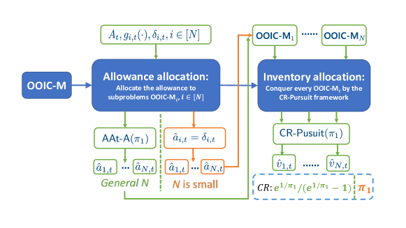
Figure 1. An Illustration of Our Divide-and-Conquer Approach and Results.

5.2. The A&P_l($\pi$) Algorithm for General $N$

In this subsection, we will propose an online algorithm for general number of inventories following the divide-and-conquer structure discussed in Sec. 5.1. We denote the algorithm as A&P_l($\pi$), where $\pi$ is parameter to be specified. In the following, we first introduce the Step-II of A&P_l($\pi$), determining the allocation of OOIC-M_i given the allowance from Step-I. We then introduce Step-I, determining the allowance of each inventories. We denote the allocated allowance from Step-I as $\hat{a}_{i,t},\forall i,t$.

5.2.1. Step-II of A&P_l($\pi$)

In this step, A&P_l($\pi$) determines the online inventory allocation for each ${\textsf{OOIC-M}_{i}}$ given the allocated allowance (denoted as $\{\hat{a}_{i,t}\}_{i\in[N]}$) from Step-I.

In Step-II of A&P_l($\pi$), it sets

(24) $$\tilde{g}_{i,t}(v_{i,t})=\pi\cdot g_{i,t}(\frac{v_{i,t}}{\pi}).$$

We denote the optimal objective of ${\textsf{OOIC-M}_{i}}$ given its input up to slot $t$ as $\tilde{OPT}_{i,t}$. We set $\tilde{OPT}_{i,0}=0$. At each slot $t$, it determines the allocation $\hat{v}_{i,t}$ such that it satisfies

(25) $$g_{i,t}(\hat{v}_{i,t})=\frac{1}{\pi}\left(\tilde{OPT}_{i,t}-\tilde{OPT}_{i,t-1}\right).$$

While it looks similar to the CR-Pursuit($\pi$) algorithm discussed in Sec. 4 and (cr_pursuit2018, ), we note that a major difference is that we are using the original revenue function $g_{i,t}(\cdot)$ to pursuit a fraction of $1/\pi$ of the optimal objective achieved over the revenue function $\tilde{g}_{i,t}$ instead of $g_{i,t}(\cdot)$. In general, $\tilde{g}_{i,t}$ defined in (24) is no less than $g_{i,t}(\cdot)$ (take equality under the linear function case). Thus, it may be more difficult for the Step-II to achieve the same performance ratio ($\pi_{1}$) between the optimal objective to the online objective for each ${\textsf{OOIC-M}_{i}}$ as that in Sec. 4. However, we would show the performance ratio remains achievable in Lemma 7. The design of $\tilde{g}_{i,t}(\cdot)$ is important for achieving a better approximation ratio between the total optimal objective of the subproblems and the optimal objective of OOIC-M, which we would discuss in Step-I, Sec. 5.2.2.

To analyze Step-II, we first propose the following proposition on the properties of the online allocation $\hat{v}_{i,t},\forall i,t$.

Lemma 6.

We have $\hat{v}_{i,t}\leq\frac{1}{\pi}\cdot\hat{a}_{i,t},\forall i,t$.

Proof.

We have

(26) $$g_{i,t}(\hat{v}_{i,t})=\frac{1}{\pi}\left(\tilde{OPT}_{i,t}-\tilde{OPT}_{i,t-1}\right)\leq\frac{1}{\pi}\cdot\pi\cdot g_{i,t}(\frac{\hat{a}_{i,t}}{\pi})\leq g_{i,t}(\frac{\hat{a}_{i,t}}{\pi})$$

Thus, as $g_{i,t}(\cdot)$ is increasing, we conclude $\hat{v}_{i,t}\leq\frac{1}{\pi}\cdot\hat{a}_{i,t}$. ∎

While this is a simple observation on the online solution, it plays an important role on designing the allowance allocation in Step-I, Sec. 5.2.2 and improving the overall performance of our online algorithm A&P_l($\pi$) for OOIC-M.

We denote the objective value of the online solution to OOIC-M_i at slot $t$ as $\eta_{i,t}$,

(27) $$\eta_{i,t}\triangleq\sum_{\tau=1}^{t}g_{i,\tau}(\hat{v}_{i,\tau})$$

We provide performance analysis of Step-II in the following lemma. Recall that $\pi_{1}=\ln\theta+1$.

Lemma 7.

We have that for each $i\in[N]$, Step-II of A&P($\pi_{1}$) always produces a feasible solution to ${\textsf{OOIC-M}_{i}}$, and for any slot $t$, the online objective

(28) $$\eta_{i,t}\geq\frac{1}{\pi_{1}}\cdot\tilde{OPT}_{i,t}.$$

Proof.

The performance guarantee in (28) is simply implied by (25) when choosing $\pi=\pi_{1}$.

We now show the feasibility. We note that, when choosing $\pi=\pi_{1}$, ${\textsf{OOIC-M}_{i}}$ with $\tilde{g}_{i,t}(\cdot)$ determined by (24) and a factor of $\frac{1}{\pi_{1}}$ in objective value is equivalent to

(29) $$\textsf{R-${\textsf{OOIC-M}_{i}}$}:\;\max \sum_{t}g_{i,t}(z_{i,t})$$

(30) $$s.t. \sum_{t}z_{i,t}\leq\frac{C_{i}}{\pi_{1}}$$

(31) $$0\leq z_{i,t}\leq\frac{\hat{a}_{i,t}}{\pi_{1}},\forall t$$

, where $z_{i,t}\triangleq v_{i,t}/\pi_{1}$. Then, determining the online allocation according to (25) is equivalent to find $\hat{v}_{i,t}$ such that

(32) $$g_{i,t}(\hat{v}_{i,t})=\hat{OPT}_{i,t}-\hat{OPT}_{i,t-1},$$

where $\hat{OPT}_{i,t}$ is optimal objective of R-${\textsf{OOIC-M}_{i}}$ at slot $t$. It is clear that $\hat{v}_{i,t}\leq a_{i,t}/\pi_{1}$ as $\hat{OPT}_{i,t}-\hat{OPT}_{i,t-1}\leq g_{i,t}(\hat{a}_{i,t}/\pi_{1})$. Thus, the rate limit constraint in ${\textsf{OOIC-M}_{i}}$ is satisfied.

We note that the R-${\textsf{OOIC-M}_{i}}$ is a single inventory problem we discuss in Sec. 4 with inventory capacity of $\frac{C_{i}}{\pi_{1}}$. The online decision we make according to (32) suggests that we are running CR-Pursuit($1$) over online R-${\textsf{OOIC-M}_{i}}$. According to Lemma 4, for R-${\textsf{OOIC-M}_{i}}$, we have

(33) $$\sum_{t}\hat{v}_{i,t}\leq\frac{\ln\theta+1}{1}\cdot\frac{C_{i}}{\pi_{1}}=C_{i}$$

, noting that the inventory capacity of R-${\textsf{OOIC-M}_{i}}$ equals $C_{i}/\pi_{1}$. Thus, the online solution satisfies the capacity constraint in ${\textsf{OOIC-M}_{i}}$. ∎

5.2.2. Step-I of A&P_l($\pi$)

The Step-I is to determine $\{\hat{a}_{i,t}\}_{i\in[N]}$, the allowance allocation to different inventories at each slot $t$. Our goal is to determine an allocation such that we can guarantee the a larger approximation ratio ($\triangleq\alpha$) between $\sum_{i\in[N]}\tilde{OPT}_{i,t}$ and $OPT_{t}$ at any slot $t$, i.e., $\sum_{i\in[N]}OPT_{i,t}\geq\alpha\cdot OPT_{t}$. Recall that $\tilde{OPT}_{i,t}$ is the optimal objective of ${\textsf{OOIC-M}_{i}}$ up to slot $t$. And, $OPT_{t}$ is the optimal objective of OOIC-M up to slot $t$.

As discussed in Sec. 5.1, we need further consideration to guarantee the satisfaction of the allowance constraint (3) and allocation rate limit (4). We characterize a sufficient condition on the allowance allocation such that the online solution $\{\hat{v}_{i,t}\}_{i\in[N]}$ determined at Step-II (as discussed in Sec. 5.2.1) satisfies constraints (3) and  (4).

Lemma 8.

If the allowance allocation at each slot $t$ satisfies

(34) $$\sum_{i\in[N]}\hat{a}_{i,t}\leq\pi\cdot A_{t},0\leq\hat{a}_{i,t}\leq\pi\cdot\delta_{i,t},$$

then the online solution $\{\hat{v}_{i,t}\}_{i\in[N]}$ determined by (25) at Step-II satisfies the allowance constraint (3) and rate limit constraints (4).

The idea is that according to Lemma 6, $\hat{v}_{i,t}\leq\frac{1}{\pi}\hat{a}_{i,t}$. Together with (34), it implies that we have $\sum_{i\in[N]}\hat{v}_{i,t}\leq\frac{1}{\pi}\sum_{i}\hat{a}_{i,t}\leq A_{t}$ and $\hat{v}_{i,t}\leq\delta_{i,t}$. Lemma 8 means that at each slot $t$, we can actually allocate $\pi$-time more total allowance to the subproblems while guaranteeing the online solution satisfies constraints (3) and  (4). We would show that it can help us significantly improve the approximation ratio $\alpha$ compared with allocating the allowance respecting constraints (3) and  (4) directly.

In the online literature, the Step-I problem is similar to the online ads allocation problem with free disposal studied in (Feldman2009Online, ) where each advertisers can be allocated more ads display slots than their pre-agreed numbers but would only count the most valuable ones. In Step-I, while the total allowance we allocate to inventory $i$ may exceed its capacity $C_{i}$, but the total revenue of inventory $i$, $\tilde{OPT}_{i,t}$, only counts the most valuable $C_{i}$ of them. Compared with (Feldman2009Online, ), we further consider the setting that online decision maker can allocate $\pi$-time more allowance with a $\pi$-time relaxer rate limit constraint at each slot. We call it allowance augmentation scenario. We note that this is different with other works in online literature, e.g., (azar2006maximizing, ; Deng2018Capacity, ; Deng2019Capacity, ), where the authors consider the capacity augmentation scenario, i.e., how one can improve the performance guarantee (in particular, CR) of online algorithms when the online decision maker is equipped with more inventory capacity compared with the offline optimal. Here, we are the first one to consider allowance augmentation scenario.

At Step-I of A&P_l($\pi$), we determine the allowance allocation by solving the following problem at each $t$. We call the problem AAt-A($\pi$) standing for Allowance Allocation at slot $t$ with Augmentation.

(35) $$\textsf{{AAt}-A($\pi$)}:\quad{\max}\quad \sum_{i}\left(\tilde{g}_{i,t}(\hat{a}_{i,t})-\int_{0}^{\hat{a}_{i,t}}\Psi_{i,t}(a)\;da\right)$$

(36) s.t. $$\sum_{i}\hat{a}_{i,t}\leq\pi\cdot A_{t}$$

(37) $$0\leq\hat{a}_{i,t}\leq\pi\cdot\delta_{i,t},\forall i\in[N]$$

In AAt-A($\pi$), $\{\hat{a}_{i,t}\}_{i\in[N]}$ is the allowance allocation at slot $t$. $\tilde{g}_{i,t}(\cdot)$ is defined as in (24). $\Psi_{i,t}(a)$ is define as follows.

(38) $$\Psi_{i,t}(a)=f_{i}(C_{i})\cdot G_{i,t}(C_{i},a)-\frac{1}{\pi\cdot C_{i}}\int_{0}^{C_{i}}G_{i,t}\left(x,a\right)\cdot f_{i}(x)\;dx.$$

where $f_{i}(x)$ and $G_{i}(x,a)$ are defined as,

(39) $$f_{i}(x)=\frac{1}{\pi\cdot C_{i}}\frac{1}{e^{\frac{1}{\pi}}-1}\cdot e^{x/{\left(\pi\cdot C_{i}\right)}},$$

(40) $$G_{i,t}\left(x,a\right)=\max\quad \sum_{\tau\in[t]}\tilde{g}_{i,\tau}(v_{i,\tau})$$

(41) s.t. $$\sum_{\tau\in[t]}v_{i,\tau}\leq x$$

(42) $$0\leq v_{i,t}\leq a$$

(43) $$0\leq v_{i,\tau}\leq\hat{a}_{i,\tau},\forall\tau\in[t-1].$$

We can show that AAt-A($\pi$) is a convex optimization problem with simple linear packing constraints by checking that $\Psi_{i,t}(a)$ is non-decreasing in $a$ (shown in Proposition 16 in Appendix C). We can solve it using projected gradient descent where at each step an evaluation of $\Psi_{i,t}(a)$ is required. Although we do not have a close form of $G_{i,t}(\cdot)$, we can evaluate $\Psi_{i,t}(a)$ efficiently using numerical integration methods.

Our algorithm in Step-I, i.e., solving AAt-A($\pi$), can be view as a continuous counterpart of the exponential weighting approach proposed in (Feldman2009Online, ). $f_{i,t}(\cdot)$ defines the weight on per-unit revenue of $G_{i,t}(x,a)$, the optimal allocation of inventory $i$. $\Phi_{i,t}(a)$ is the exponential weighting total revenue of the optimal allocation of inventory $i$, which matches the dynamic threshold defined in (Feldman2009Online, ). Here, we provide two novel understandings for exploiting the augmentation scenario. First, we redesign the weighted function $f_{i,t}(\cdot)$ which tunes the weight according to the allowance augmentation level $\pi$. Second, we design the revenue function $\tilde{g}_{i,t}(v_{i,t})=\pi\cdot g_{i,t}(v_{i,t}/\pi)$ to ensure that increasing the allowance allocation for inventory $i$ can substantially increase the revenue when compared with $g_{i,t}(v_{i,t})$ in the offline problem. If we simply apply $g_{i,t}(v_{i,t})$ directly, we would suffer the diminishing return of concave function and can not fully exploit the augmentation.

We can show the approximation guarantee of AAt-A($\pi$) in the following theorem.

Theorem 9.

Given the allowance allocation $\hat{a}_{i,t}$ by solving AAt-A($\pi$), we have

(44) $$\sum_{i\in[N]}\tilde{OPT}_{i,t}\geq\alpha(\pi)\cdot OPT_{t},$$

where $\alpha(\pi)=\pi\frac{e^{\frac{1}{\pi}}-1}{e^{\frac{1}{\pi}}}$. Furthermore, $\alpha(\pi)$ equals $\frac{e-1}{e}$ when $\pi=1$ and $1$ when $\pi\to\infty$.

The proof of Theorem 9 is provided in Appendix C. Our proof follows the online primal-and-dual analysis in (Feldman2009Online, ; buchbinder2009design, ). We use the dual problem of OOIC-M as a baseline for comparison. By carefully design or update the dual variable at each slot, we show that our increment in the total optimal objective of all subproblems OOIC-M_i is at least a fraction of $\alpha(\pi)$ of the increment on the objective of dual OOIC-M at each slot $t$. This directly leads to Theorem 9.

Remark. The results we show in Theorem 9 is with broader application scenarios and of independent interest. When all the revenue function is linear with a constant slope, i.e., all inventories have the uniform unit price, the Step-I problem reduces to maximum the total amount of allocation, which is studied in (azar2006maximizing, ; KALYANASUNDARAM20003bmatching, ). Our result (Theorem 9) implies that, when there is no allowance augmentation (i.e., $\pi=1$), it reproduces the CR $\frac{e}{e-1}$ as shown in (azar2006maximizing, ; KALYANASUNDARAM20003bmatching, ). Also, when considering linear revenue functions, our problem can be viewed as a continuous counterpart of the online ad allocation problem with free disposal studied in  (Feldman2009Online, ). We recover the $\frac{e}{e-1}$ CR when there is no allowance augmentation (i.e., $\pi=1$). In both case, our results generalize to the case with allowance augmentation and show an improved CR of $\frac{1}{\pi}\frac{e^{\frac{1}{\pi}}}{e^{\frac{1}{\pi}}-1}$ with $\pi$-time augmentation, which tends to one when $\pi\to\infty$.

We also note that Theorem 9 holds for arbitrary increasing and differential concave functions starting from the origin, not restricted to the revenue functions we consider in set $\mathcal{G}$. This would be useful for generalizing our approaches to a broader application area with different sets of revenue functions beyond $\mathcal{G}$, which we will discuss in Sec. 6.

5.2.3. Competitive analysis of A&P_l($\pi$)

We first summarize A&P_l($\pi$). At each slot $t$, (Step-I) it solves AAt-A($\pi$) to obtain the allowance allocation $\hat{a}_{i,t},\forall i\in[N]$, and (Step-II) it determines $\hat{v}_{i,t}$ according to (25), for all $i\in[N]$.

We then show its performance guarantee off OOIC-M in the following theorem.

Theorem 10.

The A&P_l($\pi_{1}$) algorithm is $\frac{e^{\frac{1}{\pi_{1}}}}{e^{\frac{1}{\pi_{1}}}-1}$-competitive for OOIC-M.

Proof.

We fist show the feasibility of A&P_l($\pi_{1}$). By solving AAt-A($\pi_{1}$), $\{\hat{a}_{i,t}\}_{i\in[N],t\in[T]}$ satisfies condition (34) with $\pi=\pi_{1}$ in Lemma 8. According to Lemma 8, the online solution satisfies the allowance constraint and rate limit constraint of OOIC-M. Beside, according to Lemma 7, the online solution is always feasible to OOIC-M_i, i.e., it satisfies the capacity constraint of OOIC-M. We conclude the online solution ofA&P_l($\pi_{1}$) is feasible.

As for the CR, combining Theorem 9 we obtain in Step-I of A&P_l($\pi_{1}$) and Lemma 7 in Step-II, we have that the online objective of A&P_l($\pi_{1}$),

(45) $$\sum_{i\in[N]}\eta_{i,t}\geq\frac{1}{\pi_{1}}\cdot\sum_{i\in[N]}\tilde{OPT}_{i,t}\geq\frac{1}{\pi_{1}}\alpha(\pi_{1})\cdot OPT_{t}=\frac{e^{\frac{1}{\pi_{1}}}-1}{e^{\frac{1}{\pi_{1}}}}\cdot OPT_{t},\forall t.$$

Thus, at the final slot $T$, we also have $\sum_{i\in[N]}\eta_{i,T}\geq\frac{e^{\frac{1}{\pi_{1}}}}{e^{\frac{1}{\pi_{1}}}-1}\cdot OPT_{T}$, and we conclude that A&P_l($\pi_{1}$) is $\frac{e^{\frac{1}{\pi_{1}}}}{e^{\frac{1}{\pi_{1}}}-1}$-competitive.

∎

We note that $\frac{e^{\frac{1}{\pi}}}{e^{\frac{1}{\pi}}-1}\leq\pi+1$. Thus, comparing with the result under the single-inventory case shown in Theorem 5, Theorem 10 implies that we can achieve a CR with at most an additive constant (one) for the case with arbitrary number of inventories. Also, $\frac{e^{\frac{1}{\pi}}}{e^{\frac{1}{\pi}}-1}\sim\pi$, i.e., $\lim_{\pi\to\infty}\frac{e^{\frac{1}{\pi}}}{e^{\frac{1}{\pi}}-1}/\pi=1$. It shows that the CR we achieve for OOIC-M under arbitrary number of inventories is asymptotically equivalent to the one under the single-inventory case.

5.3. A Simple Algorithm for Small $N$

From the design of our divide-and-conquer approach, we note that our online algorithm is able to allocate $\pi$-times more allowance to the subproblems according to Lemma 8. It reveals that when the number of the inventory is small (e.g., less than $\pi$), the allowance constraint could becomes redundancy in our design. Leveraging the above insight, we show a simple and optimal online algorithm for OOIC-M when $N$ is relative small compared with $\theta$. More specifically, we consider the case that $N\leq\pi_{1}$. We denote our online algorithm as A&P_s($\pi$) with $\pi$ as a parameter to be specified. A&P_s($\pi$) consists of two steps, where the first step is to allocate the allowance, and the second step is to pursuit a $\pi$ performance ratio for each subproblem. In the first step, A&P_s($\pi$) determines the allowance allocation as

(46) $$\hat{a}_{i,t}=\delta_{i,t}.$$

In the second step, for each ${\textsf{OOIC-M}_{i}}$, it chooses $\tilde{g}_{i,t}(v_{i,t})$ as $g_{i,t}(v_{i,t})$. We note that in such case ${\textsf{OOIC-M}_{i}}$ reduces to the single inventory problem we discuss in Sec. 4. The A&P_s($\pi$) determines the online solution running CR-Pursuit($\pi$). That is, it choose $\hat{v}_{i,t}$ such that

(47) $$g_{i,t}(\hat{v}_{i,t})=\frac{1}{\pi}(OPT_{i,t}-OPT_{i,t})$$

where $OPT_{i,t}$ is the optimal objective of ${\textsf{OOIC-M}_{i}}$ given $\{\hat{a}_{i,\tau}\}_{\tau\in[t]}$ and $\{\tilde{g}_{i,t}(\cdot)\}_{\tau\in[t]}$ at slot $t$.

Theorem 11.

The A&P_s($\pi_{1}$) is $\pi_{1}$-competitive when $N\leq\pi_{1}$.

Proof.

We first check the feasibility of A&P($\pi_{1}$). The rate limit constraints and inventory constraints are directly guaranteed by the second step of A&P($\pi_{1}$) where we run the CR-Pursuit($\pi_{1}$) (as shown in Theorem 5). We then check the allowance constraints, for any $t$, we have

(48) $$\sum_{i}\hat{v}_{i,t}\leq\sum_{i}\frac{1}{\pi_{1}}\cdot\hat{a}_{i,t}=\sum_{i}\frac{1}{\pi_{1}}\cdot\delta_{i,t}\leq\frac{1}{\pi_{1}}N\cdot A_{t}\leq A_{t}.$$

Recall that we have $\hat{v}_{i,t}\leq\frac{1}{\pi_{1}}\cdot\hat{a}_{i,t}$ according to Lemma 2, and without loss of generality, we consider $\delta_{i,t}\leq A_{t}$, as discussed in Sec. 3.

We then show the performance analysis of the algorithm. It is clear that at each slot $t$, we have

(49) $$\sum_{i}{OPT_{i,t}}\geq OPT_{t},\forall t.$$

where $OPT_{t}$ is the optimal objective of OOIC-M at slot $t$. This is because $\sum_{i}{OPT_{i,t}}$ equals the optimal objective of of OOIC-M at slot $t$ without the allowance constraint. Then, we have the online objective

(50) $$\sum_{i,t}g_{i,t}(\hat{v}_{i,t})=\frac{1}{\pi_{1}}\sum_{i}{OPT_{i,T}}\geq\frac{1}{\pi_{1}}OPT_{T}$$

Thus, A&P($\pi_{1}$) is $\pi_{1}$-competitive. ∎

Theorem 11 shows that when the total number of inventories is relatively small compared with the uncertainty range of the revenue functions (i.e., $\theta$), we can reduce the multiple inventory problem to the single inventory case with the same performance guarantee.

5.4. Summary of Our Proposed Online Algorithm

1:  At slot $t$, $\{g_{i,t}(\cdot)\}_{i\in[N]}$, $A_{t}$, and $\{\delta_{i,t}\}_{i\in[N]}$ are revealed,

2:  if $N\leq\pi$ then

3:     Run A&P_s($\pi$), i.e., determine $\hat{a}_{i,t}=\delta_{i,t}$ as in (46)

and determine $\hat{v}_{i,t}$ according to (47), for all $i\in[N]$,

4:     return  $\{\hat{v}_{i,t}\}_{i\in[N]}$.

5:  else

6:     Run A&P_l($\pi$):

7:     Step-I: solve AAt-A($\pi$) to obtain the allowance allocation $\hat{a}_{i,t},\forall i\in[N]$,

8:     Step-II: determine $\hat{v}_{i,t}$ according to (25), for all $i\in[N]$,

9:     return  $\{\hat{v}_{i,t}\}_{i\in[N]}$.

10:  end if

Algorithm 1 A&P($\pi$) Algorithm

In this section, we summarize the our online algorithm, denoted as A&P($\pi$), and provide its performance analysis. An illustration of our approach and results is provided in Fig. 1. We also compare our results with existing ones in Fig 2.

The pseudocode of A&P($\pi$)  is provided in Algorithm 1. Depending on the value of $N$ and $\theta$, we run either A&P_s($\pi$) or A&P_l($\pi$). The CR of our online algorithm is shown in the following theorem. Recalled that $\pi_{1}=\ln\theta+1$.

Theorem 12.

Our online algorithm A&P($\pi_{1}$) achieves the following CR,

(51) $$\mathcal{CR}_{1}(A\&P(\pi_{1}))=\begin{cases}\pi_{1},&\pi_{1}\geq N,\\ \frac{e^{\frac{1}{\pi_{1}}}}{e^{\frac{1}{\pi_{1}}}-1},&\pi_{1}<N.\end{cases}$$

Theorem 12 simply combines the results we show in Theorem 11 and Theorem 10. The CR we obtain is tight and optimal when $N$ is smaller than $\ln\theta+1$. This also recovers the results for single-inventory case discussed in Sec. 4 and (Sun2020Competitive, ). It is within an additive constant of one to the lower bound when $N$ is larger than $\ln\theta+1$. When $\theta=1$, our problem reduces to maximizing total allocation, and our result recovers the optimal CR $\frac{e}{e-1}$ achieved in (azar2006maximizing, ; KALYANASUNDARAM20003bmatching, ). In (ma2020algorithms, ), the authors show a CR that is within $[\pi_{1},\frac{e^{\frac{1}{\pi_{1}}}}{e^{\frac{1}{\pi_{1}}}-1}]$, independent of $N$, and consistently lower than the one achieved in (Sun2020Competitive, ). They also show that the CR they achieve is tight when $N$ tends to infinity. While our achieved CR at large $N$ is worse compared with (ma2020algorithms, ), the gap between is no greater than an additive constant of one. In additional, we achieve a better (and optimal) CR when $N$ is small. We provide an illustration on the CRs achieved by (ma2020algorithms, ; Sun2020Competitive, ) and ours in Fig. 2.

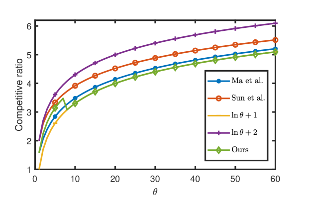
Figure 2. The competitive ratios obtained by Ma et al. (ma2020algorithms, ), Sun et al. (Sun2020Competitive, ) and ours. We fix $N=3$ and vary $\theta$ from $1$ to $60$.

6. Extension to General Concave Revenue Function

In addition to the set of revenue functions $\mathcal{G}$ we discuss above, our divide-and-conquer approach can be applied under a broader range of functions with corresponding applications. For example, we widely observe the logarithmic functions (e.g., $\log(v+1)$) in wireless communication (Niv2012Dynamic, ; Niv2010Multi, ), which is not covered by the revenue function set $\mathcal{G}$ when considering sufficiently large capacity. Also, the revenue functions in the application of one-way trading with price elasticity (cr_pursuit2018, ). In general, let us consider a given set of concave revenue functions with zero value at the origin; say $\tilde{\mathcal{G}}$. We define $\Phi_{\tilde{G}}(1)$ as the maximum online total allocation of running CR-Pursuit(1) under revenue functions $\tilde{\mathcal{G}}$ in the single inventory case (as defined in (17) with $\pi=1$). It represents the maximum capacity we required to maintain the same performance of the offline optimal at all time. We have the following results for the OOIC-M under the set of revenue functions $\tilde{\mathcal{G}}$.

Proposition 13.

Suppose we can find $\tilde{\pi}$ such that for OOIC-S, we have

(52) $$\Phi_{\tilde{G}}(1)\leq\tilde{\pi}\cdot C.$$

We can run the A&P($\tilde{\pi}$) for OOIC-M under $\tilde{\mathcal{G}}$. The competitive ratio of A&P($\tilde{\pi}$) is given by,

(53) $$\mathcal{CR}_{\tilde{G}}(\textsf{A\&P(${\tilde{\pi}}$)}=\begin{cases}\tilde{\pi},&\tilde{\pi}\geq N,\\ \frac{e^{\frac{1}{\tilde{\pi}}}}{e^{\frac{1}{\tilde{\pi}_{1}}}-1},&\tilde{\pi}<N.\end{cases}$$

The proof follow the same idea as discussed in Sec. 5 and is omitted here. When $\tilde{\pi}<N$, we simply recover Lemma 7 with the condition (52). Together with Theorem 9, we show the results in  (53) when $\tilde{\pi}\geq N$. As for the case $\tilde{\pi}<N$, we can recover Theorem 11 by noting that $\Phi_{\tilde{\mathcal{G}}}(\tilde{\pi})\leq\frac{1}{\tilde{\pi}}\Phi_{\tilde{\mathcal{G}}}(1)\leq C$ (due the concavity of the revenue functions), i.e., CR-Pursuit($\tilde{\pi}$) is feasible and $\tilde{\pi}$-competitive for OOIC-S.

For example, we can consider the one-way trading with price elasticity problem with multiple inventories, where the single-inventory case is proposed in (cr_pursuit2018, ). More specifically, we consider the following type of revenue function, which we denote as $\hat{\mathcal{G}}$.

• $g_{i,t}(v_{i,t})=\left(p_{i,t}-q_{i,t}(v_{i,t})\right)\cdot v_{i,t}$, $v_{i,t}\in[0,\delta_{i,t}]$, where $q_{i,t}(\cdot)$ is convex increasing function with $q_{i,t}(0)=0$ and $p_{i,t}\in[p_{\min},p_{\max}]$.

The revenue functions in $\hat{\mathcal{G}}$ consider that the price of selling (allocating) the inventory decreases as the supply (allocation) increases, which follows the basic law in supply and demand in microeconomics. In particular, the price elasticity is captured by a convex increasing function $q_{i,t}(\cdot)$, meaning that more supply would further decrease the price. The marginal revenue is bounded between $p_{\min}$ and $p_{\max}$ only at the origin and could be even zero otherwise, which implies $\hat{\mathcal{G}}$ is not covered by $\mathcal{G}$.

According to Lemma 15 in (cr_pursuit2018, ) (while it does not consider rate limit constraint, we can check that the proof simply follows with limit constraint), we have

(54) $$\Phi_{\hat{G}}(1)\leq 2\cdot(\ln\theta+1)\cdot C.$$

For OOIC-M under revenue function set, $\hat{\mathcal{G}}$, we have

Proposition 14.

Let $\pi_{2}=2\cdot(\ln\theta+1)$. A&P($\pi_{2}$) achieves the following competitive ratio for OOIC-M under revenue function set $\hat{\mathcal{G}}$,

(55) $$\mathcal{CR}_{\hat{\mathcal{G}}}(A\&P(\pi_{2}))=\begin{cases}\pi_{2},&\pi_{2}\geq N,\\ \frac{e^{\frac{1}{\pi_{2}}}}{e^{\frac{1}{\pi_{2}}}-1},&\pi_{2}<N.\end{cases}$$

The CR we achieve is upper bounded by $2\ln\theta+3$, which is up to a constant factor multiplying the lower bound $\ln\theta+1$. This provides the first CR of the OOIC-M under revenue function set $\hat{\mathcal{G}}$ with application to the one-way trading with price elasticity under multiple-inventory scenario. It is interesting to see whether we can fine a tiger bound on $\Phi_{\hat{\mathcal{G}}}(1)$ and achieve a better competitive ratio. In addition, while the determination of $\Phi_{\tilde{G}}(1)$ could be problem-specific, how we can show a general way for it would be another interesting future direction.

7. Concluding Remarks

In this work, we study the competitive online optimization problem under multiple inventories, OOIC-M. The online decision maker allocates the capacity-limited inventories to maximize the overall revenue, while the revenue functions and the allocation constraints at each slot come in an online manner. Our key result is a divide-and-conquer approach that reduces the multiple-inventory problem to the single-inventory case with a small optimality loss in terms of the CR. In particular, we show that our approach achieves the optimal when $N$ is small and is within an additive constant to the lower bound when $N$ is larger, when considering gradient bounded revenue functions. We also provide a general condition for applying our approach to broader applications with different interesting sets of revenue functions. In particular, for revenue functions appeared in one-way trading with price elasticity, our approach obtains an optimal CR for the problem that is up to a constant factor to the lower bound. As a by-product, we also provide the first allowance augmentation results for the online fractional matching problem and the online fraction allocation problem with free disposal. As a future direction, we are interested in how our divide-and-conquer approach can be used to solve other online optimization problems with multi-entity and how it can be applied in more application scenarios.

APPENDIX

Appendix A Proof of Proposition 1

Our proof follow the well-established online primal-and-dual approach [22, 13, 26, 28], etc.

We note that according to Appendix E of  [26]. The threshold function is increasing and satisfies the following conditions.

(56) $$C_{i}\phi_{i}^{\prime}(w)-\phi_{i}(w)\leq p_{\min}(\tilde{\chi}-1), \;w\in(0,\chi\cdot C_{i});$$

(57) $$C_{i}\phi_{i}^{\prime}(w)-\tilde{\chi}\cdot\phi_{i}(w)\leq 0, \;w\in(\chi\cdot C_{i},C_{i}).$$

Accordingly, it simply applies that

(58) $$C_{i}\phi_{i}(w)-\int_{0}^{w}\phi_{i}(w)dw\leq p_{\min}(\tilde{\chi}-1)\cdot w, \;w\in(0,\chi\cdot C_{i});$$

(59) $$C_{i}\phi_{i}(w)-\int_{0}^{w}\phi_{i}(w)\leq(\tilde{\chi}-1)\cdot\left(p_{min}\cdot\chi\cdot C_{i}+\int_{\chi\cdot C_{i}}^{w}\phi_{i}(w)dw\right), \;w\in(\chi\cdot C_{i},C_{i}).$$

In the primal-and-dual framework, it applies the dual problem as a baseline for the offline optimal. The dual problem of OOIC-M at slot $T$,

(60) $$\textsf{Dual-{OOIC-M}}:\;\quad \min\sum_{i,t\in[T]}h_{i,t}(\alpha_{i}+\beta_{t})+\sum_{i}{C_{i}\alpha_{i}}+\sum_{t}{A_{t}\beta_{t}}$$

(61) s.t. $$\alpha_{i}\geq 0,\beta_{t}\geq 0,\forall t,i,$$

where

(62) $$h_{i,t}(\lambda)=\max_{0\leq v\leq\delta_{i,t}}g_{i,t}(v)-\lambda\cdot v.$$

We denote the online solution of the algorithm as $\bar{v}_{i,t}$, which is the optimal solution to problem (P&D) in (8). Recall that $w_{i,t}$ is the online total allocation of the algorithm from slot $1$ to slot $t$, i.e.,

(63) $$w_{i,t}=\sum_{\tau=1}^{t}\bar{v}_{i,\tau}$$

At each slot $t$, we denote the optimal dual solution of problem (P&D) in (8) associated with constraint (9) as $\hat{\beta}_{t}$. Note that according to KKT conditional, we have

(64) $$\hat{\beta}_{t}\cdot(\sum_{i\in[N]}\bar{v}_{i,t}-A_{t})=0.$$

We consider the following dual solution,

(65) $$\alpha_{i}=\phi_{i}(w_{i,T}),\forall i;\beta_{t}=\hat{\beta}_{t},\forall t\in[T].$$

We note that the dual variable satisfies the dual constraint (61). Then, we have

(66) $$OPT_{T}\leq \sum_{i\in[N],t\in[T]}h_{i,t}(\alpha_{i}+\beta_{t})+\sum_{i\in[N]}C_{i}\alpha_{i}+\sum_{t\in[T]}A_{t}\beta_{t}$$

(67) $$= \sum_{i\in[N],t\in[T]}h_{i,t}(\phi_{i}(w_{i,T})+\hat{\beta}_{t})+\sum_{i\in[N]}C_{i}\phi_{i}(w_{i,T})+\sum_{t\in[T]}A_{t}\hat{\beta}_{t}$$

(68) $$\stackrel{{\scriptstyle(a)}}{{\leq}} \sum_{i\in[N],t\in[T]}h_{i,t}(\phi_{i}(w_{i,t})+\hat{\beta}_{t})+\sum_{i\in[N]}C_{i}\phi_{i}(w_{i,T})+\sum_{t\in[T]}A_{t}\hat{\beta}_{t}$$

(69) $$\stackrel{{\scriptstyle(b)}}{{\leq}} \sum_{i\in[N],t\in[T]}\left[g_{i,t}(\bar{v}_{i,t})-(\phi_{i}(w_{i,t})+\hat{\beta}_{t})\bar{v}_{i,t}\right]+\sum_{i\in[N]}C_{i}\phi_{i}(w_{i,T})+\sum_{t\in[T]}A_{t}\hat{\beta}_{t}$$

(70) $$\stackrel{{\scriptstyle(c)}}{{=}} \sum_{i\in[N],t\in[T]}\left[g_{i,t}(\bar{v}_{i,t})-\phi_{i}(w_{i,t})\bar{v}_{i,t}\right]+\sum_{i\in[N]}C_{i}\phi_{i}(w_{i,T})$$

(71) $$\stackrel{{\scriptstyle(d)}}{{\leq}} \sum_{i\in[N],t\in[T]}g_{i,t}(\bar{v}_{i,t})+\sum_{i\in[N]}\left[C_{i}\phi_{i}(w_{i,T})-\int_{0}^{w_{i,T}}\phi_{i}(w)dw\right]$$

(72) $$\stackrel{{\scriptstyle(e)}}{{\leq}} \tilde{\chi}\cdot\sum_{i\in[N],t\in[T]}g_{i,t}(\bar{v}_{i,t})$$

where (a) is due to the non-decreasing of $\phi_{i}(\cdot)$ and $h_{i,t}(\cdot)$ defined in (62); (b) is due to $\bar{v}_{i,t}$ is the optimal solution to (62) when $\lambda=\phi_{i}(w_{i,t})+\hat{\beta}_{t}$ by checking that the KKT conditions of the problem (P&D) in (8); (c) is according to (64); (d) is according to $\phi_{i}(w_{i,t})\bar{v}_{i,t}\geq\int_{w_{i,t}-\bar{v}_{i,t}}^{w_{i,t}}\phi_{i}(w)dw$; (e) is by the fact that

(73) $$C_{i}\phi_{i}(w_{i,T})-\int_{0}^{w_{i,T}}\phi_{i}(w)dw\leq(\tilde{\chi}-1)\sum_{t\in[T]}g_{i,t}(\bar{v}_{i,t}).$$

We show (73) in the following. When $w_{i,T}\leq\chi\cdot C_{i}$, it directly follows (58) and $\sum_{t\in[T]}g_{i,t}(\bar{v}_{i,t})\geq p_{min}\cdot w_{i,T}$. When $w_{i,T}\geq\chi\cdot C_{i}$, it follows  (59) and that

(74) $$\sum_{t\in[T]}g_{i,t}(\bar{v}_{i,t})\geq p_{\min}\cdot\chi\cdot C_{i}+\int_{\chi\cdot C_{i}}^{w_{i,T}}\phi_{i}(w)dw$$

by the fact that if $\bar{v}_{i,t}>0$,

(75) $$g^{\prime}_{i,t}(v)\geq max\{p_{\min},\phi_{i}(w_{i,{t-1}}+v)\},\forall v\leq\bar{v}_{i,t}$$

(75) is due to that $g^{\prime}_{i,t}(\bar{v}_{i,t})\geq max\{p_{\min},\phi_{i}(w_{i,t})\}$, which follows the concavity of $g_{i,t}(\cdot)$, non-decreasing property of $\phi_{i}(\cdot)$, and $g^{\prime}_{i,t}(\bar{v}_{i,t})\geq\phi_{i}(w_{i,t})$, if $\bar{v}_{i,t}>0$ by the KKT condition of (P&D) in (8).

Appendix B Proof of Lemma 4

We first consider a new class of revenue function,

• $g_{t}(v_{t})$ is concave, increasing and differentiable with $g_{t}(0)=0$;

• $\frac{g^{\prime}(0)}{g_{t}(\delta_{t})/\delta_{t}}\leq\xi$;

• $g^{\prime}_{t}(0)\in[p_{\min},p_{\max}]$

where $\xi$ is a given parameter. We denote this class of revenue function as Class_ξ. We can generalize the results (Theorem 8) in [21] by taking rate limit into consider and obtain the following proposition

Proposition 15.

For Class_ξ revenue function, we have

(76) $$\Phi_{\xi}(\pi)\leq\xi\cdot(\ln\theta+1)\cdot\frac{C}{\pi}$$

We omit the detailed proof here as it is by simply checking the proof in [21] step-by-step when considering revenue function $g_{t}(v_{t})$ defined over $v_{t}\in[0,\delta_{t}]$ instead of $v_{t}\in[0,C]$.

We now turn to the proof of Lemma 4.

Proof of Lemma 4.

We proof the lemma by showing that for any $\epsilon>0$, $\Phi_{1}(\pi)\leq(1+\epsilon)(\ln\theta+1)\cdot\frac{C}{\pi}$.

For any function $g_{t}(v_{t}),v_{t}\in[0,\delta_{t}]$, we can construct a sequence of functions as follows. We begin by finding the maximum $v^{(1)}\leq\delta_{t}$ such that $g^{\prime}_{t}(v^{(1)})\geq g_{t}^{\prime}(0)/(1+\epsilon)$. We define $g^{(1)}_{t}(v)=g_{t}(v),v\in[0,v^{(1)}]$. We then find the maximum $v^{(2)}\leq\delta_{t}$ such that $g^{\prime}_{t}(v^{(2)})\geq g_{t}^{\prime}(v^{(1)})/(1+\epsilon)$. We define $g^{(2)}_{t}(v)=g_{t}(v^{(1)}+v)-g_{t}(v^{(1)}),v\in[0,v^{(2)}-v^{(1)}]$. We continue the steps until we arrive at $\delta_{t}$. Suppose in total there are $k_{t}$ functions we construct, and they are $\{g^{(i)}(v)\}_{i\in k_{t}}$, where $g^{(i)}(v)=g_{t}(v^{(i-1)}+v)-g_{t}(v^{(i-1)}),v\in[0,v^{(i)}-v^{(i-1)}]$. Also, $v^{(k)}=\delta_{t}$. We can easily check that $\{g^{(i)}(v)\}_{i\in k_{t}}$ belongs to Class_ξ=1+ϵ.

For any $\sigma\in\Sigma$, suppose there is a revenue function $g_{t}(v_{t})$ not belonging to Class_ξ=1+ϵ, we can construct $\{g^{(i)}(v)\}_{i\in k_{t}}$ following the above procedure and replace $g_{t}(v_{t})$ in $\sigma$. We denote the new input as $\tilde{\sigma}$. We can show that the replacement will not decreasing the total allocation of CR-Pursuit($\pi$), We note that the output of CR-Pursuit($\pi$) does not change at $\tau\neq t$ as the venue function and increment of the optimal objective remains the same at those slots. Thus it is sufficient to show that

(77) $$\hat{v}_{t}\leq\sum_{i=1}^{k_{t}}{\tilde{v}_{t}^{(i)}}$$

, where $\hat{v}_{t}$ is the output of CR-Pursuit($\pi$)  under $\sigma$ at slot $t$ and $\tilde{v}_{t}^{(i)}$ is the output of CR-Pursuit($\pi$)  under $\tilde{\sigma}$ at function $g_{t}^{(i)}(\cdot)$, for $i\in[k_{t}]$. Following the CR-Pursuit($\pi$) algorithm, we have

(78) $$g_{t}(\hat{v}_{t})=\frac{1}{\pi}(OPT(t)-OPT(t-1))=\sum_{i=1}^{k_{t}}g_{t}^{(i)}({\tilde{v}_{t}^{(i)}})$$

According to our construction and concavity of $g_{t}(\cdot)$, we have

(79) $$\sum_{i=1}^{k_{t}}g_{t}^{(i)}({\tilde{v}_{t}^{(i)}}) =\sum_{i=1}^{k_{t}}\left[g_{t}(v^{(i-1)}+{\tilde{v}_{t}^{(i)}})-g_{t}(v^{(i-1)})\right]$$

(80) $$\stackrel{{\scriptstyle(a)}}{{\leq}}\sum_{i=1}^{k_{t}}\left[g_{t}(\sum_{j=1}^{i-1}{\tilde{v}_{t}^{(j)}}+{\tilde{v}_{t}^{(i)}})-g_{t}(\sum_{j=1}^{i-1}{\tilde{v}_{t}^{(j)}})\right]$$

(81) $$=g_{t}(\sum_{i=1}^{k_{t}}{\tilde{v}_{t}^{(i)}})$$

, where (a) is due to the concavity of $g_{t}(\cdot)$ and the fact that $\sum_{j=1}^{i-1}{\tilde{v}_{t}^{(j)}}\leq\sum_{j=1}^{i-1}{({v}^{(j)}-{v}^{(j-1)})}\leq v^{(i-1)},\forall i\in[t_{k}]$. Thus, we have $g_{t}(\hat{v}_{t})\leq g_{t}(\sum_{i=1}^{k_{t}}{\tilde{v}_{t}^{(i)}})$ and conclude (77).

This directly implies that we can replace all functions by a sequence of Class_ξ=1+ϵ functions without decreasing the total allocation of CR-Pursuit($\pi$). Thus, $\Phi(\pi)\leq\Phi_{\xi=1+\epsilon}(\pi)\leq(1+\epsilon)\cdot(\ln\theta+1)\cdot\frac{C}{\pi},\forall\epsilon>0$. And, we conclude $\Phi(\pi)\leq(\ln\theta+1)\cdot\frac{C}{\pi}$

∎

Appendix C Proof of Theorem 9

We first show a useful proposition.

Proposition 16.

$\Psi_{i,t}(a)$ is non-decreasing in $a$.

Proof.

By integration by parts,

(82) $$\int_{0}^{c_{i}}f_{i}(x)\frac{\partial G_{i,t}(x,a)}{\partial x}dx= \int_{0}^{c_{i}}f_{i}(x)dG_{i,t}\left(x,a\right)$$

(83) $$= \left.f_{i}(x)\cdot G_{i,t}\left(x,a\right)\right|_{0}^{C_{i}}-\frac{1}{\pi\cdot C_{i}}\int_{0}^{C_{i}}f_{i}(x)G_{i,t}\left(x,a\right)dx$$

(84) $$= f_{i}(C_{i})G_{i,t}\left(C_{i},a\right)-\frac{1}{\pi\cdot C_{i}}\int_{0}^{C_{i}}f_{i}(x)G_{i,t}\left(x,a\right)dx$$

(85) $$= \Psi_{i,t}(a)$$

And according to the sensitivity analysis of the optimization problem defining $G_{i,t}(x,a)$, we have

(86) $$\frac{\partial G_{i,t}(x,a)}{\partial x}=\eta^{*}.$$

where $\eta^{*}$ is the optimal dual variable associated with constraint (41). We can check that $\eta^{*}$ is non-decreasing in $a$ by the KKT condition, and thus $\Psi_{i,t}(a)$ is non-decreasing in $a$. ∎

Proof of Theorem 9.

We adapt the primal-and-dual framework [13, 19] to prove the theorem. We begin with the revenue increment of our algorithm AAt($\pi$)-A at slot $t$, denoted as $\Delta P$. According to  (40),

(87) $$\Delta P\triangleq\sum_{i}\left(\tilde{OPT}_{i,t}-\tilde{OPT}_{i,t-1}\right)=\sum_{i}\left(G_{i,t}(C_{i},\hat{a}_{i,t})-G_{i,t}(C_{i},0)\right).$$

We note that the optimal solution of AAt($\pi$)-A satisfies the KKT condition,

(88) $$\tilde{g}^{\prime}_{i,t}(\hat{a}_{i,t})-\Psi_{i,t}(\hat{a}_{i,t})-\tilde{\beta}_{t}-\tilde{\gamma}_{i,t}+\tilde{\sigma}_{i,t}=0,\forall i$$

(89) $$\tilde{\beta}_{t}\left(\sum_{i}\hat{a}_{i,t}-\pi\cdot A_{t}\right)=0,$$

(90) $$\tilde{\sigma}_{i,t}\cdot\hat{a}_{i,t}=0,\forall i,$$

(91) $$\tilde{\gamma}_{i,t}\left(\hat{a}_{i,t}-\pi\cdot\delta_{i,t}\right)=0,\forall i,$$

, where $\tilde{\beta}_{t}\geq 0$ and $\tilde{\sigma}_{t}^{i}\geq 0,\tilde{\gamma}_{t}^{i}\geq 0,\forall i$ are dual variables corresponding to constraints (36) and (LABEL:eq:AAt-rate)).

We first write down the dual problem of OOIC-M at slot $t$,

(92) $$\textsf{Dual-{OOIC-M}}:\;\quad \min\sum_{i,\tau\in[t]}h_{i,\tau}(\alpha_{i}+\beta_{\tau})+\sum_{i}{C_{i}\alpha_{i}}+\sum_{\tau}{A_{\tau}\beta_{\tau}}$$

(93) s.t. $$\alpha_{i}\geq 0,\beta_{t}\geq 0,\forall t,i,$$

where

(94) $$h_{i,\tau}(\lambda)=\max_{0\leq v\leq\delta_{i,\tau}}g_{i,\tau}(v)-\lambda\cdot v.$$

We compare our online increment with the following dual solution. At slot $t$, we update the dual variable $\{\alpha_{i,t}\}_{i\in[N]}$, determine the dual variable $\beta_{t}$,

(95) $$\alpha_{i,t}=\Psi_{i,t}(\hat{a}_{i,t}),\forall i;\beta_{t}=\tilde{\beta}_{t}.$$

We note that the dual variable satisfies the dual constraint (93).

Let the increment of the dual objective by above dual solutions at each slot as $\Delta D$. To proof the theorem, the most important step in the framework is to show that at each slot, we have

(96) $$\Delta D\leq\frac{1}{\pi}\frac{e^{\frac{1}{\pi}}}{e^{\frac{1}{\pi}}-1}{\Delta P}$$

We can now compute the increment of the dual,

$$\Delta D =\sum_{i,\tau<t}\left(h_{i,\tau}\left(\alpha_{i,t}+{\beta}_{\tau}\right)-h_{i,\tau}\left(\alpha_{i,t-1}+{\beta}_{\tau}\right)\right)$$

(97) $$\quad+\sum_{i}h_{i,t}\left(\alpha_{i,t}+{\beta}_{t}\right)+\sum_{i}C_{i}\left(\alpha_{i,t}-\alpha_{i,t-1}\right)+\beta_{t}A_{t}$$

(98) $$\stackrel{{\scriptstyle(a)}}{{\leq}}\sum_{i}h_{i,t}\left(\Psi_{i,t}(\hat{a}_{i,t})+\tilde{\beta}_{t}\right)+\sum_{i}C_{i}\left(\Psi_{i,t}(\hat{v}_{i,t})-\Psi_{i,t}(0)\right)+\tilde{\beta}_{t}A_{t}$$

(99) $$\stackrel{{\scriptstyle(b)}}{{=}}\sum_{i}\frac{1}{\pi}\left[\tilde{g}_{i,t}(\hat{a}_{i,t})-\left(\Psi_{i,t}(\hat{a}_{i,t})+\tilde{\beta}_{t}\right)\hat{a}_{i,t}\right]+\sum_{i}C_{i}\left(\Psi_{i,t}(\hat{a}_{i,t})-\Psi_{i,t}(0)\right)+\tilde{\beta}_{t}A_{t}$$

(100) $$\stackrel{{\scriptstyle(c)}}{{=}}\sum_{i}C_{i}\left(\Psi_{i,t}\left(\hat{a}_{i,t}\right)-\Psi_{i,t}(0)\right)+\frac{1}{\pi}\sum_{i}\left(\tilde{g}_{i,t}(\hat{a}_{i,t})-\Psi_{i,t}(\hat{a}_{i,t})\cdot\hat{a}_{i,t}\right)$$

We show the above equality of inequality one-by-one.

• (a) is according to (95) (the way to set the dual variables) and the facts that $a_{i,t}\geq a_{i,t-1}$ and $h_{i,t}(\lambda)$ is non-increasing in $\lambda$.

• (b) is according to the fact that by (88), (90) and (91)$,\hat{a}_{i,t}$ is the optimal solution to

  (101) $$\max_{0\leq v\leq\pi\cdot\delta_{i,\tau}}\tilde{g}_{i,\tau}(v)-\left(\Psi_{i,t}(\hat{a}_{i,t})+\tilde{\beta}_{t}\right)\cdot v.$$

  Also, we have

  (102) $$\max_{0\leq v\leq\pi\cdot\delta_{i,\tau}}\tilde{g}_{i,\tau}(v)-\left(\Psi_{i,t}(\hat{a}_{i,t})+\tilde{\beta}_{t}\right)\cdot v$$

  (103) $$= \max_{0\leq v\leq\pi\cdot\delta_{i,\tau}}\pi\cdot g_{i,\tau}(\frac{v}{\pi})-\left(\Psi_{i,t}(\hat{a}_{i,t})+\tilde{\beta}_{t}\right)\cdot v$$

  (104) $$= \pi\cdot\max_{0\leq v\leq\pi\cdot\delta_{i,\tau}}\pi\cdot g_{i,\tau}(\frac{v}{\pi})-\left(\Psi_{i,t}(\hat{a}_{i,t})+\tilde{\beta}_{t}\right)\cdot\frac{v}{\pi}$$

  (105) $$= \pi\cdot\max_{0\leq v\leq\delta_{i,\tau}}\pi\cdot g_{i,\tau}(v)-\left(\Psi_{i,t}(\hat{a}_{i,t})+\tilde{\beta}_{t}\right)\cdot v$$

  (106) $$= \pi\cdot h_{i,t}\left(\Psi_{i,t}(\hat{a}_{i,t})+\tilde{\beta}_{t}\right).$$

• (c) is according to (89).

Recall (38) that

$$\Psi_{i,t}(a)=f_{i}(C_{i})\cdot G_{i,t}(C_{i},a)-\frac{1}{\pi\cdot C_{i}}\int_{0}^{C_{i}}G_{i,t}\left(x,a\right)\cdot f_{i}(x)dx.$$

Plugging $\Psi_{i,t}(\cdot)$, i.e., (38)), in $\Delta D$, we have that

(107) $$\Delta D =\sum_{i}\left\{C_{i}\cdot f_{i}(C_{i})G_{i,t}\left(C_{i},\hat{a}_{i,t}\right)-\frac{1}{\pi}\cdot\int_{0}^{C_{i}}f_{i}(x)G_{i,t}\left(x,\hat{a}_{i,t}\right)dx\right.$$

(108) $$\left.-\left(f_{i}(C_{i})G_{i,t}\left(C_{i},0\right)-\frac{1}{\pi}\cdot\int_{0}^{C_{i}}f_{i}(x)G_{i,t}\left(x,0\right)dx\right)+\frac{1}{\pi}\cdot\left(\tilde{g}_{i,t}(\hat{a}_{i,t})-\Psi_{i,t}(\hat{a}_{i,t})\cdot\hat{a}_{i,t}\right)\right\}$$

By the fact that $C_{i}\cdot f_{i}(C_{i})=\frac{1}{\pi}\frac{e^{\frac{1}{\pi}}}{e^{\frac{1}{\pi}}-1}$ according to  (39), we have

$$\Delta D= \frac{1}{\pi}\frac{e^{\frac{1}{\pi}}}{e^{\frac{1}{\pi}}-1}\sum_{i}\left[G_{i,t}\left(C_{i},\hat{a}_{i,t}\right)-G_{i,t}\left(C_{i},0\right)\right]$$

$$+\sum_{i}\left[-\frac{1}{\pi}\cdot\int_{0}^{C_{i}}f_{i}(x)G_{i,t}\left(x,\hat{a}_{i,t}\right)dx+\frac{1}{\pi}\cdot\int_{0}^{C_{i}}f_{i}(x)G_{i,t}\left(x,0\right)dx\right]$$

(109) $$+\sum_{i}\frac{1}{\pi}\cdot\left(\tilde{g}_{i,t}(\hat{a}_{i,t})-\Psi_{i,t}(\hat{a}_{i,t})\cdot\hat{a}_{i,t}\right)$$

Comparing with (87), to show (96), is sufficient to show that

(110) $$\tilde{g}_{i,t}(\hat{a}_{i,t})-\Psi_{i,t}(\hat{a}_{i,t})\cdot\hat{a}_{i,t}\leq\int_{0}^{C_{i}}f_{i}(x)G_{i,t}\left(x,\hat{a}_{i,t}\right)dx-\int_{0}^{C_{i}}f_{i}(x)G_{i,t}\left(x,0\right)dx$$

We further have

(111) $$\tilde{g}_{i,t}(\hat{a}_{i,t})-\Psi_{i,t}(\hat{a}_{i,t})\cdot\hat{a}_{i,t}$$

(112) $$\leq\tilde{g}_{i,t}(\hat{a}_{i,t})-\int_{0}^{\hat{a}_{i,t}}\Psi_{i,t}(a)da$$

(113) $$\leq\tilde{g}_{i,t}(\hat{a}_{i,t})-\int_{0}^{\hat{a}_{i,t}}\left[f_{i}(C_{i})\cdot G_{i,t}(C_{i},a)-\frac{1}{C_{i}}\int_{0}^{C_{i}}G_{i,t}\left(x,a\right)\cdot f_{i}(x)dx\right]da$$

(114) $$\stackrel{{\scriptstyle(a)}}{{=}}\tilde{g}_{i,t}(\hat{a}_{i,t})-\int_{0}^{\hat{a}_{i,t}}\int_{0}^{c_{i}}\frac{\partial G_{i,t}(x,a)}{\partial x}\cdot f_{i}(x)dxda$$

(115) $$=\int_{0}^{c_{i}}\int_{0}^{\hat{a}_{i,t}}\tilde{g}^{\prime}_{i,t}(a)-\frac{\partial G_{i,t}(x,a)}{\partial x}da\cdot f_{i}(x)dx$$

, where (a) is due to  (85).

So, it reduces to show that

(116) $$\int_{0}^{\hat{a}_{i,t}}\tilde{g}^{\prime}_{i,t}(a)-\frac{\partial G_{i,t}(x,a)}{\partial x}da\leq G_{i,t}\left(x,\hat{a}_{i,t}\right)-G_{i,t}\left(x,0\right)$$

, which is equivalent to

(117) $$\int_{0}^{\hat{a}_{i,t}}\tilde{g}^{\prime}_{i,t}(a)-\frac{\partial G_{i,t}(x,a)}{\partial x}da\leq\int_{0}^{\hat{a}_{i,t}}\frac{\partial G_{i,t}(x,a)}{\partial a}da.$$

To show the above inequality, it is sufficient to show that,

(118) $$\tilde{g}^{\prime}_{i,t}(a)\leq\frac{\partial G_{i,t}(x,a)}{\partial x}+\frac{\partial G_{i,t}(x,a)}{\partial a}.$$

To proceed, we recall that $G_{i,t}(x,a)$ is the optimal objective to the following problem,

(119) $$G_{i,t}\left(x,a\right)=\max\quad \sum_{\tau\in[t]}\tilde{g}_{i,\tau}(v_{i,\tau})$$

(120) s.t $$\sum_{\tau\in[t]}v_{i,\tau}\leq x$$

(121) $$0\leq v_{i,t}\leq a$$

(122) $$0\leq v_{i,\tau}\leq\hat{a}_{i,\tau},\forall\tau\in[t-1].$$

Let $\eta$, $\psi_{t}$ and $\phi_{t}$, and $\{\psi_{\tau}\}_{\tau\in[t-1]}$ and $\{\phi_{\tau}\}_{\tau\in[t-1]}$ be the dual variable associated with (120), (121), and (122), respectively.

According to sensitivity analysis of convex program, we have

(123) $$\frac{\partial G_{i,t}(x,a)}{\partial x}=\eta^{*},\frac{\partial G_{i,t}(x,a)}{\partial a}=\phi_{t}^{*}$$

According to the KKT condition of the optimal solution, we have

(124) $$\tilde{g}^{\prime}_{i,t}(a)\leq\tilde{g}^{\prime}_{i,t}(v_{i,t}^{*})=\eta^{*}+\phi_{t}^{*}-\psi_{t}^{*}\leq\eta^{*}+\phi_{t}^{*}$$

, where $v_{i,t}^{*}$, $\phi_{t}^{*}$, $\psi_{t}^{*}$, $\eta^{*}$ and $\phi_{t}^{*}$ represent the optimal primal solution and dual solution, and the first inequality is due to the fact that $\tilde{g}_{i,t}(\cdot)$ is concave and $v_{i,t}^{*}\leq a$.

Combining (123) and (124), we conclude (118), which leads to (116) and (117). Combining (115) and (116), we conclude (110). Combining  (110), (87) and  (109), we easily conclude (96). Summing (96) over all time slot, we have

(125) $$\sum_{i\in[N]}\tilde{OPT}_{i,t}\geq\pi\cdot\frac{e^{\frac{1}{\pi}}-1}{e^{\frac{1}{\pi}}}\cdot\text{Dual-OOIC-M}\geq\pi\cdot\frac{e^{\frac{1}{\pi}}-1}{e^{\frac{1}{\pi}}}\cdot OPT_{t}$$

∎

References

- [1] Shizhen Zhao, Xiaojun Lin, and Minghua Chen. Robust online algorithms for peak-minimizing ev charging under multistage uncertainty. IEEE Transactions on Automatic Control, 62(11):5739–5754, 2017.
- [2] Bahram Alinia, Mohammad Sadegh Talebi, Mohammad H Hajiesmaili, Ali Yekkehkhany, and Noel Crespi. Competitive online scheduling algorithms with applications in deadline-constrained ev charging. In 2018 IEEE/ACM 26th International Symposium on Quality of Service (IWQoS), pages 1–10. IEEE, 2018.
- [3] Qiulin Lin, Hanling Yi, and Minghua Chen. Minimizing cost-plus-dissatisfaction in online ev charging under real-time pricing. IEEE Transactions on Intelligent Transportation Systems, 2021.
- [4] Shuoyao Wang, Suzhi Bi, Ying-Jun Angela Zhang, and Jianwei Huang. Electrical vehicle charging station profit maximization: Admission, pricing, and online scheduling. IEEE Transactions on Sustainable Energy, 9(4):1722–1731, 2018.
- [5] Lian Lu, Jinlong Tu, Chi-Kin Chau, Minghua Chen, and Xiaojun Lin. Online energy generation scheduling for microgrids with intermittent energy sources and co-generation. ACM SIGMETRICS Performance Evaluation Review, 41(1):53–66, 2013.
- [6] Ying Zhang, Mohammad H Hajiesmaili, Sinan Cai, Minghua Chen, and Qi Zhu. Peak-aware online economic dispatching for microgrids. IEEE transactions on smart grid, 9(1):323–335, 2016.
- [7] Yanfang Mo, Qiulin Lin, Minghua Chen, and S. Joe Qin. Optimal online algorithms for peak-demand reduction maximization with energy storage. In Proc. ACM e-Energy, pages 73–83, 2021.
- [8] Yanfang Mo, Qiulin Lin, Minghua Chen, and S. Joe Qin. Optimal peak-minimizing online algorithms for large-load users with energy storage. In IEEE INFOCOM, 2021. poster paper.
- [9] Minghong Lin, Adam Wierman, Lachlan LH Andrew, and Eno Thereska. Dynamic right-sizing for power-proportional data centers. IEEE/ACM Transactions on Networking, 21(5):1378–1391, 2012.
- [10] Tan Lu, Minghua Chen, and Lachlan LH Andrew. Simple and effective dynamic provisioning for power-proportional data centers. IEEE Transactions on Parallel and Distributed Systems, 24(6):1161–1171, 2012.
- [11] Ming Shi, Xiaojun Lin, Sonia Fahmy, and Dong-Hoon Shin. Competitive online convex optimization with switching costs and ramp constraints. In IEEE INFOCOM 2018-IEEE Conference on Computer Communications, pages 1835–1843. IEEE, 2018.
- [12] Linqi Guo, John Pang, and Anwar Walid. Joint placement and routing of network function chains in data centers. In IEEE INFOCOM 2018-IEEE Conference on Computer Communications, pages 612–620. IEEE, 2018.
- [13] Niv Buchbinder and Joseph Naor. The design of competitive online algorithms via a primal-dual approach. Now Publishers Inc, 2009.
- [14] Aranyak Mehta. Online matching and ad allocation. Foundations and Trends in Theoretical Computer Science, 8(4):265–368, 2013.
- [15] Yunhong Zhou, Deeparnab Chakrabarty, and Rajan Lukose. Budget constrained bidding in keyword auctions and online knapsack problems. In International Workshop on Internet and Network Economics, pages 566–576. Springer, 2008.
- [16] Ran El-Yaniv, Amos Fiat, Richard M Karp, and Gordon Turpin. Optimal search and one-way trading online algorithms. Algorithmica, 30(1):101–139, 2001.
- [17] Minghong Lin, Adam Wierman, Alan Roytman, Adam Meyerson, and Lachlan LH Andrew. Online optimization with switching cost. ACM SIGMETRICS Performance Evaluation Review, 40(3):98–100, 2012.
- [18] Nikhil Bansal, Anupam Gupta, Ravishankar Krishnaswamy, Kirk Pruhs, Kevin Schewior, and Cliff Stein. A 2-competitive algorithm for online convex optimization with switching costs. In Approximation, Randomization, and Combinatorial Optimization. Algorithms and Techniques (APPROX/RANDOM 2015). Schloss Dagstuhl-Leibniz-Zentrum fuer Informatik, 2015.
- [19] Jon Feldman, Nitish Korula, Vahab Mirrokni, S. Muthukrishnan, and Martin Pál. Online ad assignment with free disposal. In Stefano Leonardi, editor, Internet and Network Economics, pages 374–385, Berlin, Heidelberg, 2009. Springer Berlin Heidelberg.
- [20] Nikhil R. Devanur and Kamal Jain. Online matching with concave returns. In Proceedings of the Forty-Fourth Annual ACM Symposium on Theory of Computing, STOC ’12, page 137–144, New York, NY, USA, 2012. Association for Computing Machinery.
- [21] Qiulin Lin, Hanling Yi, John Pang, Minghua Chen, Adam Wierman, Michael Honig, and Yuanzhang Xiao. Competitive online optimization under inventory constraints. Proc. ACM Meas. Anal. Comput. Syst., 3(1), March 2019.
- [22] Bo Sun, Ali Zeynali, Tongxin Li, Mohammad Hajiesmaili, Adam Wierman, and Danny H.K. Tsang. Competitive algorithms for the online multiple knapsack problem with application to electric vehicle charging. Proc. ACM Meas. Anal. Comput. Syst., 4(3), December 2020.
- [23] Yossi Azar and Arik Litichevskey. Maximizing throughput in multi-queue switches. Algorithmica, 45(1):69–90, 2006.
- [24] Bala Kalyanasundaram and Kirk R. Pruhs. An optimal deterministic algorithm for online b-matching. Theoretical Computer Science, 233(1):319–325, 2000.
- [25] Han Deng and I-Hong Hou. Optimal capacity provisioning for online job allocation with hard allocation ratio requirement. IEEE/ACM Transactions on Networking, 26(2):724–736, 2018.
- [26] Will Ma and David Simchi-Levi. Algorithms for online matching, assortment, and pricing with tight weight-dependent competitive ratios. Operations Research, 68(6):1787–1803, 2020. Available on arXiv in May 2019, https://arxiv.org/abs/1905.04770.
- [27] Nikhil R. Devanur, Kamal Jain, and Robert D. Kleinberg. Randomized primal-dual analysis of ranking for online bipartite matching. SODA ’13, page 101–107, USA, 2013. Society for Industrial and Applied Mathematics.
- [28] Rad Niazadeh and Robert D. Kleinberg. A unified approach to online allocation algorithms via randomized dual fitting. CoRR, abs/1308.5444, 2013.
- [29] Julian Lorenz, Konstantinos Panagiotou, and Angelika Steger. Optimal algorithms for k-search with application in option pricing. Algorithmica, 55(2):311–328, 2009.
- [30] Richard M Karp, Umesh V Vazirani, and Vijay V Vazirani. An optimal algorithm for on-line bipartite matching. In Proceedings of the twenty-second annual ACM symposium on Theory of computing, pages 352–358, 1990.
- [31] Yossi Azar, Niv Buchbinder, TH Hubert Chan, Shahar Chen, Ilan Reuven Cohen, Anupam Gupta, Zhiyi Huang, Ning Kang, Viswanath Nagarajan, Joseph Naor, et al. Online algorithms for covering and packing problems with convex objectives. In 2016 IEEE 57th Annual Symposium on Foundations of Computer Science (FOCS), pages 148–157. IEEE, 2016.
- [32] Han Deng, Tao Zhao, and I-Hong Hou. Online routing and scheduling with capacity redundancy for timely delivery guarantees in multihop networks. IEEE/ACM Transactions on Networking, 27(3):1258–1271, 2019.
- [33] Niv Buchbinder, Liane Lewin-Eytan, Ishai Menache, Joseph Naor, and Ariel Orda. Dynamic power allocation under arbitrary varying channels—an online approach. IEEE/ACM Transactions on Networking, 20(2):477–487, 2012.
- [34] Niv Buchbinder, Liane Lewin-Eytan, Ishai Menache, Joseph Naor, and Ariel Orda. Dynamic power allocation under arbitrary varying channels - the multi-user case. In 2010 Proceedings IEEE INFOCOM, pages 1–9, 2010.