On the Stability of Super-Resolution and
a Beurling–Selberg Type Extremal Problem

Abstract

Super-resolution estimation is the problem of recovering a stream of spikes (point sources) from the noisy observation of a few numbers of its first trigonometric moments. The performance of super-resolution is recognized to be intimately related to the separation between the spikes to recover. A novel notion of stability of the Fisher information matrix (FIM) of the super-resolution problem is introduced when the minimal eigenvalue of the FIM is not asymptotically vanishing. The regime where the minimal separation is inversely proportional to the number of acquired moments is considered. It is shown that there is a separation threshold above which the eigenvalues of the FIM can be bounded by a quantity that does not depend on the number of moments. The proof relies on characterizing the connection between the stability of the FIM and a generalization of the Beurling–Selberg box approximation problem.

I Introduction

The classical formulation of super-resolution consists of recovering a stream of point sources (or spikes), characterized by their amplitudes and positions from noisy and distorted measurements. This popular setup serves as a parametric model for many inverse problems in applied and experimental sciences, such as spectrum analysis, system identification, radar, sonar, and optical imaging [1, 2], as well as wireless communications and sensing systems. When the distortion is modeled by a low-pass, bandlimited, shift-invariant point spread function (PSF), the super-resolution problem is also referred to as line spectral estimation, considered herein.

While super-resolution has been persistently studied from both theoretical and algorithmic perspectives for several decades, many open related statistical challenges remain. In particular, a complete stability analysis in the presence of noise has not occurred. Herein, the study of the stability of the Fisher information matrix (FIM) of the super-resolution problem, which is defined by the non-vanishing asymptotic of its smallest eigenvalue when the problem dimension becomes large, is undertaken. The existence of a minimal separation between the sources above which the FIM is stable is established. Through the Cramér–Rao lower bound (CRLB), a new algorithm-free statistical resolution limit to stably recover the point sources is provided. The proof relies on relating the extremal singular values of some generalized Vandermonde matrices, with a novel extension of the Beurling–Selberg box approximation problem.

I-A Contributions and Organization of the Paper

Section II describes the signal model and defines the super-resolution model that would be considered in this work. After a review of the existing statistical and algorithmic resolution bounds, the notion of stability of the FIM is presented in Definition 1 and connected to the CRLB. The main result of this work is that the stability of the FIM for super-resolution is guaranteed whenever the separation parameter of the problem is greater than $3.54$. This result is presented in Proposition 3. The key technical result relies on the bounding of the extremal singular values of the sensitivity matrix of the problem. Further, relevant bounds are established in Lemma 4 as a function of the separation between the point sources.

The remainder of the paper provides the proof of Lemma 4. In Section III, a connection between the Beurling–Selberg box approximation problem and the condition number of Vandermonde matrices with nodes on the unit circle is recalled from the literature. Based on this observation, a novel box approximation problem by bandlimited functions is defined, and a relationship between the solution of this problem and the conditioning of the sensitivity matrix is given in Proposition 6. A pair of sub-optimal solutions to the box approximation problem is constructed whenever the separation parameter is large enough, yielding the numerical bounds of Proposition 3. A detailed proof of Proposition 6 is given in Section IV. Conclusions and future works are drawn in Section V.

I-B Notation and Definitions

Vectors of ${\mathbb{C}}^{N}$ and matrices of $\mathbb{C}^{N\times r}$ are denoted by boldface letters $\bm{a}$ and capital boldface letters $\bm{A}$, respectively. The minimal (resp. maximal) eigenvalues and singular values of a matrix $\bm{A}$ are denoted $\lambda_{\min}(\bm{A})$, $\sigma_{\min}(\bm{A})$ (resp. $\lambda_{\max}(\bm{A})$, $\sigma_{\max}(\bm{A})$). For any function $g\in L_{1}(\mathbb{R})$, we denote by $\widehat{g}$ its continuous time Fourier transform, defined as

$$\widehat{g}(u)=\int_{\mathbb{R}}g(t)e^{-i2\pi ut}dt,\quad\forall u\in\mathbb{R}.$$ (1)

A function $g\in L_{1}(\mathbb{R})$ is said to be $\beta$-bandlimited if for all $u$ such that $\left|u\right|>\beta$, we have $\widehat{g}(u)=0$. For any $\alpha>0$, $I_{\alpha}$ is the indicator function of the interval $[-\alpha/2,\alpha/2]$, i.e.,

$$I_{\alpha}(t)=\begin{cases}1&\mbox{if }\left|t\right|\leq\alpha/2,\\ 0&\mbox{otherwise.}\end{cases}$$ (2)

which we call the box function. We let $\mathbb{T}=\mathbb{R}/\mathbb{Z}$ to be the unidimensional torus. Let $N=2n+1$ be an odd number, then for any $\tau\in\mathbb{T}$, we denote by $\bm{v}_{0}(\tau)\in\mathbb{C}^{N}$ and $\bm{v}_{1}(\tau)=\frac{\mathrm{d}\bm{v}_{0}(\tau)}{\mathrm{d}\tau}/{\left\lVert\frac{\mathrm{d}\bm{v}_{0}(\tau)}{\mathrm{d}\tau}\right\rVert_{2}}\in\mathbb{C}^{N}$ the unit norm vectors

$$\bm{v}_{0}(\tau)={} \frac{1}{\sqrt{N}}\left[e^{-i2\pi(-n)\tau},\dots,e^{-i2\pi n\tau}\right]^{\top}$$ (3a)

$$\bm{v}_{1}(\tau)={} \frac{C_{N}}{\sqrt{N}}\left[-i2\pi(-n)e^{-i2\pi(-n)\tau},\dots,-i2\pi ne^{-i2\pi n\tau}\right]^{\top},$$ (3b)

where $C_{N}=\sqrt{\frac{3}{\pi^{2}(N-1)(N+1)}}$ is a normalization constant. For any vector $\bm{\tau}={[\tau_{1},\dots,\tau_{r}]}^{{\mathsf{T}}}\in{\mathbb{T}}^{r}$, we define by $\bm{V}_{0}(\bm{\tau}),\bm{V}_{1}(\bm{\tau})\in\mathbb{C}^{N\times r}$, the generalized Vandermonde matrices

$$\bm{V}_{0}(\bm{\tau})={} \left[\bm{v}_{0}(\tau_{1}),\dots,\bm{v}_{0}(\tau_{r})\right],$$ (4a)

$$\bm{V}_{1}(\bm{\tau})={} \left[\bm{v}_{1}(\tau_{1}),\dots,\bm{v}_{1}(\tau_{r})\right].$$ (4b)

The concatenation $\bm{W}(\bm{\tau})=[\bm{V}_{0}(\bm{\tau}),\bm{V}_{1}(\bm{\tau})]\in\mathbb{C}^{N\times 2r}$ is refereed to as the sensitivity matrix. Finally, the wrap-around distance $\Delta(\bm{\tau})$ is defined by the minimal distance between two pairs of points in $\bm{\tau}$ over the torus, i.e. $\Delta(\bm{\tau})\triangleq\min_{\ell\neq\ell^{\prime}}\inf_{j\in\mathbb{Z}}\left|\tau_{\ell}-\tau_{\ell^{\prime}}+j\right|$.

II The Stability of Super-Resolution

II-A Signal Model

Consider $r$ sources characterized by a vector $\bm{c}={[c_{1},\dots,c_{r}]}^{{\mathsf{T}}}\in\mathbb{C}^{r}$ of $r$ complex amplitudes, and a vector $\bm{\tau}={[\tau_{1},\dots,\tau_{r}]}^{{\mathsf{T}}}\in\mathbb{T}^{r}$. Our super-resolution problem is to estimate the $2r$ parameters $\{\bm{c},\bm{\tau}\}$ of the continuous time domain signal $x(t)=\sum_{\ell=1}^{r}c_{\ell}\delta(t-\tau_{\ell})$ from the noisy observation $\bm{y}=[y_{-n},\dots,y_{0},\dots y_{n}]\in\mathbb{C}^{N}$ of the form

$$\bm{y}={} {\left[\widehat{x}(-n),\dots,\widehat{x}(n)\right]}^{{\mathsf{T}}}+\bm{w}$$

$$={} \sum_{\ell=1}^{r}c_{\ell}\bm{v}_{0}(\tau_{\ell})+\bm{w}=\bm{V}_{0}(\bm{\tau})\bm{c}+\bm{w},$$ (5)

where $\bm{w}\sim\mathcal{N}\left(\bm{0},\sigma^{2}\bm{I}_{N}\right)$ is assumed to be white Gaussian noise with variance $\sigma^{2}$, and $r\leq n$ to ensure the uniqueness of the solution with $r$ components in absence of noise [3]. Up to a scaling, it is assumed that $1\leq\left|c_{\ell}\right|\leq\kappa$ of any $\ell=1,\dots,r$, where $\kappa$ is the dynamic range of the problem. As the vectors $\bm{c}$ and $\bm{\tau}$ are of different units, and that the statistical error of an estimator of $\tau$ is expected to be inversely proportional to the number of measurement $N$, we denote by $\widetilde{\bm{\tau}}=C_{N}^{-1}\bm{\tau}$ the normalized location of the points. We seek to recover, without loss of generality, the set of parameters ${\bm{\theta}}=\{\bm{c},\widetilde{\bm{\tau}}\}$.

II-B Stability of Super-Resolution and Resolution Limits

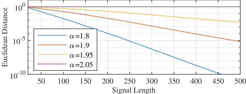
An important statistical analysis goal for super-resolution is to guarantee that an estimator $\widehat{\bm{\theta}}$ remains reasonably close to the ground truth $\bm{\theta}$. A variety of definitions exists in the literature to characterize the stability of super-resolution. All have been shown to be related to the separation parameter $\alpha\triangleq N\Delta(\bm{\tau})$ between the sources, as empirically established by Rayleigh (see e.g. [4]). We give a brief review of the key prior results in this context. When the sources are on a discrete grid, the stability of super-resolution has been shown to be related to the Rayleigh index of the support set [5, 6]. In the last decade, there has been a resurgence in interest in characterizing the resolution limit for sources lying off-the-grid. It is well-established that some instances of super-resolution are statistically unidentifiable under a fixed noise level $\sigma^{2}$ when $N$ grows large if the separation parameter satisfies $\alpha<2$. That is, two ill-separated sets of distinct parameters can lead to arbitrarily close signals. This phenomena is highlighted in Figure 1 for the construction of two signals with $r=N/6$ regularly spaced sources, and can be explained by a phase transition in the conditioning of the matrix $\bm{V}_{0}(\bm{\tau})$ whenever $\alpha<1$ [7, 8]. Additional studies of this property are proposed in the context of colliding pairs of sources [9, 10, 11], and the impact of the bandwidth selection was highlighted in [12].

Figure 1: Euclidean distance $\left\|\bm{x}_{1}-\bm{x}_{2}\right\|_{2}$ between two distinct noiseless signals with separation parameter $\alpha$ and $r=N/6$ sources, for different values of $\alpha$ and of the signal length $N$. Herein, the minimal cross-separation between the sets of locations $\bm{\tau}_{1}$ and $\bm{\tau}_{2}$ composing $\bm{x}_{1}$ and $\bm{x}_{2}$ is set to $\alpha/2$.

Other lines of work aim to characterize instead the resolution limits of specific estimators for the super-resolution problem. For instance, stability guarantees for the MUSIC algorithm are provided as a function of the separation parameter in [13] in the noisy setting. The atomic norm denoiser [14, 15, 16] (a.k.a Beurling-LASSO) can fail to recover $\bm{\theta}$ in the absence of noise whenever $\alpha<2$ [17], and is guaranteed to succeed for $\alpha\geq 2.56$ [14, 18]. Stability and denoising performance under Gaussian white noise are given for a separation $\alpha\geq 5.01$ in [19]. Finally, the support stability [20], ensuring that the estimate $\widehat{\bm{\theta}}$ as the same number of components as of the ground truth $\bm{\theta}$, is established for $\alpha\geq 2.27$ in [21].

II-C Stability of the Fisher Information Matrix

In this paper, we associate the stability of super-resolution with the property of the Fisher information matrix $\bm{J}(\bm{\theta})$ that its smallest eigenvalue is strictly bounded away from $0$. A formal definition of stability is given in the following.

Definition 1 (Stability of the Fisher Information Matrix).

The super-resolution problem is to be stable for a separation parameter $\alpha$ and a dynamic range $\kappa$ if and only if there exists a constant $C(\alpha,\kappa)$ independent of $N$ such that for any set of parameters $\bm{\theta}$ with $N\Delta(\bm{\tau})\geq\alpha$ and $1\leq\min\{\bm{c}\}\leq\max\{\bm{c}\}\leq\kappa$

$$\lambda_{\min}\left(\bm{J}(\bm{\theta})\right)\geq\sigma^{-2}C(\alpha,\kappa).$$ (6)

When read in the light of the CRLB, which states that the covariance $\bm{\Sigma}_{\widehat{\bm{\theta}}}$ of an unbiased estimator $\widehat{\bm{\theta}}$ of $\bm{\theta}$ given $\bm{y}$ is such that $\bm{\Sigma}_{\widehat{\bm{\theta}}}-\bm{J}(\bm{\theta})^{-1}$ is a positive semi-definite Hermitian matrix (see e.g. [22, 23] ), Definition 1 can be reinterpreted in terms of the stability of estimates of linear forms as follows.

Proposition 2 (Bounded CRLB Property).

The super-resolution problem is stable in the sense of Definition 1 if and only if the CRLB of any linear form $z(\bm{\theta})$ on the parameters $\bm{\theta}$ of the kind $z(\bm{\theta})=\bm{q}^{{\mathsf{H}}}\bm{\theta}$ verifies

$$\operatorname{CRLB}(z(\bm{\theta});\bm{y})\leq\sigma^{2}C(\alpha,\kappa)^{-1}\left\|\bm{q}\right\|_{2}^{2},$$ (7)

independently of $N$.

The contrapositive of Proposition 2 induces that the super-resolution problem is not stable if and only if there exists a linear form on the parameters that cannot be reliably estimated in the limit $N\to\infty$. Hence, Definition 1 is stronger than requiring the stability of each individual parameter composing $\bm{\theta}$, which is commonly adopted in the literature. Yet, the notion of stability considered in this work doesn’t guarantee the actual existence of a consistent estimator of a given linear form. The main result of this paper, in the following proposition, establishes stability in the sense of the Fisher information provided that the separation parameter $\alpha$ is sufficiently large.

Proposition 3 (Sufficient Condition for Stability).

Suppose that $\alpha\geq 3.54$, then under Gaussian white noise $\bm{w}\sim\mathcal{N}\left(\bm{0},\sigma^{2}\bm{I}\right)$, and for any $\kappa\geq 1$ the super-resolution problem is stable in the sense of Definition 1. Moreover, there exist a non-decreasing function $h_{-}(\alpha)>0$ and a non-increasing function $h_{+}(\alpha)>0$ such that

$$\lambda_{\min}\left(\bm{J}(\bm{\theta})\right)\geq{} \sigma^{-2}h_{-}(\alpha)>0$$ (8a)

$$\lambda_{\max}\left(\bm{J}(\bm{\theta})\right)\leq{} \sigma^{-2}\kappa^{2}h_{+}(\alpha).$$ (8b)

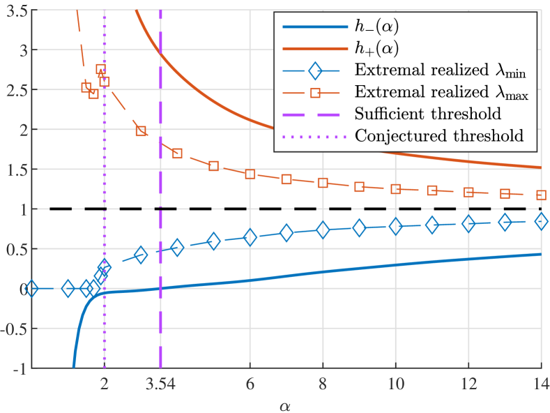
Figure 2 compares the empirical realizations of the extremal eigenvalues of the FIM with the functions $h_{-}(\cdot)$ and $h_{+}(\cdot)$ that will be later constructed in Section III. The evaluation $h_{-}(3.54)>0$ suggests that $\alpha>3.54$ is sufficient to guarantee the stability in the sense of Definition 1, however there is no reason to believe this bound will be tight. Instead, the numerical experiments suggest a phase transition on $\lambda_{\min}\left(\bm{J}(\bm{\theta})\right)$ whenever $\alpha<2$ as the eigenvalue rapidly vanishes to $0$. This observation also coincides with the limit discussed in Section II-B. We leave a sharpening of the bounds for future work. The sequel is devoted to proving Proposition 3.

II-D Proof of Proposition 3

We start the analysis by deriving the FIM $\bm{J}(\bm{\theta})$ (see e.g. [22, 24] of the super-resolution problem (5)

$$\bm{J}(\bm{\theta})=\sigma^{-2}\operatorname{diag}(\bm{1},\bm{c})^{{\mathsf{H}}}\bm{W}(\bm{\tau})^{{\mathsf{H}}}\bm{W}(\bm{\tau})\operatorname{diag}(\bm{1},\bm{c}),$$ (9)

where $\operatorname{diag}(\bm{1},\bm{c})$ denotes the $2r\times 2r$ diagonal matrix whose first $r$ diagonal entries are equal to $1$ and the following $r$ are equal to $\bm{c}$. Some properties of this matrix where studied in [25, 26]. Equation (9) immediately yields that $\bm{J}(\bm{\theta})$ is a positive semi-definite matrix with the following bounds on its extremal eigenvalues

$$\lambda_{\min}\left(\bm{J}(\bm{\theta})\right)\geq{} \sigma^{-2}\min(1,\left|c_{1}\right|,\dots,\left|c_{r}\right|)^{2}\sigma_{\min}\left(\bm{W}(\bm{\tau})\right)^{2}$$

$$\geq{} \sigma^{-2}\sigma_{\min}\left(\bm{W}(\bm{\tau})\right)^{2}$$ (10a)

$$\lambda_{\max}\left(\bm{J}(\bm{\theta})\right)\leq{} \sigma^{-2}\max(1,\left|c_{1}\right|,\dots,\left|c_{r}\right|)^{2}\sigma_{\max}\left(\bm{W}(\bm{\tau})\right)^{2}$$

$$\leq{} \sigma^{-2}\kappa^{2}\sigma_{\max}\left(\bm{W}(\bm{\tau})\right)^{2}.$$ (10b)

Therefore, the crux of the problem consists of ensuring the existence of the two functions $h_{-}(\cdot)$ and $h_{+}(\cdot)$, satifying the conditions stated in Proposition 3 and that minorize (resp. majorize) the quantities $\sigma_{\min}\left(\bm{W}(\bm{\tau})\right)^{2}$ (resp. $\sigma_{\max}\left(\bm{W}(\bm{\tau})\right)^{2}$). This goal is accomplished in the following lemma and proved in Section III after a detour on the Beurling–Selberg extremal approximation problem.

Lemma 4 (Conditioning of $\bm{W}(\bm{\tau})$).

There exist a non-decreasing function $h_{-}(\cdot)$ and a non-increasing function $h_{+}(\cdot)$ such that for any $N$ and any $\bm{\tau}\in{\mathbb{T}}^{r}$ verifying $3.54\leq\alpha\leq N\Delta(\bm{\tau})$, we have the following inequalities

$$\sigma_{\min}\left(\bm{W}(\bm{\tau})\right)^{2}\geq{} h_{-}(\alpha)>0$$ (11a)

$$\sigma_{\max}\left(\bm{W}(\bm{\tau})\right)^{2}\leq{} h_{+}(\alpha).$$ (11b)

The proof of Proposition 3 immediately follows from (10) and Lemma 4. ∎

III Relationship with Bandlimited Approximation

III-A The Beurling–Selberg Box Approximation Problem

Figure 2: The theoretical bounds $h_{-}(\alpha)$ and $h_{+}(\alpha)$ versus the experimental extremal realizations of $\lambda_{\min}\left(\bm{J}(\bm{\theta})\right)$ and $\lambda_{\max}\left(\bm{J}(\bm{\theta})\right)$ when $N\Delta(\bm{\tau})=\alpha$. Parameter values are $N=1001$, $\kappa=1$ and $\sigma^{2}=1$. Experimental results are computed over 200 randomized trials.

The Beurling–Selberg extremal box approximation problem consists of finding a minorant and a majorant to the box function $I_{\alpha}$ that are 1-bandlimited while minimizing the $L_{1}(\mathbb{R})$ distance to $I_{\alpha}$ [27, 28]. Selberg proposed a construction of two approximation functions $B_{-}^{\alpha}(\cdot)$ and $B_{+}^{\alpha}(\cdot)$ by leveraging the properties of Beurling’s extremal approximant of the signum function [29]. In particular, those two functions are said to be extremal in the sense that they achieve $\widehat{B}_{-}^{\alpha}(0)=1-\alpha^{-1}$ and $\widehat{B}_{+}^{\alpha}(0)=1+\alpha^{-1}$ and that any 1-bandlimited minorant $F_{-}^{\alpha}$ (resp. majorant $F_{+}^{\alpha}$) of $I_{\alpha}$ satisfies $\widehat{F}_{-}(0)\leq 1-\alpha^{-1}$ (resp. $\widehat{F}_{+}(0)\geq 1+\alpha^{-1}$). Those properties are particularly interesting because they can be used to bound, in a fairly elegant manner, the singular values of Vandermonde matrices $\bm{V}_{0}(\bm{\tau})$ for any $\bm{\tau}$ with separation parameter $\alpha=N\Delta(\bm{\tau})$ through (see e.g. [30])

$$\sigma_{\min}(\bm{V}_{0}(\bm{\tau}))^{2}\geq{} 1-\alpha^{-1}$$ (12a)

$$\sigma_{\max}(\bm{V}_{0}(\bm{\tau}))^{2}\leq{} 1+\alpha^{-1}.$$ (12b)

Henceforth, given a fixed $\alpha>1$, it is immediately inferred from (12) that $\sigma_{\min}(\bm{V}_{0}(\bm{\tau}))^{2}$ is non-vanishing, and that $\sigma_{\max}(\bm{V}_{0}(\bm{\tau}))^{2}$ is upper bounded by a quantity independent of $N$ for any values of $\alpha>0$.

III-B Higher Order Box Approximations

With the purpose of demonstrating Lemma 4, we introduce a novel higher order box approximation problem, which imposes an additional assumption on the decay rate of the minorizing and majorizing functions of $I_{\alpha}$. The minorant set ${\mathcal{E}}_{\alpha}^{-}$ and minorant set ${\mathcal{E}}_{\alpha}^{+}$ are defined as follows:

Definition 5 (2nd order minorant and majorant set).

Minorant set: Given $\alpha>0$, we let ${\mathcal{E}}_{\alpha}^{-}\subset L_{1}(\mathbb{R})$ the sets of functions $\mathcal{X}_{-}\in L_{1}(\mathbb{R})$ satisfying the following properties:

1. $\mathcal{X}_{-}$ is $1$-bandlimited;

2. $\mathcal{X}_{-}$ minorizes $I_{\alpha}$, i.e. $\mathcal{X}_{-}(t)\leq{}I_{\alpha}(t)$ for all $t$;

3. $\mathcal{X}_{-}(t)=\mathcal{O}(t^{-(3+\varepsilon)})$ when $\left|t\right|\to\infty$ for some $\varepsilon>0$;

4. $\widehat{\mathcal{X}}_{-}^{\prime}(0)={}0$.

Majorant set: Given $\alpha>0$, we let ${\mathcal{E}}_{\alpha}^{+}\subset L_{1}(\mathbb{R})$ the sets of functions $\mathcal{X}_{+}\in L_{1}(\mathbb{R})$ satisfying the following properties:

1. $\mathcal{X}_{+}$ is $1$-bandlimited;

2. $\mathcal{X}_{+}$ majorizes $I_{\alpha}$, i.e. $\mathcal{X}_{+}(t)\geq{}I_{\alpha}(t)$ for all $t$;

3. $\mathcal{X}_{+}(t)=\mathcal{O}(t^{-(3+\varepsilon)})$ when $\left|t\right|\to\infty$ for some $\varepsilon>0$;

4. $\widehat{\mathcal{X}}_{+}^{\prime}(0)={}0$.

We note that, by the Riemann–Lebesgue lemma, the third condition in both cases guarantees the Fourier transform of the functions in ${\mathcal{E}}_{\alpha}^{-}$ and ${\mathcal{E}}_{\alpha}^{+}$ to be at least twice differentiable, which is needed in the fourth condition. The sets proposed in Definition 5 only differ from the original Beurling–Selberg approximation problem in the third and fourth assumptions. However, it can be easily checked from their definitions [29] that $B_{\alpha}^{-}(\cdot)$ and $B_{\alpha}^{+}(\cdot)$ do not belong to ${\mathcal{E}}_{\alpha}^{-}$ and ${\mathcal{E}}_{\alpha}^{+}$, respectively, as they decay at an asymptotic rate $B_{\alpha}^{-}(t)\sim B_{\alpha}^{+}(t)\sim Ct^{-2}$ when $\left|t\right|\to\infty$, thus fail to meet the third assumption.

The following proposition is at the core of the proof of Proposition 3 and establishes a relationship between the functions belonging to the set ${\mathcal{E}}_{\alpha}^{-}$ and ${\mathcal{E}}_{\alpha}^{+}$ and the extremal singular values of the matrix $\bm{W}(\bm{\tau})$.

Proposition 6 (Conditioning of $\bm{W}(\bm{\tau})$ via Bandlimited Functions).

Let $N=2n+1$ be an odd integer. For any fixed $\alpha>0$, let $\bm{\tau}\in{\mathbb{T}}^{r}$, be such that $N\Delta(\bm{\tau})\geq\alpha$. Then, for any function $\mathcal{X}_{-}\in{\mathcal{E}}_{\alpha}^{-}$ and $\mathcal{X}_{+}\in{\mathcal{E}}_{\alpha}^{+}$, we have

$${\sigma_{\min}(\bm{W}(\bm{\tau}))}^{2}\geq{} \min\left\{\alpha^{-1}\widehat{\mathcal{X}}_{-}(0),-\frac{3}{\pi^{2}}\alpha^{-3}\widehat{\mathcal{X}}_{-}^{{\prime\prime}}(0)\right\}$$ (13a)

$${\sigma_{\max}(\bm{W}(\bm{\tau}))}^{2}\leq{} \max\left\{\alpha^{-1}\widehat{\mathcal{X}}_{+}(0),-\frac{3}{\pi^{2}}\alpha^{-3}\widehat{\mathcal{X}}_{+}^{{\prime\prime}}(0)\right\}.$$ (13b)

A few remarks are of order regarding the statement of Proposition 6. The crux of the problem is two fold. First, the extremal singular values can be controlled given the existence of functions within the the sets ${\mathcal{E}}_{\alpha}^{-}$ and ${\mathcal{E}}_{\alpha}^{+}$, hence a strategy to prove Proposition 3 is to show that those two sets are not empty for a large enough value of $\alpha$. Second, noticing that $\widehat{I}_{\alpha}(0)=\int_{\mathbb{R}}I_{\alpha}(t)dt=\alpha$ and ${\widehat{I}_{\alpha}}^{{\prime\prime}}(0)=\int_{\mathbb{R}}-4\pi^{2}t^{2}I_{\alpha}(t)dt=-\frac{\pi^{2}}{3}\alpha^{3}$, the scaling of the bounds (13) can be considered to be tight in the sense that the right sides of both equations with the functions $\mathcal{X}_{-}=\mathcal{X}_{+}=I_{\alpha}$ equal $1$. Hence, better bounds are achieved for functions in ${\mathcal{E}}_{\alpha}^{-}$ and ${\mathcal{E}}_{\alpha}^{+}$ that are close to the box function $I_{\alpha}$. The best bounds on the singular values of the sensitivity matrix $\bm{W}(\bm{\tau})$ in Proposition 6 are provided by the extremal functions that achieve the maximal and minimal values on the right-hand sides of equations (13a) and (13b) respectively. However, to our knowledge, there are no known derivations to date for those extremal functions. We seek to ameliorate that lack in the sequel.

III-C Approximation via Polynomial Transforms

In this section, we construct a pair of suboptimal functions $G_{\alpha}^{-}(\cdot)$ and $G_{\alpha}^{+}(\cdot)$ belonging to the sets ${\mathcal{E}}_{\alpha}^{-}$ and ${\mathcal{E}}_{\alpha}^{+}$, respectively and that achieve a reasonable approximation of the box function $I_{\alpha}$. We proceed by applying a transform ${\mathcal{P}}$ to the Beurling–Selberg extremal functions discussed in III-A which preserves the first and second properties of ${\mathcal{E}}_{\alpha}^{-}$ and ${\mathcal{E}}_{\alpha}^{+}$ in Definition 5 respectively. Mathematically, it is sufficient to ensure that ${\mathcal{P}}$ satisfies the following properties:

1. For any 1-bandlimited function $F$, then ${\mathcal{P}}\{F\}$ is also 1-bandlimited;

2. If $F$ minorizes (resp. majorizes) the box function $I_{\alpha}$ then ${\mathcal{P}}\{F\}$ also minorizes (resp. majorizes) $I_{\alpha}$;

3. If $F(t)\to 0$ at $\left|t\right|\to\infty$ then ${\mathcal{P}}\{F\}(t)=\mathcal{O}(F(t)^{2})$ in the limit $\left|t\right|\to\infty$.

Polynomial transforms are a good fit to achieve those three conditions, since any polynomial $P$ of degree $d$ preserves the spectral support of $F$ through the map ${\mathcal{P}}\{F\}(t)=P(F(\frac{t}{d}))$. It can be checked that, while not unique, the polynomial $P(t)=t^{3}$ is the minimal degree polynomial for which ${\mathcal{P}}$ matches those three properties. This suggests a construction of $G_{\alpha}^{-}(\cdot)$ and $G_{\alpha}^{+}(\cdot)$ as in Lemma 7, whose proof is omitted for brevity.

Lemma 7.

Let $\alpha>0$, and denote by $G_{\alpha}^{-}$ and $G_{\alpha}^{+}$ the functions given by

$$G_{\alpha}^{-}(t) {}\triangleq{\mathcal{P}}\{B_{\alpha/3}^{-}\}(t)={B_{\alpha/3}^{-}(t/3)}^{3}$$ (14a)

$$G_{\alpha}^{+}(t) {}\triangleq{\mathcal{P}}\{B_{\alpha/3}^{+}\}(t)={B_{\alpha/3}^{+}(t/3)}^{3},$$ (14b)

then we have that $G_{\alpha}^{-}\in{\mathcal{E}}_{-}^{\alpha}$ and $G_{\alpha}^{+}\in{\mathcal{E}}_{+}^{\alpha}$.

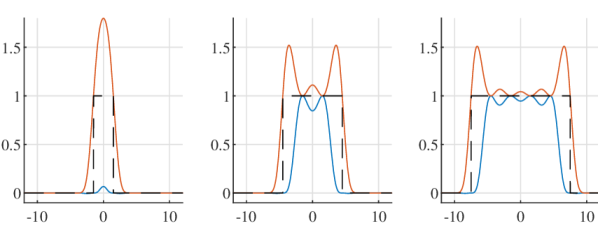
Figure 3 shows the graph of these functions and their Fourier transforms for three different values of the separation parameter $\alpha$.

We now have all the elements to prove Lemma 4 which is integral to the proof of Proposition 3. We let $h_{-}(\alpha)$ and $h_{+}(\alpha)$ be the value of the right-hand side of the bounds (13) applied to the functions $G_{\alpha}^{-}(\cdot)\in{\mathcal{E}}_{\alpha}^{-}$ and $G_{\alpha}^{+}(\cdot)\in{\mathcal{E}}_{\alpha}^{+}$ defined in (14), respectively. The numerical evaluation of those quantity shown in Figure 2 ensures that $h_{-}(\alpha)>0$ whenever $\alpha\geq 3.54$, which concludes on the desired statement. ∎

Figure 3: The graph of the functions $G_{\alpha}^{-}(t)$ (in blue), $G_{\alpha}^{+}(t)$ (in red) and $I_{\alpha}(t)$ (in black dashed lines). Left: $\alpha=3$; Middle: $\alpha=9$; Right: $\alpha=15$

IV Proof of Proposition 6

We focus on proving that (13a) holds, as (13b) can be derived in an analogous manner. Consider a vector $\bm{\tau}\in\mathbb{T}^{r}$ of an arbitrary number $r$ of elements, and let $\alpha=N\Delta(\bm{\tau})$. We fix $\bm{u}_{0},\bm{u}_{1}\in\mathbb{C}^{r}$ and we let by $\bm{u}=[\bm{u}_{0}^{\top},\bm{u}_{1}^{\top}]^{\top}\in\mathbb{C}^{2r}$, the concatenation of the two vectors. Assume that the function $\mathcal{X}_{-}(\cdot)$ is in the set ${\mathcal{E}}_{\alpha}^{-}$. We start by introducing the auxiliary functions $\varphi_{0}(\cdot)$ and $\varphi_{1}(\cdot)$ defined for all $y\in\mathbb{R}$ by

$$\varphi_{0}(y)={} \frac{1}{\sqrt{N}}\sum_{\ell=1}^{r}u_{0,\ell}e^{-i2\pi\tau_{\ell}y}$$ (15a)

$$\varphi_{1}(y)={} -\frac{C_{N}}{\sqrt{N}}\sum_{\ell=1}^{r}u_{1,\ell}i2\pi ye^{-i2\pi\tau_{\ell}y}.$$ (15b)

and let by $S_{p}(\ell,{\ell^{\prime}})$ for $p=0,1,2$ the series

$$S_{p}(\ell,{\ell^{\prime}})={}\sum_{k=-\infty}^{\infty}\mathcal{X}_{-}\left(k\Delta(\bm{\tau})\right)\left(i2\pi k\right)^{p}e^{-i2\pi k(\tau_{\ell}-\tau_{\ell}^{\prime})}.$$ (16)

Given these definitions, we can introduce $\mathcal{X}_{-}$ to minorize the quantity $\left\|\bm{W}(\bm{\tau})\bm{u}\right\|_{2}^{2}$ as follows

$$\left\|\bm{W}(\bm{\tau})\bm{u}\right\|_{2}^{2}={} \sum_{k=-n}^{n}\left|\varphi_{0}(k)+\varphi_{1}(k)\right|^{2}$$

$$={} \sum_{k=-\infty}^{\infty}I_{\alpha}(k\Delta(\bm{\tau}))\left|\varphi_{0}(k)+\varphi_{1}(k)\right|^{2}$$

$$\geq{} \sum_{k=-\infty}^{\infty}\mathcal{X}_{-}\left(k\Delta(\bm{\tau})\right)\left|\varphi_{0}(k)+\varphi_{1}(k)\right|^{2}$$

$$={} \frac{1}{N}\sum_{\ell=1}^{r}\sum_{\ell^{\prime}=1}^{r}u_{0,\ell}u_{0,\ell^{\prime}}S_{0}(\ell,{\ell^{\prime}})$$

$$\quad-\frac{2C_{N}}{N}\Re\left(\sum_{\ell=1}^{r}\sum_{\ell^{\prime}=1}^{r}u_{0,\ell}u_{1,\ell^{\prime}}S_{1}(\ell,{\ell^{\prime}})\right)$$

$$\quad+\frac{{C_{N}}^{2}}{N}\sum_{\ell=1}^{r}\sum_{\ell^{\prime}=1}^{r}u_{1,\ell}u_{1,\ell^{\prime}}S_{2}(\ell,{\ell^{\prime}}),$$ (17)

where the first inequality stems from the fact that $k\Delta(\bm{\tau})\in[-\alpha/2,\alpha/2]$ if and only if $\left|k\right|\leq n$, and the second because $\mathcal{X}_{-}(t)\leq I_{\alpha}(t)$ for all $t\in\mathbb{R}$ by assumption. Moreover, the terms of the series $S_{p}(\ell,{\ell^{\prime}})$ are equivalent to the function $h_{p}:x\mapsto\mathcal{X}_{-}(x\Delta(\bm{\tau})){(i2\pi x)}^{p}e^{-i2\pi x(\tau_{\ell}-\tau_{\ell^{\prime}})}$ when the argument is an integer. By the third assumption in Definition 5, the functions $h_{p}$ are absolutely summable for $p=0,1,2$ with continuous time Fourier transform $\widehat{h}_{p}(u)=\Delta(\bm{\tau})^{-(1+p)}\widehat{\mathcal{X}}_{-}^{(p)}(\Delta(\bm{\tau})^{-1}(u-\tau_{\ell}+\tau_{\ell^{\prime}}))$, which is of finite support by the first assumption and bounded by the third one, therefore also absolutely summable. Hence, the Poisson summation formulae can be applied on the series $S_{p}(\ell,{\ell^{\prime}})$. They yield for all pairs $(\ell,{\ell^{\prime}})\in\left\{1,\dots,r\right\}^{2}$ and all $p=0,1,2$

$$S_{p}(\ell,{\ell^{\prime}})=\Delta(\bm{\tau})^{-(1+p)}\sum_{j=-\infty}^{\infty}\widehat{\mathcal{X}}_{-}^{(p)}\left(\Delta(\bm{\tau})^{-1}(j-\tau_{\ell}+\tau_{\ell^{\prime}})\right).$$ (18)

By our assumption on the separation, we have that $\Delta(\bm{\tau})^{-1}(j-\tau_{\ell}+\tau_{\ell^{\prime}})>1$ for any $j\in\mathbb{Z}$ and any pair $(\ell,{\ell^{\prime}})$ unless $\ell={\ell^{\prime}}$ and $j=0$. As $\mathcal{X}_{-}(\cdot)$ is $1$-bandlimited, we conclude that the terms on the right hand side of (18) are all $0$ unless $\ell={\ell^{\prime}}$ and $j=0$. Thus, (18) reduces for $p=0,1,2$ to

$$S_{p}(\ell,{\ell^{\prime}})=\begin{cases}\Delta(\bm{\tau})^{-(p+1)}\widehat{\mathcal{X}}_{-}^{(p)}\left(0\right)&\text{if }\ell={\ell^{\prime}},\\ 0&\text{otherwise}.\end{cases}$$ (19)

Substituting (19) into (IV) with $\widehat{\mathcal{X}}_{-}^{\prime}(0)=0$, $\frac{C_{N}^{2}}{N}\geq\frac{3}{\pi N^{3}}$ for all $N>1$, and $\alpha=N\Delta(\bm{\tau})$ yields

$$\left\|\bm{W}(\bm{\tau})\bm{u}\right\|_{2}^{2}$$

$$\geq{} \left(N\Delta(\bm{\tau})\right)^{-1}\widehat{\mathcal{X}}_{-}(0)\left\|\bm{u}_{0}\right\|_{2}^{2}-\frac{{C_{N}}^{2}}{N}\Delta(\bm{\tau})^{-3}\widehat{\mathcal{X}}_{-}^{{\prime\prime}}(0)\left\|\bm{u}_{1}\right\|_{2}^{2}$$

$$={} \alpha^{-1}\widehat{\mathcal{X}}_{-}(0)\left\|\bm{u}_{0}\right\|_{2}^{2}-\frac{3}{\pi^{2}}\alpha^{-3}\widehat{\mathcal{X}}_{-}^{{\prime\prime}}(0)\left\|\bm{u}_{1}\right\|_{2}^{2}.$$ (20)

Finally, the definition of the singular value and (IV) imply

$${\sigma_{\min}(\bm{W}(\bm{\tau}))}^{2}={} \min_{\left\|\bm{u}\right\|_{2}^{2}=1}\left\|\bm{W}(\bm{\tau})\bm{u}\right\|_{2}^{2}$$

$$\geq{} \min\left\{\alpha^{-1}\widehat{\mathcal{X}}_{-}(0),-\frac{3}{\pi^{2}}\alpha^{-3}\widehat{\mathcal{X}}_{-}^{{\prime\prime}}(0)\right\},$$ (21)

which yields our desired statement. ∎

V Conclusion and Future Work

In the present work, we considered the stability of the Fisher information matrix of the super-resolution problem in the regime where the separation between the sources is inversely proportional to the number of measurements. Proposition 3 establishes the stability of the FIM whenever the separation parameter verifies $\alpha\geq 3.54$. This result was demonstrated by unveiling in Proposition 6 a connection between the singular values of the sensitivity matrix and the solutions of a novel Beurling–Selberg type approximation problem, for which we derived a pair of sub-optimal solutions. We leave for a sequel the study of the extremal solutions to this approximation problem in the hope of guaranteeing the stability of the FIM up to the conjectured threshold $\alpha>2$.

References

- [1] J. Lindberg “Mathematical concepts of optical superresolution” In Journal of Optics - IOP Publishing 14.8, 2012, pp. 83001
- [2] Sang-Hyuk Lee, Jae Yen Shin, Antony Lee and Carlos Bustamante “Counting single photoactivatable fluorescent molecules by photoactivated localization microscopy (PALM)” In Proceedings of the National Academy of Sciences 109.43 National Acad Sciences, 2012, pp. 17436–17441
- [3] J-J Fuchs “Sparsity and uniqueness for some specific under-determined linear systems” In Proceedings of IEEE International Conference on Acoustics, Speech, and Signal Processing 5 IEEE, 2005, pp. v–729
- [4] Max Born and Emil Wolf “Principles of optics: electromagnetic theory of propagation, interference and diffraction of light” Elsevier, 2013
- [5] David L Donoho “Superresolution via sparsity constraints” In SIAM journal on mathematical analysis 23.5 SIAM, 1992, pp. 1309–1331
- [6] Laurent Demanet and Nam Nguyen “The recoverability limit for superresolution via sparsity” In arXiv preprint arXiv:1502.01385, 2015
- [7] Céline Aubel, David Stotz and Helmut Bölcskei “A theory of super-resolution from short-time Fourier transform measurements” In Journal of Fourier Analysis and Applications 24.1, 2018, pp. 45–107
- [8] Ankur Moitra “Super-resolution, extremal functions and the condition number of Vandermonde matrices” In Proceedings of the forty-seventh annual ACM symposium on Theory of computing ACM, 2015, pp. 821–830
- [9] Dmitry Batenkov, Gil Goldman and Yosef Yomdin “Super-resolution of near-colliding point sources” In Information and Inference: A Journal of the IMA 10.2 Oxford University Press, 2021, pp. 515–572
- [10] Stefan Kunis and Dominik Nagel “On the condition number of Vandermonde matrices with pairs of nearly-colliding nodes” In Numerical Algorithms 87.1 Springer, 2021, pp. 473–496
- [11] Benedikt Diederichs “Well-Posedness of Sparse Frequency Estimation” In arXiv preprint arXiv:1905.08005, 2019
- [12] Dmitry Batenkov, Ayush Bhandari and Thierry Blu “Rethinking super-resolution: the bandwidth selection problem” In ICASSP 2019-2019 IEEE International Conference on Acoustics, Speech and Signal Processing (ICASSP), 2019, pp. 5087–5091 IEEE
- [13] Wenjing Liao and Albert Fannjiang “MUSIC for single-snapshot spectral estimation: Stability and super-resolution” In Applied and Computational Harmonic Analysis 40.1 Elsevier, 2016, pp. 33–67
- [14] Emmanuel J Candès and Carlos Fernandez-Granda “Towards a Mathematical Theory of Super-resolution” In Communications on Pure and Applied Mathematics 67.6, 2014, pp. 906–956
- [15] Yohann De Castro and Fabrice Gamboa “Exact reconstruction using Beurling minimal extrapolation” In Journal of Mathematical Analysis and Applications 395.1, 2012, pp. 336–354 DOI: 10.1016/j.jmaa.2012.05.011
- [16] Y. Chi and M. Ferreira Da Costa “Harnessing Sparsity Over the Continuum: Atomic norm minimization for superresolution” In IEEE Signal Processing Magazine 37.2, 2020, pp. 39–57 DOI: 10.1109/MSP.2019.2962209
- [17] Maxime Ferreira Da Costa and Wei Dai “A Tight Converse to the Spectral Resolution Limit via Convex Programming” In 2018 IEEE International Symposium on Information Theory (ISIT), 2018, pp. 901–905 DOI: 10.1109/ISIT.2018.8437490
- [18] Carlos Fernandez-Granda “Super-resolution of point sources via convex programming” In Information and Inference 5.3, 2016, pp. 251–303 DOI: 10.1093/imaiai/iaw005
- [19] Qiuwei Li and Gongguo Tang “Approximate support recovery of atomic line spectral estimation: A tale of resolution and precision” In Applied and Computational Harmonic Analysis, 2018
- [20] Vincent Duval and Gabriel Peyré “Exact support recovery for sparse spikes deconvolution” In Foundations of Computational Mathematics 15.5, 2015, pp. 1315–1355 DOI: 10.1007/s10208-014-9228-6
- [21] M. Ferreira Da Costa and Y. Chi “On the Stable Resolution Limit of Total Variation Regularization for Spike Deconvolution” In IEEE Transactions on Information Theory, 2020
- [22] Louis L Scharf and L Todd McWhorter “Geometry of the Cramér-Rao bound” In Signal Processing 31.3 Elsevier, 1993, pp. 301–311
- [23] S.. Smith “Statistical resolution limits and the complexified Cramér-Rao bound” In IEEE Transactions on Signal Processing 53.5, 2005, pp. 1597–1609
- [24] Pooria Pakrooh et al. “Analysis of Fisher information and the Cramér–Rao bound for nonlinear parameter estimation after random compression” In IEEE Transactions on Signal Processing 63.23 IEEE, 2015, pp. 6423–6428
- [25] Lei Li and Terence P Speed “Parametric deconvolution of positive spike trains” In The Annals of Statistics 28.5 Institute of Mathematical Statistics, 2000, pp. 1279–1301
- [26] Thierry Blu et al. “Sparse sampling of signal innovations” In IEEE Signal Processing Magazine 25.2 IEEE, 2008, pp. 31–40
- [27] Atle Selberg “Collected papers. II” Springer, 2014
- [28] P Akhilesh and D Ramana “A remark on the Beurling-Selberg function.” In Acta Mathematica Hungarica 139.4, 2013
- [29] Jeffrey D Vaaler “Some extremal functions in Fourier analysis” In Bulletin (New Series) of The American Mathematical Society 12.2 American Mathematical Society, 1985, pp. 183–216
- [30] Céline Aubel and Helmut Bölcskei “Vandermonde matrices with nodes in the unit disk and the large sieve” In Applied and Computational Harmonic Analysis 47.1 Elsevier, 2019, pp. 53–86