Nonequilibrium topological spin textures in momentum space

Abstract

Nonequilibrium quantum dynamics of many-body systems is the frontier of condensed matter physics; recent advances in various time-resolved spectroscopic techniques continue to reveal rich phenomena. Angle-resolved photoemission spectroscopy (ARPES) as one powerful technique can resolve electronic energy, momentum, and spin along the time axis after excitation. However, dynamics of spin textures in momentum space remains mostly unexplored. Here we demonstrate theoretically that the photoexcited surface state of genuine or magnetically doped topological insulators shows novel topological spin textures, i.e., tornado-like patterns, in the spin-resolved ARPES. We systematically reveal its origin as a unique nonequilibrium photoinduced topological winding phenomenon. As all intrinsic and extrinsic topological helicity factors of both material and light are embedded in a robust and delicate manner, the tornado patterns not only allow a remarkable tomography of these important system information, but also enable various unique dichroic topological switchings of the momentum-space spin texture. These results open a new direction of nonequilibrium topological spin states in quantum materials.

Introduction

The recent decade has witnessed significant advances in the detection means of ultrafast light-induced phenomena[1, 2] in terms of time-resolved spectroscopic techniques including angle-resolved photoemission spectroscopy (ARPES)[3, 4, 5], terahertz pump-probe scanning-tunneling microscopy and optical conductivity measurement[6, 7, 8, 9], etc. Unprecedented precise access into the inherently time-dependent phenomena is beneficial and important to both the fundamental interest in nonequilibrium physics and the practical connection to ultrafast manipulation of novel quantum degrees of freedom towards application[10, 11, 12]. To this end, a robust low-dimensional nontrivial system would be a versatile playground for such surface-sensitive pump-probe-type investigation. The protected surface state of topological insulator fits into this role for its long enough mean free path and lifetime and also for excluding the insulating and spin-degenerate bulk influence[13, 14, 15]. Tunable exchange gap from controlling magnetic doping further allows for demonstrating both massless and massive Dirac physics[16, 17, 18, 19].

However, nonequilibrium spin dynamics is usually studied in time domain or real space only[20, 21]. For the surface state, it has been focused on the equilibrium spin-orbit coupling features[22, 23] and the photodriven steady-state or highly pumped charge current responses[24, 25, 26, 27, 28, 29]. The nonequilibrium phenomena of light-matter interaction in this system remain largely buried partially due to the little appreciated spin-channel physics. In fact, such information connects well to the state-of-art experimental reach, e.g., spin-resolved ARPES (SARPES) has been established in equilibrium and as well extended to time-dependent measurement well below picosecond resolution[22, 23, 30, 31, 32, 33, 34, 5]. As an example of the new front of nonequilibrium quantum dynamics of topological matters, we draw attention to this highly informative time-dependent signal in an optical pump-probe experiment upon the surface state.

In particular, we simulate the irradiation of a terahertz short laser pulse, which can be either linearly polarized (LP) or circularly polarized (CP)[35], to pump across the exchange gap; then detect the SARPES signal after a controllable delay time with a probe pulse. Apart from possible resonant transition, virtual excitation at the early stage of time evolution is a purely quantum mechanical effect and can turn the system into a many-particle coherent nonequilibrium state. Surprisingly, the SARPES signal exhibits robust and topological tornado-like spiral structures in the two-dimensional (2D) momentum ${\bm{k}}$-space, which can be characterized by topological indices. This happens in both the normal and in-plane spin channels and embeds a delicate relation to three helicity factors determining the pumped system: intrinsic helicity of the surface state $\chi=\pm 1$, sign of the Dirac mass $\nu=\operatorname{sgn}{(m)}$, and extrinsic helicity $\tau=0,\pm 1$ respectively for LP and right or left CP lights. Depending on these, the novel tornado-like responses can dichotomously change characteristic winding senses and even dichroically switch between topological and trivial as a $\mathbb{Z}_{2}$-like topological optical activity.

Figure 1: Nonequilibrium spin-resolved ARPES (SARPES) signals in the $(\varepsilon,k_{x})$-plane. $P_{0},P_{1},P_{2},P_{3}$ successively in the density $\rho$ and spin ${\bm{S}}$ channels of a magnetic topological insulator surface state at three different times. White dashed curves in panels (a1,b1,c1) indicate the surface state band dispersion. The band broadening originates from finite probe pulse width. Parameters are $\chi=\tau=1,t_{0}=t_{\mathrm{pb}}=3,\Omega=1.2,v=1,m=0.4,A_{0}=0.1,k_{y}=0.01,\beta=50,\mu=0,e=\hbar=k_{B}=1$. (a) $t=-60$ signal before pump pulse irradiation exhibits equilibrium response: only lower band is visible due to relatively low temperature specified by $\beta=1/(k_{B}T)$ and in-gap chemical potential. The $90$-degree out-of-phase spin-momentum locking manifests in the spin channels: $P_{1}$ is weak compared to others due to small $k_{y}$; $P_{2}$ reverses sign between positive and negative $k_{x}$-axis; $P_{3}$ is made finite purely by the finite exchange gap. (b) At $t=15$ after the pump pulse centered at $t=0$ almost fully decays, resonant real transition appears as two spots in the upper band in $P_{0}$. The spin channels exhibit a signal hot region centered at $\varepsilon=0$ and $k_{x}=0$, which is oscillatory in time and momentum. This is clearly seen in $P_{1}$ for the weak background from real band occupations, compared to $P_{2},P_{3}$. (c) At a later time $t=24$, while the density channel remains nearly time-independent after the pumping process, the hot region signals in the spin channel evolve in time with increasing fine structures, implying that it originates mainly from virtual excitations and the coherent quantum oscillation correlated in momentum space.

Results

Model and time evolution

We consider the 2D massive Dirac model and henceforth set $\hbar=1$

$$H_{0}({\bm{k}})={\bm{d}}({\bm{k}})\cdot{\bm{\sigma}}=v(k_{x}\sigma_{2}-\chi k_{y}\sigma_{1})+m\sigma_{3}$$ (1)

to represent the surface state with spin Pauli matrices $(\sigma_{0},{\bm{\sigma}})=(I,\sigma_{1},\sigma_{2},\sigma_{3})$. We include the $\chi=-1$ case possible when $C_{n>2}$ rotational symmetries are broken. The two bands $\varepsilon_{{\bm{k}}\pm}=d_{0}(k)\pm d({\bm{k}})$ if we include the spin-independent quadratic term $d_{0}(k)\sigma_{0}$, which is henceforth dropped as it does not affect spin channel response from interband transitions. The hexagonal warping strength $c_{6}$ measured in the dimensionless quantity $c_{6}k_{0}^{2}/v\ll 1$ makes it negligible with the characteristic wavenumber $k_{0}$ introduced later[36, 37]. Therefore, our prediction is fully based on the leading order response in real systems. The ARPES light source typically bears a beam spot size $10\textrm{--}100\mathrm{\mu m}$ upon the sample[1, 35, 38, 5], which requests one to consider physical phenomena at the optical long-wavelength limit as the experimentally most relevant scenario, in contrast to the otherwise interesting space-resolved nano-ARPES or scanning Kerr magnetooptic microscopy study[39, 40, 41]. We thus introduce a spatially uniform Gaussian vector potential for the pump pulse vertically shone onto the $xy$-plane ${\bm{A}}(t)=A_{0}\exp(-t^{2}/2t_{0}^{2})\left[\hat{x}\cos\Omega t+\tau\,\hat{y}\sin\Omega t\right]$, where $\tau=0,\pm 1$ and $t_{0}$ the temporary width. The conserved momentum enables us to derive the full electromagnetically coupled Hamiltonian from Peierls substitution

$$\hat{H}(t)=\sum_{\bm{k}}\psi^{\dagger}({\bm{k}})\left[H_{0}({\bm{k}})+e\partial_{{\bm{k}}}H_{0}({\bm{k}})\cdot{\bm{A}}(t)\right]\psi({\bm{k}})$$ (2)

with $\psi({\bm{k}})=(\psi_{{\bm{k}}\uparrow},\psi_{{\bm{k}}\downarrow})^{\mathrm{T}}$. The time-dependent spinor operator $\psi_{{\bm{k}}\alpha}(t)$ for $\alpha=\uparrow/\downarrow$ can be obtained via the equation of motion, which relates to the double-time matrix removal Green’s function with nonequilibrium occupation and excitation information $G_{\alpha\beta}^{<}({\bm{k}},t_{1},t_{2})=\mathrm{i}\langle\psi_{{\bm{k}}\beta}^{\dagger}(t_{2})\psi_{{\bm{k}}\alpha}(t_{1})\rangle$[42, 43] (see Methods).

Time-dependent SARPES signal

We generalize the time-resolved ARPES theory to obtain the time-dependent SARPES intensity matrix[44, 45] $P(\varepsilon,{\bm{k}},t)=-\mathrm{i}\int\mathrm{d}t_{1}\mathrm{d}t_{2}\,\mathrm{e}^{\mathrm{i}\varepsilon(t_{1}-t_{2})}s(t_{1}-t)s(t_{2}-t)G^{<}({\bm{k}},t_{1},t_{2})$ with $s(t)=(2\pi t_{\mathrm{pb}}^{2})^{-\frac{1}{2}}\mathrm{e}^{-t^{2}/2t_{\mathrm{pb}}^{2}}$ the isotropic probe pulse of width $t_{\mathrm{pb}}$ and the spin-polarized photocurrent intensity $I_{\alpha}\propto P_{\alpha\alpha}$ (see Supplementary Note 1). Then we define

$$P_{i}(\varepsilon,{\bm{k}},t)=\,\mathrm{Tr}[\sigma_{i}P(\varepsilon,{\bm{k}},t)],\qquad i=0,1,2,3$$ (3)

successively for the density and three spin channels to be our main focus since the SARPES polarization reads, e.g., for $z$-direction, $\mathrm{P}_{z}=\frac{I_{\uparrow}-I_{\downarrow}}{I_{\uparrow}+I_{\downarrow}}=\frac{P_{3}}{P_{0}}$. As we mainly consider a probe pulse well separated from the pump pulse ($t\gg t_{0}$), we can stick to the present Hamiltonian gauge and are free from gauge invariance issue[46, 47].

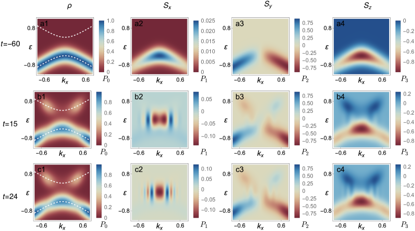
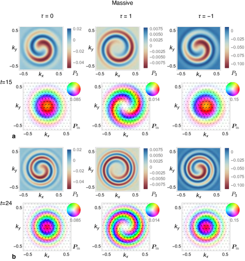
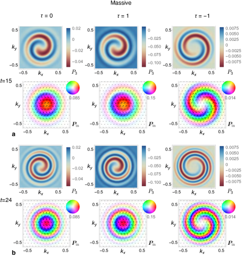
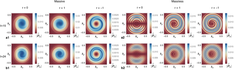
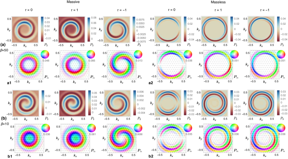
The pump field renders the original Dirac bands no longer eigenstates and occupation can in general change: in the $(\varepsilon,{\bm{k}})$-hyperplane, not only on-resonance real transition can happen when the gap $\Delta=2m<\Omega$, which is the case shown in Fig. 1, but also off-resonance virtual excitations significantly contribute, constituting a transient redistribution along the $\varepsilon$-axis per the particle conservation as a sum-rule-like constraint. After the pump field fully decays, Dirac bands return to be eigenstates. For the density channel, shown in Figs. 1(a1,b1,c1), this implies that, except for resonant interband transition, the signal should mostly become stable after the pumping transients. However, in the spin channel pumping has already left relics of light-matter interaction. Each momentum accommodates a two-level system and is subject to the common photoexcitation. This leads to a highly nontrivial correlation of excited spin-orbit-coupled states in ${\bm{k}}$-space as the central cause of the SARPES tornado textures discussed below. Indeed, collective quantum oscillation effect can emerge near some hot region in the $(\varepsilon,{\bm{k}})$-hyperplane of SARPES, centered at the band midpoint as shown in Figs. 1(b2-4,c2-4). This is because the spin channel extracts the Rabi-like oscillatory information due to interband coherence even as $\hat{H}$ loses time-dependence after the pump pulse. Note also that, as is physically originated from the spin-channel interband quantum oscillation, the real resonant pumping, if any, is insignificant for the hot region signals, which will also become clear later with the analytical result (6).

The probe pulse width $t_{\mathrm{pb}}$ is a double-edged sword per the uncertainty relation: smaller $t_{\mathrm{pb}}$ gives better time resolution but less energy resolution and vice versa. It thus broadens the transient process and smears the SARPES energy levels. Futhermore, certain amount of relaxed energy conservation $\delta\varepsilon\sim 2\pi/t_{\mathrm{pb}}$ and the associated momentum range $\delta k\propto\delta\varepsilon/v$ can actually enhance the signal from off-resonance oscillations and provide the hot region characteristic scales, because energy-sharp bands are incapable of capturing the quantum oscillations. Certainly, too poor energy resolution would otherwise mix contributions, for instance, from both the lower band and the possible higher occupation due to resonant transition. We also emphasize that this quantum nonequilibrium phenomenon goes beyond the semiclassical picture[48]: neither the pumping process nor the interband coherent dynamics at any time can be captured by the wavepacket description within a single band. Direct evidence is the anomalous tornado rotation as quasiparticle trajectory, which is otherwise not expected after the driving electric field in the pump pulse dies out.

Figure 2: Nonequilibrium tornado-like responses in the $(k_{x},k_{y})$-plane. Equilibrium response subtracted SARPES signals (normal-direction $P_{3}$ and in-plane ${\bm{P}}_{\mathrm{in}}=(P_{1},P_{2})$) at (a) $t=15$ (b) $t=24$ after the pump pulse. Energy cut at band midpoint $\varepsilon=0$ is adopted without loss of generality. (a1,b1) Positive mass ($\nu=1$) and (a2,b2) massless case for fixed surface state helicity $\chi=1$. Pump light dependence ($\tau=0,\pm 1$ for LP along $x$-axis and right/left CP) displayed across the columns. Scalar $P_{3}$ plotted for spin-$S_{z}$ signal. In-plane spin orientation angle $\phi=\tan^{-1}{{\bm{P}}_{\mathrm{in}}}$ plotted according to the rainbow color wheel inset; magnitude $|{\bm{P}}_{\mathrm{in}}|$ shown in opacity with maximal $|{\bm{P}}_{\mathrm{in}}|$ indicated below each color wheel. Selected ${\bm{P}}_{\mathrm{in}}$ vector arrows are shown with corresponding magnitude and orientation. See Fig. 3(d) for enlarged illustration. Topological tornado-like spirals appear except the gapless case under LP light. As time elapses, from (a) to (b), tornadoes evolve and rotate and more tornado arms will be accommodated within a fixed ${\bm{k}}$-space region. Tornado responses as the distinguishing feature in relation to all three helicity factors are summarized in Table. 1. Dichroic $P_{3}$-tornado switching helicity with different CP lights [(a1,b1) $\tau=\pm 1$ case of $P_{3}$] is in stark contrast to the $\mathbb{Z}_{2}$-like ${\bm{P}}_{\mathrm{in}}$-tornado, which appears only under one particular CP light in the gapful case [(a1,b1) $\tau=-1$ case of ${\bm{P}}_{\mathrm{in}}$]. $\phi$ in the gapless case exhibits $\pi$-jump, due to vanishing ${\bm{P}}_{\mathrm{in}}$, along the radial direction once it goes across a spiral arm [(a2,b2) case of ${\bm{P}}_{\mathrm{in}}$]. Parameters same as Fig. 1.

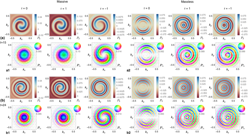
Nonequilibrium tornado responses

Figure 3: Topological tornado indices illustrated in representative cases. Parameters same as Fig. 2(a1) massive case at $t=15$. Scale legends are omitted for simplicity as they are unimportant for the robust tornado features. The spiral winding $W_{s}$ is common for scalar signal (a) $P_{3}$ for $\tau=1$ or (b) $|{\bm{P}}_{\mathrm{in}}|$ for $\tau=-1$ and vectorial in-plane signal (c) ${\bm{P}}_{\mathrm{in}}$ for $\tau=-1$. $W_{s}$ determines the tornado spiral helicity $\Xi_{s}=\operatorname{sgn}{W_{s}}$ and the number $\mathcal{R}_{s}=|W_{s}|$ of repeating spiral arms. For the vectorial signal, more specific radial ordering $\mathcal{K}$ and azimuthal winding $w_{\phi}$ also exist and are combined to give $W_{s}$. (c) shows the counterclockwise circle $C_{k}$ used in defining winding numbers. (d) zooms in the top right quadrant of (c) and exemplifies a particular vector ${\bm{P}}_{\mathrm{in}}$ and its orientation angle $\phi$ together with the rainbow color wheel inset.

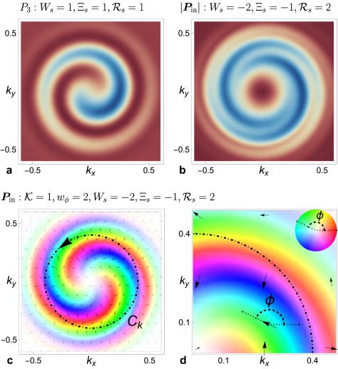
The most interesting information lies in the ${\bm{k}}$-space spin texture ${\bm{P}}(\varepsilon,{\bm{k}},t)=(P_{1},P_{2},P_{3})$ within an energy slice in the hot region, where robust tornado-like structures widely appears as shown in Fig. 2 (see S1 S2 S3 for cases with different $\chi,\nu$). Such energy-momentum hot region lies in general away from where resonant real transitions happen since the tornado mainly originates from coherent virtual excitations, which will be seen also from analytical results. As aforementioned, there are three helicity factors $\chi,\nu,\tau$ at play during the light-matter interaction, for which the subsequent nonequilibrium tornado response turns out to be an exceptionally apt and reliable bookkeeper. For any tornado pattern, one can intuitively identify the rotation sense helicity $\Xi_{s}=\pm 1$ of the spiral and the number $\mathcal{R}_{s}$ of repeating spiral arms. Practically, $\Xi_{s}=\operatorname{sgn}[\partial k^{*}/\partial\theta_{\bm{k}}]$ with $\theta_{\bm{k}}$ the azimuthal angle of ${\bm{k}}$ and $k^{*}(\theta_{\bm{k}})$ any polar-coordinate contour line in a spiral arm. These two lead to the universal topological spiral winding number

$$W_{s}=\Xi_{s}\mathcal{R}_{s}.$$ (4)

We exemplify these quantities in Fig. 3. For the in-plane orientation $\phi({\bm{k}})=\tan^{-1}{\bm{P}}_{\mathrm{in}}({\bm{k}})$ of the vector field ${\bm{P}}_{\mathrm{in}}=(P_{1},P_{2})$, $W_{s}$ is readily determined by a combination of $\phi$’s radial and azimuthal variation. $\phi({\bm{k}})$ has a definite ordering, $\mathcal{K}=\operatorname{sgn}(\partial_{k}\phi)$, i.e., the rainbow order along the radius in our illustration. The latter is encoded in a topological circular winding number

$$w_{\phi}=\frac{1}{2\pi}\int_{C_{k}}\mathrm{d}{\bm{k}}\cdot\nabla\phi({\bm{k}})$$ (5)

along a counterclockwise circle $C_{k}$ of any radius $k$ in the 2D ${\bm{k}}$-plane. We hence obtain $W_{s}=-\mathcal{K}w_{\phi}$. Note that, depending on the helicity factors, any two of $\mathcal{K},w_{\phi},W_{s}$ can switch sign independently and the two together determine the topological tornado features. On the other hand, for a scalar field with less information, $P_{3}$ or the amplitude $|{\bm{P}}_{\mathrm{in}}|$, only Eq. (4) is relevant and suffices to specify the tornado pattern, which will later be cast in the same form as Eq. (5) from the analytical result.

Table. 1 summarizes the correspondence between the three helicity factors and five related aspects in $P_{3}$ and ${\bm{P}}_{\mathrm{in}}$. The dichroic strong/weak response strength of $P_{3}$ happens with CP light and can be owed to the dipole interband matrix element $\braket{\pm}{\hat{{\bm{v}}}}{\mp}$ involving the orbital magnetic moment $\mathcal{M}({\bm{k}})$[49, 50]. Besides, the $P_{3}$-tornado displays the extrinsic (intrinsic) helicity factor(s) pinpointedly under CP (LP) light pumping. This is understood as the intrinsic helicities are only transparent under the non-chiral LP light and otherwise overridden by the extrinsic electric field rotation driving the electrons. These features constitute a perfect tomography of the defining helicity parameters of the surface state system and the light-matter interaction, especially given the topological robustness characterized by $W_{s}$.

However, although tornadoes always exist in the spin-$S_{z}$ signal $P_{3}$, their appearance in the vectorial orientation $\phi({\bm{k}})$ of ${\bm{P}}_{\mathrm{in}}$ is intriguingly selective. Considering the nonequilibrium excitations due to the pumping, its winding number two presumably reflects the Berry phase contribution from both particle and hole. Most significantly, other parameters provided, either $W_{s}$ or $w_{\phi}$ is nonzero only for one type of CP light, making it a novel topological optical activity: dichroic $\mathbb{Z}_{2}$ topological switching between trivial and nontrivial nonequilibrium responses. Therefore, in addition to the helicity $\Xi_{s}=\pm 1$ dichroic switching of $P_{3}$, the $\mathbb{Z}_{2}$ ${\bm{P}}_{\mathrm{in}}$-response hints at further possibly interesting ultrafast spintronic applications taking advantage of the two types of all-optical two-state control.

In fact, the interplay between extrinsic and intrinsic factors can also be unmasked through the amplitude $|{\bm{P}}_{\mathrm{in}}|$, which exactly follows the response of $P_{3}$ except a doubled $W_{s}$, as exemplified in Fig. 3(b). Unlike the $P_{3}$-response, aforementioned $\phi$’s radial variation $\mathcal{K}$ is purely locked to $\nu$, giving rise to a stable characterization of the sign of Dirac mass independent of any other factors. Lastly, in the case of negative spin-orbit coupling that reverses the sign of Fermi velocity $v$, only a sign change of ${\bm{P}}_{\mathrm{in}}$ is induced in the in-plane response that does not alter any topological features[51, 52].

The massless side of the phenomena is presumably simpler: every dichotomous response no longer exists if directly involving the mass sign $\nu$, and only CP light remains active. The purely dichroic tornado in $P_{3}$ and $|{\bm{P}}_{\mathrm{in}}|$ persists. Vanishing mass, however, leads to singular $\pi$-jump in the in-plane $\phi$ along radial direction [e.g., Fig. 2(a2)]: the tornado trajectory of such domain wall follows the driven dichroic helicity. $\phi$’s variation, i.e., color rotation along the tornado arms, naturally inherits the intrinsic winding sense $\chi$ as in the massive case although the domain wall prevents from completing a quantized winding. The apparent distinction between the massive and massless responses is smoothly connected in the crossover regime $|m|t\sim 1$. For instance, tiny amount of magnetic doping ($|m|t\ll 1$) follows the massless behavior and the late-time response of finite doping ($|m|t\gg 1$) generally obeys the massive response pattern.

		massive		massless
normal $P_{3}$ & in-plane $|{\bm{P}}_{\mathrm{in}}|$	response strength	$\quad\chi\nu\tau$	$\quad\tau=\pm 1$	-	-
	spiral winding $W_{s}$ ($\times 2$ for $|{\bm{P}}_{\mathrm{in}}|$)	$\quad\chi\nu$	$\quad\tau=0$	-	$\quad\tau=0$
		$\quad\tau$	$\quad\tau=\pm 1$	$\quad\tau$	$\quad\tau=\pm 1$
in-plane $\phi=\tan^{-1}({\bm{P}}_{\mathrm{in}})$	radial $\mathcal{K}=\operatorname{sgn}(\partial_{k}\phi)$	$\quad\nu$	-	-	-
	circular winding $w_{\phi}$	$\quad 0$	$\quad\chi\nu\tau=0,1$	$\quad\chi^{*}$	$\quad\tau=0$
		$\quad 2\chi$	$\quad\chi\nu\tau=-1$		$\quad\tau=\pm 1$
	spiral winding $W_{s}=-\mathcal{K}w_{\phi}$	$\quad 0$	$\quad\chi\nu\tau=0,1$	-	$\quad\tau=0$
		$\quad 2\tau$	$\quad\chi\nu\tau=-1$	$\quad\tau^{*}$	$\quad\tau=\pm 1$

Table 1: Correspondence between nonequilibrium topological tornado responses and three system helicity factors – intrinsic surface state helicity $\chi=\pm 1$, sign of Dirac mass $\nu=\pm 1$ or massless case without $\nu$, and extrinsic pump light helicity $\tau=0,\pm 1$. Spin-$S_{z}$ signal $P_{3}({\bm{k}})$ and in-plane signal amplitude $|{\bm{P}}_{\mathrm{in}}|$ show the same dichroism in both the strong or weak ($\pm 1$) response strength and the ${\bm{k}}$-space tornado helicity $\Xi_{s}=\operatorname{sgn}{W_{s}}=\pm 1$, although spiral winding $W_{s}$ and hence arm number $\mathcal{R}_{s}=|W_{s}|$ are doubled for $|{\bm{P}}_{\mathrm{in}}|$. The strength response combines all three factors; $W_{s}$ is purely driven by extrinsic CP light while it manifests intrinsic factors under LP light. (Massive case $|{\bm{P}}_{\mathrm{in}}|$-tornado can be less discernible in Fig. 2 due to obstruction from color, but is otherwise observable when plotted separately. See Fig. 3(b) and S4.) In-plane vectorial tornado signal ${\bm{P}}_{\mathrm{in}}({\bm{k}})$ contains more information than scalar signals. The azimuthal angle $\phi({\bm{k}})$, encoding the in-plane orientational variation, exhibits a mass-only dependence of $\mathcal{K}$ along the radial direction. Two other related topological winding numbers $w_{\phi},W_{s}$ exist in the massive case and exhibit a $\mathbb{Z}_{2}$ topological trivial-nontrivial switching for all three factors. $W_{s}$, common in both scalar and vectorial signals, is driven by CP light ($\tau$) when tornado exists, as it shares the same physical meaning of describing spiral rotation. ($*$) Singular $\pi$-jump domain wall of $\phi$, a double-armed helicity-$\tau$ tornado, disables $\mathcal{K},w_{\phi},W_{s}$ in the massless case; $\chi$ determines $\phi$’s winding sense away from the domain wall for any light polarization.

Physical mechanism of tornado

As seen previously, instead of the possible real transition, virtual excitations giving rise to off-diagonal coherence of electronic density matrix contribute to the tornado formation. On top of the ground-state spin-momentum-locked concentric ring-like spin texture, we can intuitively view the optical pumping as producing coherent ${\bm{k}}$-dependent matrix element and concomitant phase accumulation: the nontrivially correlated phase along the ring rotates the spins to yield the tornado. This in a way resembles the gas laser, where independent molecules are excited and brought in a correlated nontrivial coherence by the light working as glue. To gain quantitative insight into the nonequilibrium response, we resort to the Keldysh formalism to calculate the crucial $G^{<}({\bm{k}},t_{1},t_{2})$ and hence the SARPES signal Eq. (3). In this regard, the linear response is tractable and particularly useful as it captures leading virtual excitations but discards real transitions, given the realistic pumping field is often well within the linear response regime. In addition, since the tornado response is of stable topological nature, the features can persist even beyond as the above relatively larger field calculation confirms.

The analytical result matches the previous exact calculation in the linear response regime as it should do. For the late-time behavior of our main interest, we can derive an exceptionally simple expression for general two-band systems: $P_{0}^{(1)}(\varepsilon,{\bm{k}},t)\equiv 0$ and

$$\begin{split}{\bm{P}}^{(1)}(\varepsilon,{\bm{k}},t)&=\frac{2A_{0}W(k)}{d^{2}}\left(f_{\varepsilon_{{\bm{k}}-}}-f_{\varepsilon_{{\bm{k}}+}}\right)F(\varepsilon)\tilde{{\bm{P}}}({\bm{k}},t)\end{split}$$ (6)

with $f_{\varepsilon_{{\bm{k}}\pm}}$ the Fermi function for the upper and lower bands $\varepsilon_{{\bm{k}}\pm}$. The vanishing result in the density channel confirms the recovery of stable energy eigenstates after the pump’s influence. For the spin channel, the dependence on occupation difference in the two bands indicates the optical inertness of both bands being empty or filled. The energy function in a Gaussian form $F(\varepsilon)=\mathrm{e}^{-(\varepsilon-d_{0}(k))^{2}t_{\mathrm{pb}}^{2}}$, where we include $d_{0}(k)$ for completeness, explains the aforementioned SARPES hot region. The energy range is limited by the probe pulse width; the signal is symmetric with respect to the band midpoint as a result of the interband quantum oscillation. The momentum envelope function takes a more complex form $W(k)=\sqrt{\frac{\pi}{2}}t_{0}\mathrm{e}^{-2t_{0}^{2}(\Omega/2-d(k))^{2}-t_{\mathrm{pb}}^{2}d(k)^{2}}$ involving both the pump and probe: a disk-like signal centered at $k=0$ can transform to an annulus-like one for large enough $\Omega$ and $t_{0}$ (see Supplementary Note 2 and S5). These envelope functions also clarify that the absence or presence of resonant real pumping is inessential to the tornado signal up to minor modification, physically because the interested spin-channel signals rely on the interband coherent dynamics in virtual excitations rather than the real transitions. Finally, the time-dependent (${\bm{k}}$-dependence suppressed and $\partial_{j}=\partial_{k_{j}}$)

$$\begin{split}\tilde{{\bm{P}}}({\bm{k}},t)&=d\left\{\left[\tau(d\,\partial_{2}{\bm{d}}-{\bm{d}}\,\partial_{2}d)+{\bm{d}}\times\partial_{1}{\bm{d}}\right]\cos{2dt}\right.\\ &\left.+\left[-(d\,\partial_{1}{\bm{d}}-{\bm{d}}\,\partial_{1}d)+\tau{\bm{d}}\times\partial_{2}{\bm{d}}\right]\sin{2dt}\right\}\end{split}$$ (7)

solely accounts for all the features in Table. 1. In fact, the scalar $P_{3}$ or $|{\bm{P}}_{\mathrm{in}}|$ admits a generic form

$$f({\bm{k}})\sin{[2nd({\bm{k}})t+\theta_{0}-\Theta({\bm{k}})]},$$ (8)

where $f({\bm{k}})>0$, $n\in\mathbb{Z}_{+}$, and $\theta_{0}$ is a constant. While it manifestly originates from the interband coherent oscillation at frequency $2d({\bm{k}})$, the tornado at a given $t$ is made possible since a proper relation between increment of $k$ and $\theta_{\bm{k}}$ can preserve the argument of sine. Exactly following Eq. (5), the spiral winding number $W_{s}$ is just given by the circular winding $w_{\Theta}$ of the angle $\Theta({\bm{k}})$. Representatively, the dichroic $P_{3}$-tornado reads

$$\tilde{P}_{3}({\bm{k}},t)=k(d({\bm{k}})+{\chi\tau}m)\sin{[2d({\bm{k}})t+\frac{\pi}{2}-\tau(\theta_{\bm{k}}+\chi\frac{\pi}{2})]}$$ (9)

that perfectly explains its appearance in Table. 1. The in-plane $\mathbb{Z}_{2}$ $\phi$-tornado bears a more delicate geometric explanation. The condition in Table. 1 exactly specifies whether $\tilde{{\bm{P}}}_{\mathrm{in}}$ winds around the origin and hence the trivial or topological winding (see Methods). Correspondingly, $\tilde{{\bm{P}}}_{\mathrm{in}}$ crosses the origin only when $m=0$, i.e., the gap closes and hence the singular behavior in massless case, which is the topological transition point along $m$-axis.

To analytically glimpse into possible electronic real transition and nonlinear effects in general, we study as well the special case of a $\delta$-pulse pump, e.g., ${\bm{A}}(t)=\tilde{A}_{0}\delta(t)\hat{x}$, which can account for an LP light ultrashort pump (see Methods). The nonequilibrium part of SARPES signal reads

$$\begin{split}\delta P_{0}(\varepsilon,{\bm{k}})&=cE_{+}(\varepsilon)d({\bm{k}})\\ \delta{\bm{P}}(\varepsilon,{\bm{k}},t)&=c\left[E_{-}(\varepsilon){\bm{d}}({\bm{k}})+\bar{F}(\varepsilon){\bm{Z}}(\alpha,t)\right]\end{split}$$ (10)

where $c=\frac{4\alpha\left(f_{\varepsilon_{-}}-f_{\varepsilon_{+}}\right)}{(1+\alpha^{2})^{2}d^{3}}$, dimensionless $\alpha=ve\tilde{A}_{0}/2$ quantifies the deviation from equilibrium, $E_{\pm}(\varepsilon)=\alpha(d^{2}-d_{y}^{2})\left[F_{+}(\varepsilon)\mp F_{-}(\varepsilon)\right]$, the Gaussian $F_{\pm}(\varepsilon)=\mathrm{e}^{-(\varepsilon-\varepsilon_{\pm})^{2}t_{\mathrm{pb}}^{2}}$ from the resonant photoemission at two bands, $\bar{F}(\varepsilon)=\mathrm{e}^{-[(\varepsilon-d_{0})^{2}+d^{2}]t_{\mathrm{pb}}^{2}}$, and ${\bm{Z}}(\alpha,t)$ in the form of Eq. (8) encodes all linear and nonlinear tornado effects (Supplementary Note 4). The time-independent $\delta P_{0}(\varepsilon,{\bm{k}})$ describes the result of real pumping from lower $\varepsilon_{-}$ to higher $\varepsilon_{+}$. The time-dependent part in the spin channel not only matches Eq. (6) up to the linear response in $\alpha$, but also suggests the same tornado topology even deep into the nonlinear regime, which can be confirmed from exact response of short pump pulses. This partially supports the robust observation of tornado topology for moderate strength well beyond linear response regime and also hints that general pump pulses can eventually deviate from the linear response prediction of tornado topology at high enough strength.

discussion

To estimate realistic scales in connection to experiments, we introduce $k_{0}=\varepsilon_{0}/v,\varepsilon_{0}$ respectively the characteristic scales of wavenumber and energy. While $\varepsilon_{0}$ is typically given by the exchange gap $\Delta\sim 55\mathrm{meV}$ and hence $k_{0}\sim 0.03\mathrm{\text{\AA}^{-1}}$ with $v\sim 3\times 10^{5}\mathrm{m/s}$ for instance, the driving frequency $\Omega$ can be more important for the gapless or nearly gapless case. The dimensionless strength of the pump pulse can be characterized by $\gamma=evA_{0}/\Omega$, which sensibly relates to the $\delta$-pulse quantity $\alpha=\pi\gamma$. Existing experiments are estimated to fall well within linear response, e.g., $\gamma\sim 0.01$[31, 33, 28] (Supplementary Note 5). Exemplifying at $t=0.5\mathrm{ps}$, the tornado arm width $\sim 0.01\mathrm{\text{\AA}^{-1}}$. The femtosecond pump pulse frequency tunes widely from THz to visible; the ultrashort femtosecond probe pulse can provide time duration $0.02\textrm{-}0.5\mathrm{ps}$, energy resolution $5\textrm{-}100\mathrm{meV}$ and momentum resolution $0.004\textrm{-}0.01\mathrm{\text{\AA}^{-1}}$ that are able to observe, given that SARPES signal strength proved to fall well within the experimental reach[31, 33, 28, 35, 5]. For pump pulse width about the same order of light period $2t_{0}\sim 2\pi/\Omega$ with, e.g., $t_{\mathrm{pb}}\sim t_{0}$ and $\Omega\sim\Delta$, an example observation time window after the pump pulse could be $5\textrm{-}150t_{0}\sim 0.2\textrm{-}6\mathrm{ps}$. This is feasible in comparison to the experimental estimation of spin relaxation time at the order of $4\textrm{-}15\mathrm{ps}$[26, 31, 53]. In Supplementary Note 6, taking into account interaction effects, we discuss two relevant and related relaxation time scales: while the energy relaxation time is more easily measurable in experiments, the interband decoherence time plays a more important role in the phenomena of our interest. Fermi energy inside the gap is not essential since tornado signals persists outside the Fermi ring; finite temperature simply recovers signals inside (S6). To observe and resolve conspicuous tornado signals in a disk region, shorter $t_{0},t_{\mathrm{pb}}$ and $\Omega$ not very far away from $\Delta$ can help but is not mandatory.

Our results show that the ultrafast spin-resolved response of optically excited topological insulator surface state is an exceptionally apt platform of nonequilibrium topology, coherent quantum dynamics, and light-matter interaction. The topology of nonequilibrium spin textures in momentum space will be a new direction in quantum materials. Two-dimensional Rashba systems and the generalization to three-dimensional Weyl fermions as well as the spatially nonuniform cases are interesting problems left for future studies.

methods

Model Hamiltonian and time evolution

We consider a general band electron Hamiltonian

$$\hat{H}_{0}=\sum_{{\bm{k}}}\psi^{\dagger}({\bm{k}})H_{0}({\bm{k}})\psi({\bm{k}}).$$ (11)

Writing in its tight-binding form for the original lattice model, interaction with a general external electromagnetic field ${\bm{A}}({\bm{r}})$ can be derived from the Peierls substitution

$$\begin{split}&\sum_{{\bm{r}}{\bm{r}}^{\prime}}\psi^{\dagger}({\bm{r}})H_{0}({\bm{r}},{\bm{r}}^{\prime})\,\mathrm{e}^{\mathrm{i}e\int_{{\bm{r}}^{\prime}}^{{\bm{r}}}\mathrm{d}{\bm{r}}^{\prime\prime}\cdot{\bm{A}}({\bm{r}}^{\prime\prime})}\psi({\bm{r}}^{\prime})\\ \approx&\hat{H}_{0}+\mathrm{i}e\sum_{{\bm{k}}{\bm{k}}^{\prime}}\psi^{\dagger}({\bm{k}})\sum_{{\bm{r}}{\bm{r}}^{\prime}}\mathrm{e}^{\mathrm{i}({\bm{k}}_{-}\cdot{\bm{r}}_{+}+{\bm{k}}_{+}\cdot{\bm{r}}_{-})}H_{0}({\bm{r}}_{-})\times\\ &{\bm{r}}_{-}\cdot{\bm{A}}({\bm{r}}_{+})\psi({\bm{k}}^{\prime})\\ =&\hat{H}_{0}+e\sum_{{\bm{k}}{\bm{k}}^{\prime}}\psi^{\dagger}({\bm{k}})\partial_{{\bm{k}}_{+}}H_{0}({\bm{k}}_{+})\cdot{\bm{A}}({\bm{k}}_{-})\psi({\bm{k}}^{\prime})\\ \end{split}$$ (12)

where we denote ${\bm{r}}_{-}={\bm{r}}-{\bm{r}}^{\prime},{\bm{r}}_{+}=\frac{{\bm{r}}+{\bm{r}}^{\prime}}{2}$ and similarly for ${\bm{k}}_{\pm}$. We use the fact that $H_{0}({\bm{r}},{\bm{r}}^{\prime})$ is periodic and approximate the Peierls phase by the midpoint valued ${\bm{A}}$ accumulated along the path connecting the two sites, which is justified as the long-wavelength electromagnetic field is slowly varying at atomic scales. Therefore, in the optical long-wavelength limit of a spatially uniform time-dependent ${\bm{A}}(t)$, we obtain Eq. (2).

The unitary time evolution can be performed via the equation of motion (EOM) of the column field vector $\psi(t)$ in the Heisenberg picture

$$\mathrm{i}\dot{\psi}(t)=[\psi(t),\hat{H}^{\mathrm{H}}(t)],$$ (13)

where $\hat{H}^{\mathrm{H}}(t)=H_{\alpha\beta}(t)\psi_{\alpha}^{\dagger}(t)\psi_{\beta}(t)$ and we neglect ${\bm{k}}$-dependence for brevity. As required by the unitary time evolution of any operator $\psi_{\alpha}(t)=\hat{U}(t)\psi_{\alpha}\hat{U}^{\dagger}(t)$, the equal-time canonical commutation relation should always hold

$$\{\psi_{\alpha}(t),\psi_{\beta}^{\dagger}(t)\}=\delta_{\alpha\beta}$$ (14)

$$\{\psi_{\alpha}^{\dagger}(t),\psi_{\beta}^{\dagger}(t)\}=\{\psi_{\alpha}(t),\psi_{\beta}(t)\}=0.$$

We adopt the ansatz that attributes operator time dependence to a coefficient matrix $\psi_{\alpha}(t)=B_{\alpha\beta}(t)\psi_{\beta}$, which leads to a closed solution form for a quadratic Hamiltonian. In the present choice of the dynamical operators, we have the natural initial condition $B_{\alpha\beta}(-\infty)=\delta_{\alpha\beta}$. From (13), we can derive an apparently nonlinear matrix EOM

$$\begin{split}\mathrm{i}\dot{B}(t)=B(t)M(t)\end{split}$$ (15)

where $M(t)=B^{\dagger}(t)H(t)B(t)$ is Hermitian and we use the canonical commutation relation for the time-independent Schrödinger operators. To ensure the validity of the ansatz, one can now verify the unitarity and hence the general (14) by the invariant $B(t)B^{\dagger}(t)=\mathds{I}$ as a consequence of the evolution, which can be proved from the initial condition and (15). Under this situation we reduce (15) to the matrix EOM

$$\begin{split}\mathrm{i}\dot{B}(t)=H(t)B(t)\end{split}$$ (16)

that fully determines the time-dependent system and can be solved numerically.

The double-time Green’s function with nonequilibrium information, introduced in the main text, can be related to

$$G^{<}({\bm{k}},t_{1},t_{2})=B({\bm{k}},t_{1})G_{0}^{<}({\bm{k}})B^{\dagger}({\bm{k}},t_{2})$$ (17)

with the equilibrium Green’s function

$$\begin{split}G_{0}^{<}({\bm{k}})&=\mathrm{i}\sum_{a=\pm}f_{\varepsilon_{{\bm{k}}a}}|{\bm{k}}a\rangle\langle{\bm{k}}a|\\ &=\mathrm{i}\frac{(\mathrm{e}^{-d_{0}\beta}+\cosh{d\beta})\sigma_{0}-\sinh{d\beta}\,\hat{{\bm{d}}}\cdot{\bm{\sigma}}}{2\cosh{d_{0}\beta}+2\cosh{d\beta}}\end{split}$$ (18)

specified from the band basis $|{\bm{k}}a\rangle$ using the Fermi distribution $f_{{\bm{k}}a}=(\mathrm{e}^{\beta(\varepsilon_{{\bm{k}}a}-\mu)}+1)^{-1}$ and given in Pauli decomposition form.

Keldysh response theory

In the time-contour (forward ’$+$’ branch and backward ’$-$’ branch) formalism of nonequilibrium Green’s function, we have the Green’s function matrix

$$\hat{G}=\begin{bmatrix}G^{++}&G^{+-}\\ G^{-+}&G^{--}\end{bmatrix}=\begin{bmatrix}G^{\mathds{T}}&G^{<}\\ G^{>}&G^{\tilde{\mathds{T}}}\end{bmatrix}$$ (19)

and the Keldysh rotated one

$$\check{G}=R\hat{G}R^{\dagger}=\begin{bmatrix}0&G^{\mathrm{a}}\\ G^{\mathrm{r}}&G^{\mathrm{k}}\end{bmatrix}$$ (20)

with $R=\frac{1}{\sqrt{2}}\begin{bmatrix}1&-1\\ 1&1\end{bmatrix}$. The Dyson equation $G=G_{0}(1+\Sigma G)$ holds for both cases where Keldysh-space matrix multiplication and argument convolution is understood. The corresponding self-energy matrices in the Keldysh space read in the present case

$$\hat{\Sigma}({\bm{k}},t;{\bm{k}}^{\prime},t^{\prime})=\Sigma_{0}\,\sigma_{3},\quad\check{\Sigma}({\bm{k}},t;{\bm{k}}^{\prime},t^{\prime})=\Sigma_{0}\,\sigma_{1}$$ (21)

with $\Sigma_{0}=H^{\prime}({\bm{k}},t)\delta({\bm{k}}-{\bm{k}}^{\prime})\delta(t-t^{\prime})$ and $H^{\prime}({\bm{k}},t)$ the pumping interaction Hamiltonian we derived. From the exact Dyson equation of $G^{<}$

$$G^{<}=(1+G^{\mathrm{r}}\Sigma^{\mathrm{r}})G_{0}^{<}(1+\Sigma^{\mathrm{a}}G^{\mathrm{a}})+G^{\mathrm{r}}\Sigma^{<}G^{\mathrm{a}},$$ (22)

we can obtain the linear response

$$G_{1}^{<}=G_{0}^{<}\Sigma_{0}G_{0}^{\mathrm{a}}+G_{0}^{\mathrm{r}}\Sigma_{0}G_{0}^{<}.$$ (23)

As per our purpose, we evaluate $\mathscr{G}_{i}=\mathrm{Tr}[G^{<}_{1}\sigma_{i}]$ and derive the analytical form

$$\begin{split}&\mathscr{G}_{i}({\bm{k}},t_{1},t_{2})\\ =&\int_{-\infty}^{t_{2}}\mathrm{d}tA_{\kappa}(t)Y_{i}^{\kappa}({\bm{k}},t_{+},t_{-})-\int_{-\infty}^{t_{1}}\mathrm{d}tA_{\kappa}(t)Z_{i}^{\kappa}({\bm{k}},t_{+},t_{-}),\end{split}$$ (24)

where $\kappa=1,2$, $t_{+}=t_{1}+t_{2}-2t,t_{-}=t_{1}-t_{2}$, and

$$\begin{split}&Y_{i}^{\kappa}({\bm{k}},t_{+},t_{-})=-\frac{\mathrm{e}^{-(d_{0}-\mu)\beta}\,X_{i}^{\kappa}+X_{i}^{\kappa}\big{|}_{t_{\pm}\rightarrow t_{\pm}-\mathrm{i}\beta}}{\cosh{(d_{0}-\mu)\beta}+\cosh{d\beta}}\\ &Z_{i}^{\kappa}({\bm{k}},t_{+},t_{-})=-\frac{\mathrm{e}^{-(d_{0}-\mu)\beta}\,X_{i}^{\kappa}+X_{i}^{\kappa}\big{|}_{t_{\pm}\rightarrow t_{\pm}\pm\mathrm{i}\beta}}{\cosh{(d_{0}-\mu)\beta}+\cosh{d\beta}}\end{split}$$ (25)

with $d\mathrm{e}^{\mathrm{i}t_{-}d_{0}}X_{i}^{\kappa}({\bm{k}},t_{+},t_{-})$ given by $d(\partial^{\kappa}d_{0}\cos{dt_{-}}-\mathrm{i}\hat{{\bm{d}}}\cdot\partial^{\kappa}{\bm{d}}\sin{dt_{-}})$ when $i=0$ and $-\mathrm{i}d_{i}\partial^{\kappa}d_{0}\sin{dt_{-}}+\left({\bm{d}}\times\partial^{\kappa}{\bm{d}}\right)_{i}\sin{dt_{+}}+d_{i}\hat{{\bm{d}}}\cdot\partial^{\kappa}{\bm{d}}\cos{dt_{-}}+(d\partial^{\kappa}d_{i}-d_{i}\hat{{\bm{d}}}\cdot\partial^{\kappa}{\bm{d}})\cos{dt_{+}}$ when $i=1,2,3$. Now Eq. (24) can be evaluated analytically using a simple special function

$$\begin{split}&I(\omega,a,T)\\ =&\frac{1}{2}\int_{-\infty}^{T}\mathrm{d}\tau\>\mathrm{e}^{-\frac{\tau^{2}}{2t_{0}^{2}}}\mathrm{e}^{\mathrm{i}[\omega\tau+a(t-\tau)]}\\ =&\sqrt{\frac{\pi}{8}}t_{0}\,\mathrm{e}^{-\frac{t_{0}^{2}}{2}(\omega-a)^{2}}\mathrm{e}^{\mathrm{i}at}\,\left(1+\mathrm{Erf}(\frac{T-\mathrm{i}(\omega-a)t_{0}^{2}}{\sqrt{2}t_{0}})\right)\end{split}$$ (26)

with $\omega=\pm\Omega,a=2d,T=t_{1,2}$. We present the detailed relation in Supplementary Note 2. This fully analytical theory of the double-time removal Green’s function matches the exact numerical time evolution better and better towards the linear response regime, e.g., when $A_{0}<0.05$.

To elucidate the tornado responses, we especially focus on the late-time behavior where the error function in Eq. (26) approaches unity when $T\gg t_{0}$. Now Eq. (3) can be further evaluated analytically. We arrive at the most general form of the late-time SARPES signal for a two-band model

$$\begin{split}&P_{0}^{(1)}(\varepsilon,{\bm{k}},t)\equiv 0\\ &{\bm{P}}^{(1)}(\varepsilon,{\bm{k}},t)=\frac{2A_{0}}{d}\left(f_{\varepsilon_{-}}-f_{\varepsilon_{+}}\right)F(\varepsilon)\times\\ &\left\{\left[\tau W_{s}(d\,\partial_{2}{\bm{d}}-{\bm{d}}\,\partial_{2}d)+W_{c}\,{\bm{d}}\times\partial_{1}{\bm{d}}\right]\cos{2dt}\right.\\ &\left.+\left[-W_{c}(d\,\partial_{1}{\bm{d}}-{\bm{d}}\,\partial_{1}d)+\tau W_{s}\,{\bm{d}}\times\partial_{2}{\bm{d}}\right]\sin{2dt}\right\}\end{split}$$ (27)

with $W_{c,s}=\sqrt{\frac{\pi}{2}}t_{0}\mathrm{e}^{-d^{2}t_{\mathrm{pb}}^{2}}\sum_{a=\pm}a^{x}\,\mathrm{e}^{-\frac{t_{0}^{2}}{2}(a\Omega-2d)^{2}}$ where $x=0,1$ respectively for $W_{c,s}$. Without affecting any topological features, one can approximate $W=W_{c,s}=\sqrt{\frac{\pi}{2}}t_{0}\mathrm{e}^{-\frac{t_{0}^{2}}{2}(\Omega-2d)^{2}-d^{2}t_{\mathrm{pb}}^{2}}$ and reach Eq. (6).

Topological tornado response

The topological tornado information in Eq. (7) can be seen through simplification towards the general form Eq. (8) for the specific scenarios, in a similar manner as Eq. (9). For instance, when $\tau=0$, we instead have ($v=1$)

$$\begin{split}&\tilde{P}_{3}({\bm{k}},t)=\sqrt{m^{2}k_{x}^{2}+d^{2}k_{y}^{2}}\\ &\times\sin{[2dt+\frac{\pi}{2}-\nu(\chi\arctan(|m|k_{x},dk_{y})+\frac{\pi}{2})]}.\end{split}$$ (28)

Other situations are discussed in Supplementary Note 3.

Now we briefly sketch the proof of the $\mathbb{Z}_{2}$ orientational ${\bm{P}}_{\mathrm{in}}$-tornado. We decompose $-\tilde{{\bm{P}}}_{\mathrm{in}}={\bm{u}}+{\bm{v}}$ where

$${\bm{u}}=\left({\bm{k}}_{\tau}\cdot\hat{{\bm{q}}}\right){\bm{k}}_{\chi},\quad{\bm{v}}=m\begin{pmatrix}d+{\chi\tau}m&\\ &{\chi\tau}d+m\end{pmatrix}\hat{{\bm{q}}}$$ (29)

with ${\bm{k}}_{\pm}=(\pm k_{x},k_{y}),\hat{{\bm{q}}}=(\cos{2dt},\sin{2dt})$. Given $k$, i.e., a circle $C_{k}$ on the 2D ${\bm{k}}$-plane, ${\bm{v}}$ is a constant vector field. While ${\bm{u}}$ is oriented parallel to the radial direction of $\hat{{\bm{k}}}_{\chi}$ it vanishes at two diametrically opposite points on $C_{k}$ where ${\bm{k}}_{\tau}\perp\hat{{\bm{q}}}$. In fact, the vector field ${\bm{u}}$ maps $C_{k}$ to a new trajectory, a circle $\mathcal{C}_{k}$ that is doubly and $\chi$-clockwisely traversed and also passes the origin twice. For the translated circular trajectory $\mathscr{C}_{k}$ of $\tilde{{\bm{P}}}_{\mathrm{in}}$, a key observation is that as long as $m\neq 0,k>0$

$$\begin{cases}\textrm{$\tilde{{\bm{P}}}_{\mathrm{in}}={\bm{0}}$ lies outside $\mathscr{C}_{k}$}&\textrm{${\tau}=0$ or ${\chi\tau}\nu=1$}\\ \textrm{$\tilde{{\bm{P}}}_{\mathrm{in}}={\bm{0}}$ lies inside $\mathscr{C}_{k}$}&{\chi\tau}\nu=-1\end{cases},$$ (30)

which immediately dictates the $\mathbb{Z}_{2}$ response.

To see the robust correspondence to the sign of mass $\operatorname{sgn}{(\partial_{k}\phi)}=\nu$ in the in-plane orientational signal $\phi({\bm{k}})$, we rely on the one-form $\mathrm{d}\phi=\frac{1}{|\tilde{P}_{\mathrm{in}}|^{2}}(\tilde{P}_{x}\mathrm{d}\tilde{P}_{y}-\tilde{P}_{y}\mathrm{d}\tilde{P}_{x})$. In Supplementary Note 3, we prove that $\frac{2d}{km}(\tilde{P}_{x}\partial_{k}\tilde{P}_{y}-\tilde{P}_{y}\partial_{k}\tilde{P}_{x})>0$ when $t>\frac{1}{2|m|}$ in general holds.

$\delta$-pulse for LP light

Note that $\delta$-pulse is not feasible to describe a CP light pulse since $\delta(t)$ automatically picks out one particular Hamiltonian at $t=0$. For the LP light polarized along $\hat{x}$, we consider the Hermitian evolution generator $S=B^{\dagger}(0^{-})H(0)B(0^{-})$ for Eq. (15) for an infinitesimal pulse duration $\Delta t$, leading to

$$\begin{split}S\frac{\Delta t}{2}|_{\Delta\rightarrow 0,\delta(t)\Delta t\rightarrow 1}=\frac{\alpha}{v}B^{\dagger}(0^{-})\partial^{1}H_{0}B(0^{-}).\end{split}$$ (31)

It is crucial to make the $\delta$-pulse evolution unitary, which can be achieved via the Padé approximant that divides the pulse into two parts, i.e., $t<0$ and $t>0$ parts. For the $\delta$-pulse, it suffices to apply the $R_{1,1}$ approximant[54]

$$\begin{split}B(0^{+})&=B(0^{-})(I-\mathrm{i}S\frac{\Delta t}{2})(I+\mathrm{i}S\frac{\Delta t}{2})^{-1}.\end{split}$$ (32)

After the pulse, we have the time evolution $B(t)=U(t)B(0^{+})$ with

$$\begin{split}U(t)=\mathrm{e}^{-\mathrm{i}H_{0}t}=\mathrm{e}^{-\mathrm{i}d_{0}t}\left(\cos{dt}\,\sigma_{0}-\mathrm{i}\sin{dt}\,\hat{{\bm{d}}}\cdot{\bm{\sigma}}\right)\end{split}$$ (33)

since the time-dependent drive is off. Then one can derive (10). See Supplementary Note 4.

Supplementary Information
for “”

Supplementary Data Figures

Figure S1: Nonequilibrium tornado-like responses when $\chi=-1$. Same SARPES signals (equilibrium response subtracted) as Fig. 2 with reversed surface state helicity $\chi=-1$. Other parameters same as Fig. 2.

Figure S2: Nonequilibrium tornado-like responses when $\nu=-1$. Same SARPES signals (equilibrium response subtracted) as Fig. 2 with reversed surface state sign of mass $\nu=-1$. Other parameters same as the massive case in Fig. 2.

Figure S3: Nonequilibrium tornado-like responses when $\chi=-1$ and $\nu=-1$. Same SARPES signals (equilibrium response subtracted) as Fig. 2 with both reversed surface state helicity $\chi=-1$ and reversed surface state sign of mass $\nu=-1$. Other parameters same as the massive case in Fig. 2.

Figure S4: Nonequilibrium tornado-like responses in the in-plane amplitude. Similar SARPES signals (equilibrium response subtracted) as Fig. 2 for the amplitude $|{\bm{P}}_{\mathrm{in}}|$. Calculation at $A_{0}=0.02$ and other parameters same as Fig. 2. Essential tornado response features follow the spin-$S_{z}$ signal $P_{3}$ except that the spiral winding number $W_{s}$ and the arm number $\mathcal{R}_{s}$ are doubled.

Figure S5: Momentum envelope shape of nonequilibrium tornado-like responses. Same SARPES signals (equilibrium response subtracted) as Fig. 2 for a longer pump pulse $t_{0}=2t_{\mathrm{pb}}=6$ with different masses $m=0.4$ (a1,b1) and $m=0.3$ (a2,b2). Time snapshots at (a) $t=24$ (b) $t=36$. Other calculation parameters same as Fig. 2. Compared with the disk-like momentum envelope in Fig. 2, here (a) and (b) show more annulus-like momentum envelope distribution. (c) Profile of the analytical momentum envelope function $W(k)$ for five example parameter sets. Parameters not mentioned are the same as (c3). (c1) Shorter pump pulse $t_{0}=1.5$; (c2) smaller pumping frequency at marginal resonance $\Omega=\Delta=0.8$; (c3) massive case of Fig. 2; (c4) longer pump pulse $t_{0}=6$ for (a1,b1); (c5) longer pump pulse $t_{0}=6$ and smaller mass $m=0.3$ for (a2,b2). Analytical result in (c) well captures the exact simulations.

Figure S6: Fermi energy and temperature dependence. Same SARPES signals (equilibrium response subtracted) as Fig. 2 for a higher Fermi energy $\mu=0.48$ crossing the upper band at $t=15$. Two different temperatures (a) $\beta=50$ and (b) $\beta=10$ are considered. Other parameters same as Fig. 2. (a) The inactive region inside the Fermi ring can be clearly seen, which is smaller in the gapful case. Outside the Fermi ring, tornado features remain intact. (b) Higher temperature can render the region inside the Fermi ring active in the optical nonequilibrium process, but does not affect the essential tornado features.

Supplementary Note 1 SARPES formalism

The time-resolved SARPES intensity in the main text can be derived by generalizing Ref. [1] and we mainly follow the notation therein. The part of probe pulse interaction at time $t^{\prime}$ corresponding to absorbing a photon of momentum ${\bm{q}}$ and frequency $\omega_{\bm{q}}$ is

$$\mathcal{H}_{\mathrm{pb}}(t^{\prime})=\sum_{\nu\nu^{\prime}\sigma{\bm{k}}}s(t^{\prime})\,\mathrm{e}^{-\mathrm{i}\omega_{\bm{q}}t^{\prime}}M_{\bm{q}}(\nu,\nu^{\prime},\sigma,{\bm{k}},t^{\prime})c^{\dagger}_{\nu^{\prime}\sigma{\bm{k}}+{\bm{q}}}c_{\nu\sigma{\bm{k}}}a_{\bm{q}}$$ (S1)

where probe pulse profile $s(t^{\prime})$ is given in the main text, $\sigma$ denotes spin that is preserved, $\nu$ refers to any other quantum number, $c_{\nu\sigma{\bm{k}}},a_{\bm{q}}$ are respectively the electron and photon annihilation operator, and $M_{\bm{q}}$ is the interaction matrix element. Evaluating the photocurrent expectation value, one can extract the SARPES intensity detected from the probe pulse centered around $t$ that is encoded in $s(t^{\prime})$

$$\begin{split}P(\nu{\bm{k}}\nu^{\prime}{\bm{k}}^{\prime}\sigma_{1}\sigma_{2})=&\sum_{\nu_{1}\nu_{1}^{\prime}{\bm{k}}_{1}\nu_{2}\nu_{2}^{\prime}{\bm{k}}_{2}\sigma\sigma^{\prime}}\int\mathrm{d}t_{1}\mathrm{d}t_{2}M^{*}_{\bm{q}}(\nu_{2},\nu_{2}^{\prime},\sigma_{2},{\bm{k}}_{2},t_{2})M_{\bm{q}}(\nu_{1},\nu_{1}^{\prime},\sigma_{1},{\bm{k}}_{1},t_{1})s(t_{1})s(t_{2})\mathrm{e}^{\mathrm{i}\omega_{\bm{q}}(t_{2}-t_{1})}W\end{split}$$ (S2)

where $W=\langle c^{\dagger}_{\nu_{2}\sigma_{2}{\bm{k}}_{2}}(t_{2})c_{\nu_{2}^{\prime}\sigma_{2}{\bm{k}}_{2}+{\bm{q}}}(t_{2})c^{\dagger}_{\nu^{\prime}\sigma^{\prime}{\bm{k}}^{\prime}}(t^{\prime})c_{\nu\sigma{\bm{k}}}(t^{\prime})c^{\dagger}_{\nu_{1}^{\prime}\sigma_{1}{\bm{k}}_{1}+{\bm{q}}}(t_{1})c_{\nu_{1}\sigma_{1}{\bm{k}}_{1}}(t_{1})\rangle$ can be evaluated by factorizing the average into low-energy electrons that are inside the system and subject to the system Hamiltonian $\hat{H}$ and high-energy photoemitted electrons subject to a completely single-particle and spin-independent Hamiltonian. We further impose ${\bm{q}}\approx 0$ for small photon momentum, ${\bm{k}}\simeq{\bm{k}}^{\prime},\nu=\nu^{\prime}$ for sharp momentum distribution of the photoelectrons arrived at the detector, and the energy relation $\varepsilon_{\nu{\bm{k}}}-\mu=\omega_{\bm{q}}-\varepsilon$. The result reads

$$\begin{split}&P_{\nu_{1}\sigma_{1}\nu_{2}\sigma_{2}}({\bm{k}})=-\mathrm{i}\sum_{\nu_{1}\nu_{2}}\int\mathrm{d}t_{1}\mathrm{d}t_{2}M^{*}(\nu_{2},\sigma_{2},\nu,{\bm{k}},t_{2})M(\nu_{1},\sigma_{1},\nu,{\bm{k}},t_{1})s(t_{1})s(t_{2})\mathrm{e}^{\mathrm{i}\varepsilon(t_{2}-t_{1})}G^{<}_{\nu_{1}\sigma_{1}\nu_{2}\sigma_{2}}({\bm{k}},t_{1},t_{2}),\end{split}$$ (S3)

which reduces to the matrix form in the main text as we do not have the $\nu_{1},\nu_{2}$ indices and we also take the featureless matrix element approximation.

One can prove the physical reality $P_{i}(\varepsilon,{\bm{k}},t)\in\mathds{R}$ given in the main text by casting the intensity matrix $P(\varepsilon,{\bm{k}},t)$ into

$$P(\varepsilon,{\bm{k}},t)=-\frac{\mathrm{i}}{2}\int_{-\infty}^{\infty}\mathrm{d}t_{1}\mathrm{d}t_{2}\,[C(t_{1},t_{2})-C^{\dagger}(t_{1},t_{2})]$$ (S4)

with the manifestly anti-Hermitian integrand and $C(t_{1},t_{2})=\mathrm{e}^{\mathrm{i}\varepsilon(t_{1}-t_{2})}s(t_{1}-t)s(t_{2}-t)G^{<}({\bm{k}},t_{1},t_{2})$ satisfying $C^{\dagger}(t_{2},t_{1})=-C(t_{1},t_{2})$. A further physical condition is that all diagonal elements

$$P_{a\pm,a\pm}=P_{0}\pm P_{a}\geq 0$$ (S5)

along any quantization axis ($a=1,2,3$), as physically required by the positivity of the photocurrent intensity $I_{aa}$. An approximated gauge invariance ansatz of substituting the momentum by $\tilde{\bm{k}}(t_{1},t_{2})={\bm{k}}+\frac{e}{\hbar}\frac{1}{t_{1}-t_{2}}\int_{t_{2}}^{t_{1}}{\bm{A}}(\tau)\mathrm{d}\tau$ has been proposed, but does not guarantee the positivity for multiband cases[2, 3]. As we put our focus on times when the pump pulse considerably decays, it suffices to use a specific gauge, e.g., the Hamiltonian gauge we adopt, and this positivity can be naturally confirmed in our calculation.

Supplementary Note 2 Keldysh response theory

Supplementary Note 2.1 Analytical expression of removal Green’s function

We push the analytical result Eq. (25) further to perform the time convolution in Eq. (24). From the building-block function Eq. (26) we can define

$$I_{\alpha}(T)=I(\alpha\omega,2d,T),\quad\alpha=\pm$$ (S6)

and

$$\begin{split}B_{c}=I_{+}+I_{-},\quad B_{s}=I_{+}-I_{-}.\end{split}$$ (S7)

The $\mathrm{e}^{-\mathrm{i}t_{-}d_{0}}$ factor everywhere in Eq. (25) remains. According to Eq. (24), we would need the semi-infinite time convolution

$$(A*g)(t^{\prime})=\int_{-\infty}^{T}A_{c,s}(t)g(t^{\prime}-t)\mathrm{d}\tau$$ (S8)

where $t^{\prime}=(t_{1}+t_{2})/2$, $A_{c}(t)=\mathrm{e}^{-\frac{t^{2}}{2t_{0}^{2}}}\cos{\omega t}$ or $A_{s}(t)=\mathrm{e}^{-\frac{t^{2}}{2t_{0}^{2}}}\sin{\omega t}$ is the $t$-dependent part in the vector potential ${\bm{A}}(t)$, and $g(t)$ ranges among the several (complex) trigonometric functions in Eq. (25) dependent on $t_{\pm}$ and even $b=d\beta$. Direct calculation gives us

$$\begin{split}&A_{c}*\cos{dt_{+}}\rightarrow\mathrm{Re}[B_{c}],\quad A_{c}*\sin{dt_{+}}\rightarrow\mathrm{Im}[B_{c}],\\ &A_{s}*\cos{dt_{+}}\rightarrow\mathrm{Im}[B_{s}],\quad A_{s}*\sin{dt_{+}}\rightarrow-\mathrm{Re}[B_{s}],\end{split}$$ (S9)

where we use the property $I(\alpha\omega,a)^{*}=I(-\alpha\omega,-a)$. And similarly,

$$\begin{split}&A_{c}*\cos{(dt_{+}\pm\mathrm{i}\beta)}\rightarrow\mathrm{Re}[B_{c}]\cosh{b}\mp\mathrm{i}\,\mathrm{Im}[B_{c}]\sinh{b},\quad A_{c}*\sin{(dt_{+}\pm\mathrm{i}\beta)}\rightarrow\mathrm{Im}[B_{c}]\cosh{b}\pm\mathrm{i}\,\mathrm{Re}[B_{c}]\sinh{b},\\ &A_{s}*\cos{(dt_{+}\pm\mathrm{i}\beta)}\rightarrow\mathrm{Im}[B_{s}]\cosh{b}\mp\mathrm{i}\,(-\mathrm{Re}[B_{s}])\sinh{b},\quad A_{s}*\sin{(dt_{+}\pm\mathrm{i}\beta)}\rightarrow(-\mathrm{Re}[B_{s}])\cosh{b}\pm\mathrm{i}\,\mathrm{Im}[B_{s}]\sinh{b}.\end{split}$$ (S10)

As aforementioned, for the terms with $\cos{dt_{-}},\sin{dt_{-}},\cos{d(t_{-}\pm\mathrm{i}\beta)},\sin{d(t_{-}\pm\mathrm{i}\beta)}$ in Eq. (25), effectively we can simply use Eq. (S10) with $t_{+}\rightarrow t_{-}$ and

$$\begin{split}&A_{c}*\cos{dt_{-}}\rightarrow\mathrm{Re}[B_{c}]\big{|}_{d=0}\cos{dt_{-}},\quad A_{c}*\sin{dt_{-}}\rightarrow\mathrm{Re}[B_{c}]\big{|}_{d=0}\sin{dt_{-}},\\ &A_{s}*\cos{dt_{-}}\rightarrow\mathrm{Im}[B_{s}]\big{|}_{d=0}\cos{dt_{-}},\quad A_{s}*\sin{dt_{-}}\rightarrow\mathrm{Im}[B_{s}]\big{|}_{d=0}\sin{dt_{-}}\end{split}$$ (S11)

In one word, all we need for the time-convolution is to evaluate Eq. (S6), which basically comprises four distinct complex-valued $\mathrm{Erf}$’s $I(\pm\Omega,d({\bm{k}}),t_{1,2})$ for given $\Omega,{\bm{k}}$ and another four $I(\pm\Omega,0,t_{1,2})$ for given $\Omega$.

Supplementary Note 2.2 Analytical expression of late-time SARPES signal

We redefine $t_{+}=(t_{1}+t_{2})/2,t_{-}=t_{1}-t_{2}$ as the Wigner-Weyl coordinates in the following. According to Eqs. (S6)(S7), at late times we can approximate the error functions therein

$$\mathrm{Erf}(\frac{t_{1,2}-\mathrm{i}(\pm\Omega-2d)t_{0}^{2}}{\sqrt{2}t_{0}})|_{t_{1,2}\gg t_{0}}\approx 1$$ (S12)

and then have $B_{c,s}(t_{1,2})=\mathrm{e}^{\mathrm{i}2dt_{+}}\,\tilde{W}_{c,s}$ that becomes the same for the two parts in Eq. (24) with

$$\tilde{W}_{c,s}=\sqrt{\frac{\pi}{2}}t_{0}\sum_{a=\pm}a^{x}\,\mathrm{e}^{-\frac{t_{0}^{2}}{2}(a\Omega-2d)^{2}}$$ (S13)

where $x=0,1$ respectively for $\tilde{W}_{c,s}$. Then we can write Eq. (24) in a concise form

$$\begin{split}\mathscr{G}_{0}({\bm{k}},t_{1},t_{2})&\equiv 0\\ \mathscr{G}_{i}({\bm{k}},t_{1},t_{2})&=\frac{2\mathrm{i}A_{0}\mathrm{e}^{-\mathrm{i}d_{0}t_{-}}\sin{d\beta}}{d(\cosh{d\beta}+\cosh{(d_{0}-\mu_{0})\beta})}\left\{\left[\tau\tilde{W}_{s}(d\partial_{2}{\bm{d}}-{\bm{d}}\partial_{2}d)+\tilde{W}_{c}{\bm{d}}\times\partial_{1}{\bm{d}}\right]\cos{2dt_{+}}\right.\\ &\left.+\left[-\tilde{W}_{c}(d\partial_{1}{\bm{d}}-{\bm{d}}\partial_{1}d)+\tau\tilde{W}_{s}{\bm{d}}\times\partial_{2}{\bm{d}}\right]\sin{2dt_{+}}\right\}\end{split}$$ (S14)

with $\partial_{\mu}=\partial_{k_{\mu}}$. Now we plug this into the SARPES signal formulae in the main text, for which we need a prototype integral

$$\begin{split}I(\varepsilon,t)&=\int_{-\infty}^{\infty}\int_{-\infty}^{\infty}\mathrm{d}t_{1}\mathrm{d}t_{2}\,\mathrm{e}^{\mathrm{i}\varepsilon(t_{1}-t_{2})}s(t_{1}-t)s(t_{2}-t)\mathrm{e}^{-\mathrm{i}d_{0}t_{-}}[C\cos{2dt_{+}}+D\sin{2dt_{+}}]\\ &=\frac{1}{2\pi t_{\mathrm{pb}}^{2}}\int_{-\infty}^{\infty}\int_{-\infty}^{\infty}\mathrm{d}t_{+}\mathrm{d}t_{-}\,\mathrm{e}^{\mathrm{i}(\varepsilon-d_{0})t_{-}}\mathrm{e}^{-\frac{1}{2t_{\mathrm{pb}}^{2}}\left[2(t_{+}-t)^{2}+\frac{t_{-}^{2}}{2}\right]}[C\cos{2dt_{+}}+D\sin{2dt_{+}}]\\ &=\frac{1}{2\pi t_{\mathrm{pb}}^{2}}\left(\int_{-\infty}^{\infty}\mathrm{d}t_{-}\,\mathrm{e}^{\mathrm{i}(\varepsilon-d_{0})t_{-}}\mathrm{e}^{-t_{-}^{2}/4t_{\mathrm{pb}}^{2}}\right)\left(\int_{-\infty}^{\infty}\mathrm{d}t_{+}\mathrm{e}^{-\frac{(t_{+}-t)^{2}}{t_{\mathrm{pb}}^{2}}}[C\cos{2dt_{+}}+D\sin{2dt_{+}}]\right)\\ &=\frac{1}{2\pi t_{\mathrm{pb}}^{2}}\times 2\sqrt{\pi}t_{\mathrm{pb}}\mathrm{e}^{-(\varepsilon-d_{0})^{2}t_{\mathrm{pb}}^{2}}\times\sqrt{\pi}t_{\mathrm{pb}}\mathrm{e}^{-d^{2}t_{\mathrm{pb}}^{2}}(C\cos{2dt}+D\sin{2dt})\\ &=\bar{F}(\varepsilon)(C\cos{2dt}+D\sin{2dt})\end{split}$$ (S15)

with

$$\bar{F}(\varepsilon)=\mathrm{e}^{-[(\varepsilon-d_{0})^{2}+d^{2}]t_{\mathrm{pb}}^{2}}.$$ (S16)

Using the identity

$$\frac{\sinh{d\beta}}{\cosh{d\beta}+\cosh{(d_{0}-\mu_{0})\beta}}=f(\varepsilon_{-})-f(\varepsilon_{+}),$$

we then arrive at the most general form Eq. (27) of the late-time SARPES signal for a two-band model. And we are ready to study the tornado topology hidden herein.

Supplementary Note 2.3 Momentum envelope function in tornado response

We can rewrite the momentum envelope function in Eq. (6)

$$\begin{split}W({\bm{k}})&=\sqrt{\frac{\pi}{2}}t_{0}\mathrm{e}^{-\frac{t_{0}^{2}}{2}(\Omega-2d({\bm{k}}))^{2}-d({\bm{k}})^{2}t_{\mathrm{pb}}^{2}}=\sqrt{\frac{\pi}{2}}t_{0}\mathrm{e}^{-t_{0}^{2}b\left[\left(d({\bm{k}})-\frac{\Omega}{b}\right)^{2}+\frac{\Omega^{2}}{2b}\left(1-\frac{2}{b}\right)\right]},\end{split}$$ (S17)

where $b=2+\left(\frac{t_{\mathrm{pb}}}{t_{0}}\right)^{2}$. Eq. (S17) gives the $d({\bm{k}})$- and hence ${\bm{k}}$-dependence of the signal. It bears a peak ring or annulus at $vk_{0}=\sqrt{\Omega^{2}/b^{2}-m^{2}}$ when $bm<\Omega$ and only one maximum at the origin $k=0$ otherwise. Practically, in order to observe considerable signal strength even inside the ring, we can require

$$W(k=0)>\mathrm{e}^{-\xi}W(k_{0}),$$ (S18)

e.g., for $\xi=1$, which gives $\Omega>bm>\Omega-\sqrt{\xi b/t_{0}^{2}}$. Therefore, we have two cases of the $k$-dependence of the signal

• Disk-like tornado signal when $bm>\Omega-\sqrt{\xi b/t_{0}^{2}}$, e.g., $\xi=1$. This is typically the case when we have big enough $m,t_{\mathrm{pb}}$ and/or small enough $\Omega,t_{0}$. The expansion reads $W(0+\delta k)\approx W(k=0)\mathrm{e}^{-t_{0}^{2}bv^{2}(1-\frac{\Omega}{bm})\delta k^{2}}$ when $bm>\Omega$. In fact, two simple and useful conclusions in this case are

  • $W(k=0)$ maximizes at $\Omega=\Delta=2m$ (note that $b>2$ and hence peak at origin always holds);

  • Lowering $t_{0}$ gives larger and less annulus-like signal; lowering $t_{\mathrm{pb}}$ gives larger but more annulus-like signal. To get larger and more center-peaked (i.e., less annulus-like) signal there are two ways: smaller $t_{0}$; smaller $t_{\mathrm{pb}}$ while fixing $b$, i.e., $\frac{t_{\mathrm{pb}}}{t_{0}}$.

• Annulus-like tornado signal otherwise. The expansion reads $W(k_{0}+\delta k)\approx W(k_{0})\mathrm{e}^{-t_{0}^{2}bv^{2}(1-\frac{b^{2}m^{2}}{\Omega^{2}})\delta k^{2}}$.

Supplementary Note 3 Topological tornado response

Here we present the full theory accounting for the topological tornado responses, which is based on Eq. (7). We set $v=1$ for simplicity and put most appearances of the three helicity factors in color as ${\color[rgb]{0,0,1}\chi},{\color[rgb]{1,0,0}\tau},{\color[rgb]{0,1,0}\nu}$ in order to facilitate identification.

Supplementary Note 3.1 Out-of-plane $z$-component

Let’s quickly check the $\tilde{P}_{3}$ response of $p$-wave-like form, which certainly falls in Eq. (8)

$$\begin{split}\tilde{P}_{3}({\bm{k}},t)&=\sqrt{k_{x}^{2}(m+d{\color[rgb]{0,0,1}\chi}{\color[rgb]{1,0,0}\tau})^{2}+k_{y}^{2}({\color[rgb]{0,0,1}\chi}d+m{\color[rgb]{1,0,0}\tau})^{2}}\sin{[2dt-\arctan(k_{x}(m+{\color[rgb]{0,0,1}\chi}{\color[rgb]{1,0,0}\tau}d),k_{y}({\color[rgb]{0,0,1}\chi}d+{\color[rgb]{1,0,0}\tau}m))]}\\ &=\begin{cases}kd_{{\color[rgb]{0,0,1}\chi}{\color[rgb]{1,0,0}\tau}}\sin{[2dt+\frac{\pi}{2}-{\color[rgb]{1,0,0}\tau}(\theta_{\bm{k}}+{\color[rgb]{0,0,1}\chi}\frac{\pi}{2})]}&{\color[rgb]{1,0,0}\tau}=\pm 1\\ \sqrt{m^{2}k_{x}^{2}+d^{2}k_{y}^{2}}\sin{[2dt+\frac{\pi}{2}-{\color[rgb]{0,1,0}\nu}({\color[rgb]{0,0,1}\chi}\arctan(|m|k_{x},dk_{y})+\frac{\pi}{2})]}&{\color[rgb]{1,0,0}\tau}=0\end{cases},\end{split}$$ (S19)

where we denote $d_{\pm}=d\pm m$. We clearly see $\tilde{P}_{3}({\color[rgb]{1,0,0}\tau}=0)$ corroborates with the $\delta$-pulse calculation with $\Xi={\color[rgb]{0,0,1}\chi}{\color[rgb]{0,1,0}\nu}$. Also, $\tilde{P}_{3}({\color[rgb]{1,0,0}\tau}=\pm 1)$ readily shows the helicity driven by the extrinsic ${\color[rgb]{1,0,0}\tau}$, giving rise to $\Xi={\color[rgb]{1,0,0}\tau}$ as expected, summarized in

$$\begin{split}W_{s}=\begin{cases}{\color[rgb]{1,0,0}\tau}&{\color[rgb]{1,0,0}\tau}=\pm 1\\ {\color[rgb]{0,0,1}\chi}{\color[rgb]{0,1,0}\nu}&{\color[rgb]{1,0,0}\tau}=0\end{cases}\end{split}$$ (S20)

for the surface state with an intrinsic helicity ${\color[rgb]{0,0,1}\chi}$ and sign of mass ${\color[rgb]{0,1,0}\nu}$. Besides, the gapless case $m=0$ obviously only renders the tornado in the ${\color[rgb]{1,0,0}\tau}=0$ case absent since $\Theta(\theta_{\bm{k}})=\pm\pi/2$.

We also note that the prefactor $d_{{\color[rgb]{0,0,1}\chi}{\color[rgb]{1,0,0}\tau}}$ in Eq. (S19) explains the strong or weak dichroic response strength.

Supplementary Note 3.2 In-plane amplitude

For the in-plane spin texture concerning $\tilde{P}_{1,2}$, it is not as transparent as the $\tilde{P}_{3}$ case. Let’s consider the most relevant 2D vector field $\tilde{{\bm{P}}}_{\mathrm{in}}$, henceforth denoted as ${\bm{w}}$ for notational brevity

$${\bm{w}}({\bm{k}})=-\left((dm+{\color[rgb]{0,0,1}\chi}{\color[rgb]{1,0,0}\tau}(d^{2}-k_{y}^{2}))\cos{2dt}+{\color[rgb]{0,0,1}\chi}k_{x}k_{y}\sin{2dt},\;{\color[rgb]{1,0,0}\tau}k_{x}k_{y}\cos{2dt}+({\color[rgb]{0,0,1}\chi}{\color[rgb]{1,0,0}\tau}dm+d^{2}-k_{x}^{2})\sin{2dt}\right).$$ (S21)

Firstly, for its amplitude, we have the $d$-wave-like expression instead of the $p$-wave-like $\tilde{P}_{3}$

$$\begin{split}w^{2}({\bm{k}})=|{\bm{w}}({\bm{k}})|^{2}=\begin{cases}\frac{1}{2}d_{{\color[rgb]{0,0,1}\chi}{\color[rgb]{1,0,0}\tau}}^{2}\left[(d^{2}+m^{2})+(k_{x}^{2}-k_{y}^{2})\cos{4dt}+{\color[rgb]{1,0,0}\tau}2k_{x}k_{y}\sin{4dt}\right]&{\color[rgb]{1,0,0}\tau}=\pm 1\\ \frac{1}{2}\left\{(d^{2}+m^{2})(d^{2}-k_{x}^{2})+(m^{2}k_{x}^{2}-d^{2}k_{y}^{2})\cos{4dt}+{\color[rgb]{0,0,1}\chi}2mdk_{x}k_{y}\sin{4dt}\right\}&{\color[rgb]{1,0,0}\tau}=0\end{cases}.\end{split}$$ (S22)

We readily see that the time-dependent part of $w^{2}({\bm{k}})$ reads

$$\begin{split}\begin{cases}\frac{1}{2}d_{{\color[rgb]{0,0,1}\chi}{\color[rgb]{1,0,0}\tau}}^{2}k^{2}\sin{(4dt+\frac{\pi}{2}-{\color[rgb]{1,0,0}\tau}2\theta_{\bm{k}})}&{\color[rgb]{1,0,0}\tau}=\pm 1\\ \frac{k^{2}}{4}(D_{+}^{2}-D_{-}^{2}\cos{2\theta_{\bm{k}}})\sin{\left[4dt+\pi-({\color[rgb]{0,0,1}\chi}{\color[rgb]{0,1,0}\nu}\arctan{(\frac{1}{2}(D_{+}^{2}\cos{2\theta_{\bm{k}}}-D_{-}^{2}),|m|d\sin{2\theta_{\bm{k}}})}+{\color[rgb]{0,1,0}\nu}\frac{\pi}{2})\right]}&{\color[rgb]{1,0,0}\tau}=0\end{cases}\end{split}$$ (S23)

where we denote $D_{\pm}^{2}=d^{2}\pm m^{2}$, which again falls in Eq. (8). The ${\color[rgb]{1,0,0}\tau}=0$ case follows the intrinsic chirality and the complexity disappears if we approximately set $d=m$ in the coefficients, which simply gives

$$\frac{k^{2}}{2}m^{2}\sin{(4dt+\frac{\pi}{2}-2\theta_{\bm{k}})}.$$ (S24)

Besides, the gapless case $m=0$ obviously only renders the tornado in the ${\color[rgb]{1,0,0}\tau}=0$ case absent since $\Theta(\theta_{\bm{k}})=\pi$.

We also note that Eq. (S23) essentially follows all the topological features of Eq. (S19).

Supplementary Note 3.3 In-plane angle winding

Secondly, let’s look at the information involving the azimuthal angle $\phi$ of ${\bm{w}}({\bm{k}})$.

• We rewrite $-{\bm{w}}={\bm{u}}+{\bm{v}}$ where

  $${\bm{u}}=\left({\bm{k}}_{{\color[rgb]{1,0,0}\tau}}\cdot\hat{{\bm{q}}}\right){\bm{k}}_{{\color[rgb]{0,0,1}\chi}},\quad{\bm{v}}=m\begin{pmatrix}d+{{\color[rgb]{0,0,1}\chi}{\color[rgb]{1,0,0}\tau}}m&\\ &{{\color[rgb]{0,0,1}\chi}{\color[rgb]{1,0,0}\tau}}d+m\end{pmatrix}\hat{{\bm{q}}}$$ (S25)

  with ${\bm{k}}_{\pm}=(\pm k_{x},k_{y}),\hat{{\bm{q}}}=(\cos{2dt},\sin{2dt})$. Given $k$, i.e., a circle $C_{k}$ on the 2D ${\bm{k}}$-plane, ${\bm{v}}$ is a constant vector field. On the other hand, while ${\bm{u}}$ is oriented parallel to the radial direction of $\hat{{\bm{k}}}_{{\color[rgb]{0,0,1}\chi}}$ it vanishes at two diametrically opposite points on $C_{k}$ where ${\bm{k}}_{{\color[rgb]{1,0,0}\tau}}\perp\hat{{\bm{q}}}$. In fact, the vector field ${\bm{u}}=(u_{x},u_{y})$ maps $C_{k}$ to a new trajectory, a circle $\mathcal{C}_{k}$ that is doubly and ${\color[rgb]{0,0,1}\chi}$-clockwisely traversed and also passes the origin twice. This can be seen in polar coordinates

  $${\bm{u}}=k^{2}({{\color[rgb]{1,0,0}\tau}}\hat{q}_{x}\cos\theta_{\bm{k}}+\hat{q}_{y}\sin\theta_{\bm{k}})({\color[rgb]{0,0,1}\chi}\cos\theta_{\bm{k}},\sin\theta_{\bm{k}}),$$ (S26)

  which leads to the parametric equation of ${\bm{u}}$’s trajectory in the form of a circle that crosses the origin

  $$(u_{x}-{{\color[rgb]{0,0,1}\chi}{\color[rgb]{1,0,0}\tau}}\frac{k^{2}}{2}\hat{q}_{x})^{2}+(u_{y}-\frac{k^{2}}{2}\hat{q}_{y})^{2}=({{\color[rgb]{1,0,0}\tau}}^{2}\hat{q}_{x}^{2}+\hat{q}_{y}^{2})\frac{k^{4}}{4}.$$ (S27)

  Too see this, we can denote $R=k^{2}({{\color[rgb]{1,0,0}\tau}}\hat{q}_{x}\cos\theta_{\bm{k}}+\hat{q}_{y}\sin\theta_{\bm{k}})$, leading to $u_{x}^{2}+u_{y}^{2}=R^{2}=Rk^{2}({{\color[rgb]{1,0,0}\tau}}\hat{q}_{x}\cos\theta_{\bm{k}}+\hat{q}_{y}\sin\theta_{\bm{k}})=k^{2}({{\color[rgb]{0,0,1}\chi}{\color[rgb]{1,0,0}\tau}}\hat{q}_{x}u_{x}+\hat{q}_{y}u_{y})$. Since ${\bm{v}}$ is a constant vector along $C_{k}$, adding ${\bm{v}}$ to ${\bm{u}}$, i.e., $-{\bm{w}}$, simply translates ${\bm{u}}$’s trajectory circle $\mathcal{C}_{k}$ to a new circle $\mathscr{C}_{k}$ with its origin at

  $$-{\bm{w}}_{0}=\left[\frac{k^{2}}{2}\begin{pmatrix}{{\color[rgb]{0,0,1}\chi}{\color[rgb]{1,0,0}\tau}}&\\ &1\end{pmatrix}+m\begin{pmatrix}d+{{\color[rgb]{0,0,1}\chi}{\color[rgb]{1,0,0}\tau}}m&\\ &{{\color[rgb]{0,0,1}\chi}{\color[rgb]{1,0,0}\tau}}d+m\end{pmatrix}\right]\hat{{\bm{q}}}.$$ (S28)

  We define

  $$f_{{\color[rgb]{0,0,1}\chi},{\color[rgb]{1,0,0}\tau}}({\bm{w}})=({\bm{w}}-{\bm{w}}_{0})^{2}-({{\color[rgb]{1,0,0}\tau}}^{2}\hat{q}_{x}^{2}+\hat{q}_{y}^{2})\frac{k^{4}}{4}$$ (S29)

  and have

  $$f_{{\color[rgb]{0,0,1}\chi},{\color[rgb]{1,0,0}\tau}}({\bm{0}})=\begin{cases}{{\color[rgb]{0,0,1}\chi}{\color[rgb]{1,0,0}\tau}}m(d+{{\color[rgb]{0,0,1}\chi}{\color[rgb]{1,0,0}\tau}}m)\left(k^{2}+{{\color[rgb]{0,0,1}\chi}{\color[rgb]{1,0,0}\tau}}m(d+{{\color[rgb]{0,0,1}\chi}{\color[rgb]{1,0,0}\tau}}m)\right)&{{\color[rgb]{0,0,1}\chi}{\color[rgb]{1,0,0}\tau}}=\pm 1\\ m^{2}d^{2}&{{\color[rgb]{1,0,0}\tau}}=0\end{cases}.$$ (S30)

  A key observation is that

  $$\begin{cases}{\color[rgb]{0,1,0}\nu}\,{\color[rgb]{0,0,1}\chi}\,{{\color[rgb]{1,0,0}\tau}}\,f_{{\color[rgb]{0,0,1}\chi},{{\color[rgb]{1,0,0}\tau}}}({\bm{0}})>0&{{\color[rgb]{0,0,1}\chi}{\color[rgb]{1,0,0}\tau}}=\pm 1\\ f_{{\color[rgb]{0,0,1}\chi},{{\color[rgb]{1,0,0}\tau}}}({\bm{0}})>0&{{\color[rgb]{1,0,0}\tau}}=0\end{cases},$$ (S31)

  where the inequalities hold as long as $m\neq 0,k>0$. This leads to

  $$\begin{cases}\textrm{${\bm{w}}={\bm{0}}$ lies outside $\mathscr{C}_{k}$}&\textrm{${{\color[rgb]{1,0,0}\tau}}=0$ or ${{\color[rgb]{0,0,1}\chi}{\color[rgb]{1,0,0}\tau}}{\color[rgb]{0,1,0}\nu}=1$}\\ \textrm{${\bm{w}}={\bm{0}}$ lies inside $\mathscr{C}_{k}$}&{{\color[rgb]{0,0,1}\chi}{\color[rgb]{1,0,0}\tau}}{\color[rgb]{0,1,0}\nu}=-1\end{cases},$$ (S32)

  which immediately dictates the winding number (note that ${\bm{u}}$ and ${\bm{w}}$ share the same revolving sense)

  $$w_{\phi}=\int_{0}^{2\pi}\mathrm{d}\theta_{\bm{k}}\arctan(w_{x},w_{y})=\begin{cases}0&\textrm{${{\color[rgb]{1,0,0}\tau}}=0$ or ${{\color[rgb]{0,0,1}\chi}{\color[rgb]{1,0,0}\tau}}{\color[rgb]{0,1,0}\nu}=1$}\\ 2{\color[rgb]{0,0,1}\chi}&{{\color[rgb]{0,0,1}\chi}{\color[rgb]{1,0,0}\tau}}{\color[rgb]{0,1,0}\nu}=-1\end{cases}.$$ (S33)

  As $k$ grows, the rotation of $\hat{{\bm{q}}}$ or ${\bm{v}}$, together with the directly related rotation of ${\bm{u}}$ seen from its origin ${\bm{w}}_{0}(k)$, is possible to generate the spiral structure. This, however, depends on whether ${\bm{w}}$ can trace all the directions. Therefore, such a $w_{\phi}=2{\color[rgb]{0,0,1}\chi}$ winding exactly accounts for the appearance of two spiral arms that we only see in plotting $\phi=\arctan(w_{x},w_{y})$ for the following four cases: $m>0,{\color[rgb]{0,0,1}\chi}=\pm 1,{\color[rgb]{1,0,0}\tau}=\mp 1$ and $m<0,{\color[rgb]{0,0,1}\chi}=\pm 1,{\color[rgb]{1,0,0}\tau}=\pm 1$.

• For the gapless or nearly gapless cases, i.e., when $|m|t<1$, the situation of $\phi$ is different. While the orientation (color) rotation sense still follows the exact Eq. (S33), which becomes ill-defined (i.e., not fully winding around but rotation sense still discernible) only when $m=0$, we also have an envelope spiral shape clearer and clearer with decreasing $mt$

  $$\begin{cases}\textrm{spiral of helicity ${{\color[rgb]{1,0,0}\tau}}$}&{{\color[rgb]{1,0,0}\tau}}=\pm 1\\ \textrm{no spiral when $m=0$; otherwise spiral of helicity ${\color[rgb]{0,0,1}\chi}{\color[rgb]{0,1,0}\nu}$}&{{\color[rgb]{1,0,0}\tau}}=0\end{cases}.$$ (S34)

  While the crossover regime $|m|t\sim 1$ can be a complex smooth connection between the two cases, it is beneficial to see the $m=0$ case. Now since ${\bm{v}}=0$, we only have ${\bm{u}}$ from Eq. (S25). As $k$ or $d$ grows the unit vector $\hat{{\bm{q}}}$ rotates, the corresponding variation of ${\bm{u}}$ in the prefactor

  $${\bm{k}}_{{\color[rgb]{1,0,0}\tau}}\cdot\hat{{\bm{q}}}=\begin{cases}k\sin{[2dt-{{\color[rgb]{1,0,0}\tau}}(\theta_{\bm{k}}-\frac{\pi}{2})]}&{{\color[rgb]{1,0,0}\tau}}=\pm 1\\ k\sin{2dt}\sin{\theta_{\bm{k}}}&{{\color[rgb]{1,0,0}\tau}}=0\end{cases}$$ (S35)

  can be compensated by an appropriate rotation in $\theta_{\bm{k}}$ as long as ${{\color[rgb]{1,0,0}\tau}}=\pm 1$, simply because ${\bm{k}}_{{{\color[rgb]{1,0,0}\tau}}=0}$ has a fixed direction only.

  This serves as the origin of the spiral shape formation in the externally driven ${{\color[rgb]{1,0,0}\tau}}=\pm 1$ cases. Obviously, this falls in Eq. (8) and we have the winding number $W_{s}={{\color[rgb]{1,0,0}\tau}}$ for ${{\color[rgb]{1,0,0}\tau}}=\pm 1$. The reason why there are two instead of only one arms is that the function plotted is $\arctan{\bm{u}}$ rather than Eq. (S35). Note that ${\bm{u}}({\bm{k}})={\bm{u}}(-{\bm{k}})$ while $({\bm{k}}_{{\color[rgb]{1,0,0}\tau}}\cdot\hat{{\bm{q}}})\big{|}_{{\bm{k}}}=-({\bm{k}}_{{\color[rgb]{1,0,0}\tau}}\cdot\hat{{\bm{q}}})\big{|}_{-{\bm{k}}}$, which implies that while ${\bm{k}}_{{\color[rgb]{1,0,0}\tau}}\cdot\hat{{\bm{q}}}$ has 1 positive and 1 negative arms (i.e., $\mathcal{R}_{s}=1$ repeating arm) $\arctan{\bm{u}}$ has two repeating arms. Actually, the envelope of finite ${\bm{u}}$ vector field is bounded by the contour curve of ${\bm{k}}_{{\color[rgb]{1,0,0}\tau}}\cdot\hat{{\bm{q}}}=0$, which evidently gives rise to spiral only for ${{\color[rgb]{1,0,0}\tau}}=\pm 1$. In fact, the trajectory of ${\bm{k}}_{{\color[rgb]{1,0,0}\tau}}\cdot\hat{{\bm{q}}}=0$ is simply given in polar coordinates

  $$\theta_{\bm{k}}=2kt\pm\frac{\pi}{2},$$ (S36)

  i.e., two Archimedean spirals for the two repeating arms, at which $\arctan{({\bm{w}}={\bm{0}})}$ exhibits a singular $\pi$-jump. This $\pi$-jump spiral is also why the radial correpondence $\operatorname{sgn}{(\partial_{k}\phi)=\operatorname{sgn}{(m)}}$ becomes ill-defined. Now, as ${\bm{u}}$ itself always passes through the origin, which exactly corresponds the this $\pi$-jump, its winding can only complete a half and hence the absence of the massive topological winding of $\phi$. But still, in the incomplete winding, the variation or rotation sense of $\phi$ follows the same helicity ${\color[rgb]{0,0,1}\chi}$ as the massive case.

Supplementary Note 3.4 Radial correspondence

Let’s lastly inspect the robust correspondence $\mathcal{K}=\operatorname{sgn}{(\partial_{k}\phi)}=\operatorname{sgn}{(m)}$ in the in-plane signal $\phi({\bm{k}})=\arctan{{\bm{w}}}$ of Eq. (S21). Using the one-form $\mathrm{d}\phi=\frac{1}{w^{2}}(w_{x}\mathrm{d}w_{y}-w_{y}\mathrm{d}w_{x})$ that is continuous everywhere except at the origin ${\bm{w}}=0$, we have

$$\partial_{k}\phi=\frac{1}{w^{2}}(w_{x}\partial_{k}w_{y}-w_{y}\partial_{k}w_{x}).$$ (S37)

We hence need to study the positivity of

$$\begin{split}K&=\frac{2d}{km}(w_{x}\partial_{k}w_{y}-w_{y}\partial_{k}w_{x})\\ &=\begin{cases}\left[4dt\left(2d\,d_{{\color[rgb]{0,0,1}\chi}{\color[rgb]{1,0,0}\tau}}-k^{2}\right)-d_{{\color[rgb]{0,0,1}\chi}{\color[rgb]{1,0,0}\tau}}^{2}\sin{({\color[rgb]{1,0,0}\tau}2{\theta_{\bm{k}}}-4dt)}\right]&{\color[rgb]{1,0,0}\tau}=\pm 1\\ 4dt(k^{2}\sin^{2}{{\theta_{\bm{k}}}}+m^{2})-\sin{4dt}[(d^{2}+m^{2})\cos{2{\theta_{\bm{k}}}}-k^{2}]/2-{\color[rgb]{0,0,1}\chi}md(1-\cos{4dt})\sin{2{\theta_{\bm{k}}}}&{\color[rgb]{1,0,0}\tau}=0\end{cases}\end{split}$$ (S38)

For the ${\color[rgb]{1,0,0}\tau}=\pm 1$ case, $K$ is not always positive. But we can show it is positive as long as $t$ is large enough, which is obvious since $\left(2d\,d_{{\color[rgb]{0,0,1}\chi}{\color[rgb]{1,0,0}\tau}}-k^{2}\right)>0$ holds when $k,m\neq 0$. In fact, we have the infimum $\underline{K}(t)=\inf_{\theta_{\bm{k}}}{[K]}=4dt\left(2d\,d_{{\color[rgb]{0,0,1}\chi}{\color[rgb]{1,0,0}\tau}}-k^{2}\right)-d_{{\color[rgb]{0,0,1}\chi}{\color[rgb]{1,0,0}\tau}}^{2}$ and, for instance, we can prove $\underline{K}(|2m|^{-1})>0$, which gives a safe bound $2|m|t>1$ to ensure $K>0$. This can be seen as follows

$$\begin{split}|m|\underline{K}(|2m|^{-1})&=[4d^{2}-|m|(d\pm m)](d\pm m)-2dk^{2}\\ &>(3d^{2}\mp m^{2})(d\pm m)-2dk^{2}=k^{2}[3d^{2}\mp m^{2}-2d(d\mp m)]\\ &=k^{2}(d^{2}\mp m^{2}\pm 2dm)>0.\end{split}$$ (S39)

For the ${\color[rgb]{1,0,0}\tau}=0$ case, we have

$$\begin{split}K&=4dt(k^{2}\sin^{2}{{\theta_{\bm{k}}}}+m^{2})-{\color[rgb]{0,0,1}\chi}md\sin{2{\theta_{\bm{k}}}}-\sin{4dt}[(d^{2}+m^{2})\cos{2{\theta_{\bm{k}}}}-k^{2}]/2+{\color[rgb]{0,0,1}\chi}md\cos{4dt}\sin{2{\theta_{\bm{k}}}}\\ &=4dt(k^{2}\sin^{2}{{\theta_{\bm{k}}}}+m^{2})-{\color[rgb]{0,0,1}\chi}md\sin{2{\theta_{\bm{k}}}}-(k^{2}\sin^{2}{{\theta_{\bm{k}}}}+m^{2})\sin{(4dt+\Phi_{{\color[rgb]{0,0,1}\chi}})}\end{split}$$ (S40)

and its infimum

$$\begin{split}\underline{K}&=\inf_{\theta_{\bm{k}}}{[K]}=(4dt-1)(k^{2}\sin^{2}{{\theta_{\bm{k}}}}+m^{2})-|m|d\end{split}$$ (S41)

We have $\frac{\partial\underline{K}}{\partial\sin^{2}{{\theta_{\bm{k}}}}}=(4dt-1)k^{2}>0$ as long as $4dt>1$, which can be satisfied by taking $t>\frac{1}{4|m|}$. Under this condition, we have $K>\underline{K}({\theta_{\bm{k}}}=0)=4m^{2}dt-|m|(d+|m|)>0$ as long as $t>\frac{1}{2|m|}$.

In summary, we have

$$\operatorname{sgn}{(\partial_{k}\phi)}={\color[rgb]{0,1,0}\nu}$$ (S42)

when $t>\frac{1}{2|m|}$ regardless of ${\color[rgb]{0,0,1}\chi}$ and ${\color[rgb]{1,0,0}\tau}$.

Supplementary Note 4 $\delta$-pulse for LP light

Here we give the full expression of the SARPES signal under an LP light $\delta$-pulse

$$\begin{split}P_{0}(\varepsilon,{\bm{k}},t)&=P_{0}^{(0)}(\varepsilon,{\bm{k}})+\frac{4\alpha\left(f_{\varepsilon_{-}}-f_{\varepsilon_{+}}\right)}{(1+\alpha^{2})^{2}d^{3}}d\,E_{+}\\ {\bm{P}}(\varepsilon,{\bm{k}},t)&={\bm{P}}^{(0)}(\varepsilon,{\bm{k}})+\frac{4\alpha\left(f_{\varepsilon_{-}}-f_{\varepsilon_{+}}\right)}{(1+\alpha^{2})^{2}d^{3}}\left[{\bm{d}}E_{-}+\bar{F}(\varepsilon){\bm{Z}}(t)\right]\end{split}$$ (S43)

where

$$\begin{split}{\bm{Z}}(t)=\begin{pmatrix}[-(1-\alpha^{2})md^{2}-2{\color[rgb]{0,0,1}\chi}\alpha k_{x}^{2}k_{y}]\cos{2dt}+dk_{x}[2\alpha m-{\color[rgb]{0,0,1}\chi}(1-\alpha^{2})k_{y}]\sin{2dt}\\ (d^{2}-k_{x}^{2})[-2\alpha k_{x}\cos{2dt}-d(1-\alpha^{2})\sin{2dt}]\\ [-{\color[rgb]{0,0,1}\chi}(1-\alpha^{2})d^{2}k_{y}+2\alpha mk_{x}^{2}]\cos{2dt}+dk_{x}[2{\color[rgb]{0,0,1}\chi}\alpha k_{y}+(1-\alpha^{2})m]\sin{2dt}\end{pmatrix}\end{split}$$ (S44)

and the equilibrium SARPES signal

$$\begin{split}P_{0}^{(0)}(\varepsilon,{\bm{k}})&=f_{\varepsilon_{+}}\,F_{+}(\varepsilon)+f_{\varepsilon_{-}}\,F_{-}(\varepsilon)\\ {\bm{P}}^{(0)}(\varepsilon,{\bm{k}})&=\frac{{\bm{d}}}{d}\left[f_{\varepsilon_{+}}\,F_{+}(\varepsilon)-f_{\varepsilon_{-}}\,F_{-}(\varepsilon)\right].\end{split}$$ (S45)

Other quantity definitions are already given in the main text. One can observe several properties from Eq. (S43)

• A salient feature is that the second part in the spin channel contributes the only time-dependent signal

  $${\bm{P}}^{\prime}(\varepsilon,{\bm{k}},t)=\frac{4\alpha}{(1+\alpha^{2})^{2}d^{3}}\left(f_{\varepsilon_{-}}-f_{\varepsilon_{+}}\right)\bar{F}(\varepsilon){\bm{Z}}(t),$$ (S46)

  which bears the common energy profile $\bar{F}(\varepsilon)$ as the linear response result.

• Only this time-dependent ${\bm{P}}^{\prime}(\varepsilon,{\bm{k}},t)$ has $\alpha$-odd (including the linear response) contributions while all others are $\alpha$-even.

• Terms proportional to $\left(f_{\varepsilon_{-}}-f_{\varepsilon_{+}}\right)$ are crucial to contribute to either the time-dependent (due to virtual excitations) or the time-independent (due to real excitations) deviation away from equilibrium, which plausibly manifests the optical inertness of both two bands being empty or filled.

• Taking $P_{0}(\varepsilon,{\bm{k}},t)$ as an example, the factor $\left[F_{+}(\varepsilon)-F_{-}(\varepsilon)\right]$ in $E_{+}$ exactly relates to the real pumping from the lower $\varepsilon_{-}$ band to the higher unoccupied $\varepsilon_{+}$ band. Besides, when $k_{y}=m=0$ we have $E_{+}=0$, i.e., there is no real transition, which is because in this case the pumping interaction commutes with $H_{0}$.

Supplementary Note 4.1 Match with linear response

We can use Eq. (S43) to obtain the leading photoinduced part

$$\begin{split}P_{0}^{(1)}(\varepsilon,{\bm{k}},t)=0,\qquad P_{j}^{(1)}(\varepsilon,{\bm{k}},t)=\frac{4\alpha}{d^{2}}\left(f(\varepsilon_{-})-f(\varepsilon_{+})\right)\bar{F}(\varepsilon)Z_{j}^{(0)}(t).\end{split}$$ (S47)

As a sanity check, let’s take the zero-temperature limit, leading immediately to

$$\begin{split}P_{j}^{(1)}(\varepsilon,{\bm{k}},t)\big{|}_{\beta\rightarrow\infty}=\theta(d-|d_{0}-\mu_{0}|)\frac{4\alpha}{d^{2}}\bar{F}(\varepsilon)Z_{j}^{(0)}(t),\end{split}$$ (S48)

where the step function $\theta(d-|d_{0}-\mu_{0}|)$ appears since any finite response, even due to virtual excitations captured by the leading-order response, requires at least finite occupation in the lower band. Most importantly, we find that the linear-response result Eq. (6) perfectly matches the $\delta$-pulse result Eq. (S47) when ${\color[rgb]{1,0,0}\tau}=0$ as it should do, as long as we notice that $W_{c}\rightarrow 2\sqrt{\frac{\pi}{2}}t_{0},W_{s}\rightarrow 0$ from Eq. (S13) and $2A_{0}\sqrt{\frac{\pi}{2}}t_{0}\rightarrow\tilde{A}_{0}$ when $t_{0}\rightarrow 0$ and set $v=e=\hbar=1$. Here, to fulfill the perfect match, one should use Eq. (S13) instead of the further approximated $W$ and note that the ${\color[rgb]{1,0,0}\tau}=0$ case does not involve $B_{s}$ and hence $W_{s}$. Also, the relation between $A_{0}$ and $\tilde{A}_{0}$ is simply fixed by equating $\int_{-\infty}^{\infty}\mathrm{d}tA_{0}\mathrm{e}^{-\frac{t}{2t_{0}^{2}}}=A_{0}\sqrt{2\pi}t_{0}$ and $\int_{-\infty}^{\infty}\mathrm{d}t\tilde{A}_{0}\delta(t)=\tilde{A}_{0}$ when $t_{0}\rightarrow 0$. This finally gives the correspondence $4\alpha\leftrightarrow 2A_{0}W_{c}$ that makes the two results identical.

Supplementary Note 4.2 Nonlinear tornado features

We then study the topology hidden in this time-dependent nonlinear response Eq. (S46), for which we can simply look at ${\bm{Z}}(t)$.

Supplementary Note 4.2.0.1 Out-of-plane $z$-component

For the normal direction, we have in the form of Eq. (8)

$$\begin{split}Z_{3}(t)=\sqrt{\left((1-\alpha^{2})^{2}d^{2}+4\alpha^{2}k_{x}^{2}\right)(k_{x}^{2}m^{2}+k_{y}^{2}d^{2})}\sin{[2dt+\frac{\pi}{2}-\Theta_{\bm{k}}]}\end{split}$$ (S49)

with

$$\Theta_{\bm{k}}=\arctan{\left[-{\color[rgb]{0,0,1}\chi}(1-\alpha^{2})d^{2}k_{y}+2\alpha mk_{x}^{2},dk_{x}\left(2{\color[rgb]{0,0,1}\chi}\alpha k_{y}+(1-\alpha^{2})m\right)\right]}.$$ (S50)

The behevior of $\Theta_{\bm{k}}$ can be seen from three limits

$$\begin{split}\Theta_{\bm{k}}=\begin{cases}\arctan{\left[d(-{\color[rgb]{0,0,1}\chi}dk_{y},mk_{x})\right]}={\color[rgb]{0,1,0}\nu}({\color[rgb]{0,0,1}\chi}\arctan(|m|k_{x},dk_{y})+\frac{\pi}{2})]&\alpha\ll 1\\ \arctan{\left[-d\alpha^{2}(-{\color[rgb]{0,0,1}\chi}dk_{y},mk_{x})\right]}={\color[rgb]{0,1,0}\nu}({\color[rgb]{0,0,1}\chi}\arctan(|m|k_{x},dk_{y})-\frac{\pi}{2})]&\alpha\gg 1\\ \arctan{\left[2\alpha k_{x}(mk_{x},{\color[rgb]{0,0,1}\chi}dk_{y})\right]}&\alpha\approx 1\end{cases}.\end{split}$$ (S51)

Therefore, the tornado helicity $\Xi={\color[rgb]{0,1,0}\nu}{\color[rgb]{0,0,1}\chi}$ does not change with $\alpha$, except a $\pi$-jump of rotation angle offset at $\alpha=1$. Although $\Theta_{\bm{k}}$ is not necessarily monotonic with respect to $\theta_{\bm{k}}$, in general, as long as $\alpha\neq 1$ one can see the winding

$$W=\frac{1}{2\pi}\int_{0}^{2\pi}\mathrm{d}\theta_{\bm{k}}\Theta_{\bm{k}}={\color[rgb]{0,1,0}\nu}{\color[rgb]{0,0,1}\chi}.$$ (S52)

Supplementary Note 4.2.0.2 In-plane

As expected, in this LP light case, the azimuthal angle of ${\bm{Z}}_{\mathrm{in}}=(Z_{1},Z_{2})$ does not exhibit any tornado due to the topological switching described in Supplementary Note 3.3. This is not altered even with nonlinearity taken into account. We therefore merely look at the amplitude in a similar manner as in Supplementary Note 3.2.

$$\begin{split}Z_{\mathrm{in}}^{2}({\bm{k}})=|{\bm{Z}}_{\mathrm{in}}({\bm{k}})|^{2}&=D_{0}+D_{1}\cos{4dt}+D_{2}\sin{4dt}\\ D_{0}=\frac{1}{2}c_{+}(d^{2}+m^{2})(d^{2}-k_{x}^{2}),&\qquad D_{1}={\bm{u}}\cdot{\bm{v}},\qquad D_{2}=({\bm{u}}\times{\bm{v}})_{z}\end{split}$$ (S53)

where ${\bm{u}}=(c_{-},c_{0}),{\bm{v}}=(c_{1},c_{2})$ with $c_{\pm}=(\alpha^{2}-1)^{2}d^{2}\pm 4\alpha^{2}k_{x}^{2},c_{0}=4\alpha(1-\alpha^{2})dk_{x},c_{1}=(m^{2}k_{x}^{2}-d^{2}k_{y}^{2})/2,c_{2}={\color[rgb]{0,0,1}\chi}dmk_{x}k_{y}$. This leads to

$$\begin{split}Z_{\mathrm{in}}^{2}({\bm{k}})&=D_{0}+\sqrt{{\bm{u}}^{2}{\bm{v}}^{2}}\sin{\left[4dt+\frac{\pi}{2}-\Theta_{\bm{k}}\right]}\\ &=D_{0}+\frac{c_{+}}{2}(m^{2}k_{x}^{2}+d^{2}k_{y}^{2})\sin{\left[4dt+\frac{\pi}{2}-\Theta_{\bm{k}}\right]}\end{split}$$ (S54)

in the form of Eq. (8). The behevior of $\Theta_{\bm{k}}$ can be seen from three limits

$$\begin{split}\Theta_{\bm{k}}=\arctan{(D_{1},D_{2})}=\begin{cases}\arctan{\left[d^{2}(c_{1},c_{2})\right]}&\alpha\ll 1\\ \arctan{\left[\alpha^{4}d^{2}(c_{1},c_{2})\right]}&\alpha\gg 1\\ \arctan{\left[-4\alpha^{2}k_{x}^{2}(c_{1},c_{2})\right]}&\alpha\approx 1\end{cases}.\end{split}$$ (S55)

Therefore, the tornado helicity $\Xi={\color[rgb]{0,1,0}\nu}{\color[rgb]{0,0,1}\chi}$ does not change with $\alpha$ except distortion near $\alpha=1$. Although $\Theta_{\bm{k}}$ is generally not monotonic with respect to $\theta_{\bm{k}}$, in general, one can see the winding

$$W=\frac{1}{2\pi}\int_{0}^{2\pi}\mathrm{d}\theta_{\bm{k}}\Theta_{\bm{k}}=2{\color[rgb]{0,1,0}\nu}{\color[rgb]{0,0,1}\chi}.$$ (S56)

We further check the radial correspondence following Supplementary Note 3.4, for which we define

$$\begin{split}K&=\frac{2}{dkm}(Z_{1}\partial_{k}Z_{2}-Z_{2}\partial_{k}Z_{1})=\begin{cases}I_{-}&\alpha\ll 1\\ \alpha^{4}I_{-}&\alpha\gg 1\\ \frac{4k^{2}}{d^{2}}\cos^{2}{\theta_{\bm{k}}}\,I_{+}&\alpha\approx 1\end{cases}\end{split}$$ (S57)

with $I_{\pm}=4dt(k^{2}\sin^{2}{{\theta_{\bm{k}}}}+m^{2})\pm\sin{4dt}[(d^{2}+m^{2})\cos{2{\theta_{\bm{k}}}}-k^{2}]/2-{\color[rgb]{0,0,1}\chi}md(1\pm\cos{4dt})\sin{2{\theta_{\bm{k}}}}$. Following Eq. (S40), we can prove $I_{\pm}\geq 0$ as long as $t>\frac{1}{2|m|}$. Therefore, also confirmed numerically, we have when $t>\frac{1}{2|m|}$ regardless of ${\color[rgb]{0,0,1}\chi}$ and $\alpha$

$$\operatorname{sgn}{(\partial_{k}\phi)}={\color[rgb]{0,1,0}\nu}.$$ (S58)

Supplementary Note 5 Scale estimation

Here we estimate the realistic pump field strength as a dimensionless quantity

$$\gamma=evA_{0}/\Omega.$$ (S59)

Note that this definition is sensible as it relates to the $\delta$-pulse dimensionless quantity via $\gamma=\alpha/\pi$ when we use the natual identification $\tilde{A}_{0}=A_{0}T_{0}$. The vector potential strength is estimated from

$$A_{0}=E_{0}/\Omega.$$ (S60)

The electric field strength $E_{0}$ is directly given as $E_{0}\sim 2.4\times 10^{5}\mathrm{V/m}$[4] with THz pump around 1THz, i.e., small $\hbar\Omega\sim 4\mathrm{meV}$. Alternatively, we can use the formula for energy flux density $I_{0}=\frac{c\epsilon_{0}}{2}E_{0}^{2}$. We have, e.g., $I_{0}\sim\frac{0.05\mathrm{mJ/{cm}^{2}}}{(3.6\mathrm{MHz})^{-1}}$ with pump fluence $0.05\mathrm{mJ/{cm}^{2}}$ and repetition rate $3.6\mathrm{MHz}$[5] and $I_{0}\sim\frac{0.5\mathrm{mJ/{cm}^{2}}}{(0.25\mathrm{MHz})^{-1}}$ with pump fluence $0.5\mathrm{mJ/{cm}^{2}}$ and repetition rate $0.25\mathrm{MHz}$[6], leading respectively to $E_{0}\sim 3.7\times 10^{4}\mathrm{V/m}$ and $E_{0}\sim 3.1\times 10^{4}\mathrm{V/m}$. These latter two cases run with Ti:Sa fundamental output, i.e, large $\hbar\Omega=1.55\mathrm{eV}$. Table. S1 lists a few typical $\gamma$ values.

	$\gamma$	$\hbar\Omega/\mathrm{meV}$
		$\Delta/2=20$	$\Delta=80$	$2\Delta=80$	Ti:Sa $1.55\times 10^{3}$
$E_{0}/(10^{5}\mathrm{V/m})$	$2.5$	0.083	0.021	0.0052	0.000026
	$0.5$	0.017	0.0041	0.0010	0.0000052

Table S1: Realistic estimation of dimensionless pump field strength. We assume an exchange gap $\Delta=55\mathrm{meV}$, two exemplary electric field strength $E_{0}=2.5,0.5\times 10^{5}\mathrm{V/m}$, and Fermi velocity $v=0.4\times 10^{6}\mathrm{m/s}$. Four different driving frequency are listed in relation to the gap size.

We then estimate the tornado spiral arm width $k_{\mathrm{arm}}$. Based on Eq. (9), we have the simple phase relation

$$2[d(k_{\mathrm{arm}})-d(0)]t/\hbar=2\pi,$$ (S61)

leading to

$$k_{\mathrm{arm}}=\frac{1}{\hbar v}\sqrt{(m+\frac{h}{2t})^{2}-m^{2}}.$$ (S62)

For instance, when $\Delta=70\mathrm{meV},v=0.3\times 10^{6}\mathrm{m/s},t=0.5\mathrm{ps}$, we have $k_{\mathrm{arm}}=0.009\mathrm{\text{\AA}^{-1}}$.

We also estimate the strength of possible hexagonal warping effect in the dimensionless quantity

$$\lambda=c_{6}k_{0}^{2}/v$$ (S63)

with the characteristic momentum $k_{0}=\Delta/v$. Taking Bi₂Te₃ with $v=2.87\mathrm{eV\text{\AA}},c_{6}=45.02\mathrm{eV\text{\AA}^{3}},\Delta=60\mathrm{meV}$ as an example, we have $\lambda=0.007\ll 1$.

Supplementary Note 6 Relaxation due to interaction effects

We briefly discuss the interaction effects from the viewpoint of relaxation and/or decoherence. For the solid-state system or more specifically the topological insulator surface state, there always exist multiple interaction channels, including the electron-lattice coupling, electron-electron interaction, disorder scattering, and random fluctuating electromagnetic field, etc. Here, we exemplify the perturbative correction to the electronic Green’s function with the electron-phonon interaction. The essential framework will remain the same for other interaction channels as well. We stick again to the Keldysh formalism. From the exact Dyson equation, we have

$$\begin{split}G^{\mathrm{r(a)}}&=G_{0}^{\mathrm{r(a)}}(1+\Sigma^{\mathrm{r(a)}}G^{\mathrm{r(a)}})\\ G^{<}&=(1+G^{\mathrm{r}}\Sigma^{\mathrm{r}})G_{0}^{<}(1+\Sigma^{\mathrm{a}}G^{\mathrm{a}})+G^{\mathrm{r}}\Sigma^{<}G^{\mathrm{a}}\end{split}$$ (S64)

where we always have the self-energies coming from the optical pump and the electron-phonon interaction $\Sigma=\Sigma_{\mathrm{A}}+\Sigma_{\mathrm{I}}$. The pure effect from optical pump $\Sigma_{\mathrm{A}}$ has been studied in detail in the main text. Compared to the notation in the main text, here we add the subscript $\mathrm{A}$ to distinguish it from $\Sigma_{\mathrm{I}}$. Up to the low-order self-energy contributions, we have

$$\begin{split}G_{1\mathrm{I}}^{\mathrm{r(a)}}&=G_{0}^{\mathrm{r(a)}}\Sigma_{\mathrm{I}}^{\mathrm{r(a)}}G_{0}^{\mathrm{r(a)}}(1+\Sigma_{\mathrm{A}}^{\mathrm{r(a)}}G_{0}^{\mathrm{r(a)}})\\ G_{1\mathrm{I}}^{<}&=G_{0}^{\mathrm{r}}\Sigma_{\mathrm{I}}^{\mathrm{r}}G_{0}^{<}(1+\Sigma_{\mathrm{A}}^{\mathrm{a}}G_{0}^{\mathrm{a}})+(1+\Sigma_{\mathrm{A}}^{\mathrm{r}}G_{0}^{\mathrm{r}})G_{0}^{<}\Sigma_{\mathrm{I}}^{\mathrm{a}}G_{0}^{\mathrm{a}}+G_{0}^{\mathrm{r}}(1+\Sigma_{\mathrm{A}}^{\mathrm{r}}G_{0}^{\mathrm{r}})\Sigma_{\mathrm{I}}^{<}G_{0}^{\mathrm{a}}(1+\Sigma_{\mathrm{A}}^{\mathrm{a}}G_{0}^{\mathrm{a}})-G_{0}^{\mathrm{r}}\Sigma_{\mathrm{A}}^{\mathrm{r}}G_{0}^{\mathrm{r}}\Sigma_{\mathrm{I}}^{<}G_{0}^{\mathrm{a}}\Sigma_{\mathrm{A}}^{\mathrm{a}}G_{0}^{\mathrm{a}}.\end{split}$$ (S65)

Each second term in the parentheses is bilinear in $\Sigma_{\mathrm{A}},\Sigma_{\mathrm{I}}$ and may cause combined effect. However, compared to the rest, these higher-order terms are of even smaller contribution in the weak coupling limit of our main interest. Note that the major effect of $\Sigma_{\mathrm{A}}$ is in the linear response and relevant experimental settings are estimated to be often deep in the weak-field regime as shown in Table. S1. In the following, we hence focus on the leading interaction effect purely linear in $\Sigma_{\mathrm{I}}$

$$\begin{split}G_{1\mathrm{I}}^{\mathrm{r(a)}}&=G_{0}^{\mathrm{r(a)}}\Sigma_{\mathrm{I}}^{\mathrm{r(a)}}G_{0}^{\mathrm{r(a)}}\\ G_{1\mathrm{I}}^{<}&=G_{0}^{\mathrm{r}}\Sigma_{\mathrm{I}}^{\mathrm{r}}G_{0}^{<}+G_{0}^{<}\Sigma_{\mathrm{I}}^{\mathrm{a}}G_{0}^{\mathrm{a}}+G_{0}^{\mathrm{r}}\Sigma_{\mathrm{I}}^{<}G_{0}^{\mathrm{a}}.\end{split}$$ (S66)

we take the simplest form of electron-phonon interaction and suppress polarization

$$H_{\mathrm{I}}=\sum_{{\bm{q}}\sigma}g_{\bm{q}}c_{{\bm{k}}+{\bm{q}}\sigma}^{\dagger}c_{{\bm{k}}\sigma}(a_{\bm{q}}+a_{-{\bm{q}}}^{\dagger})+\mathrm{h.c.}$$ (S67)

where the phonon mode has the dispersion $\omega_{\bm{q}}$. We henceforth denote the free phonon propagator

$$D_{0}({\bm{q}},t,t^{\prime})=-\mathrm{i}\langle\mathrm{T}_{\mathcal{C}}Q_{\bm{q}}(t)Q_{-{\bm{q}}}(t^{\prime})\rangle$$ (S68)

with $Q_{\bm{q}}=a_{\bm{q}}+a_{-{\bm{q}}}^{\dagger}$ in the Keldysh contour. According to Migdal’s theorem, it suffices to drop vertex corrections for the dominating effects. The leading diagrammatic contributing process to the self-energy thus possesses the paralell electron and phonon lines as shown in Fig. S7(a). The Hartree diagram Fig. S7(b) comes with a phonon propagator $D_{0}({\bm{q}}=0)$ at zero momentum connected to a fermion loop and thus affects the chemical potential only, which one can safely neglect in terms of the present discussion. Here we note that the electron-electron Coulomb interaction case is contributed by the same two diagrams in Fig. S7. Since the main features remain essentially the same, we keep our focus on the electron-phonon case in the following. Applying the various relations between the unrotated and rotated Keldysh Green’s functions (Langreth rules)[7], which holds as well to self-energies, we have

$$\begin{split}\Sigma_{\mathrm{I}}^{<}&=G_{0}^{<}D_{0}^{<}\\ \Sigma_{\mathrm{I}}^{\mathrm{r}}&=G_{0}^{\mathds{T}}D_{0}^{\mathds{T}}-G_{0}^{<}D_{0}^{<}=G_{0}^{<}D_{0}^{\mathrm{r}}+G_{0}^{\mathrm{r}}D_{0}^{<}+G_{0}^{\mathrm{r}}D_{0}^{\mathrm{r}}\\ \Sigma_{\mathrm{I}}^{\mathrm{a}}&=G_{0}^{\mathds{T}}D_{0}^{\mathds{T}}-G_{0}^{>}D_{0}^{>}=G_{0}^{<}D_{0}^{\mathrm{a}}+G_{0}^{\mathrm{a}}D_{0}^{<}-G_{0}^{\mathrm{a}}D_{0}^{\mathrm{a}},\end{split}$$ (S69)

where we temporarily omit the interaction vertex for brevity.

Figure S7: Feynman diagrams of the lowest-order two possible interaction processes. Solid line denotes the electron propagator; wavy line denotes either the phonon propagator or the Coulomb interaction.

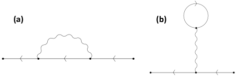
Before proceeding, we need to specify the free propagators of the spinful electrons and the phonons

$$\begin{split}G_{0}^{<}({\bm{k}},\omega)&=2\pi\mathrm{i}\sum_{a}|{\bm{k}}a\rangle\langle{\bm{k}}a|f_{{\bm{k}}a}\delta(\omega-\varepsilon_{{\bm{k}}a})\\ G_{0}^{\mathrm{r(a)}}({\bm{k}},\omega)&=\sum_{a}|{\bm{k}}a\rangle\langle{\bm{k}}a|\frac{1}{\omega-\varepsilon_{{\bm{k}}a}\pm\mathrm{i}\eta}\\ D_{0}^{<}({\bm{k}},\omega)&=-2\pi\mathrm{i}[(n_{{\bm{q}}}+1)\delta(\omega+\omega_{\bm{q}})+n_{{\bm{q}}}\delta(\omega-\omega_{\bm{q}})]\\ D_{0}^{\mathrm{r(a)}}({\bm{k}},\omega)&=\frac{1}{\omega-\omega_{{\bm{q}}}\pm\mathrm{i}\eta}-\frac{1}{\omega+\omega_{{\bm{q}}}\pm\mathrm{i}\eta},\end{split}$$ (S70)

where $f_{{\bm{k}}a}$ is the Fermi distribution for the electron in band basis $a=\pm$ and $n_{\bm{q}}$ is the phonon distribution. We now concretely evaluate Eq. (S69) with the shorthand ${\bm{k}}^{\prime}={\bm{k}}-{\bm{q}}$

$$\begin{split}\Sigma_{\mathrm{I}}^{<}({\bm{k}},\omega)&=\mathrm{i}\int\frac{\mathrm{d}\varepsilon}{2\pi}\sum_{\bm{q}}|g_{\bm{q}}|^{2}G_{0}^{<}({\bm{k}}^{\prime},\omega-\varepsilon)D_{0}^{<}({\bm{q}},\varepsilon)\\ &=2\pi\mathrm{i}\sum_{{\bm{q}}a}|g_{\bm{q}}|^{2}|{\bm{k}}^{\prime}a\rangle\langle{\bm{k}}^{\prime}a|f_{{\bm{k}}^{\prime}a}[(n_{{\bm{q}}}+1)\delta(\omega-\varepsilon_{{\bm{k}}^{\prime}a}+\omega_{\bm{q}})+n_{{\bm{q}}}\delta(\omega-\varepsilon_{{\bm{k}}^{\prime}a}-\omega_{\bm{q}})]\\ \Sigma_{\mathrm{I}}^{\mathrm{r}}({\bm{k}},\omega)&=\mathrm{i}\int\frac{\mathrm{d}\varepsilon}{2\pi}\sum_{\bm{q}}|g_{\bm{q}}|^{2}[G_{0}^{<}({\bm{k}}^{\prime},\omega-\varepsilon)D_{0}^{\mathrm{r}}({\bm{q}},\varepsilon)+G_{0}^{\mathrm{r}}({\bm{k}}^{\prime},\omega-\varepsilon)D_{0}^{<}({\bm{q}},\varepsilon)+G_{0}^{\mathrm{r}}({\bm{k}}^{\prime},\omega-\varepsilon)D_{0}^{\mathrm{r}}({\bm{q}},\varepsilon)]\\ &=\sum_{{\bm{q}}a}|g_{\bm{q}}|^{2}|{\bm{k}}^{\prime}a\rangle\langle{\bm{k}}^{\prime}a|\left[\frac{n_{\bm{q}}+1-f_{{\bm{k}}^{\prime}a}}{\omega-\varepsilon_{{\bm{k}}^{\prime}a}-\omega_{\bm{q}}+\mathrm{i}\eta}+\frac{n_{\bm{q}}+f_{{\bm{k}}^{\prime}a}}{\omega-\varepsilon_{{\bm{k}}^{\prime}a}+\omega_{\bm{q}}+\mathrm{i}\eta}\right]\\ \Sigma_{\mathrm{I}}^{\mathrm{a}}({\bm{k}},\omega)&={\Sigma_{\mathrm{I}}^{\mathrm{r}}}^{\dagger}({\bm{k}},\omega).\end{split}$$ (S71)

These expression can readily be used to calculate the lowest order correction Eq. (S66) in the electron Green’s function. For instance, we can look at the retarded $\Sigma_{\mathrm{I}}^{\mathrm{r}}$ in Eq. (S71). The process of absorption and emission of one phonon of momentum ${\bm{q}}$ manifests in the energy factors. Such inelastic scattering processes gives rise to the relaxation of the original spin-orbit coupled electronic state and hence the decoherence or a finite lifetime.

This formalism displays how one can take into account the interaction effects and consider the corresponding interaction-induced correction to the various single-particle electronic Green’s functions from the Keldysh-contour $G({\bm{k}},t_{1},t_{2})$ with spin degree of freedom, which are relevant to what SARPES measures experimentally. The characteristic relaxation times can be estimated from the quasiparticle lifetime embedded in the retarded self-energy. Because of the general matrix relation $(G^{\mathrm{r}})^{-1}=(G_{0}^{\mathrm{r}})^{-1}-\Sigma_{\mathrm{I}}^{\mathrm{r}}$, we switch the representation of $\Sigma_{\mathrm{I}}^{\mathrm{r}}$ to the eigenbasis $|{\bm{k}}a\rangle$ that diagonalizes $H_{0}={\bm{d}}({\bm{k}})\cdot{\bm{\sigma}}$ and hence $G_{0}^{\mathrm{r}}$. We therefore denote the unit vector $\hat{{\bm{d}}}$ in the diagonal basis and another unit vector $\hat{{\bm{d}}}^{\perp}$ normal to $\hat{{\bm{d}}}$ for the off-diagonal entries. We can make the following identification of the relaxation time scales respectively for the band-diagonal and band-offdiagonal contributions

$$\begin{split}T_{1}^{-1}\sim-2\mathrm{Im}\mathrm{Tr}[\hat{{\bm{d}}}\cdot{\bm{\sigma}}\Sigma_{\mathrm{I}}^{\mathrm{r}}]&=2\pi\sum_{{\bm{q}}a}K_{{\bm{q}}a}\left[(n_{\bm{q}}+1-f_{{\bm{k}}-{\bm{q}},a})\delta(\omega-\varepsilon_{{\bm{k}}-{\bm{q}},a}-\omega_{\bm{q}})+(n_{\bm{q}}+f_{{\bm{k}}-{\bm{q}},a})\delta(\omega-\varepsilon_{{\bm{k}}-{\bm{q}},a}+\omega_{\bm{q}})\right]\\ T_{2}^{-1}\sim-2\mathrm{Im}\mathrm{Tr}[\hat{{\bm{d}}}^{\perp}\cdot{\bm{\sigma}}\Sigma_{\mathrm{I}}^{\mathrm{r}}]&=2\pi\sum_{{\bm{q}}a}K^{\perp}_{{\bm{q}}a}\left[(n_{\bm{q}}+1-f_{{\bm{k}}-{\bm{q}},a})\delta(\omega-\varepsilon_{{\bm{k}}-{\bm{q}},a}-\omega_{\bm{q}})+(n_{\bm{q}}+f_{{\bm{k}}-{\bm{q}},a})\delta(\omega-\varepsilon_{{\bm{k}}-{\bm{q}},a}+\omega_{\bm{q}})\right],\end{split}$$ (S72)

where we denote $K_{{\bm{q}}a}=|g_{\bm{q}}|^{2}\mathrm{Tr}[\hat{{\bm{d}}}\cdot{\bm{\sigma}}|{\bm{k}}-{\bm{q}},a\rangle\langle{\bm{k}}-{\bm{q}},a|]$ and $K^{\perp}_{{\bm{q}}a}=|g_{\bm{q}}|^{2}\mathrm{Tr}[\hat{{\bm{d}}}^{\perp}\cdot{\bm{\sigma}}|{\bm{k}}-{\bm{q}},a\rangle\langle{\bm{k}}-{\bm{q}},a|]$. Note that these two scales are momentum- and frequency-dependent as per the Green’s function relation, where the physically relevant frequency is typically given by the band gap. Here we use the notation that $T_{1}$ is mainly for band energy relaxation and $T_{2}$ is for the interband decoherence time. Theoretically, as shown in Eq. (S72), because of the common origin from electron-phonon or electron-electron interaction, it is natural to expect that $T_{1}\sim T_{2}$ holds in general. Indeed, often a comparison in the range from $T_{2}\approx 0.5T_{1}$ to $T_{2}\lesssim 2T_{1}$ is observed in electronic spin experiments[8, 9]. For topological insulator surface state, usually $T_{1}$ is more accessible and estimated from spin-resolved spectroscopies to be at the order of $4\textrm{-}15\mathrm{ps}$[10, 6, 11]. This thus guarantees a coherence time $T_{2}$ at the same order, which is sufficient to observe the fine tornado patterns of our main interest, since these patterns rely on the interband quantum coherence. Also interestingly, from a quantum Boltzmann equation approach the topological insulator surface state is shown to have both the out-of-plane and in-plane spin relaxation times locked to twice the momentum relaxation time[12]. This can be regarded as an idealized yet still supporting evidence towards realistic detection of the physical information in the spin channel.

References

• Giannetti et al. [2016] C. Giannetti, M. Capone, D. Fausti, M. Fabrizio, F. Parmigiani, and D. Mihailovic, Ultrafast optical spectroscopy of strongly correlated materials and high-temperature superconductors: a non-equilibrium approach, Advances in Physics 65, 58 (2016).
• Nicoletti and Cavalleri [2016] D. Nicoletti and A. Cavalleri, Nonlinear light–matter interaction at terahertz frequencies, Advances in Optics and Photonics 8, 401 (2016).
• Smallwood et al. [2012] C. L. Smallwood, J. P. Hinton, C. Jozwiak, W. Zhang, J. D. Koralek, H. Eisaki, D.-H. Lee, J. Orenstein, and A. Lanzara, Tracking cooper pairs in a cuprate superconductor by ultrafast angle-resolved photoemission, Science 336, 1137 (2012).
• Gedik and Vishik [2017] N. Gedik and I. Vishik, Photoemission of quantum materials, Nat. Phys. 13, 1029 (2017).
• Sobota et al. [2021] J. A. Sobota, Y. He, and Z.-X. Shen, Angle-resolved photoemission studies of quantum materials, Reviews of Modern Physics 93, 025006 (2021).
• Loth et al. [2010] S. Loth, M. Etzkorn, C. P. Lutz, D. M. Eigler, and A. J. Heinrich, Measurement of fast electron spin relaxation times with atomic resolution, Science 329, 1628 (2010).
• Cocker et al. [2013] T. L. Cocker, V. Jelic, M. Gupta, S. J. Molesky, J. A. J. Burgess, G. D. L. Reyes, L. V. Titova, Y. Y. Tsui, M. R. Freeman, and F. A. Hegmann, An ultrafast terahertz scanning tunnelling microscope, Nature Photonics 7, 620 (2013).
• Eisele et al. [2014] M. Eisele, T. L. Cocker, M. A. Huber, M. Plankl, L. Viti, D. Ercolani, L. Sorba, M. S. Vitiello, and R. Huber, Ultrafast multi-terahertz nano-spectroscopy with sub-cycle temporal resolution, Nature Photonics 8, 841 (2014).
• Mitrano et al. [2016] M. Mitrano, A. Cantaluppi, D. Nicoletti, S. Kaiser, A. Perucchi, S. Lupi, P. D. Pietro, D. Pontiroli, M. Riccò, S. R. Clark, D. Jaksch, and A. Cavalleri, Possible light-induced superconductivity in K3C60 at high temperature, Nature 530, 461 (2016).
• Ostroverkhova [2016] O. Ostroverkhova, Organic optoelectronic materials: Mechanisms and applications, Chemical Reviews 116, 13279 (2016).
• Basov et al. [2017] D. N. Basov, R. D. Averitt, and D. Hsieh, Towards properties on demand in quantum materials, Nat. Mater. 16, 1077 (2017).
• Tokura et al. [2017] Y. Tokura, M. Kawasaki, and N. Nagaosa, Emergent functions of quantum materials, Nat. Phys. 13, 1056 (2017).
• Hasan and Kane [2010] M. Z. Hasan and C. L. Kane, Colloquium : Topological insulators, Rev. Mod. Phys. 82, 3045 (2010).
• Qi and Zhang [2011] X.-L. Qi and S.-C. Zhang, Topological insulators and superconductors, Rev. Mod. Phys. 83, 1057 (2011).
• Neupane et al. [2015] M. Neupane, S.-Y. Xu, Y. Ishida, S. Jia, B. M. Fregoso, C. Liu, I. Belopolski, G. Bian, N. Alidoust, T. Durakiewicz, V. Galitski, S. Shin, R. J. Cava, and M. Z. Hasan, Gigantic surface lifetime of an intrinsic topological insulator, Physical Review Letters 115, 116801 (2015).
• Chen et al. [2010] Y. L. Chen, J.-H. Chu, J. G. Analytis, Z. K. Liu, K. Igarashi, H.-H. Kuo, X. L. Qi, S. K. Mo, R. G. Moore, D. H. Lu, M. Hashimoto, T. Sasagawa, S. C. Zhang, I. R. Fisher, Z. Hussain, and Z. X. Shen, Massive Dirac fermion on the surface of a magnetically doped topological insulator, Science 329, 659 (2010).
• Chang et al. [2013] C.-Z. Chang, J. Zhang, X. Feng, J. Shen, Z. Zhang, M. Guo, K. Li, Y. Ou, P. Wei, L.-L. Wang, Z.-Q. Ji, Y. Feng, S. Ji, X. Chen, J. Jia, X. Dai, Z. Fang, S.-C. Zhang, K. He, Y. Wang, L. Lu, X.-C. Ma, and Q.-K. Xue, Experimental observation of the quantum anomalous hall effect in a magnetic topological insulator, Science 340, 167 (2013).
• Tokura et al. [2019] Y. Tokura, K. Yasuda, and A. Tsukazaki, Magnetic topological insulators, Nature Reviews Physics 1, 126 (2019).
• Wang et al. [2021] P. Wang, J. Ge, J. Li, Y. Liu, Y. Xu, and J. Wang, Intrinsic magnetic topological insulators, The Innovation 2, 100098 (2021).
• Kirilyuk et al. [2010] A. Kirilyuk, A. V. Kimel, and T. Rasing, Ultrafast optical manipulation of magnetic order, Reviews of Modern Physics 82, 2731 (2010).
• Kirilyuk et al. [2013] A. Kirilyuk, A. V. Kimel, and T. Rasing, Laser-induced magnetization dynamics and reversal in ferrimagnetic alloys, Reports on Progress in Physics 76, 026501 (2013).
• Hsieh et al. [2009] D. Hsieh, Y. Xia, D. Qian, L. Wray, J. H. Dil, F. Meier, J. Osterwalder, L. Patthey, J. G. Checkelsky, N. P. Ong, A. V. Fedorov, H. Lin, A. Bansil, D. Grauer, Y. S. Hor, R. J. Cava, and M. Z. Hasan, A tunable topological insulator in the spin helical Dirac transport regime, Nature 460, 1101 (2009).
• Xu et al. [2016] N. Xu, H. Ding, and M. Shi, Spin- and angle-resolved photoemission on the topological kondo insulator candidate: SmB6Journal of Physics: Condensed Matter 28, 363001 (2016).
• Wang et al. [2013] Y. H. Wang, H. Steinberg, P. Jarillo-Herrero, and N. Gedik, Observation of floquet-bloch states on the surface of a topological insulator, Science 342, 453 (2013).
• Oka and Kitamura [2019] T. Oka and S. Kitamura, Floquet engineering of quantum materials, Annual Review of Condensed Matter Physics 10, 387 (2019).
• Hosur [2011] P. Hosur, Circular photogalvanic effect on topological insulator surfaces: Berry-curvature-dependent response, Physical Review B 83, 035309 (2011).
• McIver et al. [2011] J. W. McIver, D. Hsieh, H. Steinberg, P. Jarillo-Herrero, and N. Gedik, Control over topological insulator photocurrents with light polarization, Nature Nanotechnology 7, 96 (2011).
• Reimann et al. [2018] J. Reimann, S. Schlauderer, C. P. Schmid, F. Langer, S. Baierl, K. A. Kokh, O. E. Tereshchenko, A. Kimura, C. Lange, J. Güdde, U. Höfer, and R. Huber, Subcycle observation of lightwave-driven Dirac currents in a topological surface band, Nature 562, 396 (2018).
• Yu et al. [2019] J. Yu, K. Zhu, X. Zeng, L. Chen, Y. Chen, Y. Liu, C. Yin, S. Cheng, Y. Lai, J. Huang, K. He, and Q. Xue, Helicity-dependent photocurrent of the top and bottom Dirac surface states of epitaxial thin films of three-dimensional topological insulators Sb2Te3Physical Review B 100, 235108 (2019).
• Schüler et al. [2020] M. Schüler, U. D. Giovannini, H. Hübener, A. Rubio, M. A. Sentef, and P. Werner, Local berry curvature signatures in dichroic angle-resolved photoelectron spectroscopy from two-dimensional materials, Science Advances 6, eaay2730 (2020).
• Cacho et al. [2015] C. Cacho, A. Crepaldi, M. Battiato, J. Braun, F. Cilento, M. Zacchigna, M. Richter, O. Heckmann, E. Springate, Y. Liu, S. Dhesi, H. Berger, P. Bugnon, K. Held, M. Grioni, H. Ebert, K. Hricovini, J. Minár, and F. Parmigiani, Momentum-resolved spin dynamics of bulk and surface excited states in the topological insulator Bi2Se3Physical Review Letters 114, 097401 (2015).
• Zhang et al. [2018] P. Zhang, K. Yaji, T. Hashimoto, Y. Ota, T. Kondo, K. Okazaki, Z. Wang, J. Wen, G. D. Gu, H. Ding, and S. Shin, Observation of topological superconductivity on the surface of an iron-based superconductor, Science 360, 182 (2018).
• Jozwiak et al. [2016] C. Jozwiak, J. A. Sobota, K. Gotlieb, A. F. Kemper, C. R. Rotundu, R. J. Birgeneau, Z. Hussain, D.-H. Lee, Z.-X. Shen, and A. Lanzara, Spin-polarized surface resonances accompanying topological surface state formation, Nature Communications 7, 13143 (2016).
• Nie et al. [2019] Z. Nie, I. C. E. Turcu, Y. Li, X. Zhang, L. He, J. Tu, Z. Ni, H. Xu, Y. Chen, X. Ruan, F. Frassetto, P. Miotti, N. Fabris, L. Poletto, J. Wu, Q. Lu, C. Liu, T. Kampen, Y. Zhai, W. Liu, C. Cacho, X. Wang, F. Wang, Y. Shi, R. Zhang, and Y. Xu, Spin-ARPES EUV beamline for ultrafast materials research and development, Applied Sciences 9, 370 (2019).
• Lv et al. [2019] B. Lv, T. Qian, and H. Ding, Angle-resolved photoemission spectroscopy and its application to topological materials, Nature Reviews Physics 1, 609 (2019).
• Fu [2009] L. Fu, Hexagonal warping effects in the surface states of the topological insulator Bi2Te3Physical Review Letters 103, 266801 (2009).
• Liu et al. [2010] C.-X. Liu, X.-L. Qi, H. Zhang, X. Dai, Z. Fang, and S.-C. Zhang, Model hamiltonian for topological insulators, Physical Review B 82, 045122 (2010).
• Cattelan and Fox [2018] M. Cattelan and N. Fox, A perspective on the application of spatially resolved ARPES for 2D materials, Nanomaterials 8, 284 (2018).
• Keatley et al. [2017] P. S. Keatley, T. H. J. Loughran, E. Hendry, W. L. Barnes, R. J. Hicken, J. R. Childress, and J. A. Katine, A platform for time-resolved scanning Kerr microscopy in the near-field, Review of Scientific Instruments 88, 123708 (2017).
• McCormick et al. [2017] E. J. McCormick, M. J. Newburger, Y. K. Luo, K. M. McCreary, S. Singh, I. B. Martin, E. J. Cichewicz, B. T. Jonker, and R. K. Kawakami, Imaging spin dynamics in monolayer WS2 by time-resolved Kerr rotation microscopy, 2D Materials 5, 011010 (2017).
• Yamamoto et al. [2018] S. Yamamoto, Y. Kubota, K. Yamamoto, Y. Takahashi, K. Maruyama, Y. Suzuki, R. Hobara, M. Fujisawa, D. Oshima, S. Owada, T. Togashi, K. Tono, M. Yabashi, Y. Hirata, S. Yamamoto, M. Kotsugi, H. Wadati, T. Kato, S. Iwata, S. Shin, and I. Matsuda, Femtosecond resonant magneto-optical Kerr effect measurement on an ultrathin magnetic film in a soft x-ray free electron laser, Japanese Journal of Applied Physics 57, 09TD02 (2018).
• Kamenev [2009] A. Kamenev, Field Theory of Non-Equilibrium Systems (Cambridge University Press, Cambridge, 2009).
• Stefanucci and van Leeuwen [2015] G. Stefanucci and R. van Leeuwen, Nonequilibrium Many-Body Theory of Quantum Systems (Cambridge University Press, New York, 2015).
• Freericks et al. [2009] J. K. Freericks, H. R. Krishnamurthy, and T. Pruschke, Theoretical description of time-resolved photoemission spectroscopy: Application to pump-probe experiments, Physical Review Letters 102, 136401 (2009).
• Kemper et al. [2018] A. Kemper, O. Abdurazakov, and J. Freericks, General principles for the nonequilibrium relaxation of populations in quantum materials, Physical Review X 8, 041009 (2018).
• Freericks et al. [2015] J. K. Freericks, H. R. Krishnamurthy, M. A. Sentef, and T. P. Devereaux, Gauge invariance in the theoretical description of time-resolved angle-resolved pump/probe photoemission spectroscopy, Physica Scripta T165, 014012 (2015).
• Freericks and Krishnamurthy [2016] J. Freericks and H. Krishnamurthy, Constant matrix element approximation to time-resolved angle-resolved photoemission spectroscopy, Photonics 3, 58 (2016).
• Xiao et al. [2010] D. Xiao, M.-C. Chang, and Q. Niu, Berry phase effects on electronic properties, Reviews of Modern Physics 82, 1959 (2010).
• Souza and Vanderbilt [2008] I. Souza and D. Vanderbilt, Dichroicf-sum rule and the orbital magnetization of crystals, Physical Review B 77, 054438 (2008).
• Yao et al. [2008] W. Yao, D. Xiao, and Q. Niu, Valley-dependent optoelectronics from inversion symmetry breaking, Physical Review B 77, 235406 (2008).
• Sheng et al. [2014] X.-L. Sheng, Z. Wang, R. Yu, H. Weng, Z. Fang, and X. Dai, Topological insulator to Dirac semimetal transition driven by sign change of spin-orbit coupling in thallium nitride, Physical Review B 90, 245308 (2014).
• Nie et al. [2017] S. Nie, G. Xu, F. B. Prinz, and S.-C. Zhang, Topological semimetal in honeycomb lattice LnSI, Proceedings of the National Academy of Sciences 114, 10596 (2017).
• Iyer et al. [2018] V. Iyer, Y. Chen, and X. Xu, Ultrafast surface state spin-carrier dynamics in the topological insulator Bi2Te2Se, Physical Review Letters 121, 026807 (2018).
• Press et al. [2007] W. H. Press, S. A. Teukolsky, W. T. Vetterling, and B. P. Flannery, Numerical Recipes: The Art of Scientific Computing, 3rd ed. (Cambridge University Press, Cambridge, 2007).
• Bar-Gill et al. [2013] N. Bar-Gill, L. Pham, A. Jarmola, D. Budker, and R. Walsworth, Solid-state electronic spin coherence time approaching one second, Nature Communications 4, 1743 (2013).
• Sigillito et al. [2015] A. Sigillito, R. Jock, A. Tyryshkin, J. Beeman, E. Haller, K. Itoh, and S. Lyon, Electron spin coherence of shallow donors in natural and isotopically enriched germanium, Physical Review Letters 115, 247601 (2015).
• Liu and Sinova [2013] X. Liu and J. Sinova, Reading charge transport from the spin dynamics on the surface of a topological insulator, Physical Review Letters 111, 166801 (2013).