Global convergence and asymptotic optimality of the heavy ball method for a class of non-convex optimization problems

Abstract

In this letter we revisit the famous heavy ball method and study its global convergence for a class of non-convex problems with sector-bounded gradient. We characterize the parameters that render the method globally convergent and yield the best $R$-convergence factor. We show that for this family of functions, this convergence factor is superior to the factor obtained from the triple momentum method.

I Introduction

We consider the optimization problem

$$\min_{x\in\mathbf{R}^{n}}f(x)$$ (1)

along with the well-known heavy ball (HB) method

$$x_{t+1}=x_{t}-\alpha\nabla f(x_{t})+\beta(x_{t}-x_{t-1}),\quad{t=0,1,\ldots,}$$ (2)

where $f:\mathbf{R}^{n}\to\mathbf{R}$ is differentiable and potentially non-convex and $\nabla f(x)$ denotes the gradient of $f(x)$. The parameters $\alpha$ and $\beta$ are positive scalar constants. Convergence properties of such iterative processes have been widely studied; e.g., see [11, 13, 10]. It is also recognized that iterative processes of the form (2) can be analyzed using tools from robust control theory [7, 8, 14, 16], since equation (2) can be written in the form of a nonlinear dynamic system of Luré type.

The original local convergence properties of (2) as well as optimal choices for $\alpha$ and $\beta$ that yield the fastest $R$-convergence properties, see [11], were presented in [13]. We refer to these optimal parameters as Polyak’s parameters for the rest of this paper. Since then many researchers have contemplated the question of the global convergence of (2). For example, as stated in [7] for a certain family of strongly convex cost functions with Lipschitz gradient, the system (2) with Polyak’s parameters may not be globally convergent. In [3], intervals for the algorithm parameters are introduced that render (2) globally convergent. However, that work does not focus on the relationship between the method’s parameters and its convergence rate. More recently, a globally convergent first order optimization algorithm, the triple momentum method (TMM), for solving optimization problems with strongly convex cost function whose gradient is Lipschitz is introduced in [16]. It is further shown that one can choose the parameters for this algorithm to obtain the best hitherto convergence property among all globally convergent methods.

In this paper, we consider a more general class of functions compared to the aforementioned results. Specifically, inspired by the observations in [9], we consider optimization problems with unimodal objective functions which may not be globally convex, and are only convex in the infinitesimally small region in the vicinity of the minimum $x^{*}$. Specifically, we consider the problems whose cost functions satisfy the following assumption.

Assumption 1

There exists a point $x^{*}$ such that the minimum of $f(x)$ is attained at $x^{*}$. Moreover, there exist constants $m$, $L$, $(L\geq m>0)$, such that for every $x\in\mathbf{R}^{n}$,

$$\left(m(x-x^{*})-\nabla f(x)\right)^{T}\left(L(x-x^{*})-\nabla f(x)\right)\leq 0.$$ (3)

The class of objective functions with this property will be denoted $\mathscr{F}_{m,L}^{1}$.

An example of a function in $\mathscr{F}_{m,L}^{1}$ is depicted in Fig. 1.

We specifically employ the circle criterion for absolute stability of discrete time Luré systems with sector-bounded nonlinearities to derive expressions for the parameters of the heavy ball method (2) that guarantee its global convergence and optimize its $R$-convergence factor. To distinguish this choice of parameters from Polyak’s parameters [13], we name them generalized heavy ball (GHB) parameters. Moreover, we investigate the global convergence of the triple momentum method for non-convex functions using the circle criterion. Specifically, for a given Lipschitz constant $L$, we derive a bound on the size of the sector, in terms of the ratio $L/m$, such that TMM can be guaranteed to be globally converging for all functions of class $\mathscr{F}_{m,L}^{1}$. We also identify the cases where (2) with GHB parameters enjoys a better $R$-convergence property compared to TMM.

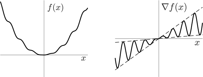
Figure 1: A non-convex objective function $f(x)\in\mathscr{F}_{m,L}^{1}$ where $f(x)=\frac{L-m}{4}\left(\frac{L+m}{L-m}x^{2}+\frac{2}{\omega^{2}}\sin(\omega x)-\frac{2}{\omega}x\cos(\omega x)\right)$, with positive scalars $L$, $m$, and $\omega$ such that $L>m$.

II Background

Before continuing further we briefly discuss the family of functions that satisfy Assumption 1. Condition (3) is known as the sector condition in the absolute stability theory [6]. This terminology owes to the graphical interpretation of the inequality (3) in the case $x\in\mathbf{R}$ where (3) implies that the graph of the derivative $f^{\prime}(x)$ is enclosed in the sector formed by the lines $m(x-x^{*})$ and $L(x-x^{*})$; see Fig. 1. It is worth to compare Assumption 1 with other assumptions on the objective function $f(x)$ that appear in the literature. First, since $f(x)$ attains its minimum at $x^{*}$, then $\nabla f(x^{*})=0$. When the function $f$ is two times differentiable, this allows us to conclude from (3) that the Hessian of $f$ at $x^{*}$, denoted $\Delta=\nabla^{2}f(x^{*})$, satisfies the often-quoted condition (e.g., see [13, Theorem 1, p.65])

$$mI\leq\Delta\leq LI.$$ (4)

We denote the class of such objective functions $\mathscr{F}_{m,L}^{2}$.

The second connection is with the class $\mathscr{S}_{m_{0},L_{0}}^{1,1}$ of continuously differentiable strongly convex functions $f:\mathbf{R}^{n}\to\mathbf{R}$ with Lipschitz continuous gradient [7, 14, 8] such that for all $x,y\in\mathbf{R}^{n}$

$$m_{0}\|x-y\|^{2}\leq(\nabla f(x)-\nabla f(y))^{T}(x-y)\leq L_{0}\|x-y\|^{2}.$$ (5)

It is shown in [7, Proposition 5] that any $f\in\mathscr{S}_{m_{0},L_{0}}^{1,1}$ satisfies the sector condition (3) with $m=m_{0}$, $L=L_{0}$, i.e., $\mathscr{S}_{m_{0},L_{0}}^{1,1}\subset\mathscr{F}_{m,L}^{1}$ when $m=m_{0}$, $L=L_{0}$. In this case, $m$ characterizes the coercivity property of the convex function $f$ while $L$ is the Lipschitz constant of $\nabla f$. Of course, Assumption 1 describes a larger class of objective functions than the class of convex functions captured by (5). It includes functions which are not convex (see Fig. 1). It follows from (3) that every sector-bounded $f$ is an invex function [1]. When $x\in\mathbf{R}$, every such function is pseudoconvex.

For a strongly convex function $f\in\mathscr{S}_{m,L}^{1,1}$, $\kappa=L/m$ is known as the condition number, but for functions $f\in\mathscr{F}_{m,L}^{1}$, it characterizes the relative ‘width’ of the sector containing $\nabla f$. This ratio will help us to compare our results with those obtained in the literature for strongly convex functions.

II-A Heavy ball method as Luré feedback control systems

As pointed out in [7, 8, 14], the iterative process (2) can be written in the form of a nonlinear dynamic system

$$X_{t+1}=AX_{t}+BU_{t},$$ (6)

$$Y_{t}=CX_{t},\quad U_{t}=-\phi(Y_{t}),$$

whose state, output and nonlinearity are respectively $X_{t}=\begin{bmatrix}x_{t-1}^{T}&x_{t}^{T}\end{bmatrix}^{T}$, $\phi(Y_{t})=\nabla f(Y_{t}).$ The matrices $A\in\mathbf{R}^{2n\times 2n}$, $B\in\mathbf{R}^{2n\times n}$, and $C\in\mathbf{R}^{n\times 2n}$ are defined as $A=A_{0}\otimes I_{n},\quad B=B_{0}\otimes I_{n},\quad C=C_{0}\otimes I_{n}$ with

$$A_{0}=\begin{bmatrix}0&\quad 1\\ -\beta&\quad 1+\beta\end{bmatrix},\quad B_{0}=\begin{bmatrix}0\\ \alpha\end{bmatrix},\quad C_{0}=\begin{bmatrix}0&\quad 1\end{bmatrix}.$$

Similarly, $X^{*}=\begin{bmatrix}1&~{}1\end{bmatrix}^{T}\otimes x^{*}$ is the unique equilibrium of (6). We refer the reader to [7] for a detailed introduction to analysis and design of iterative optimization algorithms using tools from robust control theory.

The system (6) is the feedback control system of Luré type [5, 6]. There are a number of results in the literature concerned with stability of Luré systems. In this note we will make use of the multivariate version of the so-called Tsypkin’s circle criterion [5] to obtain sufficient conditions for global asymptotic convergence of the Luré systems of the form (6) subject to the sector condition (3); also see [4]. Admittedly, the circle criterion is the simplest and the least accurate in terms of capturing properties of the function $f$. However, it proves to be sufficient for the purpose of this letter which is to demonstrate the applicability of the heavy ball method beyond the class of strongly convex objectives.

II-B $R$-convergence

Here we recall some basic definitions which formalize the notion of the rate of convergence of an iterative process.

Definition 1 ([11],p.288)

Let $\{x_{t}\}$ be a sequence that converges to $x^{*}$. Then the number $r_{\{x_{t}\}}=\limsup_{t\to\infty}\|x_{t}-x^{*}\|^{1/t}$ is the root-convergence factor, or $R$-factor of $\{x_{t}\}$. If $\mathscr{I}$ is an iterative process with limit point $x^{*}$, and $\mathfrak{C}(\mathscr{I},x^{*})$ is the set of all sequences generated by $\mathscr{I}$ which converge to $x^{*}$, then $r_{\mathscr{I}}=\sup\{r_{\{x_{t}\}}:\{x_{t}\}\in\mathfrak{C}(\mathscr{I},x^{*})\}$ is the $R$-factor of $\mathscr{I}$ at $x^{*}$.

Remark 1

The $R$-factor characterizes an asymptotic convergence rate of $\{x_{t}\}$.

Definition 2

Let $x_{t}$ denote the vector of iterates of the algorithm (2) at step $t$ initiated at time $0$ with $x_{0},x_{-1}$. The algorithm is said to converge globally asymptotically to $x^{*}$ if its iterates have the following properties:

1. for every $\epsilon>0$ there exists $\delta=\delta(\epsilon)>0$ such that $\|x_{-1}-x^{*}\|<\delta$, $\|x_{0}-x^{*}\|<\delta$ imply that $\|x_{t}-x^{*}\|<\epsilon$ for all $t\geq 0$; and

2. $\lim_{t\to\infty}\|x_{t}-x^{*}\|=0$ uniformly in $x_{0}$, $x_{-1}$ for all $x_{0},x_{-1}\in\mathbf{R}^{n}$.

III Global convergence analysis

In this section we analyze two optimization methods (2), the heavy ball method due to Polyak [12, 13] and the triple momentum method of [16] when applied to non-convex objective functions from class $\mathscr{F}_{m,L}^{1}$ and are initiated arbitrarily far from $x^{*}$. Both methods are two-step first order ‘accelerated gradient’ methods, manifesting excellent convergence properties. The heavy ball method with Polyak’s parameters achieves the smallest $R$-factor when it is initiated sufficiently close to $x^{*}$ and $f\in\mathscr{F}_{m,L}^{2}$ [13]. Hence, it is the ‘asymptotically fastest’ method.

Our analysis employs the circle criterion for absolute stability of general discrete-time time-varying Luré systems with sector-bounded nonlinearity given in [5, p.841]. We present it in the form specialized for the setting of the algorithm (2) and Luré system (6) with a nonzero point of attraction. Let $Q(z)$ be the transfer function of the linear part of the Luré system (6). Then $Q(z)=Q_{0}(z)\otimes I_{n}$, where

$$Q_{0}(z)\sim\left[\begin{array}[]{c|c}A_{0}&B_{0}\\ \hline\cr C_{0}&0\end{array}\right].$$ (7)

Lemma 1 (Circle criterion, [5], p.841)

Suppose that the transfer function

$$H(z)=[1+LQ_{0}(z)][1+mQ_{0}(z)]^{-1}\otimes I_{n}$$ (8)

is strict positive real. Then for any function $f\in\mathscr{F}_{m,L}^{1}$, the algorithm (2) globally asymptotically converges to $x^{*}$.

III-A Global convergence of (2) with Polyak’s parameters

It is well known [12, 13] that when $f\in\mathscr{F}_{m,L}^{2}$ and

$$0\leq\beta<1,\quad 0<\alpha<2(1+\beta)L^{-1},$$ (9)

one can find an $\epsilon>0$ such that for any $x_{0}$, $x_{-1}$ such that $\|x_{-1}-x^{*}\|\leq\epsilon$, $\|x_{0}-x^{*}\|\leq\epsilon$, the sequence of iterates $x_{t}$ generated by (2) converges to $x^{*}$ exponentially fast, $\|x_{t}-x^{*}\|\leq c(\delta)(\rho+\delta)^{t}$, where $0\leq\rho<1$, $0<\delta<1-\rho$. Under these conditions, the minimal $\rho$ is achieved when

$$\alpha=\alpha_{\mathrm{P}}\triangleq\frac{4}{(\sqrt{L}+\sqrt{m})^{2}},\quad\beta=\beta_{\mathrm{P}}\triangleq\frac{(\sqrt{L}-\sqrt{m})^{2}}{(\sqrt{L}+\sqrt{m})^{2}}$$ (10)

and is equal to

$$r_{\mathrm{P}}\triangleq\frac{\sqrt{L}-\sqrt{m}}{\sqrt{L}+\sqrt{m}}.$$ (11)

The parameters $\alpha_{\mathrm{P}}$ and $\beta_{\mathrm{P}}$ are the Polyak’s parameters discussed in the introduction.

According to [7], for a strongly convex function $f$ subject to the sector condition (3), convergence of the heavy ball algorithm (2), (10) can be guaranteed when $\kappa=L/m$ is approximately equal to $6$ or less. This threshold is calculated numerically [7] and represents a point where the LMIs used to characterize the global stability of (2) fail to be satisfied. The next theorem gives a precise meaning to this observation. It derives a range of ratios $L/m$ ($L$, $m$ are the sector bound constants from (3)) for which the heavy ball algorithm (2) with Polyak’s parameters converges globally for all functions of class $\mathscr{F}_{m,L}^{1}$ in the sense of Definition 2.

Theorem 1

If

$$L/m<\kappa_{0}\triangleq 3+2\sqrt{2},$$ (12)

then the heavy ball method (2), (10) globally asymptotically converges to $x^{*}$ for any $f\in\mathscr{F}_{m,L}^{1}$.

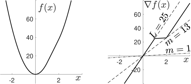
Figure 2: The function $f(x)$ in Example 1.

Remark 2

The threshold $\kappa_{0}=3+2\sqrt{2}$ on the ratio $L/m$ stated in Theorem 1 is close to the approximate threshold of 6 obtained in [7] using numerical search. This is not surprising as the circle criterion is the approach that underpins the stability analysis of [7] in deriving this threshold. $\blacksquare$

Proof of Theorem 1: With $\alpha$ and $\beta$ given in (10), the transfer function $H(z)$ in equation (8) becomes $H(z)=\left(\frac{z+\beta^{1/2}}{z-\beta^{1/2}}\right)^{2}I_{n}$. According to Lemma 1, to establish the claim of the theorem it suffices to show that if $L/m<\kappa_{0}=3+2\sqrt{2}$, then $H(z)$ is strictly positive real. This requires us to show that $\left|\arg\left(\frac{e^{j\omega}+\beta^{1/2}}{e^{j\omega}-\beta^{1/2}}\right)\right|<\frac{\pi}{4}$ for all $\omega\in[-\pi,\pi]$. Equivalently, it suffices to show that

$$\min_{\omega\in[-\pi,\pi]}\cos\left(\arg\left(\frac{e^{j\omega}+\beta^{1/2}}{e^{j\omega}-\beta^{1/2}}\right)\right)>\frac{1}{\sqrt{2}}.$$ (13)

However, $\min_{\omega\in[-\pi,\pi]}\cos\left(\arg\left(\frac{e^{j\omega}+\beta^{1/2}}{e^{j\omega}-\beta^{1/2}}\right)\right)=\frac{1-\beta}{1+\beta}$. Using the definition of $\beta$ in (10), it is straightforward to verify that $\frac{1-\beta}{1+\beta}>\frac{1}{\sqrt{2}}$ and $H(z)$ is strictly positive real if and only if $L/m<\kappa_{0}$. Thus, the conditions of the circle criterion in Lemma 1 are satisfied under condition (12), and the statement of the theorem follows from Lemma 1. $\Box$

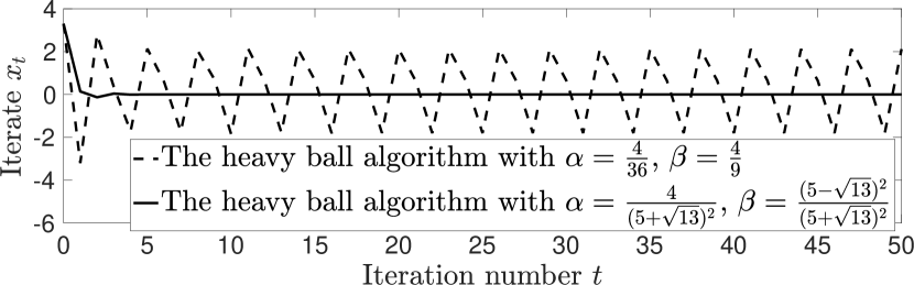
Figure 3: The trajectories of the two versions of the heavy ball algorithm for the function in Example 1.

Example 1

Reference [7] gives an example of a strongly convex function $f(x)$ of one-dimensional variable $x$ that leads to a non-convergent heavy ball method (see Fig. 2):

$$f(x)=\begin{cases}\frac{25}{2}x^{2},&x<1,\\ \frac{1}{2}x^{2}+24x-12,&1\leq x<2,\\ \frac{25}{2}x^{2}-24x+36,&x\geq 2,\end{cases}$$ (14)

The function has minimum at $x^{*}=0$. It satisfies (5) with $m_{0}=1$, $L_{0}=25$, which implies that it also satisfies the sector condition (3) with $m=1$, $L=25$. It was observed in [7] that using these values of $m$ and $L$ in (10) to define the Polyak’s parameters leads to an algorithm which, when initiated within a certain range of initial conditions, converges to a limit cycle, instead of the minimum point $x^{*}=0$. The values of $\alpha$ and $\beta$ for which this behavior was observed were $\alpha=\frac{4}{36}$, $\beta=\frac{4}{9}$.

However, from Fig. 2 one can see readily that the function $f(x)$ in this example also satisfies the sector condition (3) with $m=13$, $L=25$. These values of $m$, $L$ render the condition (12) of Theorem 1 true, thus the heavy ball algorithm (2) with Polyak’s parameters $\alpha=\frac{4}{(5+\sqrt{13})^{2}}$, $\beta=\frac{(5-\sqrt{13})^{2}}{(5+\sqrt{13})^{2}}$ obtained using $m=13$, $L=25$ must globally asymptotically converge to $x^{*}=0$. Fig. 3 confirms this. Both trajectories in this figure are initiated with the same initial condition $x_{-1}=x_{0}=3.3$.

This example highlights the importance of deciding what values $m$ and $L$ are to be used for tuning the heavy ball method. The values of $m$ and $L$ such that the condition (5) is satisfied may be conservative for tuning the heavy ball algorithm, even for convex functions. However, using values of $m$ and $L$ such that the sector condition (3) is satisfied, may be less conservative. This is not surprising since these conditions are not equivalent: (5) implies (3) but not vice versa. Thus, one should exercise caution when quoting this example as a counter-example for global convergence of (2).

III-B Global convergence of TMM

The triple momentum method [16] is given by

$$x_{t+1} =(1+\beta)x_{t}-\beta x_{t-1}-\alpha\nabla f(y_{t}),$$

$$y_{t} =(1+\gamma)x_{t}-\gamma x_{t-1},$$

$$\eta_{t} =(1+\delta)x_{t}-\delta x_{t-1}.$$ (15)

The coefficients $\alpha$, $\beta$, $\gamma$ and $\delta$ were defined in [16] as

$$(\alpha,\beta,\gamma,\delta)=\left(\frac{1+\rho}{L},\frac{\rho^{2}}{2-\rho},\frac{\rho^{2}}{(1+\rho)(2-\rho)},\frac{\rho^{2}}{1-\rho^{2}}\right),$$ (16)

where $\rho=1-\sqrt{\kappa^{-1}}$, $\kappa$ is the condition number of a strongly convex function, and $L$ is the Lipschitz constant of its gradient; see (5). As noted, any such function belongs to the class $\mathscr{F}_{m,L}^{1}$ with $m=L/\kappa$. The process (III-B) can be represented as a Luré system of the form (6) with the state $X_{t}=[x_{t-1}^{T}~{}x_{t}^{T}]^{T}$, the output $Y_{t}=[-\gamma I_{n}~{}(1+\gamma)~{}I_{n}]X_{t}$ and the additional performance output $\eta_{t}=[-\delta I_{n}~{}(1+\delta)~{}I_{n}]X_{t}$ which is not fed back into (6). Therefore global asymptotic convergence of this method can be analyzed using the circle criterion, and the assumption of strong convexity of $f$ can be relaxed to $f\in\mathscr{F}_{m,L}^{1}$, where $m=L/\kappa$, and $\kappa>0$ can be regarded as a given constant.

Consider the polynomial $\chi(\rho)=8-\rho-8\rho^{2}-14\rho^{3}-\rho^{5}.$ This polynomial is monotone decreasing in $\rho$ when $\rho>0$, and it has the unique real root $\rho_{0}\approx 0.650307$. Define $\kappa_{\mathrm{TM}}\triangleq(1-\rho_{0})^{-2}\approx 8.1776.$

Theorem 2

Let $\kappa$ be a positive constant, and $f$ be an arbitrary function in $\mathscr{F}_{m,L}^{1}$, where $m=L/\kappa$. If $\kappa<\kappa_{\mathrm{TM}}$, then each sequence of iterates $x_{t}$, $y_{t}$ and $\eta_{t}$ generated by (III-B) globally asymptotically converges to $x^{*}$.

Proof: With $\alpha$, $\beta$, $\gamma$ and $\delta$ defined in (16), the transfer function $H(z)$ defined in Lemma 1 is $H(z)=\frac{z(\rho+z)}{(z-\rho)\left(z-\rho^{2}\right)}I.$ We now show that $H(z)$ is strict positive real for $\kappa<\kappa_{\mathrm{TM}}$. For this, it suffices to show that for all $\omega\in[-\pi,\pi]$,

$$\psi(\omega) \triangleq \mathrm{Re}\left[e^{j\omega}(\rho+e^{j\omega})(e^{-j\omega}-\rho)(e^{-j\omega}-\rho^{2})\right]$$ (17)

$$= \rho^{4}\cos\omega-2\rho^{3}\sin^{2}\omega-\rho^{2}\cos\omega-\rho^{2}+1>0.\qquad$$

When $\rho\in(0,\sqrt{5}-2)$, the function $\psi(\omega)$ has minimum at $\omega=0$, and $\psi(0)=(1-\rho^{2})^{2}>0$ for any $\rho$ in this interval.

When $\rho\in[\sqrt{5}-2,1)$, the function $\psi(\omega)$ has two minimums at $\omega=\pm\cos^{-1}\left(\frac{1-\rho^{2}}{4\rho}\right)$. The function is even, therefore it has the same value of $\frac{1}{8}\chi(\rho)$ at those points. Since $\chi(\rho)$ is monotone decreasing and $\chi(\rho)\leq 0$ for $\rho\geq\rho_{0}$, we conclude that $H(z)$ is strict positive real in this case if and only if $\rho<\rho_{0}$.

Combining these two cases, we note that the conditions of Lemma 1 are satisfied when $\kappa<\kappa_{\mathrm{TM}}$, and the claim of the theorem follows from that lemma. $\Box$

Theorem 2 shows that TMM tuned for a strongly convex function $f\in\mathscr{S}_{m_{0},L}^{1,1}$ with the condition number $\kappa<\kappa_{\mathrm{TM}}$ remains globally converging for non-convex functions of the class $\mathscr{F}_{m,L}^{1}$ with $m=m_{0}=L/\kappa$.

IV Global convergence of the heavy ball method with GHB parameters and the corresponding $R$-convergence factor

Example 1 motivates us to address the question raised in [7] as to whether the heavy ball method converges globally over the class of functions captured by the sector condition (3) for some choice of $\alpha$ and $\beta$ than other the Polyak’s parameters (10). Using the circle criterion allows us to answer this question, without making a priori assumptions about the ratio $\kappa=L/m$.

Introduce the function

$$\bar{\alpha}(\beta)=\begin{cases}2(1+\beta)L^{-1},&\beta\leq\left(\sqrt{\frac{L}{m}}-\sqrt{\frac{L}{m}-1}\right)^{2},\\ \frac{2(1-\beta)^{2}}{(1+\beta)(L+m)-4\sqrt{\beta Lm}},&\beta>\left(\sqrt{\frac{L}{m}}-\sqrt{\frac{L}{m}-1}\right)^{2};\end{cases}$$ (18)

Theorem 3

For any $L$, $m$ such that $L>m>0$, if

$$0\leq\beta<1,\quad 0<\alpha<\bar{\alpha}(\beta),$$ (19)

then the algorithm (2) globally asymptotically converges to $x^{*}$ for all functions $f\in\mathscr{F}_{m,L}^{1}$.

$$\beta_{0}(\kappa)=\frac{\kappa\left(\kappa\left(-\sqrt{2}\sqrt{\frac{(\kappa-1)\left(\left(\sqrt{\frac{\kappa-8}{\kappa}}+1\right)\kappa^{2}+\left(7\sqrt{\frac{\kappa-8}{\kappa}}-5\right)\kappa+12\right)}{\kappa^{3}}}+\sqrt{\frac{\kappa-8}{\kappa}}+1\right)-\sqrt{\frac{\kappa-8}{\kappa}}+7\right)^{2}}{16(\kappa+1)^{2}}$$ (20)

Proof: According to Lemma 1, it suffices to show that

$$H(z)=\frac{z^{2}+\left(L\alpha-1-\beta\right)z+\beta}{z^{2}+\left(m\alpha-1-\beta\right)z+\beta}I_{n}$$ (21)

is strictly positive real when $\alpha$, $\beta$ satisfy (19). For this, we use the criterion for strict positive realness due to Šiljak; see [15, Theorem 2].

Let $p(z)$, $q(z)$ denote the denominator and the numerator of $H(z)$. Since $\bar{\alpha}(\beta)<2(1+\beta)L^{-1}$ in the interval $\beta\in\left(\left(\sqrt{L/m}-\sqrt{L/m-1}\right)^{2},1\right]$, one can use the Jury criterion to confirm that the polynomial

$$\frac{1}{2}(p(z)+q(z))=z^{2}+\left(\frac{m+L}{2}\alpha-1-\beta\right)z+\beta$$ (22)

is Schur stable under conditions (19). This validates condition (i) of Theorem 2 in [15].

Condition (ii) of that theorem requires that the polynomial $g(z)=\frac{1}{2}z^{2}(p(z)q(z^{-1})+p(z^{-1})q(z))$ must have exactly two roots inside and two roots outside the unit circle. To validate this requirement, we note that $g(z)$ is a self-inversive polynomial, hence it can be written as $g(z)=b_{2}z^{4}+b_{1}z^{3}+2b_{0}z^{2}+b_{1}z+b_{2}$. We now use the modified Schur-Cohn-Marden method for enumerating the zeros of a self-inversive polynomial within the unit circle [2]. According to this method, $g(z)$ has exactly two zeros inside and two zeros outside the unit disk if and only if $b_{1}^{2}-\left(b_{0}+b_{2}\right)^{2}<0$ and either $16b_{2}^{2}-b_{1}^{2}<0$, or $16b_{2}^{2}-b_{1}^{2}>0$ and $\left(16b_{0}b_{2}-3b_{1}^{2}\right)^{2}>\left(16b_{2}^{2}-b_{1}^{2}\right)^{2}.$ The analysis of these conditions shows that they are equivalent to condition (19). $\Box$

Remark 3

When $\beta\leq\left(\sqrt{L/m}-\sqrt{L/m-1}\right)^{2}$, the upper bound on $\alpha$ in (19) is the same as that given in Polyak’s theorem on stability of the heavy ball method [13, Theorem 1, p.65]; see (9). Therefore, for this range of the inertia parameter $\beta$, Theorem 3 complements Polyak’s theorem by showing that the heavy ball method converges globally. When $\beta>\left(\sqrt{L/m}-\sqrt{L/m-1}\right)^{2}$, Theorem 3 guarantees global convergence only when the stepsize parameter $\alpha$ is less than $\bar{\alpha}(\beta)$, i.e., in the smaller range of $\alpha$ than that established by Polyak’s theorem. $\blacksquare$

Remark 4

In [3], it is shown that for a strongly convex Lipschitz-continuous $f$, if $\beta\in(0,1)$ and $\alpha\in\left(0,\frac{2(1-\beta)}{L+m}\right),$ then (2) converges with an $R$-factor less than 1. We now compare this result with Theorem 3. It is easy to see that $\frac{2(1-\beta)}{L+m}<2(1+\beta)L^{-1}$. Also, when $\left(\sqrt{\frac{L}{m}}-\sqrt{\frac{L}{m}-1}\right)^{2}<\beta\leq\frac{4Lm}{(L+m)^{2}}$, then $\bar{\alpha}(\beta)\geq\frac{2(1-\beta)}{L+m}$. When $\beta\in(\frac{4Lm}{(L+m)^{2}},1)$, the opposite inequality holds. These inequalities allow us to compare the conditions in [3] with the result of Theorem 3 and condition (19) of that theorem. We conclude that for $\beta\in(0,\frac{4Lm}{(L+m)^{2}})$, our result provides a wider range of $\alpha$ under which the GHB method is globally convergent. This conclusion holds even when $f$ is not strongly convex. $\blacksquare$

Next, we derive an upper bound on the optimal $R$-factor of the globally converging algorithm (2) for the parameter choice of Theorem 3, which we denote $r_{\mathrm{GHB}}$. This will be achieved by optimizing the $R$-factor of the iterative process (2) over the parameter region defined by the global convergence condition (19). To derive such a bound, we restrict attention to objective functions $f\in\mathscr{F}_{m,L}^{2}$.

To present this result, some notation is needed. Let $\rho(A(\Delta))$ denote the spectral radius of the matrix

$$A(\Delta)=\left[\begin{array}[]{cc}0&I\\ -\beta I{}&~{}(1+\beta)I-\alpha\Delta\end{array}\right],\quad\Delta=\nabla^{2}f(x^{*}).$$ (23)

Also, introduce $\gamma_{m}=\gamma_{m}(\alpha,\beta)=m\alpha-1-\beta$, and $\gamma_{L}=\gamma_{L}(\alpha,\beta)=L\alpha-1-\beta$. It can be shown that for every $\kappa=L/m>8$ the function $\eta(\beta)\triangleq\frac{-\gamma_{m}(\bar{\alpha}(\beta),\beta)+\sqrt{\gamma_{m}(\bar{\alpha}(\beta),\beta)^{2}-4\beta}}{2}$ has a unique local minimum in the interval $\beta\in((\sqrt{\kappa}-\sqrt{\kappa-1})^{2},1)$. This minimum is attained at $\beta=\beta_{0}(\kappa)$ defined in equation (20) shown at the top of the page. Next, let us define $\nu(\kappa)\triangleq\frac{2-\sqrt{2\sqrt{\kappa}+3-\kappa}}{\sqrt{\kappa}-1}$. This quantity is well defined in the interval $\kappa\in[\kappa_{0},9]$ where $\kappa_{0}$ is the constant defined in (12). Finally, it can be shown that in the interval $\kappa\in[8,9]$ the equation $\eta(\beta_{0}(\kappa))=\nu(\kappa)$ has a unique solution $\bar{\kappa}\approx 8.2975$.

Theorem 4

Let $\mathscr{A}_{\mathrm{GHB},m,L}$ denote the set of all pairs $(\alpha,\beta)$ for which the algorithm (2) converges globally for all $f\in\mathscr{F}_{m,L}^{2}$. Then $\inf_{\mathscr{A}_{\mathrm{GHB},m,L}}\sup_{\mathscr{F}_{m,L}^{2}}r_{\mathrm{GHB}}\leq r^{*}$, where the constant $r^{*}$ is defined by

$$r^{*}=\min\{\sup_{\Delta}\rho(A(\Delta)):\alpha\in(0,\bar{\alpha}(\beta)),\beta\in[0,1)\}.$$ (24)

The supremum in (24) is over the set of matrices $\Delta$ which satisfy (4). The constant $r^{*}$ has the following value

$$r^{*}=\begin{cases}\frac{\sqrt{L}-\sqrt{m}}{\sqrt{L}+\sqrt{m}},&1<\frac{L}{m}\leq\kappa_{0},\\ \nu(L/m)&\kappa_{0}\leq\frac{L}{m}<\bar{\kappa},\\ \eta(\beta_{0}(L/m)),&\frac{L}{m}\geq\bar{\kappa}.\end{cases}$$ (25)

The minimum in (24) is achieved when

$$\alpha=\alpha^{*}\triangleq\begin{cases}\frac{4}{(\sqrt{L}+\sqrt{m})^{2}},&1<\frac{L}{m}\leq\kappa_{0},\\ \bar{\alpha}\left(\nu^{2}(L/m)\right),&\kappa_{0}\leq\frac{L}{m}<\bar{\kappa},\\ \bar{\alpha}(\beta_{0}(L/m)),&\frac{L}{m}\geq\bar{\kappa},\end{cases}$$

$$\beta=\beta^{*}\triangleq\begin{cases}\left(\frac{\sqrt{L}-\sqrt{m}}{\sqrt{L}+\sqrt{m}}\right)^{2},&1<\frac{L}{m}\leq\kappa_{0},\\ \nu^{2}(L/m),&\kappa_{0}\leq\frac{L}{m}<\bar{\kappa},\\ \beta_{0}(L/m),&\frac{L}{m}\geq\bar{\kappa}.\end{cases}$$ (26)

Proof: The starting point of the proof is the observation that the $R$-factor of the iterative process (2) is determined by the spectral radius of the matrix $A(\Delta)$ defined in (23); see [11, p.353]. Formally, we write this statement as $r_{\mathrm{GHB}}=\rho(A(\Delta))$. Then, since $\{(\alpha,\beta):\alpha\in(0,\bar{\alpha}(\beta)),\beta\in[0,1)\}\subseteq\mathscr{A}_{\mathrm{GHB},m,L}$, $\inf_{\mathscr{A}_{\mathrm{GHB},m,L}}\sup_{\mathscr{F}_{m,L}^{2}}r_{\mathrm{GHB}}\leq r^{*}$ follows from this evaluation of $r_{\mathrm{GHB}}$.

We now obtain a closed form expression for $r^{*}$, by evaluating the minimum in (24) and also obtain the parameters $\alpha^{*}$, $\beta^{*}$ which attain that minimum. First, a closed form expression for $\sup_{\Delta}\rho(A(\Delta))$ will be obtained.

Note that for any $\alpha$, $\beta$ which satisfy (19) the characteristic polynomial of the matrix $A(\Delta)$, i.e., $\det(z^{2}I+(\alpha\Delta-(1+\beta)I)z+\beta I)$, is Schur stable (in fact, it is Schur stable in the larger region defined by (9)). Equivalently, each polynomial

$$z^{2}+(\alpha\lambda_{i}-1-\beta)z+\beta,\quad i=1,\ldots,n,$$ (27)

is Schur stable; here $\lambda_{i}$ is the $i$-th eigenvalue of the matrix $\Delta$, $\lambda_{i}\in[m,L]$. Let $z_{i}^{\pm}$, $i=1,\ldots,n$, be the roots of the polynomials (27). The scalar $\rho(A(\Delta))$ is the radius of the smallest circle in the complex plane which contains all $z_{i}^{\pm}$,

$$\rho(A(\Delta))=\inf\{r\in[0,1):|z_{i}^{\pm}|\leq r,i=1,\ldots,n\}.$$ (28)

Using the Jury criterion, it is straightforward to obtain that $|z_{i}^{\pm}|\leq r$ if and only if

$$|\beta|\leq r^{2},\quad r^{2}+\gamma_{m}r+\beta\geq 0,\quad r^{2}-\gamma_{L}r+\beta\geq 0.\quad$$ (29)

By computing the smallest $r\in[0,1)$ which satisfies (29) we obtain that

$$\sup_{\Delta}\rho(A(\Delta))$$ (30)

$$= \begin{cases}\sqrt{\beta},&\text{when $\gamma_{L}^{2}<4\beta$, $\gamma_{m}^{2}<4\beta$ ;}\\ \max\left(\sqrt{\beta},\frac{\gamma_{L}+(\gamma_{L}^{2}-4\beta)^{1/2}}{2}\right),\\ &\text{when $\gamma_{L}^{2}\geq 4\beta$, $\gamma_{m}^{2}<4\beta$ ;}\\ \max\left(\sqrt{\beta},\frac{-\gamma_{m}+(\gamma_{m}^{2}-4\beta)^{1/2}}{2}\right),\\ &\text{when $\gamma_{L}^{2}<4\beta$, $\gamma_{m}^{2}\geq 4\beta$ ;}\\ \max\left(\sqrt{\beta},\frac{\gamma_{L}+(\gamma_{L}^{2}-4\beta)^{1/2}}{2},\frac{-\gamma_{m}+(\gamma_{m}^{2}-4\beta)^{1/2}}{2}\right),\\ &\text{when $\gamma_{L}^{2}\geq 4\beta$, $\gamma_{m}^{2}\geq 4\beta$ .}\end{cases}\qquad\qquad$$

To complete the proof, let us partition the region in the $\beta$, $\alpha$ plane covered by condition (19) into subregions, according to the expressions for $\sup_{\Delta}\rho(A(\Delta))$ given in (30). This allows to minimize $\sup_{\Delta}\rho(A(\Delta))$ in each subregion using the standard calculus tools, and so the optimal value over the entire region can be obtained. Although these calculations are too cumbersome to include here, they are straightforward and lead to the expressions (25), (4). $\Box$

As expected, the expressions for $\alpha$ and $\beta$ in (4) and (25) confirm the Polyak’s optimal tuning of the heavy ball algorithm when the ratio $L/m$ is within the interval $(1,\kappa_{0}]$; this is consistent with Theorem 1. In this case, the optimal pair $(\alpha^{*},\beta^{*})=(\alpha_{\mathrm{P}},\beta_{\mathrm{P}})$ lies in the interior of the region of global convergence (19).

When $L/m\geq\kappa_{0}$, $(\alpha_{\mathrm{P}},\beta_{\mathrm{P}})$ defined by (10) lies outside the region of global convergence (19). The minimum of $\sup_{\Delta}\rho(A(\Delta))$ over this region is then attained on the boundary of the region, specifically on the line determined by the second case of the expression in (18). Nevertheless, the heavy ball algorithm (2) with the GHB parameters selected according to (4) remains globally convergent and outperforms the optimally tuned gradient algorithm, as Fig. 4 shows. However, the benefits of using the algorithm (2) with GHB parameters (4) over the gradient algorithm diminish as the ratio $L/m$ increases.

Fig. 4 also compares the obtained rate of global convergence with the rate of convergence of the triple momentum algorithm. It must be noted that the rate of global convergence of TMM for functions in $\mathscr{F}_{m,L}^{1}$ is not known, however since for any $\kappa$, $\mathscr{S}_{m,L}^{1,1}\subset\mathscr{F}_{m,L}^{1}$ when $m=L/\kappa$, the rate of convergence established for strongly convex functions $\rho_{\mathrm{TM}}=1-1/\sqrt{\kappa^{-1}}$ [16] serves is a lower bound on that rate. We conclude from Fig. 4 that in the interval $\kappa\in(1,\kappa_{1}]$, $\kappa_{1}=\frac{1}{2}\left(3\sqrt{7}+8\right)\approx 7.96863$ the triple momentum method converges slower than (2) with GHB parameters. Theorem 2 does not guarantee that TMM converges globally for functions in $\mathscr{F}_{m,L}^{1}$ with $m=L/\kappa$ when $\kappa\geq\kappa_{\mathrm{TM}}\approx 8.1776$. Therefore, our comparison is only valid for $\kappa<\kappa_{\mathrm{TM}}$.

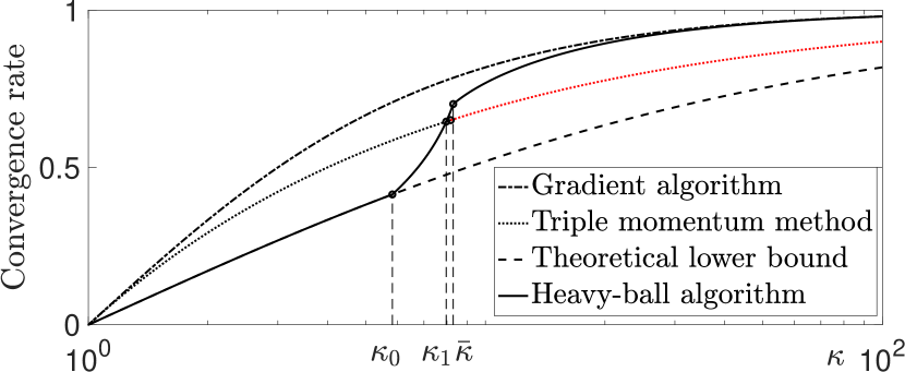
Figure 4: Graphs of $r^{*}$ (the solid line) and the optimal convergence rates of the gradient algorithm (the dash-dot line) and the triple momentum method (the dotted line, extension beyond $\kappa_{\mathrm{TM}}$ is shown in red). The theoretical lower bound $r_{\mathrm{P}}$ is also shown (the dash line).

V Conclusions and Future Work

We introduced the GHB parameters that lead to a globally convergent heavy ball method while simultaneously minimizing an upper bound on the $R$-convergence of the algorithm for solving a class of non-convex optimization problems. We showed that the triple momentum method is not guaranteed to be globally converging for all the functions in the same class and identified a family of functions in the class that the heavy ball method with GHB parameters enjoys a faster convergence property than the triple momentum method. Possible future directions include extending the result to constrained problems and the cases where a stochastic approximation of the gradient is available. It is also interesting to find constructive conditions on $f$ which imply (3). Another avenue of research is to use more sophisticated nonlinear stability analysis tools to obtain tighter upper bounds for the $R$-factor of the algorithm.

References

- [1] A. Ben-Israel and B. Mond. What is invexity? The ANZIAM Journal, 28:1–9, 1986.
- [2] F. F. Bonsall and M. Marden. Zeros of self-inversive polynomials. Proc. of the American Math. Society, 3(3):471–475, 1952.
- [3] E. Ghadimi, H. R. Feyzmahdavian and M. Johansson, Global convergence of the heavy ball method for convex optimization. In 2015 European control conference (ECC), pp. 310–315, July 2015.
- [4] W. M. Haddad and D. S. Bernstein. Explicit construction of quadratic Lyapunov functions for the small gain, positivity, circle, and Popov theorems and their application to robust stability. Part II: Discrete-time theory. Int. J. Robust Nonlin. Contr., 4:249–265, 1994.
- [5] W. M. Haddad and V. Chellaboina. Nonlinear dynamical systems and control: a Lyapunov-based approach. Princeton Univ. Press, 2008.
- [6] H. K. Khalil. Nonlinear systems. Prentice Hall, Upper Saddle River, third edition, 2002.
- [7] L. Lessard, B. Recht, and A. Packard. Analysis and design of optimization algorithms via integral quadratic constraints. SIAM Journal on Optimization, 26(1):57–95, 2016.
- [8] S. Michalowsky, C. Scherer, and C. Ebenbauer. Robust and structure exploiting optimization algorithms: an integral quadratic constraint approach. International Journal of Control, pages 1–24, 2020.
- [9] I. Necoara, Yu. Nesterov, and F. Glineur. Linear convergence of first order methods for non-strongly convex optimization. Mathematical Programming, 175(1):69–107, 2019.
- [10] Y. Nesterov. Lectures on convex optimization. Springer, 2018.
- [11] J. M. Ortega and W. C. Rheinboldt. Iterative solution of nonlinear equations in several variables. SIAM, 2000.
- [12] B. T. Polyak. Some methods of speeding up the convergence of iteration methods. USSR Comp. Math. and Math. Physics, 4(5):1–17, 1964.
- [13] B. T. Polyak. Introduction to optimization. Optimization Software, Inc., NY, 1987.
- [14] C. Scherer and C. Ebenbauer. Convex synthesis of accelerated gradient algorithms. 2021. arrXiv:2102.06520.
- [15] D. D. Šiljak. Algebraic criteria for positive realness relative to the unit circle. J. Franklin Inst., 295(6):469–476, 1973.
- [16] B. Van Scoy, R. A. Freeman, and K. M. Lynch. The fastest known globally convergent first-order method for minimizing strongly convex functions. IEEE Control Systems Letters, 2(1):49–54, 2018.