solidfmm: A highly optimised library of operations on the solid harmonics for use in fast multipole methods
Abstract.
We present solidfmm, a highly optimised C++ library for the solid harmonics as they are needed in fast multipole methods. The library provides efficient, vectorised implementations of the translation operations M2M, M2L, and L2L, and is available as free software. While asymptotically of complexity , for all practically relevant expansion orders , the translation operators display an empirical complexity of , outperforming the naïve implementation by orders of magnitude.
1. Introduction
1.1. Summary
solidfmm is a highly optimised C++ library for operations on the solid harmonics as they are needed in fast multipole methods.
-
•
Supports both single and double precision.
-
•
Fully vectorised on x86 CPUs with support for AVX or AVX-512.
-
•
Hand-written assembly implementations for maximal performance of critical parts.
-
•
Supports mixed order translations: you can do M2M, M2L, L2L with differing input and output orders. This is important for adaptive, variable order fast multipole codes.
-
•
Translations support arbitrary shift vectors.
-
•
No dependence on external libraries except for the C++ standard library.
-
•
Thread safe and exception safe.
-
•
Lean. The library interface is very small and easy to use. We used encapsulation using handles to avoid dependence of user code on implementation details.
-
•
Free software. Licenced under the GNU General Public License as published by the Free Software Foundation, either version 3, or, at your option, any later version.
solidfmm is available from the author’s institution at https://rwth-aachen.sciebo.de/s/YIJFvSERVBiOkbc, or from GitHub.
1.2. Motivation and Background
The fast multipole method (FMM) (Greengard and Rokhlin, 1987) has been called one of the top ten algorithms of the 20th century (Cipra, 2000). It allows for approximate solutions of -body problems, namely the evaluation of:
| (1) |
where is the so-called kernel function, is the number of bodies with locations and associated masses or charges , . It is straightforward to see that a direct evaluation of this sum at all particle locations requires arithmetic operations, making this approach infeasible for large numbers of bodies . In contrast, the FMM computes approximations of (1) in only operations, resulting in dramatic speedups, where the accuracy can be controlled by the user.
This is achieved through the use of series expansions of the underlying kernel function . These expansions are truncated at a user-defined order , where increasing results in more accurate, but also more expensive computations: the hidden constant in the -complexity depends on and the type of expansion used. One of the most important kernel functions is the fundamental solution of the Poisson equation, i. e., up to a factor of , the function , . It can be used for both gravitational as well as electrical potentials. The solid harmonics have been specifically derived with this particular kernel in mind and yield the most efficient expansions available. Expansions in their terms require only coefficients, compared to for Chebyshev or Cartesian Taylor expansions at the same level of accuracy. Depending on the application, common values for lie between for fast, low-fidelity computations and to satisfy the highest accuracy demands. Thus, by modern standards, an individual expansion is ‘small’, and millions of such expansions can be stored in the memory of even cheap hardware.
There are two different kinds of expansions in FMMs: mutipole and local expansions, also called M- and L-expansions, respectively. In the so-called M2L-translation,111Strictly speaking, the term ‘translation’ is a misnomer as it also involves a conversion. Yet, the name got stuck and is now commonly used in the context of FMMs. an M-expansion around one point is converted into an L-expansion around another point . This operation is without doubt the most crucial element of FMMs, for large it is required millions of times and most of the computational effort lies in this stage. The direct implementation of the M2L-translation has complexity . This number is not at all that small anymore when and millions of such operations are necessary. For this reason, several so-called ‘fast translation’ schemes have been devised reducing this complexity to or even .
On the one hand, many of the commonly available FMM software projects focus on the difficult task of creating an implementation that efficiently scales to highly parallel super-computers. Very elaborate techniques are used to minimise communication, handle load balancing, and to additionally make use of GPUs when available. On the other hand, the M2L-translation in these software packages is often implemented using simple, nested loops without further optimisation. ExaFMM (Yokota, 2013), for example, uses the straight implementation222See https://github.com/exafmm/exafmm/blob/master/kernels/laplace.h and additionally uses the trigonometric functions to evaluate the solid harmonics in spherical coordinates—even though they can more easily be computed in Cartesian coordinates using only square roots and elementary arithmetic (Wang and LeSar, 1996). Such implementations thus leave an opportunity for improvement at the local, CPU level. For this reason we believe that even sophisticated codes like ExaFMM could directly benefit from an optimised implementation of the M2L translation.
The main reason for this situation is probably that implementing fast, efficiently vectorised translation schemes for the solid harmonics is quite challenging. To our knowledge there simply is no implementation of fast translation schemes that is free (as both in beer and in liberty) and vectorised. solidfmm aims to change this situation. It provides a fully vectorised implementation of an algorithm sketched by Dehnen (Dehnen, 2014) with highly optimised routines for current x86 architectures. Inspired by the BLIS (van Zee and van de Geijn, 2015), the performance critical parts are reduced to a handful of isolated and small ‘microkernels’ written in assembly language and compiler intrinsics, while the main part of the library is written in platform-independent standard C++. This extensible design allows us to add support for further CPU architectures in the future. In addition to the M2L, the library also features accelerated implementations of the other translations in FMM: M2M and L2L. The library is intended to be used the context of the aforementioned highly-parallel FMM frameworks, such that they immedialetely benefit from its optimisations.
In this article we will first summarise the basics of the M2L translation. The M2M and L2L translations are very similar in nature, and while also implemented in solidfmm, omitted here for brevity. We then continue with a very brief review of various acceleration techniques, before describing Dehnen’s approach in greater detail. We then describe how solidfmm implements a slightly modified version of his algorithm and finish with benchmarks comparing solidfmm to the simple, naïve implementation.
2. The M2L Translation
In this section we give a review of the M2L translation. After describing its plain, canonical formulation we give a short survey of different acceleration techniques, before describing the ideas behind the current, rotation-based approach in greater detail.
2.1. Canonical Formulation
M- and L-expansions of order , developed around respectively are functions of the following shape:
| (2) |
Here, and are complex-valued functions, respectively called the regular and singular harmonics, as defined in the appendix. The coefficients are also called multipoles, whereas the are simply called local coefficients.
For one always has . This ensures that the sums in (2) always take real values; additionally one only needs to store the coefficients with . Further space could be saved by noting that for the imaginary parts are always vanishing. However, the memory savings from this are only marginal and come at the cost of more complicated memory layouts. For this reason, in this work, we will also store .
Thus, an M- or L-expansion of order can be stored using complex, or real numbers in a ‘triangular shape’ as illustrated in Figure 1. Lacking a better name, we will call such a triangular arrangement of coefficients a solid. We thus have defined solids and harmonics.333For the rest of this work, we slightly deviate from the standard mathematical nomenclature, where the functions and themselves are called solid harmonics. For us, the functions are called harmonics; a set of their values at a specific point or a set of coefficients is called solid.
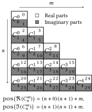 \Description
A triangular array that illustrates how coefficients of both M- and L-expansions are stored in memory.
Given a multipole expansion with coefficients and expansion centre , the corresponding local expansion at centre and with coefficients can be computed using the M2L-translation. It comes in two flavours:
| (3) |
respectively called the ‘single height’ and ‘double height’ kernels. These expressions only differ in the number of terms: for the double height kernel we need to compute up to order , while for the single height kernel order suffices. The single height kernel is cheaper, the double height kernel is more accurate. In its naïve implementation, the double height kernel is about six times more expensive to evaluate than the single height version (Coulaud et al., 2008, Footnote 5). This should be kept in mind when comparing implementations.
solidfmm implements the double height kernel, as it leads to more regular memory access patterns: every entry in linearly depends on every entry in . Thus, M2L can be interpreted as a linear mapping, i. e., a fully populated matrix, whose entries depend on the shift vector .
2.2. A Brief Survey of Fast M2L Schemes
Various approaches have been proposed to accelerate the M2L translation, a survey of the most common ones is given by Coulaud, Fortin, and Roman (Coulaud et al., 2008). Some of these approaches only work when there only is a finite set of shift vector directions , which is the case in certain implementations of the FMM. These approaches include:
-
•
BLAS-based approaches (Coulaud et al., 2008). These do not break the complexity. Instead, the finite set of translation matrices is stored explicitly, performance is achieved by using highly optimised BLAS routines to apply these matrices to many solids in parallel.
-
•
Plane-wave expansion methods (Greengard and Rokhlin, 1997). These only approximate the M2L translation and need careful tuning to match the accuracy of the original expansions for every given .
These schemes are unsuitable for use in solidfmm, which aims to be flexible and permit arbitrary shifts and orders .
Other, more general approaches include:
-
•
Diagonalising the translation matrix through the use of fast Fourier transforms (FFT) (Elliott and Board, 1996). These approaches achieve the aforementioned complexity of . However, practice has shown that they suffer from numerical instabilities for .
-
•
Rotation-based approaches (White and Head-Gordon, 1996). These perform a change of coordinates, after which the translation can be carried out in time. Finally, the result is changed back to the original coordinate system. Such changes of coordinates can also be done in time, resulting in the same overall complexity of .
There are approaches to repair the instabilities of the FFT method, but they all come at an extra cost. Additionally, we note that for , so for the stable choices of , whether the algorithmic complexity is favourable depends on the hidden constants and even more on the particular implementation. For these reasons solidfmm implements a rotation-based approach, which will be described in greater detail below.
2.3. Rotation-based Approaches
Rotation-based accelerations were introduced by White and Head-Gordon (White and Head-Gordon, 1996). The basic idea is as follows. Assume the shift-vector was aligned with the z-axis, i. e., assume we had . In this case, most of the entries in the M2L-kernels (3) vanish, because:
| (4) |
We now add a minor modification, by additionally assuming that . Then (3) reduces to:
| (5) |
In other words, for , M2L is an operation that acts column-wise on a solid, resulting in complexity. Thus, for the double height kernel, the general structure of the algorithm is as follows. Given solids of order and associated shift vectors , do the following:
-
(1)
Perform a change of coordinates on each , such that the shift is along .
-
(2)
For each column , perform the following matrix–matrix product:
(6) Note that real and imaginary parts do not couple! This matrix–matrix product can be carried out separately for real and imaginary parts. Also note that we apply the same matrix of faculties to all solids.
-
(3)
Apply the signs to the results.
-
(4)
Reverse the change of coordinates back to the original.
Here we see why we introduced the additional assumption : otherwise each solid would need to be multiplied with a different matrix. Now the the matrix is constant and identical for all solids . The matrix–matrix product (6) can be highly optimised using blocking techniques from the BLIS (van Zee and van de Geijn, 2015) and can be carried out separately for real and imaginary parts. However, to avoid wasting precious cache space, the matrix of faculties should not be stored explictly. It suffices to store the the values in a vector and write a specialised routine to carry out the product (6) using this vector.
Previous authors did not carry out the scaling to , and left the lengths of the shift vectors unchanged. In this case the necessary change of coordinates corresponds to a rotation, hence the name ‘rotation-based’. We will discuss different, but equivalent methods to achieve these rotations in the following subsection.
2.4. Rotating and Scaling Coordinate Systems
While M2L along the z-axis is an operation that acts column-wise on a solid, a change of coordinates acts row-wise. Scaling is trivial: when transforming a vector as for some , the M- und L-coefficients change as follows:
| (7) |
The cost of this operation is negligible. Letting the shift vector gets unit length, and it remains to perform rotations.
2.4.1. General Rotations
A general rotation takes the following form:
| (8) |
where the are the so-called Wigner matrices. These matrices depend on the Euler angles of the rotation in a highly non-trivial manner and its entries are very expensive to evaluate. For this, we refer to the original paper of White and Head-Gordon (White and Head-Gordon, 1996). If, however, only a finite set of shift directions is permitted, these matrices can be precomputed. Again, this makes this approach unsuitable for use in solidfmm, which aims to allow arbitrary shift vectors .
2.4.2. Factorisation of the Wigner Matrix
The idea of factorising the Wigner matrices into simpler matrices goes back to Wigner himself. It has long been known that rotations around the z-axis are trivial. For any angle , consider the transformation:
| (9) |
Under such rotations, the M- and L-coefficients transform as follows:
| (10) |
Wigner suggested precomputing the matrices for rotations by 90° around the -axis. This way, a general rotation can be carried out by combining three trivial rotations around the z-axis with two rotations by 90° around the -axis. In other words, we can make use of precomputed matrices for 90°, independent of the actual Euler angles of the rotation. Just like for the z-translation in (6), the same matrices are applied to all solids. The apparent drawback of this approach is that now two operations of the shape (8) are necessary instead of just one.
2.4.3. Dehnen’s Factorisation
Dehnen (Dehnen, 2014) picked up this idea in the context of M2L, and considered swapping the - and -axes instead. The corresponding matrices are denoted , resulting in the transformations
| (11) |
Swapping two axes turns a right-handed coordinate system into a left-handed one. However, because this operation is carried out twice, one obtains properly oriented results in the end. This approach has several benefits:
-
(1)
The matrices are involutory, i. e., they are their own inverses. Afterall, swapping x and z, and then swapping them again will get you back to where you started. There thus is no need to separately store the inverses.
-
(2)
All entries are real-valued. Thus, real and imaginary parts decouple in (11) and can be computed separately, cutting the operation count in half.
-
(3)
The matrices for the real and imaginary transformations are each only 50% populated. This reduces the cost of their application again by half and will be described in more detail later.
Thus Dehnen’s approach requires swapping the x- and z-axes twice, but each of these swaps only cost operations, making the approach competitive to precomputing the Wigner matrices for a set of fixed directions, but without the associated loss of generality.
2.4.4. Summary
In total, combining Dehnen’s approach with rescaling reduces the complexity of the M2L translation from to by factorising the operation into:
-
•
operations, namely the swapping of axes and translation along . These operations are ‘expensive’, but independent of the shift vectors. These operations can thus be vectorised and highly optimised by writing them as matrix–matrix products.
-
•
operations, namely scaling and rotations around the z-axis. These do depend on the shift vectors, but their cost is negligible. Additionally, vectorisation of these operations is even easier than vectorisation of the matrix–matrix products.
This approach is thus ideally suited for efficient implementations modern CPUs. Dehnen mentions that he implemented a vectorised version of this scheme, but to our knowledge his code is not freely available.
3. Implementation
3.1. Precomputation
The precomputation stage consists of computing the matrices required for swapping co-ordinate axes and storing them in a suitable memory layout. The computation of the faculties is trivial, and they can be stored in a simple vector. The matrices were introduced by Dehnen and we repeat his recurrence relations in the appendix. After these have been computed the corresponding matrices for the real and imaginary parts of solids can be computed. Using the facts that and , the mappings (11) become:
| (12) |
and analogous for . We thus define the swap matrices and , as follows:
| (13) |
With this, the mappings (11) turn into:
| (14) | ||||||
When storing the matrices and , as well as when implementing the mappings (14), it is important to notice that only 50% of their entries are non-zero. In particular the matrices exhibit a chequerboard pattern, as shown in Figure 2.
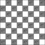
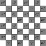
3.2. Blocking and Packing
The computationally most expensive parts of the M2L translation consist of dense matrix–matrix products. We can thus build on the experience of the BLIS (van Zee and van de Geijn, 2015) developers and apply blocking techniques. In particular, when forming a matrix–matrix product , the matrix is sub-divided into blocks of size , where the values of and are machine dependent. These blocks are then computed using the SIMD instructions of the processor, which are encapsulated in a so-called microkernel. A microkernel itself thus is machine specific, but it offers a generic, platform independent interface. The blocking scheme can thus be written using generic, platform independent code which then calls the machine specific microkernel to perform the actual computation. If necessary, and are padded by additional zero rows such that the total number of rows is a multiple of .
On many x86 systems supporting the AVX instruction set the optimal block size for double precision is and , where and are stored in row-major order. On a single core of such machines, we can thus process solids in double precision in parallel.444An AVX register can only hold four double precision values. However, most Intel microarchitectures since Haswell can simultaneously execute arithmetic instructions on two such registers in a single clock cycle, giving eight values in total. On systems supporting AVX-512 we choose and . Unlike the BLIS, we do not need to introduce an entire hierarchy of blocks that matches the cache hierarchy, as for realistic orders the swap matrices and are comparatively small and completely fit into the L2 and L3 caches of current CPUs.
While for the product (6) the matrix of the generic product can be compressed into a single vector of faculties, for the swap matrices and it is stored in the so-called packed format as illustrated in Figure 3.
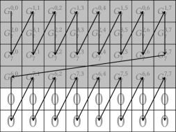
3.3. Buffers and Rearranging
Axis swap operations act row-wise on a solid and do not mingle real and imaginary parts. Thus, given solids and row , we need to compute the products:
| (15) |
In practice these matrices of real and imaginary parts will need to be stored in row-major order and padded with zero rows, such that the total number of rows is a multiple of . We thus need two buffers for holding these matrices, which are then filled with data from solids that may lie scattered in arbitrary positions in memory. We will call these the swap buffers.
On the other hand, the z-translation acts column-wise on a solid. In order to carry it out efficiently, we need to store the matrices:
| (16) |
for each ; padded and in row-major order. We will call these the translation buffers. In order to achieve maximum performance, it is thus necessary to copy data from the swap buffers into the translation buffers and vice versa. This is unfortunate, but there seems no way around this rearranging of data in memory.
Here the benefit of the row-major format becomes obvious. One row from a swap buffer corresponds to exactly one row in the corresponding translation buffer. We can increase performance by choosing such that one row corresponds to a fixed number of entire cache lines. For x86 systems with AVX support, this achieved by the choice for double precision: one row of these matrices then exactly corresponds to 64 bytes, the size of a cache line. We can thus always copy entire cache lines at once instead of proceeding element-wise in a scalar, non-vectorised fashion.
3.4. Summary: The Entire Algorithm
We now have gathered all the main ingredients of the algorithm implemented in solidfmm, and are in a position to summarise it here. Thus, let there be solids and shift vectors be given. We then proceed as follows, where for brevity we will omit the indices from now on:
-
(1)
For , and for each compute the following quantities: , , , . The exponential terms are powers of , , where:
(17) Thus, no trigonometric functions are necessary for this computation. Special care needs to be taken for when . In this case: and .
-
(2)
For each row :
-
(a)
Copy row from all of the solids into the swap buffers.
-
(b)
Scale and rotate around axis with angle :
-
(c)
Swap x- and z-axes:
(18) Only every other entry in the matrices , , is non-zero.
-
(d)
Rotate around axis by angle : (No scaling)
-
(e)
Swap - and -axes again, according to (18).
-
(f)
Copy the result into the translation buffers.
-
(a)
-
(3)
For each column : compute the matrix–matrix product (6), apply the signs .
-
(4)
For each row :
-
(a)
Gather row for each of the solids from the translation buffers and store them into the swap buffer.
-
(b)
Swap the - and -axes:
(19) Here the transposed matrices , are used.
-
(c)
Rotate around axis by the negative angle : (No scaling.)
-
(d)
Swap x- and z-axes again, according to equation (19).
-
(e)
Rotate around axis by and undo the scaling: Note that the denominator has power , not .
-
(f)
Store the result at the desired output location.
-
(a)
4. Performance Measurements
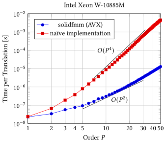
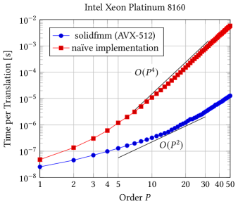
At the moment, solidfmm comes in version 1.2 with generic microkernels and optimised kernels for AVX and AVX-512. We consider the timings for the M2L kernel only, as it is the most crucial of the FMM’s translations. The benchmarks can be carried out using the executables benchmark_m2l and benchmark_m2l_naive for the accelerated and naïve implementations, respectively. These programmes carry out a large number of M2L translations for each order and measure the time needed to complete the task. Afterwards this amount of time is divided by the number of translations. The naïve implementation uses simple, four-fold nested loops to implement the double height kernel (3).
We carried out experiments on a single core of an Intel Xeon W-10885M, which supports AVX, and an Intel Xeon Platinum 8160, supporting AVX-512. The results are illustrated in Figure 4. The naïve implementation shows the expected complexity. solidfmm, on the other hand, performs faster than expected: we observe or better for all relevant orders, in contrast to the asymptotic complexity of . We believe that his is due to the following effects. The microkernels only achieve a fraction of their peak performance when applied to small problems. Thus, the growing complexity is compensated by higher computational efficiency. At the largest orders we then finally begin to see an increased slope. For the AVX-512 version one can clearly observe the effects of the blocking scheme with : at order the slope increases to about , another increase is visible at .
Already at we observe a 33-fold speed up for the Xeon Platinum 8160, while for the W-10885M it is 28. These numbers keep on increasing, at the respective speed ups are 124 and 94. We therefore believe that solidfmm is particularly interesting for high accuracy computations.
Acknowledgements.
This research was carried out under funding of the German Research Foundation (DFG), project ‘Vortex Methods for Incompressible Flows’, grant number 432219818. Without their support, this project would not have been possible. I also received funding from the German National High Performance Computing (NHR) organisation. I would also like to acknowledge the work of Simon Paepenmöller, one of my student workers. He helped in the development of preliminary software designs, and the tracking of many nasty sign bugs. This work is completely new, but draws from conclusions from these initial attempts and would not have been possible without them.Appendix
Here, for completeness, we repeat the recurrence relations as given by Dehnen (Dehnen, 2014).
Regular and Singular Harmonics
Let be given. Starting with and , one continues with the diagonal:
| (20) |
and then obtains the remaining entries via:
| (21) |
The Matrices
Starting with , one has:
| (22) |
where it is implicitly assumed that , whenever .
References
- (1)
- Cipra (2000) Barry A. Cipra. 2000. The Best of the 20th Century: Editors Name Top 10 Algorithms. SIAM News 33, 4 (May 2000).
- Coulaud et al. (2008) Olivier Coulaud, Pierre Fortin, and Jean Roman. 2008. High performance BLAS formulation of the multipole-to-local operator in the fast multipole method. J. Comput. Phys. 227, 3 (Jan. 2008), 1836–1862. https://doi.org/10.1016/j.jcp.2007.09.027
- Dehnen (2014) Walter Dehnen. 2014. A fast multipole method for stellar dynamics. Computational Astrophysics and Cosmology 1, 1 (2014), 1–23. https://doi.org/10.1186/s40668-014-0001-7
- Elliott and Board (1996) William D. Elliott and John A. Board, Jr. 1996. Fast Fourier Transform Accelerated Fast Multipole Algorithm. SIAM Journal on Scientific Computing 17, 2 (March 1996), 398–415. https://doi.org/10.1137/S1064827594264259
- Greengard and Rokhlin (1987) Leslie F. Greengard and Vladimir Rokhlin. 1987. A fast algorithm for particle simulations. J. Comput. Phys. 73, 2 (Dec. 1987), 325–348. https://doi.org/10.1016/0021-9991(87)90140-9
- Greengard and Rokhlin (1997) Leslie F. Greengard and Vladimir Rokhlin. 1997. A new version of the Fast Multipole Method for the Laplace equation in three dimensions. Acta Numerica 6 (Jan. 1997), 229–269. https://doi.org/10.1017/S0962492900002725
- van de Geijn et al. (2021) Robert A. van de Geijn, Margaret Myers, and Devangi Parikh. 2021. LAFF-On Programming for High Performance. ulaff.net. https://www.cs.utexas.edu/users/flame/laff/pfhp/
- van Zee and van de Geijn (2015) Field G. van Zee and Robert A. van de Geijn. 2015. BLIS: A Framework for Rapidly Instantiating BLAS Functionality. ACM Trans. Math. Software 41, 3 (June 2015), 1–33. https://doi.org/10.1145/2764454
- Wang and LeSar (1996) H. Y. Wang and R. LeSar. 1996. An efficient fast-multipole algorithm based on an expansion in the solid harmonics. The Journal of Chemical Physics 104, 11 (March 1996), 4173–4179.
- White and Head-Gordon (1996) Christopher A. White and Martin Head-Gordon. 1996. Rotating around the quartic angular momentum barrier in fast multipole method calculations. Journal of Chemical Physics 105, 12 (Sept. 1996), 5061–5067. https://doi.org/10.1063/1.472369
- Yokota (2013) Ryo Yokota. 2013. An FMM Based on Dual Tree Traversal for Many-Core Architectures. Journal of Algorithms & Computational Technology 7, 3 (Sept. 2013), 301–324. https://doi.org/10.1260/1748-3018.7.3.301