Evaluating natural language processing models with generalization metrics that do not need access to any training or testing data

Abstract

Selecting suitable architecture parameters and training hyperparameters is essential for enhancing machine learning (ML) model performance. Several recent empirical studies conduct large-scale correlational analysis on neural networks (NNs) to search for effective generalization metrics that can guide this type of model selection. Effective metrics are typically expected to correlate strongly with test performance. In this paper, we expand on prior analyses by examining generalization-metric-based model selection with the following objectives: (i) focusing on natural language processing (NLP) tasks, as prior work primarily concentrates on computer vision (CV) tasks; (ii) considering metrics that directly predict test error instead of the generalization gap; (iii) exploring metrics that do not need access to data to compute. From these objectives, we are able to provide the first model selection results on large pretrained Transformers from Huggingface using generalization metrics. Our analyses consider (I) hundreds of Transformers trained in different settings, in which we systematically vary the amount of data, the model size and the optimization hyperparameters, (II) a total of 51 pretrained Transformers from eight families of Huggingface NLP models, including GPT2, BERT, etc., and (III) a total of 28 existing and novel generalization metrics. Despite their niche status, we find that metrics derived from the heavy-tail (HT) perspective are particularly useful in NLP tasks, exhibiting stronger correlations than other, more popular metrics. To further examine these metrics, we extend prior formulations relying on power law (PL) spectral distributions to exponential (EXP) and exponentially-truncated power law (E-TPL) families.

1 Introduction

Selecting the optimal hyperparameters, such as those for training or model size, is a critical phase in the ML pipeline. Motivated by the importance of model selection, recent years have seen a wide array of large-scale empirical studies on the various metrics used to predict the test-time performance of ML models (Jiang et al., 2019; Dziugaite et al., 2020; Martin et al., 2021; Martin and Mahoney, 2021b). These generalization metrics have been applied in a wide variety of data science tasks, including predicting the quality of pretrained learning models (Martin et al., 2021; Martin and Mahoney, 2019), designing effective training procedures (Foret et al., 2020; Izmailov et al., 2018), improving network efficiency (Chen et al., 2020; Dong et al., 2019), quantifying model robustness (Yang et al., 2020; Tanay and Griffin, 2016), improving ensemble learning techniques (Garipov et al., 2018; Fort et al., 2019), analyzing and improving large-scale machine learning contests (Martin and Mahoney, 2021b), and so on. They are typically studied using correlational analysis, measuring how strongly each metric correlates with (and therefore, can predict) model performance. In this regard, several recent works point out the deficiencies of existing generalization metrics, including a lack of “robustness” to the changes of environmental hyperparameters (Jiang et al., 2019; Dziugaite et al., 2020) (such as data, neural network architecture and training schemes), or the Simpson’s paradox that generalization metrics perform differently (i.e., predict opposite trends) when applied to each sub-part of a collection of learning models or to the holistic study (Martin and Mahoney, 2021b). Another drawback is the over-reliance on CV models, which are relatively well-explored, and are not always representative of other types of tasks. With few exceptions (Nakkiran et al., 2019; Martin et al., 2021; Yang et al., 2021), systematic studies in other fields, such as NLP, are largely missing.

Generalization metrics for model selection in NLP. The objective of this work is to provide a systematic study of generalization metrics in NLP, addressing several deficiencies in prior studies (Jiang et al., 2019; Dziugaite et al., 2020; Martin et al., 2021). Compared to CV, model selection in NLP has several important differences that require careful consideration. For example, the training data from standard CV benchmarks can often be easily obtained, while large language model datasets are typically web-scale and are challenging to access. Therefore, generalization metrics that can assess the quality of learning models without access to data are ideal for NLP. In this paper, we focus on generalization metrics that do not need access to data, which is useful for evaluating pretrained NLP models (Wolf et al., 2020). Indeed, recent work has demonstrated that access to training or testing data should not be necessary for assessing the model quality of learning models (Martin et al., 2021), though these findings have yet to be evaluated at scale in the NLP domain. Furthermore, it is typically infeasible to train NLP models to interpolate the (frequently large) training set. Contrary to common practice for CV models, the training error on NLP datasets is often much larger than zero. This becomes an issue when applying most existing generalization metrics as they compare models through the generalization gap (i.e., the difference between training and test performance) rather than the test error itself. Metrics that focus on ranking the generalization gap include most of the well-known metrics in CV, such as those based on the PAC-Bayesian framework (Neyshabur et al., 2018; McAllester, 1999) and margins (Bartlett et al., 2017; Pitas et al., 2017; Jiang et al., 2018).

To illustrate the issue, consider selecting between two models with test errors $e_{1},e_{2}$, training errors $l_{1},l_{2}$, and generalization gaps $g_{1}=e_{1}-l_{1}$ and $g_{2}=e_{2}-l_{2}$. Assuming a generalization metric can rank the generalization gap perfectly (which is often the focus of prior studies on generalization metrics (Jiang et al., 2019, 2020; Dziugaite et al., 2020)) , we know only that one model has a larger training-test gap than another ($g_{1}>g_{2}$). For these two models, even if we have access to both models’ exact training errors $l_{1},l_{2}$, we still cannot determine which model exhibits smaller test error: if $l_{1}<l_{2}$, we cannot determine whether $l_{1}+g_{1}>l_{2}+g_{2}$ unless we know the training-test gaps $g_{1},g_{2}$ explicitly. Therefore, if our objective is to construct a metric that correctly predicts model performance, rank correlation with the generalization gap is insufficient. In this paper, we aim to study how generalization metrics rank correlate with model quality, for which we use test error as a close approximation. As we will demonstrate (in Figure 4), rank correlation with the generalization gap indeed does not imply rank correlation with model quality in practice, and in fact often orders models in the opposite order of their test errors. From a practical point of view, for NLP tasks, we prefer generalization metrics that can directly predict trends in test error (or similar evaluation metrics in NLP, such as the test BLEU score (Papineni et al., 2002)) rather than trends in the generalization gap.

Naturally, we cannot expect a metric to be universally correlated with test error if evaluating the metric does not need data. However, within certain classes of models (e.g., stages of training in one model or across pre-trained models), they may be effective at diagnosing model quality. With these objectives in mind, among the generalization metrics in the literature, we take particular interest in those derived from the heavy-tail self regularization (HT-SR) theory (Martin and Mahoney, 2019, 2021a) due to reasons summarized in the following:

In addition to these two advantages, actual data often follow heavy-tail distributions (Feldman, 2020; Martin and Mahoney, 2021a; Martin et al., 2021), which can be even more evident in NLP than the more well-behaved datasets in CV (Li, 2017) that are often used to study generalization.

HT-SR theory and shape metrics. The core principle of HT-SR theory is that HT structures arise naturally in the ESDs of the weight matrices as the result of extracting various correlations in data during optimization (Martin and Mahoney, 2021a, 2019, 2020; Martin et al., 2021; Martin and Mahoney, 2021b). Its primary practical consequence is that by estimating the PL coefficient from the ESDs (requiring only weights), one can predict model quality, as smaller coefficients are reported to correspond to higher test accuracy. However, these estimators can be unstable, and so one must be careful not to rely on them alone. The quality of the PL fit itself should also point to similar conclusions (Martin and Mahoney, 2021a), which can be a sanity check.

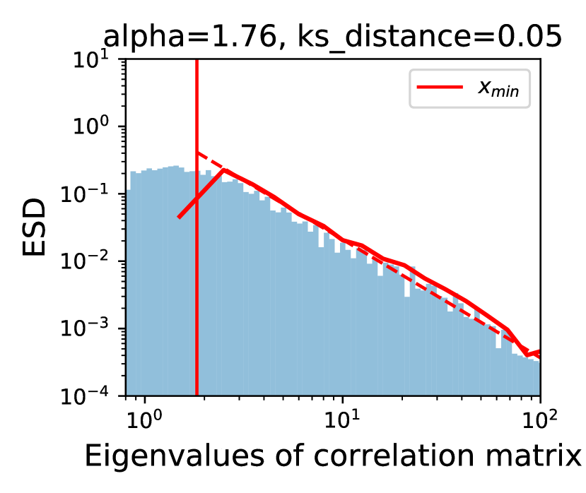
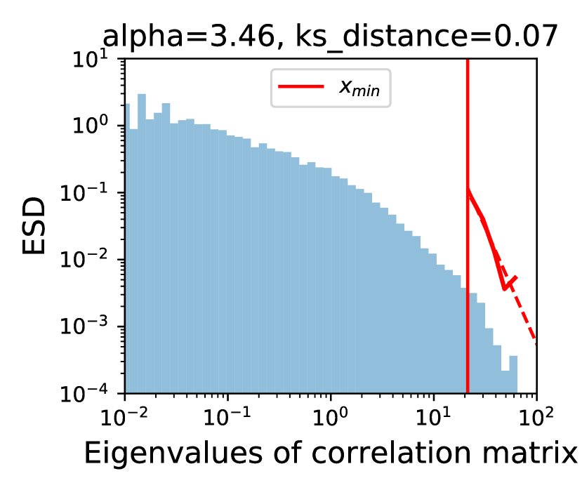
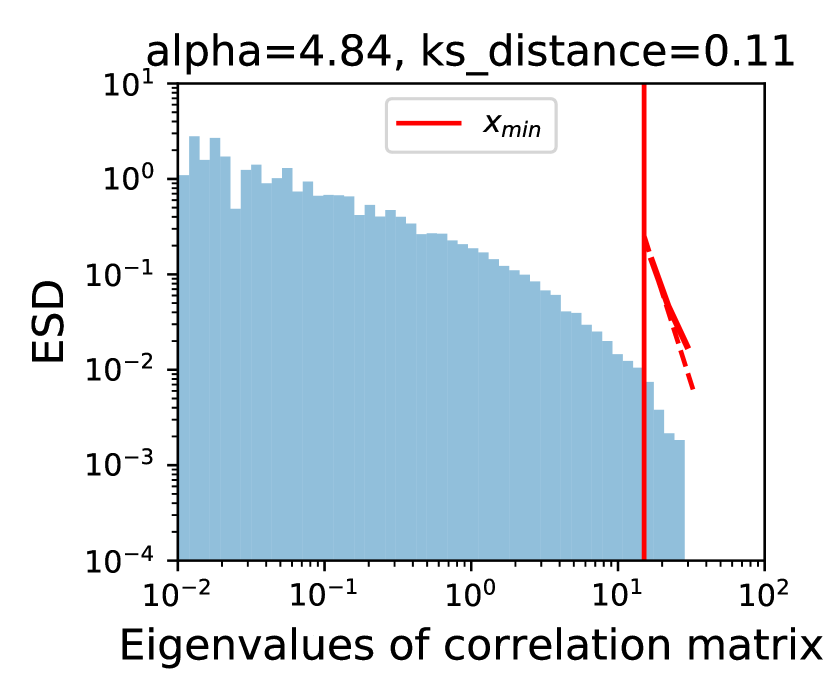
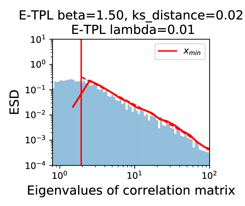
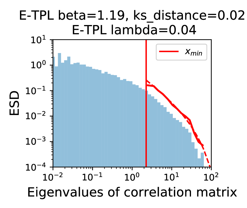
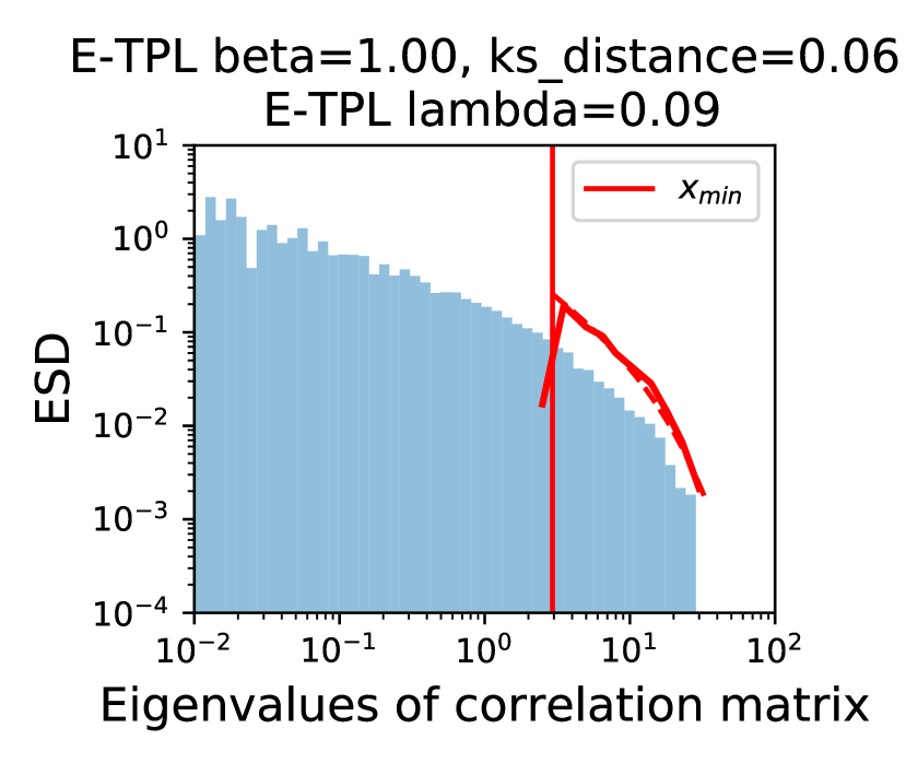
The principles of HT-SR theory extend beyond fitting the PL coefficient, however, as ESDs can take many forms. To this end, we study three different types of distributions to fit to the ESDs of weight matrices, including power laws (PL) in Eqn. (1), exponentially truncated power laws (E-TPL) in Eqn. (2), and exponential laws (EXP) in Eqn. (3). These are all commonly considered families of distributions in classical studies of PL (Clauset et al., 2009), and it is often hard in practice to predict which family fits data the best (as we show in this paper, this is true for deep NNs especially). Figure 1 shows examples of comparing different HT fittings on the same ESD. Following Martin and Mahoney (2021b), we refer to the various metrics derived from HT-SR as shape metrics.

(a) Small ks_distance.

(b) Mediocre ks_distance.

(c) Large ks_distance.

(d) E-TPL fitting of the ESD.

(e) E-TPL fitting of the ESD.

(f) E-TPL fitting of the ESD.

Figure 1: Comparing PL and E-TPL fitting. (First row). Good, mediocre, and bad PL fittings measured by the ks_distance. (Second row). E-TPL fitting of the ESD on the same column. Blue histograms represent the ESDs. Solid vertical lines represent the lower threshold $x_{\min}$ of the PL distribution found by the fitting procedure. Solid curves represent ESDs truncated using $x_{\min}$, and dashed curves represent the fitted HT distributions.

Contributions. The following summarizes our main contributions.

• Deviating from prior work examining generalization metrics in CV (Jiang et al., 2019; Dziugaite et al., 2020), we provide the first systematic correlational analysis on various generalization metrics in NLP. Our detailed studies include:

  • considering 360 transformers trained on WMT14 (Bojar et al., 2014) with varying hyperparameters, and eight families of pretrained SOTA transformers downloaded from Huggingface (Wolf et al., 2020), including BERT (Kenton and Toutanova, 2019), GPT2 (Radford et al., 2019), ALBERT (both v1 and v2) (Lan et al., 2019), etc;

  • providing the first systematic study of applying generalization metrics to the model selection of Transformers without any training/validation/testing data;

  • measuring the correlation between 28 generalization metrics and the model quality (measured by test-time performance) over three different model classes: (i) models trained with the optimal hyperparameters, (ii) a single model at different stages of training, and (iii) a model trained with different hyperparameters (similar to Jiang et al. (2019); Martin and Mahoney (2021b).)

  • corroborating results on multiple other datasets, including Wikitext-103, Reddit and MNLI; results using various ways of measuring rank correlations, including Spearman’s rank correlation and Kendall’s tau.

• We revisit prior findings on data-dependent metrics motivated by margins and PAC-Bayesian bounds (Jiang et al., 2019; Dziugaite et al., 2020), finding that while these metrics perform well in predicting the generalization gap, none of them satisfactorily predicts test error directly.

• When applied appropriately, we find that HT-based shape metrics consistently perform better than scale metrics (or norm-based metrics) for predicting model quality.

• We extend prior studies on HT-SR theory and investigate alternative models to fit heavy-tail/light-tail distributions. Our results show that E-TPL fits are comparatively robust alternatives to PL fits on suboptimally-trained models.

This technical report is an extended version of the conference paper (Yang et al., 2023). Compared to the conference version, this report provides full details of the correlational analysis when a single hyperparameter is changed (see Section 3.2.3). It also provides corroborating results on multiple other datasets and evaluation methods. In order that our results can be reproduced and extended, we have open-sourced our code.

Preliminary of ESDs of weight matrices.

Consider a NN with $d$ layers and corresponding weight matrices $\mathbf{W}_{1}$, $\mathbf{W}_{2}$,…, $\mathbf{W}_{d}$. For each weight matrix $\mathbf{W}_{i}$ with shape $N\times M$, assume without loss of generality that $N\geq M$ (otherwise, consider $\mathbf{W}_{i}^{\top}$). We define the correlation matrix as $\mathbf{X}_{i}=\mathbf{W}_{i}^{\top}\mathbf{W}_{i}$, and denote the eigenvalues of $\mathbf{X}_{i}$ as $\{\lambda_{j}\}_{j=1}^{M}$, so that $\lambda_{j}=\sigma_{j}^{2}$, where $\{\sigma_{j}\}_{j=1}^{M}$ are the singular values of $\mathbf{W}_{i}$. Furthermore, we use $\lambda_{i,\max}$ to denote the maximum eigenvalue of the correlation matrix $\mathbf{X}_{i}$. The ESD (empirical spectral density) of the weight matrix $\mathbf{W}_{i}$ refers to the empirical density of the eigenvalues of $\mathbf{X}_{i}$, typically represented through a histogram. We let $p(x)$ denote the density function to fit the ESD taking values in the interval $(x_{\min},x_{\max})$. For a power law, $p$ satisfies

$$p(x)\propto x^{-\alpha},\quad x_{\min}<x<x_{\max}.$$ (1)

From Martin and Mahoney (2021b), $x_{\max}$ is chosen to be the maximum eigenvalue of the empirical correlation matrix. However, $x_{\min}$ is a variable to be optimized to improve the quality of PL fitting, and it is not equal to the minimum eigenvalue in general.

2 Heavy-tail self-regularization

Here, we provide a brief overview of the HT-SR theory, and discuss several metrics that can be derived from it. According to HT-SR theory, the ESDs of the weight matrices become more heavy-tailed during training as they become increasingly correlated. One can quantify the extent of these correlations by fitting a PL to the ESD of a weight matrix, for example, by using the open-source WeightWatcher tool (Martin et al., 2021). After computing the ESD of a weight matrix, we use the maximum likelihood estimate from Alstott et al. (2014) to fit the PL distribution, the specific form of which has been defined in (1). Let PL_alpha denote the PL coefficient averaged over layers; effectively the slope of the tail of the ESD of the pooled weights, on a log-log scale.

Correctly identifying and fitting PL distributions is well-known to be a challenge in practice. For example, a density that appears as a straight line on a log-log scale plot need not follow a power law, as there are many other distributions that could show a similar behavior, including lognormal and exponential-type distributions (Clauset et al., 2009). Nested distributions such as E-TPL, which combine the pure PL and other distributional assumptions, can often improve the quality of fitting (Clauset et al., 2009; Alstott et al., 2014). Therefore, in addition to PL (defined in (1)), we consider several other distribution classes from the literature.

• (E_TPL_lambda and E_TPL_beta) The ESDs are assumed to take a “nested” form in the interval $(x_{\min},x_{\max})$.

  $$p(x)\propto x^{-\beta}\exp(-\lambda x),\,x_{\min}<x<x_{\max}.$$ (2)

  After fitting the E-TPL, we call the exponential truncation coefficient $\lambda$ the E_TPL_lambda metric, and we call the PL coefficient the E_TPL_beta metric.

• (EXP_lambda). The ESDs are assumed to take the following form, in the interval $(x_{\min},x_{\max})$.

  $$p(x)\propto\exp(-\lambda x),\,x_{\min}<x<x_{\max}.$$ (3)

  After fitting the EXP, we call the exponential coefficient $\lambda$ the EXP_lambda metric.

For more details of the various metrics considered in this paper, see Table 1. All of the metrics derived from HT-SR do not require access to data, nor do they require model training/retraining, and thus they are relatively cheap to compute. Our primary comparisons are between shape metrics (derived from HT-SR), and scale metrics (mostly norm-based). Scale metrics are mostly studied in prior work (Jiang et al., 2019; Dziugaite et al., 2020), while shape metrics have received less attention. For the precise definitions of these metrics, see Appendix A.

Name	Eqn	Ref	Need initial weights?	Scale or shape	Need data?	Need gpu?	Predicting model quality or generalization gap?
param_norm	(4)	Jiang et al. (2019)	No	Scale	No	No	Generalization gap
fro_dist	(5)	Jiang et al. (2019)	Yes	Scale	No	No	Generalization gap
log_norm	(6)	Martin and Mahoney (2021a)	No	Scale	No	No	Generalization gap
log_spectral_norm	(7)	Martin and Mahoney (2021b)	No	Scale	No	No	Generalization gap
dist_spec_int	(8)	Jiang et al. (2019)	Yes	Scale	No	No	Generalization gap
path_norm	(9)	Neyshabur et al. (2015)	No	Scale	No	No	Generalization gap
mp_softrank	(10)	Martin and Mahoney (2021a)	No	Scale/Shape	No	No	Model quality
stable_rank	(11)	Martin and Mahoney (2021a)	No	Scale/Shape	No	No	Model quality
PL_alpha	(1)	Martin and Mahoney (2021a)	No	Shape	No	No	Model quality
E_TPL_beta	(2)	This paper WeightWatcher	No	Shape	No	No	Model quality
E_TPL_lambda	(2)	This paper WeightWatcher	No	Shape	No	No	Model quality
EXP_lambda	(3)	This paper WeightWatcher	No	Shape	No	No	Model quality
PL_ks_distance	(12)	Martin and Mahoney (2021a)	No	Shape	No	No	Model quality
E_TPL_ks_distance	(12)	This paper Martin and Mahoney (2021a)	No	Shape	No	No	Model quality
alpha_weighted	(13)	Martin and Mahoney (2021a)	No	Hybrid	No	No	Model quality
log_alpha_norm	(14)	Martin and Mahoney (2021b)	No	Hybrid	No	No	Model quality
inverse_margin	(17)	Jiang et al. (2019)	No	Scale	Yes	Maybe	Generalization gap
log_prod_of_spec_over_margin	(18)	Bartlett et al. (2017) Pitas et al. (2017)	No	Scale	Yes	Maybe	Generalization gap
log_sum_of_spec_over_margin	(19)	Bartlett et al. (2017) Pitas et al. (2017)	No	Scale	Yes	Maybe	Generalization gap
log_prod_of_fro_over_margin	(20)	Bartlett et al. (2017) Pitas et al. (2017)	No	Scale	Yes	Maybe	Generalization gap
log_sum_of_fro_over_margin	(21)	Bartlett et al. (2017) Pitas et al. (2017)	No	Scale	Yes	Maybe	Generalization gap
path_norm_over_margin	(22)	Neyshabur et al. (2015)	No	Scale	Yes	Maybe	Generalization gap
pacbayes_init	(25)	Neyshabur et al. (2017)	Yes	Scale	Yes	Yes	Generalization gap
pacbayes_orig	(26)	Neyshabur et al. (2017)	No	Scale	Yes	Yes	Generalization gap
pacbayes_flatness	(27)	Neyshabur et al. (2017)	No	Scale	Yes	Yes	Generalization gap
pacbayes_mag_init	(28)	Jiang et al. (2019)	Yes	Scale	Yes	Yes	Generalization gap
pacbayes_mag_orig	(29)	Jiang et al. (2019)	No	Scale	Yes	Yes	Generalization gap
pacbayes_mag_flatness	(30)	Jiang et al. (2019)	No	Scale	Yes	Yes	Generalization gap

Table 1: Overview of the generalization metrics considered in this paper. We focus on the shape metrics derived from the ESDs of weight matrices. Due to the space constraint, definitions of some metrics are presented in Appendix A.

Issues of PL fitting. It is well-known that subtle issues can arise when fitting the ESDs (Clauset et al., 2009; Alstott et al., 2014; Martin and Mahoney, 2017, 2021b). To best mitigate these issues in PL fits, we adopt the fitting strategies used in WeightWatcher (Martin and Mahoney, 2017). For example, as in Clauset et al. (2009), it is common to choose the lower threshold $x_{\min}$ which coincides with the best quality fit under the Kolmogorov–Smirnoff statistic (referred to as PL_ks_distance for PL and E_TPL_ks_distance for E-TPL in the sequel; see Eqn. (12)). However, this method is time-consuming, especially for E-TPL as there are two parameters to fit. Instead, we adopt the fix-finger method (see WeightWatcher) which selects $x_{\min}$ as the peak of the ESD when fitting E-TPLs. More than a simple speed improvement, we find this method also yields more stable results.

Comparing PL and E-TPL fitting. Referring to Figure 1, we now discuss how E-TPL could partially address these fitting issues. On the first row of Figure 1, we show three typical cases of PL fitting. In Figure 1(a), the log-log scale reveals a “linear region” of the histogram, which the PL fitting correctly locates. The quality of fit, measured by the ks_distance, is within a typical range, as reported in Table 6 of Martin and Mahoney (2021a). In Figure 1(b) and Figure 1(c), the ESDs do not exhibit a clear linear region on the log-log scale. Following Martin and Mahoney (2021a), it is ill-advised to consider metrics derived from a PL fit in these scenarios. In practice, this typically occurs when PL_alpha $>4$ (e.g., see Figure 1(c)). On the other hand, in these two cases, the corresponding E-TPL fits (shown on the second row in Figure 1) still closely match the empirical density function (see Figure 1(e) and Figure 1(f)), and the ks_distance on the second row using a E-TPL fit is smaller than that for the PL fit on the first row, even when the fit on the second row clearly covers a larger part of the ESD. In these two cases, the E_TPL_lambda plays a similar role as the PL_alpha in PL fitting, and provides an effective alternative when the ESD does not exhibit a proper PL.

3 Empirical results

Figure 2: BLEU-score vs. six shape metrics for 200 Transformers trained on WMT14 with varying hyperparameters. HT-SR theory applies for optimally-tuned models (black stars), that is, for optimally-tuned models indicated by the black stars, models that have better BLEU scores exhibit heavier-tailed ESDs. HT-SR theory is a predictive theory designed to provide predictions for state-of-the-art-models (Martin and Mahoney, 2021a; Martin et al., 2021); thus, for suboptimal models, the HT-SR metrics can be anti-correlated with model quality, see e.g. the grey dotted line in the first subfigure.

In this section, we first give full details of the experimental setup, in Section 3.1. Then, we provide the analyses of the empirical results: in Section 3.2, we study Transformers trained from scratch with different hyperparameters; and in Section 3.3, we focus on pretrained Transformers from the Huggingface website.

3.1 Experimental setup

Dataset. In Section 3.2, we study models trained on the WMT14 German to English (DE-EN) dataset (Bojar et al., 2014), commonly used as a benchmark for neural machine translation (Ott et al., 2018; Vaswani et al., 2017; Shen et al., 2020; Edunov et al., 2018). WMT14 consists of 4.5 million sentence pairs for training.

Hyperparameters. To conduct correlational analysis, and to capture the relationship between the generalization metrics and model quality in different settings, we vary several hyperparameters: the number of samples (either 160K, 320K, 640K, 1.28M, 2.56M samples), the initial learning rate during training (across eight different rates), the model width (embedding dimension either 256, 384, 512, 768, or 1024), and the model depth ({4, 5, 6, 7, 8}-layer transformers). Similar to prior works on correlational analysis (Jiang et al., 2019) for model selection, we construct a high-dimensional grid of different hyperparameters $\mathbf{\Theta}=\{(\theta_{1},\ldots,\theta_{K}):\theta_{1}\in\mathbf{\Theta}_{1},\ldots,\theta_{K}\in\mathbf{\Theta}_{K}\}$, so that we can compare models when one of the hyperparameters is varied. Two separate high-dimensional grids with dimension $K=3$ are considered: (1) sample$\times$learning rate$\times$width; (2) sample$\times$learning rate$\times$depth. Each grid contains 5$\times$8$\times$5=200 of these training settings. In total, there are 360 trained models because the two high-dimensional grids overlap each other, and 40 models belong to both grids. We will conduct three correlational analyses in the following to evaluate model selection performance.

Task one, correlation evaluated on optimally trained models. In the first task (Section 3.2.1), we measure the (rank) correlation between model quality and generalization metrics on models trained with the optimal choice of training hyperparameters, that is, if we are allowed to grid-search the best training hyperparameters, can we predict the best data size or model size parameters?

Task two, correlation in time. In the second task (Section 3.2.2), we track BLEU score and generalization metrics during training, assessing time-wise correlation to model quality. This task has been considered in the literature (Bartlett et al., 2017), and from a practical point of view, capturing the time-wise dependence during training could potentially lead to better early stopping and regularization methods.

Task three, correlation when a single hyperparameter is varied. In the third task (Section 3.2.3), we study the relationship between the model quality and the generalization metrics when a single hyperparameter is varied. Metrics that achieve a high (rank) correlation for all the hyperparameters are good candidates for model selection.

Training and model setup. For the details of training Transformers on WMT14, see Appendix B.

3.2 Correlational analyses on Transformers trained in different settings

In this subsection, we study 28 generalization metrics (with details provided in Table 1) and examine their correlations with BLEU score (Papineni et al., 2002), the most commonly used metric to evaluate machine translation . Note that BLEU score here is used as a close approximation of model quality, mimicking the role of test accuracy in image classification. We also consider correlation between these metrics and the generalization gap, defined as the BLEU score for training data subtracted by the BLEU score for test data. We intend to find generalization metrics that strongly correlate with model quality instead of the generalization gap.

3.2.1 Task one: Evaluating correlations on optimally trained models only

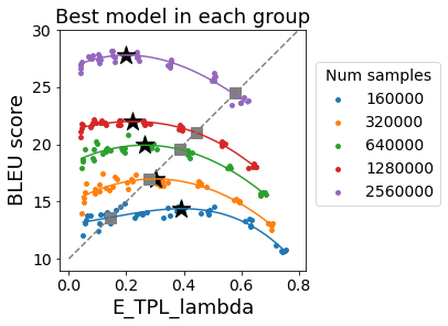
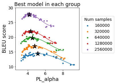
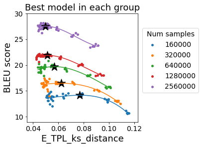
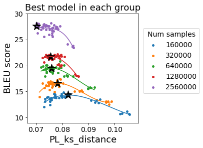
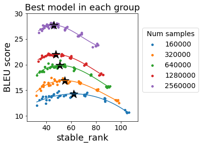
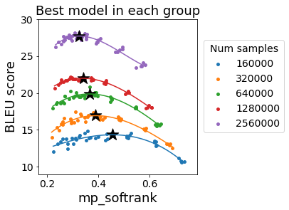
Here, we group models using the number of training samples, and select the best model from each group when the model depth and the learning rate are varied. In Figure 2, each curve represents a group of models trained with a certain number of training samples. The black star on each curve represents training with optimal hyperparameters (learning rate and depth in our setting), obtained by searching for the optimum on a third-order polynomial fit of each curve. From Figure 2, we see that the shape metrics correctly predict the model quality for models trained with the optimal training hyperparameters, i.e., the BLEU scores should be higher when the metric values are smaller on the optimal models represented using black stars. Since all six shape metrics show similar trends, a pairing of these metrics can be considered as a sanity check.

Comparison with scale metrics. We compare scale metrics and shape metrics in Section 3.2.3. We show that shape metrics predict the correct trends in test BLUE scores, while scale metrics predict wrongly because they are correlated with the generalization gap.

Remark 3.1.

Figure 2 points out an important but subtle issue in empirically evaluating the HT-SR theory. In Figure 2, one can make a model less well-trained—and artificially anti-correlate the generalization metric with the task accuracy. For example, see the gray dotted line in the first subfigure in Figure 2. In Section 3.3, we study models from the Huggingface website, and therefore, our results will strongly depend on how well-trained these models are.

3.2.2 Task two: Time-wise correlations and rank correlation results

Figure 3: E_TPL_lambda closely tracks the BLEU score, i.e., BLEU score increases when the E_TPL_lambda drops. Results are shown for Transformers trained on WMT14 with different number of samples. (First row). Training with dropout 0.1. (Second row). Training without dropout.

Correlations with model quality

(a) Correlations with model quality. Spearman’s rank correlation between various generalization metrics and BLEU.

Correlations with generalization gap

(b) Correlations with generalization gap. Spearman’s rank correlation between various generalization metrics and generalization gap.

Figure 4: Comparing multiple generalization metrics for predicting BLEU score (on the left) or the generalization gap (on the right). Lines on each box delineate the 25/50/75 percentiles of the rank correlations in 360 different settings (including different amount of data, different network depths, different network widths, and different initial learning rates).

In this subsection, we study time-wise correlation between our chosen metrics and the BLEU scores. In other words, we see if a generalization metric can track the test curve during training.

E_TPL_lambda tracks the BLEU score. As a warm-up, we consider how well the E_TPL_lambda metric defined in (2) tracks the BLEU score (recalling that E_TPL_lambda assumes the ESDs follow E-TPLs). We use training with and without dropout to study the effect of training schemes, and we consider different quantities of data to test robustness when the size of data changes. In Figure 3, the first row considers models trained with dropout, while the second row considers models trained without dropout. The multiple columns track E_TPL_lambda and the BLEU score throughout training for different amounts of data. We can see that E_TPL_lambda not only successfully tracks BLEU scores but also differentiates underfitting (first row, with dropout) from overfitting (second row, without dropout) in this experiment.

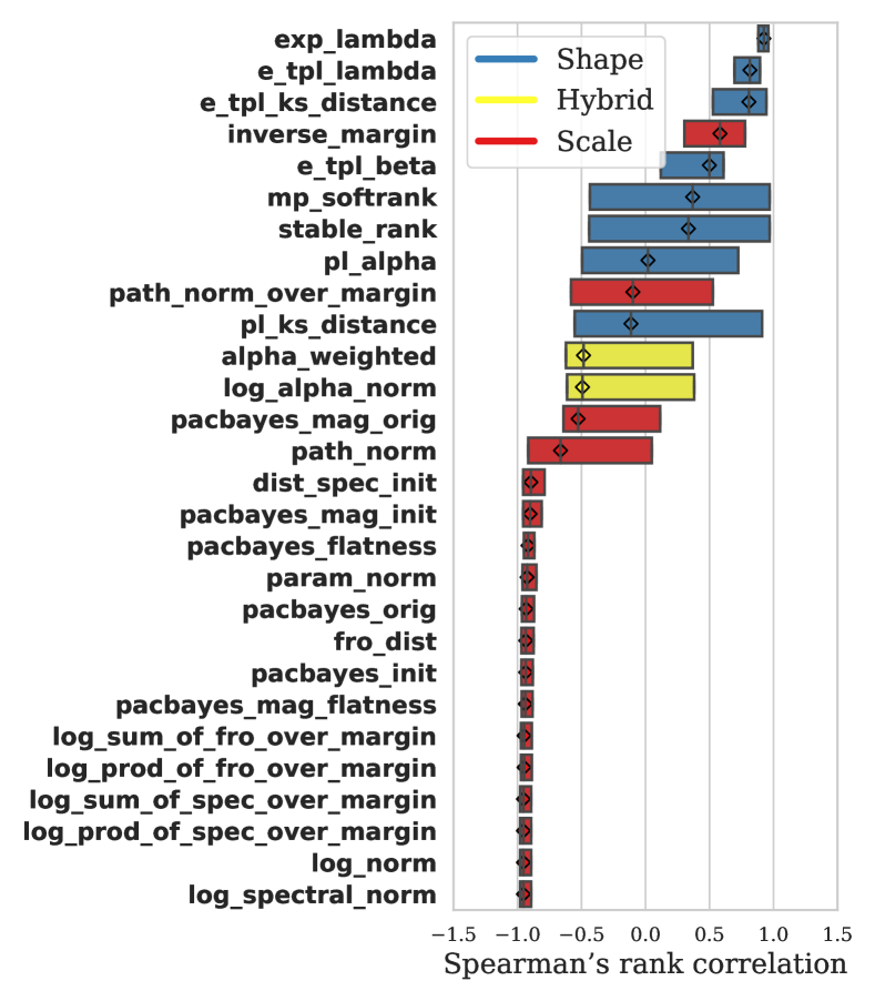
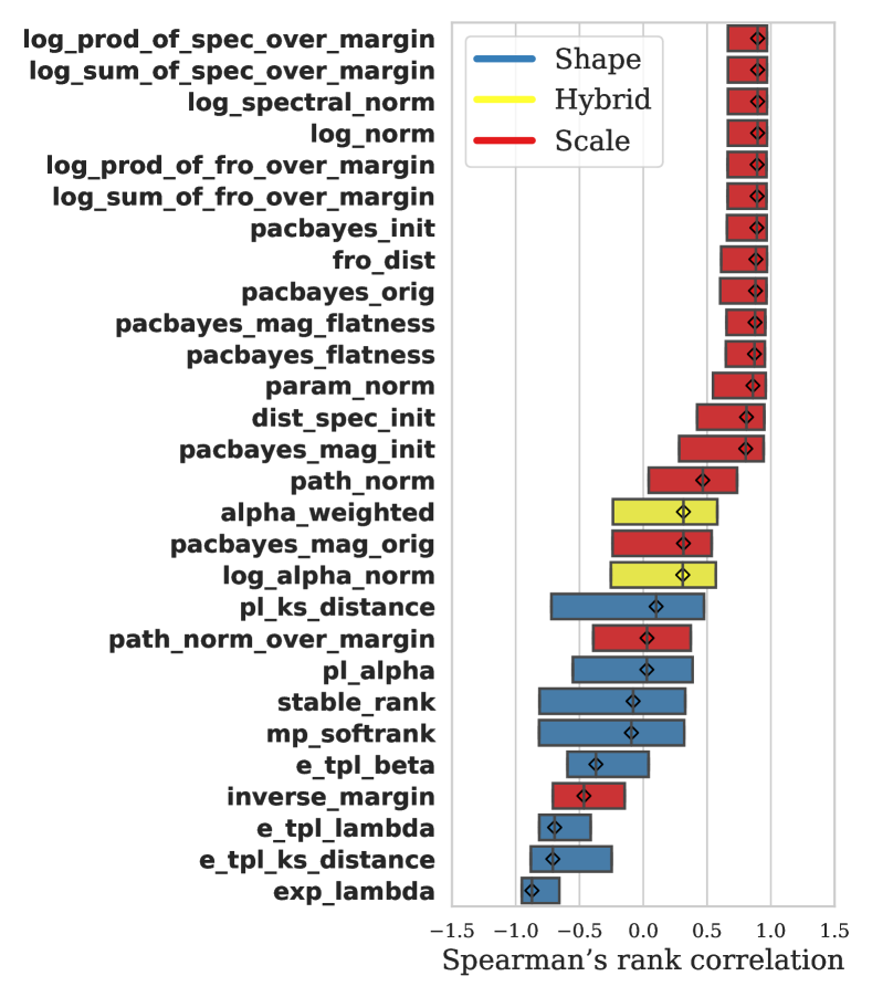
Shape metrics predict model quality, while scale metrics predict the generalization gap. Now we consider the rank correlations between our chosen metrics and the test BLEU score. The rank correlations are evaluated across training, i.e., for each of the 360 settings of the hyperparameters, we calculate the Spearman’s rank correlation between BLEU scores and the values of each generalization metric over all epochs. The summarized results are presented in Figure 4(a). A positive Spearman’s rank correlation (with BLEU) suggests that the generalization metric is useful in tracking BLEU during training. A negative Spearman’s rank correlation, on the other hand, implies that the metric often gives the incorrect prediction. In Figure 4(a), we use the average rank correlations for all settings to study the effectiveness of each metric, and present 25% quantile rank correlations to indicate robustness across runs.

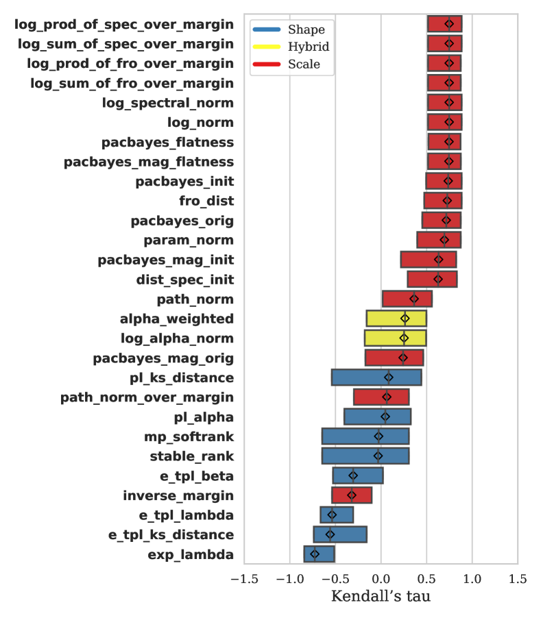
In Figure 4(a), we find shape metrics, such as E_TPL_ks_distance, EXP_lambda, E_TPL_lambda, and E_TPL_beta, exhibit some of the highest rank correlations with BLEU score. The EXP_lambda metric, which assumes a EXP distribution on the ESDs, achieves the highest median rank correlation, while the E_TPL_lambda metric, which assumes a E-TPL distribution on the ESDs, achieves the second highest. We discuss the inverse_margin metric in Appendix C.

In Figure 4(b), we plot the rank correlations to the generalization gap across our chosen metrics. While it is encouraging that most existing generalization metrics yield correct predictions, as previously discussed, correct predictions of the generalization gap do not imply accurate predictions on the best-performing models here.

Details of the rank correlation calculations. When calculating the rank correlation with the test accuracy, we associate a negative sign to all the generalization metrics, i.e., a positive rank correlation in Figure 4(a) means that a generalization metric is negatively correlated with the BLEU score. We use this procedure to follow the conventional wisdom that a smaller value of the complexity metric leads to better generalization (Jiang et al., 2019). On the other hand, for Figure 4(b), a positive rank correlation means that the metric is positively correlated with the generalization gap. Thus, for both Figure 4(a) and 4(b), a strong positive correlation corresponds to the expected trend.

Can we utilize anti-correlation for prediction? One may ask if the anti-correlation shown in Figure 4(b) implies that scale metrics can also predict model quality. Indeed, from Figure 4(b) alone, it seems that one can negate the predicted results of scale metrics to obtain an accurate prediction. However, note this strong negative correlation of scale metrics only holds in this one particular scenario. In other scenarios, such as in Jiang et al. (2019); Dziugaite et al. (2020), the correlation is strong in the other direction. Broadly speaking, if a particular theory says that a quantity should go up with model quality, and it goes down sometimes instead, then the theory is incomplete, regardless of how strong the correlation is. A prominent claim in our paper is that the correlation between test error and the generalization gap can sometimes be reversed. Therefore, it is insufficient to study metrics that have a large rank correlation with the generalization gap.

3.2.3 Task three: Rich correlational structures and the Simpson’s paradox when data size, model size and training hyperparameters are varied

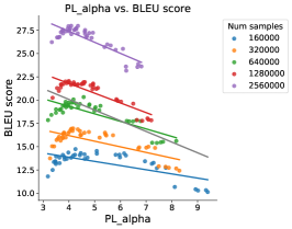
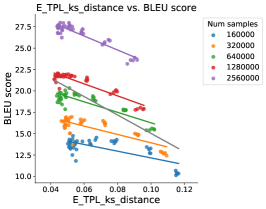
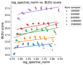
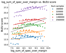
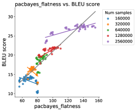
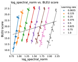
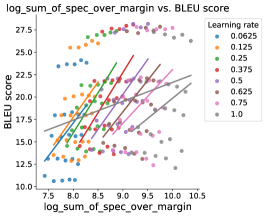
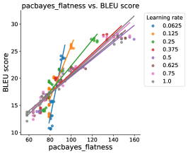
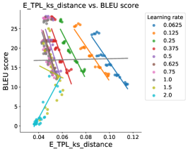
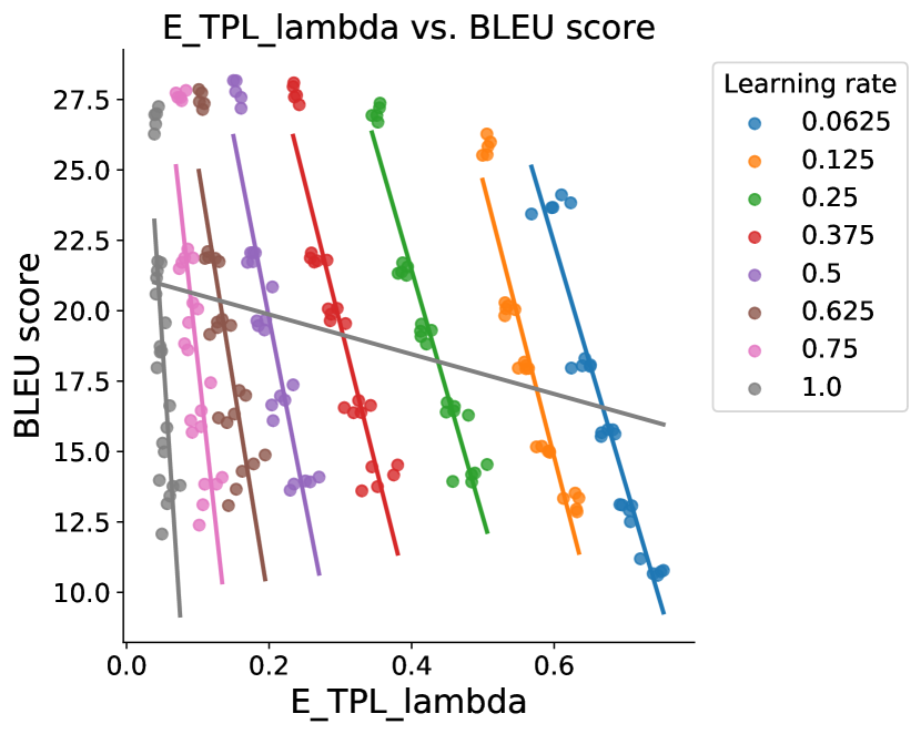
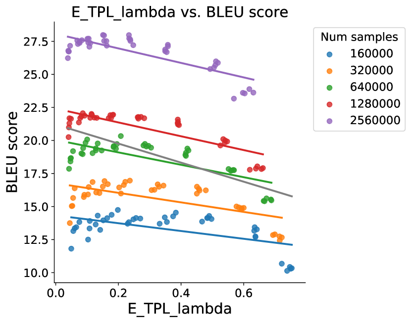
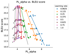
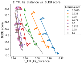
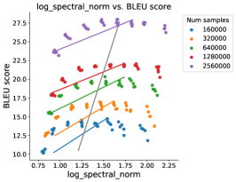
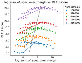
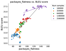
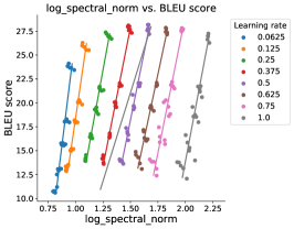
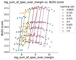
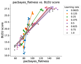
For our final task, we vary each of the hyperparameters and study the trends of the generalization metrics. We first focus on the sample$\times$learning rate$\times$depth hyperparameter grid— see Figures 5 and 6 for plots of BLEU score against shape and scale metrics, respectively. Since we vary the number of samples, the learning rate, and the model depth to obtain different models, we group these models to visualize trends over each hyperparameter. In each subfigure, we color-code the models by either learning rate or the number of samples. We discuss grouping models by depth later in Figure 8(c). Note that Figure 5 partially overlaps with Figure 2, except for different fitting methods.

For each curve, we expect the generalization metrics to be negatively correlated with the models’ quality measured using the BLEU score, i.e., the regression lines should have negative slopes. Comparing Figure 5 and 6, one can see that the shape metrics tend to show the correct trends (which are more negatively correlated) than the scale metrics.

Remark 3.2.

In Figure 5, constrained by the least-squares fitting, some regression lines are not aligned well with data, e.g., the second figure on the second row. In Appendix D, we fit the data using the orthogonal distance regression to mitigate this issue.

Abnormal hyperparameters lead to the “Simpson’s paradox”. From Figure 5, we can see that the prediction of trends degrades for relatively large learning rates. For a fixed number of samples, when the learning rate becomes larger, the trends deviate from a perfectly linear fit. Now, we include more models trained with particularly large learning rates, and we show the results in Figure 7. We see that the results potentially display a “Simpson’s paradox” (similar results for a different corpus of models have been reported previously by Martin and Mahoney (2021b)), i.e., the overall correlation trends are opposite to the trends in individual groups. In these figures, the regression lines are strongly influenced by the models trained with large learning rates and are biased towards the models with low BLEU scores. This phenomenon is known in the HT-SR literature (Martin and Mahoney, 2021b; Martin et al., 2021), and one often has to avoid biasing the results with these poorly trained models .

Figure 5: BLEU-score versus shape metrics for 200 Transformers trained on WMT14 with different hyperparameters. (First row) Trained models grouped by the number of samples. (Second row) Trained models grouped by the learning rate. The BLEU scores and the evaluated shape metrics display the correct (downward) trend.

Figure 6: BLEU-score versus scale metrics for 200 Transformers trained on WMT14 with different hyperparameters. (First row) Trained models grouped by the number of samples. (Second row) Trained models grouped by the learning rate. The BLEU scores and the evaluated shape metrics display the wrong (upward) trend.

Figure 7: BLEU-score versus shape metrics with particularly large learning rates. (First row). Trained models grouped by the learning rate. (Second row). Trained models grouped by the number of samples. The BLEU scores and the evaluated shape metrics display Simpson’s paradox when there are models trained with particularly large learning rates (1.5 and 2.0).

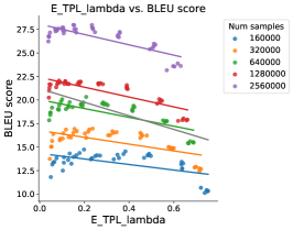
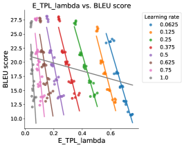
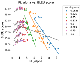
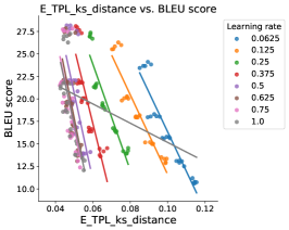
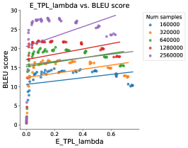
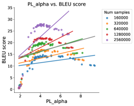
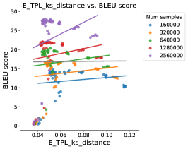
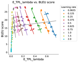
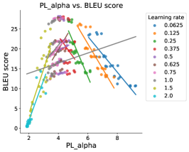
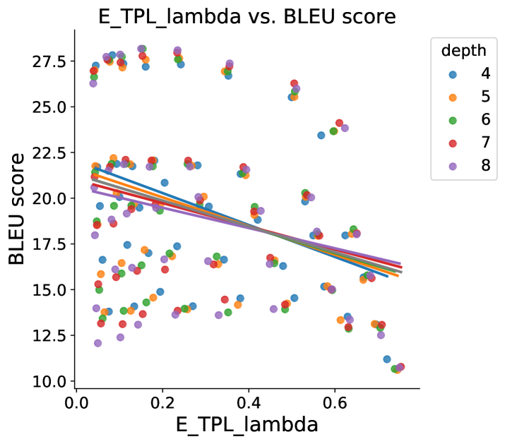
BLEU scores are not significantly influenced by network depth. Unlike learning rates and number of samples, we find that the BLEU scores are almost identical when we vary the number of layers from 4 to 8. In Figure 8(a) and 8(b), we show E_TPL_lambda vs BLEU for models grouped by different learning rates and number of samples. These two subfigures are repeated from the first column of Figure 7. From these two figures, we see that the BLEU scores vary significantly when these two hyperparameters are varied. In Figure 8(c), we show the same set of models color-coded by the network depth. We can see that the BLEU scores almost remain identical. This is because, from Figure 8(a) and 8(b), we see that these models are roughly divided into “vertical” groups when the learning rate is varied, and they are roughly divided into “horizontal” groups when the number of samples is varied. Therefore, each small “cluster” in Figure 8(c) corresponds to a group of models trained with the same learning rate and the number of samples but different depths, and these clusters show that the BLEU scores almost remain fixed when the depth is varied. This phenomenon suggests that the rank correlations calculated for varying depths may not be informative.

(a) Grouping by learning rates.

(b) Grouping by number of samples.

(c) Grouping by network depths.

Figure 8: E_TPL_lambda vs BLEU for the same set of trained models grouped by different hyperparameters. While BLEU scores change significantly when the initial learning rates and the number of samples are varied, they almost remain fixed for varying network depths.

Rank correlations. To systematically evaluate the various metrics considered in this paper, we study the rank correlation between these metrics and the BLEU score. For Task three, we consider each one-dimensional slice of the hyperparameter space $\mathbf{\Theta}=\{(\theta_{1},\ldots,\theta_{K}):\theta_{1}\in\mathbf{\Theta}_{1},\ldots,\theta_{K}\in\mathbf{\Theta}_{K}\}$, i.e., slices of the form

$$\{(\theta_{1},\ldots,\theta_{K}):\theta_{i}\in\Theta_{i}\text{ while other parameters $\theta_{j},j\neq i$ are fixed}\},$$

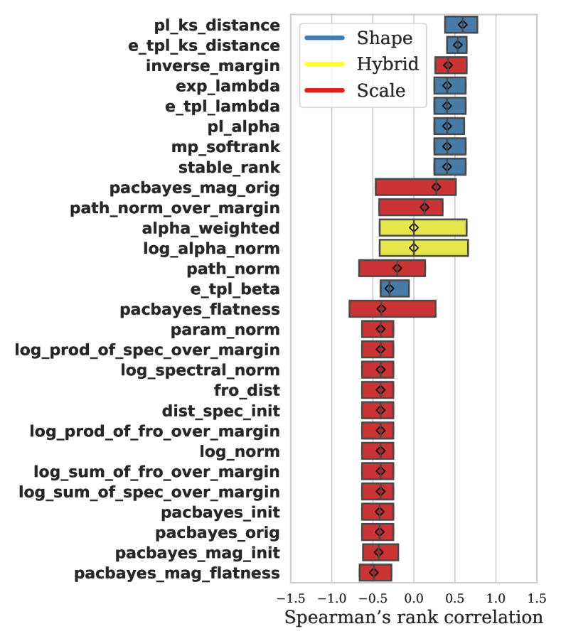
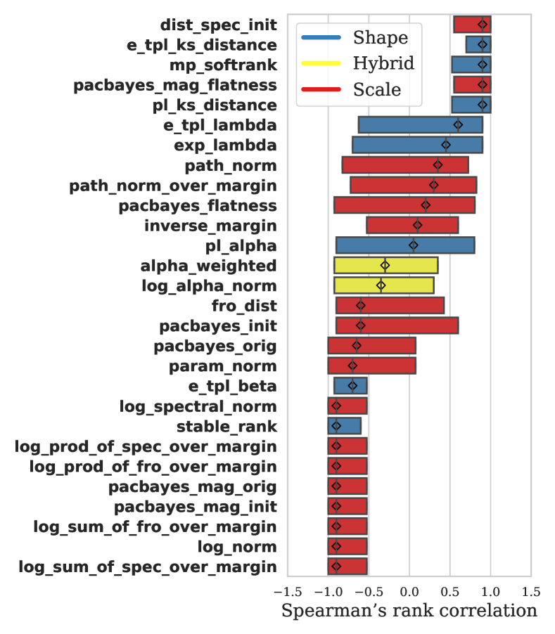
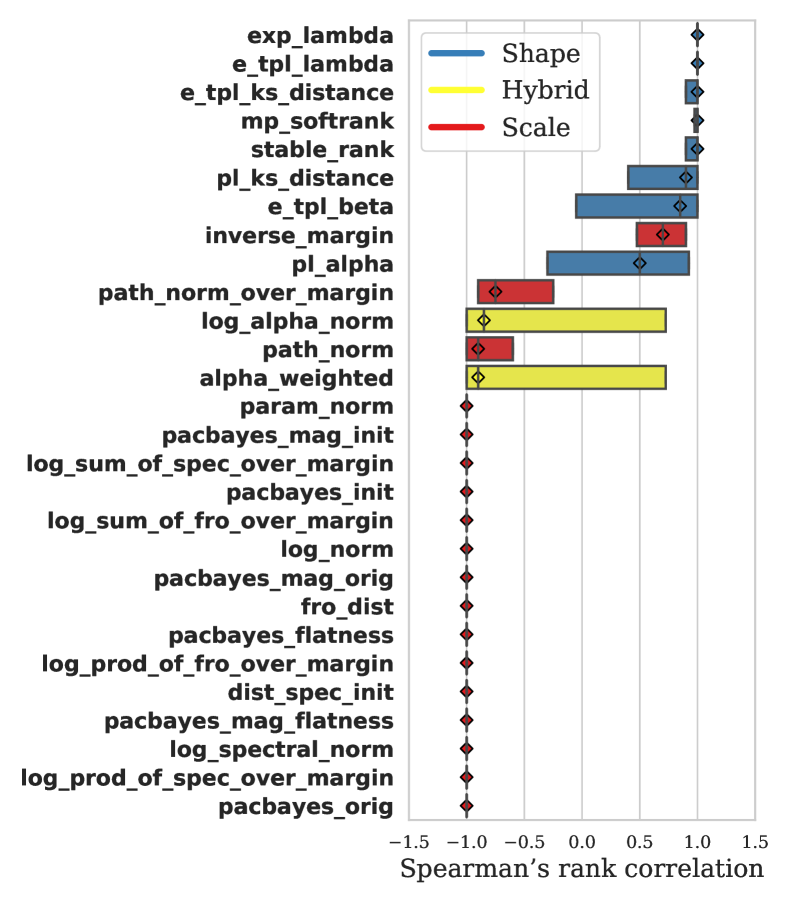
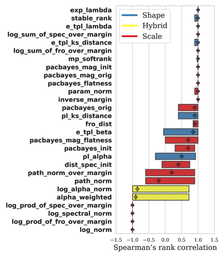
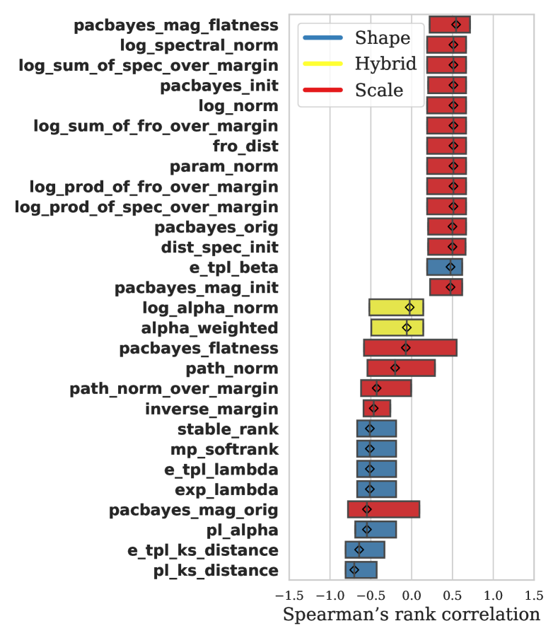
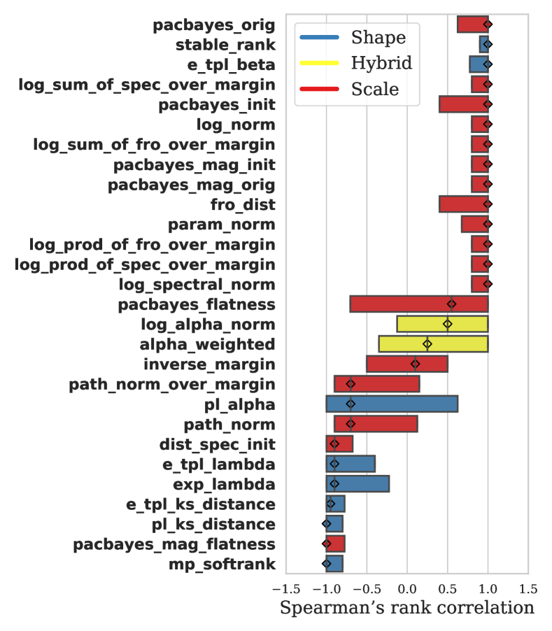
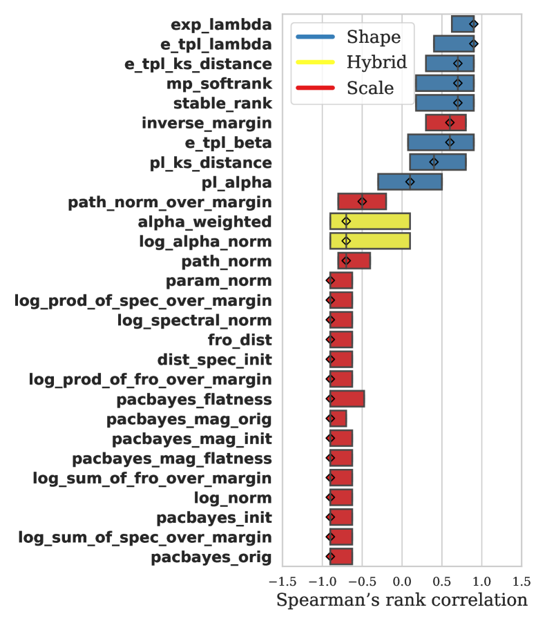
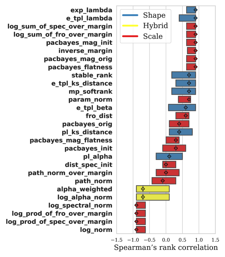
and we calculate the rank correlation using the models in each such slice. Then, we aggregate the rank correlations from all the one-dimensional slices and plot the distributions of the rank correlations. See Figure 9. As we have shown in Figure 8(c), the rank correlations calculated with varying network depths may not be informative due to the insignificant change in the BLEU score. Therefore, we focus on the other three hyperparameters, namely learning rate, network width and number of samples. Also, similar to Task two, we provide the rank correlation results on both the test BLEU scores and the generalization gap. Results on the generalization gap are shown in Figure 10.

Before we analyze the results of Figure  9 and 10, we discuss a subtle issue in calculating the generalization metrics. We note that, in Jiang et al. (2019), generalization metrics are “normalized” by dividing by the (square root of the) number of training samples, in correspondence with how they appear in uniform generalization bounds. However, normalizing the generalization metrics from Jiang et al. (2019) by the number of samples unavoidably complicates the correlation when varying the number of samples. This makes the comparison between scale metrics from Jiang et al. (2019) and the shape metrics challenging, as there is no natural way to normalize the shape metrics with respect to the number of training samples. Therefore, in Figure 9, we include the results for both with and without dividing the generalization metrics from Jiang et al. (2019) by the (square root of the) number of samples.

Here are our observations from Figure 9 and 10.

• From Figure 9(a) and 9(c), shape metrics perform particularly well when varying the learning rate and the number of samples. Specifically, in Figure 9(c), several shape metrics achieve perfect rank correlations, which are close to 1. From Figure 9(b), shape metrics also perform well for varying network widths except for stable_rank and E_TPL_beta .

• From Figure 9(d), normalizing the scale metrics from Jiang et al. (2019) by the number of samples significantly improves their correlational predictions. However, shape metrics can achieve a similar performance without the help of normalizing the number of samples.

• By comparing Figure 9 and 10, one can see that the scale metrics are much better correlated with the generalization gap than the test BLEU scores. For Figure 10(a) and 10(b), this conclusion is obvious from the plots. For Figure 10(c) and 10(d), the scale metrics need to be divided by (the square root of) the number of samples to achieve a good correlation when the number of samples is varied.

Correlations with model quality when different hyperparameters are varied.

(a) Varying learning rate.

(b) Varying network width.

(c) Varying number of training samples. In this subplot, metrics from Jiang et al. (2019) are not normalized by the number of training samples.

(d) Varying number of training samples. In this subplot, metrics from Jiang et al. (2019) are normalized by the number of training samples.

Figure 9: Comparing multiple generalization metrics in terms of the rank correlations with the test BLEU score when multiple hyperparameters are varied. Metrics are ranked by the median rank correlations.

Correlations with generalization gap when different hyperparameters are varied.

(a) Varying learning rate.

(b) Varying network width.

(c) Varying number of training samples. In this subplot, metrics from Jiang et al. (2019) are not normalized by the number of training samples.

(d) Varying number of training samples. In this subplot, metrics from Jiang et al. (2019) are normalized by the number of training samples.

Figure 10: Comparing multiple generalization metrics in terms of the rank correlations with the generalization gap when multiple hyperparameters are varied. Metrics are ranked by the median rank correlations.

Corroborating results. We extend our empirical evaluations to other datasets and evaluation methods. First, we consider pretrained Huggingface Transformers in Section 3.3, providing model selection results in a broad range of NLP tasks. Then, we consider three other language processing tasks trained with different Transformers, including

• Roberta (Liu et al., 2019) trained on the masked language modeling task using Wikitext-103 (Merity et al., 2016), and then finetuned on MNLI (Williams et al., 2018);

• Six-layer base Transformers trained on the language modeling task using the Wikitext-103 dataset (Merity et al., 2016);

• Six-layer base Transformers trained on the next-word prediction task using the Reddit dataset, following the implementation in Bagdasaryan et al. (2020).

All extended results can be found in Appendix E. Also, in Appendix E, we provide additional results on conducting correlational analysis using Kendall’s tau instead of Spearman’s rank correlation.

Computational cost and carbon emission. We believe it is extremely important that papers relying on large-scale empirical analysis accurately report the computational cost. The overall training cost is 7301.66 GPU hours. We use GPU nodes with TITAN RTX for our training. The overall carbon emission depends on carbon efficiency. Using the default values from the online Machine Learning Emissions Calculator, the total emissions are estimated to be 883.21 kg CO2 eq.

3.3 Selecting Huggingface Transformers

(a) Model selection on Huggingface Transformers. Metrics on the left and right are aligned.

(b) E_TPL_ks_distance evaluated on BERT models of different size.

(c) E_TPL_lambda evaluated on BERT models of different size.

Figure 11: Generalization metrics evaluated on pretrained Transformers. (a) Model selection results on eight Huggingface Transformer model series: BERT, GPT2, ALBERTv1, ALBERTv2, T5, DialoGPT, FlauBERT, Funnel Transformer. Left shows the rank correlation averaged over different Transformers. Right shows the proportion of the best Transformers correctly selected using different metrics. Shape metrics outperform scale metric only except stable_rank which is strongly influenced by the matrix size. (b and c) Evaluating two metrics on the “Smaller BERT” series. While E_TPL_ks_distance predicts the correct trends, E_TPL_lambda shows the reversed trends with depth.

Finally, we evaluate generalization metrics on the model selection task of pretrained Transformers. This section presents the first systematic study of applying generalization metrics to the model selection of Transformers without any training/validation/testing data. In our study, eight series of models downloaded from Huggingface (Wolf et al., 2020) are considered—see Table 2. We also include 24 BERT models from the “Smaller BERT” series (Turc et al., 2019) produced from a “pretrained distillation” pipeline that combines masked language modeling pretraining (Kenton and Toutanova, 2019) and knowledge distillation from a single BERT teacher model. In total, there are 51 pretrained Transformers.

Model series	Models
BERT (Kenton and Toutanova, 2019)	BERT {Tiny, Mini, Small, Base, Large}
Smaller BERT (Turc et al., 2019)	24 smaller BERT models (English, uncased,
	trained with WordPiece masking)
GPT2 (Radford et al., 2019)	GPT2 {Original, Medium, Large, XL}
ALBERTv1 (Lan et al., 2019)	ALBERT-v1 {base, large, xlarge, xxlarge}
ALBERTv2 (Lan et al., 2019)	ALBERT-v2 {base, large, xlarge, xxlarge}
T5 (Raffel et al., 2020)	T5 {small, base, large}
DialoGPT (Zhang et al., 2020)	DialoGPT {small, medium, large}
FlauBERT (Le et al., 2020)	FlauBERT {small, base, large}
Funnel Transformer (Dai et al., 2020)	FunnelModel {small, medium,
	intermediate, large, xlarge}

Table 2: Pretrained Transformers considered in this paper.

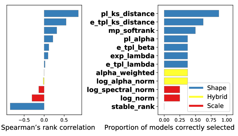
We report rank-correlations averaged over these 8 model series in Figure 11(a) (left subplot), i.e., larger/deeper models should have smaller generalization metric values. Again, we find that the shape metrics outperform scale metrics (except for stable_rank, which is strongly influenced by the size of the weight matrix). The hybrid models achieve performance in-between the shape and scale metrics. In Figure 11(a) (right subplot), we compare different metrics in their ability to select the best model. That is, we report for each metric the proportion that the best model is selected from one model series when this metric is used as the model selection criterion. Note that the rankings of metrics on the two subplots in Figure 11(a) are the same.

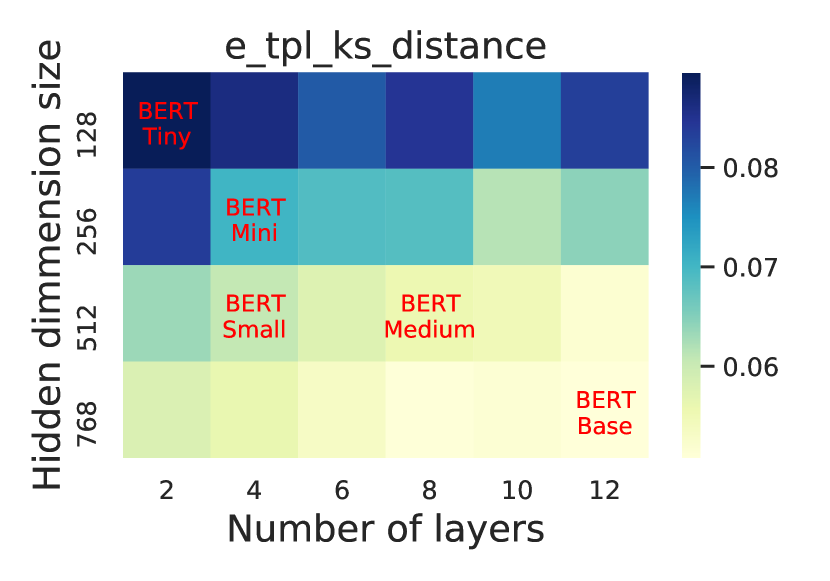
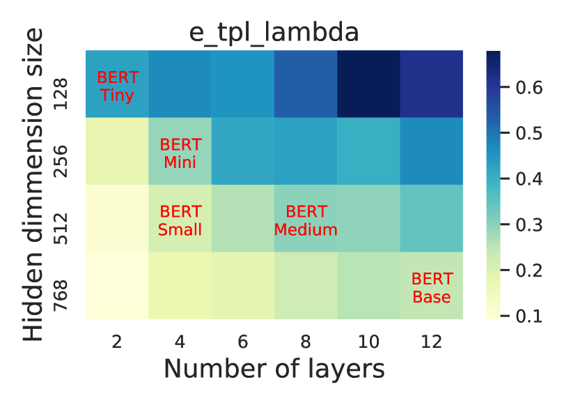
From Figure 11(a), we can see that, while the shape metrics perform better than scale metrics, none show a particularly strong rank correlation. To understand this, we examine the “Smaller BERT” series (Turc et al., 2019), which contains a more fine-grained structure of different model sizes. Specifically, these models are arranged in a 4-by-6 grid, where 6 represents {2,4,6,8,10,12} transformer layers and 4 means different hidden embedding sizes {128,256,512,768}. From Figure 11(b), we see that the E_TPL_ks_distance correctly predicts the trend that wider and deeper models perform better. On the other hand, from Figure 11(c), E_TPL_lambda correctly predicts that wider models are better, but incorrectly predicts that shallower models are better (yet another form of Simpson’s paradox in a data set of neural network model quality; see also Martin and Mahoney (2021b)). We note that the BERT series {BERT-Tiny, BERT-Mini, BERT-Small, BERT-Medium, BERT-Base, BERT-Large} overlaps with the 2D grid (as shown in Figure 11(b) and 11(c)). Consequently, the rank correlations for the BERT series (which we include as one of the eight series in making Figure 11(a), is a “noisy subsample” of the results in Figure 11(b) and 11(c).

Another curious observation from Figure 11(a) is that, for the pretrained transformers, PL metrics, such as PL_ks_distance and PL_alpha, outperform E-TPL metrics, such as E_TPL_ks_distance, E_TPL_lambda, and E_TPL_beta. This phenomenon may seem surprising as one may expect E-TPL fits to be more flexible than PL fits. These pretrained models are likely trained with much larger datasets and over many more epochs than the models we have otherwise considered. Here, PLs appear to provide a more natural fit. This is further evidence that HT-SR theory is particularly well-suited for evaluating the quality of relatively high-quality models.

4 Conclusion

Poor correlations between existing generalization metrics and test-time performance have been reported in prior work (Nagarajan and Kolter, 2019; Jiang et al., 2019; Dziugaite et al., 2020). Rather than providing a “lump sum” to rank existing and novel generalization metrics (Figure 4), we evaluated these metrics in several ways: quantifying correlations only on optimally-trained models (Figure 2); examining the time-wise correlation during training (Figure 3); differentiating between the correlation with test accuracy versus generalization gap (Figure 4); thoroughly investigating the rich correlational structures when different hyperparameters are varied (Figures 5 to 10); and evaluating these metrics on pretrained Transformer models where we do not have any control over the training process (Figure 11). Our large-scale empirical analyses suggest that popular generalization metrics still exhibit excellent correlations with generalization gap on NLP tasks. However, metrics derived from HT-SR theory appear to be most valuable to large language model practitioners, allowing one to assess pretrained NLP models without requiring training or testing data. Due to their apparent utility and current niche status, we recommend further investigations into these metrics, in particular, to address some of their remaining weaknesses (e.g. for suboptimally-trained models).

Acknowledgements. MM would like to acknowledge the IARPA (contract W911NF20C0035), NSF, and ONR for providing partial support of this work. KR would like to acknowledge support from NSF CIF-1937357, NSF CIF-2007669 and ARO fund 051242-002. JG would like to acknowledge supports from NSF CISE Expeditions Award CCF-1730628, NSF CAREER Award and gifts from Alibaba Group, Amazon Web Services, Ant Group, Ericsson, Facebook, Futurewei, Google, Intel, Microsoft, Nvidia, Scotiabank, Splunk and VMware. WeightWatcher is a publicly-available tool distributed under Apache License 2.0 with copyright held by Calculation Consulting. Our conclusions do not necessarily reflect the position or the policy of our sponsors, and no official endorsement should be inferred.

Appendix A Generalization metrics

In this section, we provide definitions and details on the various metrics considered in our analysis. We begin with scale metrics, and then consider shape metrics obtained from the ESDs of the weight matrices. Although our focus is on generalization metrics that do not need data to evaluate, we also define generalization metrics based on margin (Bartlett et al., 2017; Pitas et al., 2017) and PAC-Bayesian bounds (McAllester, 1999; Neyshabur et al., 2018).

A.1 Notation and preliminaries

General notation. As before, we consider a NN with $d$ layers and corresponding weight matrices $\mathbf{W}_{1}$, $\mathbf{W}_{2}$,…, $\mathbf{W}_{d}$. We use $\mathbf{W}$ to denote the collection of all the weights and denote the vector that consists of all the model weights as $\text{vect}(\mathbf{W})$. The neural network (as a function) is denoted by $f_{\mathbf{W}}$, taking a single input sample $\mathbf{x}$ and outputs a vector $f_{\mathbf{W}}(\mathbf{x})$. The superscript ${}^{\text{init}}$ on a weight matrix, e.g. $\mathbf{W}_{1}^{\text{init}}$, denotes the initial weights from which the model is trained. The notation $\mathbf{1}$ means an all-one vector, and $\mathbf{I}$ means the identity matrix.

Norms and distances. We use different types of norms defined on vectors and matrices. $\|\cdot\|_{2}$ and $\|\cdot\|_{1}$ used on vectors respectively means the $\ell_{2}$ norm and the $\ell_{1}$ norm. $\|\cdot\|_{F}$ and $\|\cdot\|_{2}$ used on matrices respectively denotes the Frobenius norm and the spectral norm (which is the induced $\ell_{2}$ norm).

A.2 Scale metrics

Norm-based and distance-based metrics. In the following, we discuss multiple metrics obtained from the norms of the weights or the distance between the final weights and those at initialization. While some metrics are averaged over layers, and others are not, this inconsistency is not in error. We follow definitions of metrics from several prior papers verbatim. Results in the second task (comparing model performance across a single training run) are independent of these factors. However, to compare networks with different sizes, proper normalization is necessary. Some metrics across the literature are also linearly dependent on others, and are therefore redundant for comparison. For example, log_prod_of_spec and log_sum_of_spec from Jiang et al. (2019) overlap with log_spectral_norm from Martin and Mahoney (2021b), and log_sum_of_fro and log_prod_of_fro from Jiang et al. (2019) overlap with log_norm from Martin and Mahoney (2021a). These metrics are not considered.

• (param_norm). The squared Frobenius norm summed over all weight matrices.

  $$\mu_{\text{{param\_norm}}}=\sum_{i=1}^{d}\|\mathbf{W}_{i}\|_{F}^{2}.$$ (4)

• (fro_dist). The distance between a weight matrix and its initilized value, calculated using the Frobenius norm and summed over all layers.

  $$\mu_{\text{{fro\_dist}}}=\sum_{i=1}^{d}\|\mathbf{W}_{i}-\mathbf{W}_{i}^{\text{init}}\|_{F}^{2}.$$ (5)

• (log_norm).

  $$\mu_{\text{{log\_norm}}}=\frac{1}{d}\sum_{i=1}^{d}\log\|\mathbf{W}_{i}\|_{F}^{2}.$$ (6)

• (log_spectral_norm).

  $$\mu_{\text{{log\_spectral\_norm}}}=\frac{1}{d}\sum_{i=1}^{d}\log\|\mathbf{W}_{i}\|_{2}^{2}.$$ (7)

• (dist_spec_int).

  $$\mu_{\text{{dist\_spec\_int}}}=\sum_{i=1}^{d}\|\mathbf{W}_{i}-\mathbf{W}_{i}^{\text{init}}\|_{2}^{2}.$$ (8)

• (path_norm). The metric is introduced in Neyshabur et al. (2015). To calculate the metric, we square the parameters of the network, perform a forward pass on an all-ones input and then compute the sum of the network outputs.

  $$\mu_{\text{{path\_norm}}}=\left\|f_{\mathbf{W}^{2}}(\mathbf{1})\right\|_{1}.$$ (9)

Scale metrics that require more shape information from the ESDs. The following metrics require more than just a single type of norm, instead involving a combination of a norm with other factors.

• (mp_softrank). This metric is introduced in Martin and Mahoney (2021a). To calculate this metric, we fit the MP distribution on the ESD, obtain the bulk max of the MP distribution and then divide by the maximum eigenvalue.

  $$\mu_{\text{{mp\_softrank}}}=\frac{1}{d}\sum_{i=1}^{d}\lambda_{i,\text{MP}}/\lambda_{i,\max}.$$ (10)

• (stable_rank). The metric is a norm-adjusted measure of the scale of the ESD.

  $$\mu_{\text{{stable\_rank}}}=\frac{1}{d}\sum_{i=1}^{d}\|\mathbf{W}_{i}\|_{F}^{2}/\|\mathbf{W}_{i}\|_{2}^{2}$$ (11)

A.3 Shape metrics

Tail-exponent fitting. The following metrics are derived from heavy or light-tailed fits to the ESD.

• (PL_alpha). The slope of the tail of the ESD, on a log-log scale. We use MLE from Alstott et al. (2014) to estimate PL_alpha. The distribution of eigenvalues is assumed to have the form of (1).

• (E_TPL_lambda). The tail exponent of the E-TPL fit to the ESD. This is a novel generalization metric introduced in this work.

• (EXP_lambda). The tail exponent of the EXP fit to the ESD, under the assumption that the ESD follows an exponential distribution (3). This is also a novel generalization metric introduced in this work.

• (PL_ks_distance). The Kolmogorov-Smirnoff (KS) goodness-of-fit test statistic for the PL fit:

  $$\mu_{\text{{ks\_distance}}}=\frac{1}{d}\sum_{i=1}^{d}\sup_{x}|F_{i}^{*}(x)-S_{i}(x)|,$$ (12)

  where $F_{i}^{*}(x)$ is the distribution of the estimated PL fit to the ESD, and $S_{i}(x)$ is the ESD itself.

• (E_TPL_ks_distance). The KS test statistic for the E-TPL fit, defined in the same way as (12), except that $F_{i}^{*}(x)$ is the distribution of the estimated E-TPL fit to the ESD.

A.4 Hybrid metrics

The following metrics are scaled versions of PL_alpha, involving both shape information from PL_alpha and scale information from other weighted norms. Let $\alpha_{i}$ denote the estimated PL coefficient of the ESD of the $i$-th weight matrix $\mathbf{W}_{i}$. Recall that $\lambda_{i,\max}$ is the largest eigenvalue of $\mathbf{W}_{i}$.

• (alpha_weighted). A scale-adjusted form of PL_alpha. This metric is denoted as $\hat{\alpha}$ in Martin and Mahoney (2021a); Martin et al. (2021); Martin and Mahoney (2021b).

  $$\mu_{\text{{alpha\_weighted}}}=\frac{1}{d}\sum_{i=1}^{d}\alpha_{i}\log\lambda_{i,\max}.$$ (13)

• (log_alpha_norm). This metric is another scale-adjusted PL_alpha metric in the form of a Schatten norm. Recall that we let $\{\lambda_{j}\}_{j=1}^{M}$ denote the set of eigenvalues of the correlation matrix $\mathbf{X}_{i}=\mathbf{W}_{i}^{\top}\mathbf{W}_{i}$, where $\mathbf{W}_{i}$ is the $N$-by-$M$ weight matrix that satisfies $N\geq M$. Then, we can define the Schatten $p$-norm as

  $$\|\mathbf{X}_{i}\|_{p}=\left(\sum_{j=1}^{M}\lambda_{j}^{p}\right)^{\frac{1}{p}}.$$ (14)

  The metric log_alpha_norm is given by

  $$\mu_{\text{{log\_alpha\_norm}}}=\frac{1}{d}\sum_{i=1}^{d}\log\|\mathbf{X}_{i}\|_{\alpha_{i}}^{\alpha_{i}}.$$ (15)

A.5 Margin-based metrics

Finally, we discuss generalization metrics derived from margins. Recalling that $f_{\mathbf{W}}$ denotes a neural network with weights $\mathbf{W}$, for a multi-class classification problem with sample-label pair $(\mathbf{x},y)$, we define the margin as

$$\gamma(\mathbf{x},y,f_{\mathbf{W}})=(f_{\mathbf{W}}(\mathbf{x}))[y]-\max_{i\neq y}f_{\mathbf{W}}(\mathbf{x})_{i}.$$ (16)

For machine translation, we consider the margin of each output token. We note that the number of classes, or the number of possible tokens, is often particularly large (in the order of thousands) for machine translation. Note that margins can be defined in any layer (Elsayed et al., 2018; Yang et al., 2020; Wei and Ma, 2019). Following Jiang et al. (2019), we consider output margins only, and use the 10${}^{\text{th}}$ percentile of the margin distribution calculated from the entire training set as a robust surrogate for the minimum margin. Using the margin $\gamma$ defined as the 10${}^{\text{th}}$ percentile, we define several generalization metrics.

• (inverse_margin).

  $$\mu_{\text{{inverse\_margin}}}=\frac{1}{\gamma^{2}}.$$ (17)

• (log_prod_of_spec_over_margin).

  $$\begin{split}\mu_{\text{{log\_prod\_of\_spec\_over\_margin}}}=\log\frac{\prod_{i=1}^{d}\|\mathbf{W}_{i}\|_{2}^{2}}{\gamma^{2}}=\mu_{\text{{log\_prod\_of\_spec}}}-2\log\gamma.\end{split}$$ (18)

  Note that log_prod_of_spec is not used in this paper due to overlap with log_spectral_norm.

• (log_sum_of_spec_over_margin).

  $$\begin{split}\mu_{\text{{log\_sum\_of\_spec\_over\_margin}}}=&\log d\left(\frac{\prod_{i=1}^{d}\|\mathbf{W}_{i}\|_{2}^{2}}{\gamma^{2}}\right)^{1/d}\\ =&\log d+\frac{1}{d}\left(\mu_{\text{{log\_prod\_of\_spec}}}-2\log\gamma\right).\end{split}$$ (19)

• (log_prod_of_fro_over_margin).

  $$\begin{split}\mu_{\text{{log\_prod\_of\_fro\_over\_margin}}}=\log\frac{\prod_{i=1}^{d}\|\mathbf{W}_{i}\|_{F}^{2}}{\gamma^{2}}=\mu_{\text{{log\_prod\_of\_fro}}}-2\log\gamma.\end{split}$$ (20)

  Note that log_prod_of_fro is not used in this paper due to overlap with log_norm.

• (log_sum_of_fro_over_margin).

  $$\begin{split}\mu_{\text{{log\_sum\_of\_fro\_over\_margin}}}=\log d\left(\frac{\prod_{i=1}^{d}\|\mathbf{W}_{i}\|_{F}^{2}}{\gamma^{2}}\right)^{1/d}=\log d+\frac{1}{d}\left(\mu_{\text{{log\_prod\_of\_fro}}}-2\log\gamma\right).\end{split}$$ (21)

• (path_norm_over_margin).

  $$\begin{split}\mu_{\text{{path\_norm\_over\_margin}}}=\frac{\mu_{\text{{path\_norm}}}}{\gamma^{2}}.\end{split}$$ (22)

A.6 Metrics derived from PAC-Bayesian bounds

Several well-known generalization bounds are derived using the PAC-Bayesian framework, which bounds the generalization gap using the KL-divergence between a predefined prior distribution (usually chosen as Gaussian) and the posterior distribution of the trained models. A key component of the PAC-Bayesian bounds used in most existing implementations is the procedure of searching for the largest magnitude of Gaussian perturbation, denoted as $\sigma$, such that the perturbed weights of the neural network achieve a bounded increase in the training loss. More specifically, $\sigma$ is defined such that

$$\mathbb{E}_{\mathbf{U}\sim\mathcal{N}(\mathbf{0},\sigma^{2}\mathbf{I})}[\text{TrainLoss}(f_{\mathbf{W}+\mathbf{U}})]\leq\text{TrainLoss}(f_{\mathbf{W}})+\delta,$$ (23)

where $\delta$ is a predetermined threshold, and is chosen as $\delta=\frac{1}{2}$ in our machine translation experiments. Similarly, one can define a “magnitude-aware” perturbation $\sigma^{\prime}$ satisfying

$$\mathbb{E}_{\mathbf{U}}[\text{TrainLoss}(f_{\mathbf{W}+\mathbf{U}})]\leq\text{TrainLoss}(f_{\mathbf{W}})+\delta,$$ (24)

where each weight entry $u_{i}$ in $\mathbf{U}$ is distributed as $\mathcal{N}(0,\sigma^{\prime 2}|w_{i}|^{2}+\epsilon^{2})$, and $\epsilon$ is chosen as 1e-3 (Dziugaite et al., 2020). Given the perturbation magnitude $\sigma$, the magnitude-aware perturbation $\sigma^{\prime}$ and the number of samples $m$, one can define the following generalization metrics.

• (pacbayes_init).

  $$\mu_{\text{{pacbayes\_init}}}=\frac{\mu_{\text{{l2\_dist}}}^{2}}{4\sigma^{2}}+\log\frac{m}{\sigma}+10.$$ (25)

• (pacbayes_orig).

  $$\mu_{\text{{pacbayes\_orig}}}=\frac{\mu_{\text{{l2}}}^{2}}{4\sigma^{2}}+\log\frac{m}{\sigma}+10.$$ (26)

• (pacbayes_flatness).

  $$\mu_{\text{{pacbayes\_flatness}}}=\frac{1}{\sigma^{2}}.$$ (27)

• (pacbayes_mag_init).

  $$\begin{split}&\mu_{\text{{pacbayes\_mag\_init}}}=\frac{1}{4}\sum_{i=1}^{\omega}\log\left(\frac{\epsilon^{2}+(\sigma^{\prime 2}+1)\mu_{\text{{l2\_dist}}}^{2}/\omega}{\epsilon^{2}+\sigma^{\prime 2}|w_{i}-w_{i}^{\text{init}}|^{2}}\right)+\log\frac{m}{\sigma}+10.\end{split}$$ (28)

• (pacbayes_mag_orig).

  $$\begin{split}&\mu_{\text{{pacbayes\_mag\_orig}}}=\frac{1}{4}\sum_{i=1}^{\omega}\log\left(\frac{\epsilon^{2}+(\sigma^{\prime 2}+1)\mu_{\text{{l2}}}^{2}/\omega}{\epsilon^{2}+\sigma^{\prime 2}|w_{i}-w_{i}^{\text{init}}|^{2}}\right)+\log\frac{m}{\sigma}+10.\end{split}$$ (29)

• (pacbayes_mag_flatness).

  $$\mu_{\text{{pacbayes\_mag\_flatness}}}=\frac{1}{\sigma^{\prime 2}}.$$ (30)

Appendix B Additional details on the experiment setup

For training Transformers, we follow exactly the setup in Vaswani et al. (2017), and we develop our implementation based on an online repository which reproduces the results from Vaswani et al. (2017) with more easily configurable Transformer architectures. The architecture puts the LayerNorm before the residual connection, which has been shown to provide more stabilized training (Xiong et al., 2020; Liu et al., 2020). As we have mentioned earlier, we vary the hyperparameters of training to evaluate the correlations between the generalization metrics and model quality. In the “standard setting”, we train with Transformer-base, which has six layers, eight attention heads and embedding dimension 512. Then, we vary the number of Transformer layers from 4 to 8, and we vary the embedding dimension from 256 to 1024. When varying the embedding dimension, we let the number of attention heads vary proportionally.

We train with dropout 0.1 and 10% label smoothing. Note that in one experiment shown in Figure 3, we remove dropout to observe the effect of overfitting. For all of our experiments, we train with the inverse square-root learning rate. Given the embedding dimension $d_{e}$, step number $t$, number of warm-up steps $t_{w}$, the formula for the inverse square-root learning rate schedule (Vaswani et al., 2017) is the following.

$$\text{Learning Rate}=d_{e}^{-0.5}\cdot\min(t^{-0.5},t\cdot t_{w}^{-1.5}).$$ (31)

For results trained with a particular learning rate $lr$, such as the results shown in Figure 8(a), $lr$ is the constant factor multiplied with the standard learning rate schedule (31). For each experiment, we train the model for 20 epochs. When calculating the ESDs of the weight matrices, we treat the query, key and value matrices as separate weight matrices.

Appendix C Additional analysis on scale metrics

In this section, we discuss an issue of computing margin-based generalization metrics. Generically, these bounds are of the form

$$L(f)\leq\hat{L}_{\gamma}(f)+C/\gamma$$

where $L(f)$ is the population error, $\hat{L}_{\gamma}$ is the training margin loss at margin $\gamma$, typically

$$\sum_{(x,y)\in S}\mathbf{1}\{\max_{j}f(x)_{j}\leq\gamma+f(x)_{y}\},$$

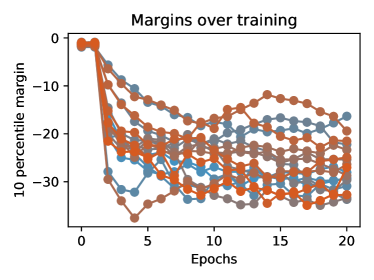
and $C$ is some complexity term. First, note that this construction requires the margin $\gamma$ to be positive. Moreover, the training margin loss is an increasing function of $\gamma$, while the complexity term $C/\gamma$ is decreasing in $\gamma$, thus the conventional way of using the margin bound is to optimize over the margin to balance two terms in the margin bound (Bartlett et al., 2017), rather than pre-specifying the value of the margin dependent on the data. However, we choose to follow the related papers Dziugaite et al. (2020); Jiang et al. (2019), and we use the 10th percentile margin as a robust estimate of the minimum margin in the dataset. We use this margin in all of the margin-normalized generalization metrics. However, in all of the experiments on machine translation, the 10th percentile margin remains negative throughout the whole training, violating the requirement that the bound is evaluated at a positive value of margin. See Figure 12. This problem results from the large Alphabet for machine translation, which makes it difficult to fully interpolate the data, and hence makes the margin-normalized generalization metrics in Dziugaite et al. (2020); Jiang et al. (2019) hard to be applicable to the present setting.

Figure 12: The margins remain negative in the experiments on machine translation due to the large alphabet size.

Appendix D Fitting regression lines using orthogonal distance regression

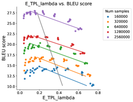
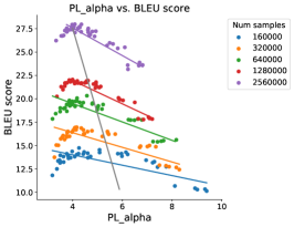
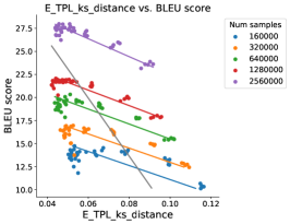
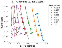
In this section, we fit the regression plots from Figure 5 to 6 using the orthogonal distance regression (Boggs and Rogers, 1990). See Figure 13 to Figure 14.

Figure 13: BLEU-score versus shape metrics. (First row). Trained models grouped by the learning rate. (Second row). Trained models grouped by the number of samples. The regression lines are fitted using orthogonal distance regression.

Figure 14: BLEU-score versus scale metrics. (First row). Trained models grouped by the learning rate. (Second row). Trained models grouped by the number of samples. The regression lines are fitted using orthogonal distance regression.

Appendix E Corroborating results

In this subsection, we consider corroborating results, extending the setup of the main paper to more datasets and different evaluation methods.

E.1 Additional results on natural language processing tasks

We consider three other NLP tasks:

• Roberta (Liu et al., 2019) trained on the masked language modeling task using the Wikitext-103 dataset, and then finetuned on the MNLI dataset (Williams et al., 2018).

• Six-layer base Transformers trained on the language modeling task using the Wikitext-103 dataset (Merity et al., 2016);

• Six-layer base Transformers trained on the next-word prediction task using the Reddit dataset,following the implementation in Bagdasaryan et al. (2020);

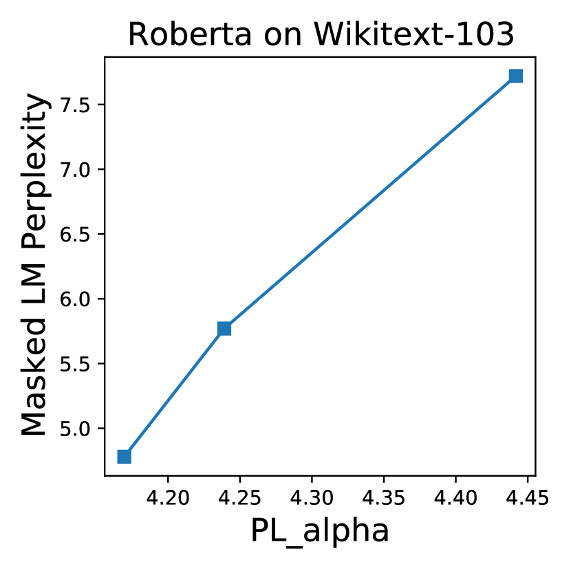
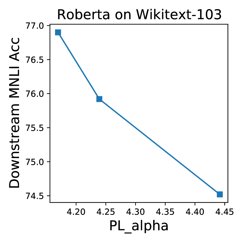
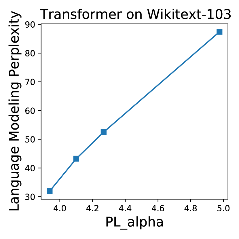
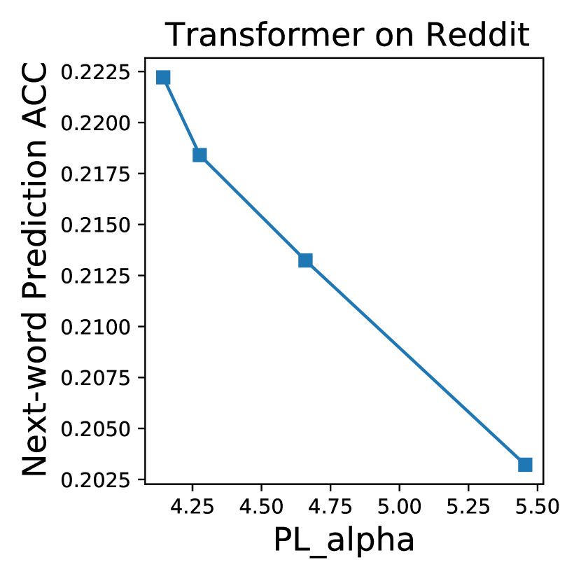
For each task, we train models on different data sizes. Then, we measure the PL_alpha metric and report the correlation with the ground-truth quality metric. See Figure 15. In these experiments, the PL_alpha metric predicts the correct trend, i.e., a lower value of PL_alpha corresponds to a better model.

(a) Lower perplexity is better.

(b) Higher accuracy is better.

(c) Lower perplexity is better.

(d) Higher accuracy is better.

Figure 15: Multiple language processing tasks evaluated using the PL_alpha metric on models trained with different data sizes. The PL_alpha metric correctly predicts the trend in all tasks.

E.2 Evaluating rank correlations using Kendall’s tau metric

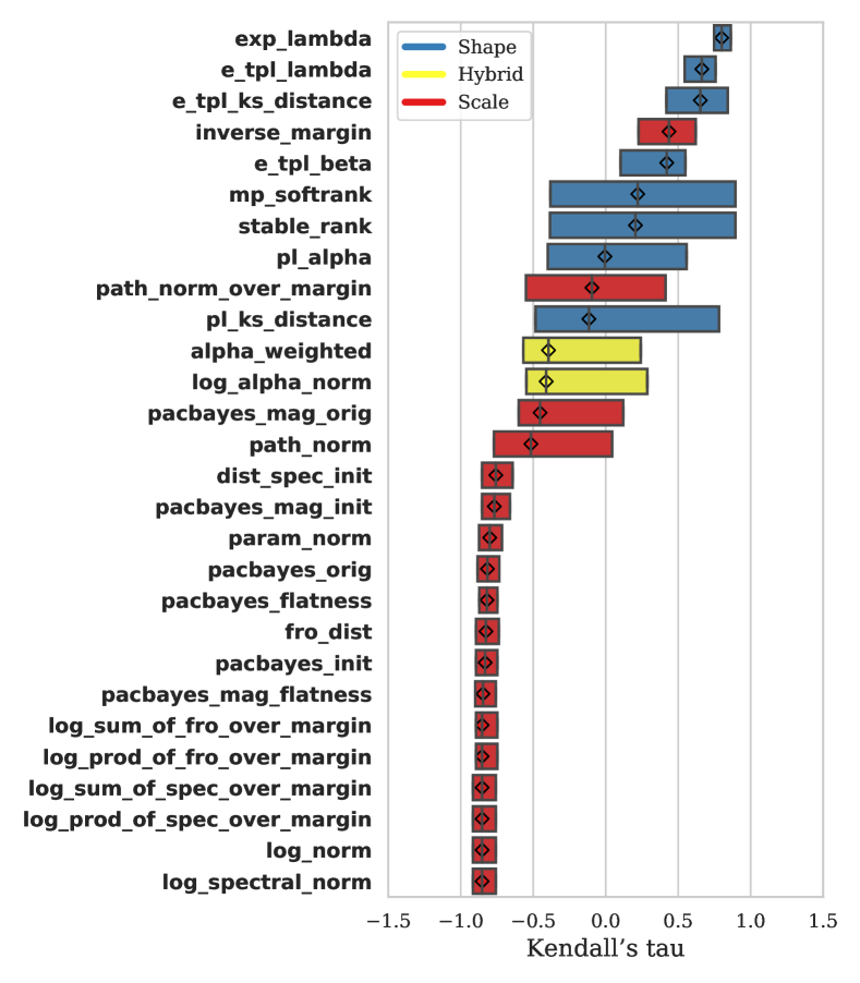
Next, we reimplement Task two using Kendall’s tau to calculate the rank correlations. The results in Figure 16 are very similar to those in Figure 4.

Correlations with model quality

(a) Correlations with model quality. Kendall’s tau between various generalization metrics and BLEU.

Correlations with generalization gap

(b) Correlations with generalization gap. Kendall’s tau between various generalization metrics and the generalization gap.

Figure 16: Evaluating Task Two using Kendall’s tau. Results are similar to those in Figure 4.

References

- (1)
- Alstott et al. (2014) Jeff Alstott, Ed Bullmore, and Dietmar Plenz. 2014. Powerlaw: a Python package for analysis of heavy-tailed distributions. PloS one 9, 1 (2014), e85777.
- Bagdasaryan et al. (2020) Eugene Bagdasaryan, Andreas Veit, Yiqing Hua, Deborah Estrin, and Vitaly Shmatikov. 2020. How to backdoor federated learning. In International Conference on Artificial Intelligence and Statistics. 2938–2948.
- Bartlett et al. (2017) Peter Bartlett, Dylan Foster, and Matus Telgarsky. 2017. Spectrally-normalized margin bounds for neural networks. Advances in Neural Information Processing Systems 30 (2017), 6241–6250.
- Boggs and Rogers (1990) Paul T Boggs and Janet E Rogers. 1990. Orthogonal distance regression. Contemp. Math. 112 (1990), 183–194.
- Bojar et al. (2014) Ondřej Bojar, Christian Buck, Christian Federmann, Barry Haddow, Philipp Koehn, Johannes Leveling, Christof Monz, Pavel Pecina, Matt Post, Herve Saint-Amand, et al. 2014. Findings of the 2014 workshop on statistical machine translation. In Proceedings of the ninth workshop on statistical machine translation. 12–58.
- Chen et al. (2020) Wuyang Chen, Xinyu Gong, and Zhangyang Wang. 2020. Neural Architecture Search on ImageNet in Four GPU Hours: A Theoretically Inspired Perspective. In International Conference on Learning Representations.
- Clauset et al. (2009) Aaron Clauset, Cosma Rohilla Shalizi, and Mark EJ Newman. 2009. Power-law distributions in empirical data. SIAM review 51, 4 (2009), 661–703.
- Dai et al. (2020) Zihang Dai, Guokun Lai, Yiming Yang, and Quoc Le. 2020. Funnel-transformer: Filtering out sequential redundancy for efficient language processing. Advances in neural information processing systems 33 (2020), 4271–4282.
- Dong et al. (2019) Zhen Dong, Zhewei Yao, Amir Gholami, Michael W Mahoney, and Kurt Keutzer. 2019. HAWQ: Hessian aware quantization of neural networks with mixed-precision. In IEEE/CVF International Conference on Computer Vision. 293–302.
- Dziugaite et al. (2020) Gintare Karolina Dziugaite, Alexandre Drouin, Brady Neal, Nitarshan Rajkumar, Ethan Caballero, Linbo Wang, Ioannis Mitliagkas, and Daniel M Roy. 2020. In search of robust measures of generalization. Advances in Neural Information Processing Systems 33 (2020).
- Edunov et al. (2018) Sergey Edunov, Myle Ott, Michael Auli, and David Grangier. 2018. Understanding Back-Translation at Scale. In Proceedings of the 2018 Conference on Empirical Methods in Natural Language Processing. 489–500.
- Elsayed et al. (2018) Gamaleldin Elsayed, Dilip Krishnan, Hossein Mobahi, Kevin Regan, and Samy Bengio. 2018. Large Margin Deep Networks for Classification. Advances in Neural Information Processing Systems 31 (2018), 842–852.
- Feldman (2020) Vitaly Feldman. 2020. Does learning require memorization? a short tale about a long tail. In Proceedings of the 52nd Annual ACM SIGACT Symposium on Theory of Computing. 954–959.
- Foret et al. (2020) Pierre Foret, Ariel Kleiner, Hossein Mobahi, and Behnam Neyshabur. 2020. Sharpness-aware Minimization for Efficiently Improving Generalization. In International Conference on Learning Representations.
- Fort et al. (2019) Stanislav Fort, Huiyi Hu, and Balaji Lakshminarayanan. 2019. Deep ensembles: A loss landscape perspective. Technical Report Preprint: arXiv:1912.02757.
- Garipov et al. (2018) Timur Garipov, Pavel Izmailov, Dmitrii Podoprikhin, Dmitry Vetrov, and Andrew Gordon Wilson. 2018. Loss surfaces, mode connectivity, and fast ensembling of DNNs. In Conference on Neural Information Processing Systems. 8803–8812.
- Izmailov et al. (2018) P Izmailov, AG Wilson, D Podoprikhin, D Vetrov, and T Garipov. 2018. Averaging weights leads to wider optima and better generalization. In Conference on Uncertainty in Artificial Intelligence. 876–885.
- Jiang et al. (2020) Yiding Jiang, Pierre Foret, Scott Yak, Daniel M Roy, Hossein Mobahi, Gintare Karolina Dziugaite, Samy Bengio, Suriya Gunasekar, Isabelle Guyon, and Behnam Neyshabur. 2020. Neurips 2020 competition: Predicting generalization in deep learning. arXiv preprint arXiv:2012.07976 (2020).
- Jiang et al. (2018) Yiding Jiang, Dilip Krishnan, Hossein Mobahi, and Samy Bengio. 2018. Predicting the Generalization Gap in Deep Networks with Margin Distributions. In International Conference on Learning Representations.
- Jiang et al. (2019) Yiding Jiang, Behnam Neyshabur, Hossein Mobahi, Dilip Krishnan, and Samy Bengio. 2019. Fantastic Generalization Measures and Where to Find Them. In International Conference on Learning Representations.
- Kenton and Toutanova (2019) Jacob Devlin Ming-Wei Chang Kenton and Lee Kristina Toutanova. 2019. BERT: Pre-training of Deep Bidirectional Transformers for Language Understanding. In Proceedings of the Annual Conference of the North American Chapter of the Association for Computational Linguistics: Human Language Technologies. 4171–4186.
- Lan et al. (2019) Zhenzhong Lan, Mingda Chen, Sebastian Goodman, Kevin Gimpel, Piyush Sharma, and Radu Soricut. 2019. ALBERT: A lite BERT for self-supervised learning of language representations. In International Conference on Learning Representations.
- Le et al. (2020) Hang Le, Loïc Vial, Jibril Frej, Vincent Segonne, Maximin Coavoux, Benjamin Lecouteux, Alexandre Allauzen, Benoit Crabbé, Laurent Besacier, and Didier Schwab. 2020. FlauBERT: Unsupervised Language Model Pre-training for French. In Proceedings of the 12th Language Resources and Evaluation Conference. 2479–2490.
- Li (2017) Hang Li. 2017. Deep learning for natural language processing: advantages and challenges. National Science Review (2017).
- Liu et al. (2020) Liyuan Liu, Xiaodong Liu, Jianfeng Gao, Weizhu Chen, and Jiawei Han. 2020. Understanding the difficulty of training transformers. arXiv preprint arXiv:2004.08249 (2020).
- Liu et al. (2019) Yinhan Liu, Myle Ott, Naman Goyal, Jingfei Du, Mandar Joshi, Danqi Chen, Omer Levy, Mike Lewis, Luke Zettlemoyer, and Veselin Stoyanov. 2019. Roberta: A robustly optimized BERT pretraining approach. Technical Report Preprint: arXiv:1907.11692.
- Martin and Mahoney (2017) Charles H Martin and Michael W Mahoney. 2017. Rethinking generalization requires revisiting old ideas: statistical mechanics approaches and complex learning behavior. Technical Report Preprint: arXiv:1710.09553.
- Martin and Mahoney (2019) Charles H Martin and Michael W Mahoney. 2019. Traditional and heavy tailed self regularization in neural network models. In International Conference on Machine Learning. 4284–4293.
- Martin and Mahoney (2020) Charles H Martin and Michael W Mahoney. 2020. Heavy-tailed Universality predicts trends in test accuracies for very large pre-trained deep neural networks. In SIAM International Conference on Data Mining. SIAM, 505–513.
- Martin and Mahoney (2021a) Charles H Martin and Michael W Mahoney. 2021a. Implicit Self-Regularization in Deep Neural Networks: Evidence from Random Matrix Theory and Implications for Learning. Journal of Machine Learning Research 22, 165 (2021), 1–73.
- Martin and Mahoney (2021b) Charles H Martin and Michael W Mahoney. 2021b. Post-mortem on a deep learning contest: a Simpson’s paradox and the complementary roles of scale metrics versus shape metrics. Technical Report Preprint: arXiv:2106.00734.
- Martin et al. (2021) Charles H Martin, Tongsu Serena Peng, and Michael W Mahoney. 2021. Predicting trends in the quality of state-of-the-art neural networks without access to training or testing data. Nature Communications 12, 1 (2021), 1–13.
- McAllester (1999) David A McAllester. 1999. PAC-Bayesian model averaging. In Annual Conference on Computational Learning Theory. 164–170.
- Merity et al. (2016) Stephen Merity, Caiming Xiong, James Bradbury, and Richard Socher. 2016. Pointer sentinel mixture models. Technical Report Preprint: arXiv:1609.07843.
- Nagarajan and Kolter (2019) Vaishnavh Nagarajan and J Zico Kolter. 2019. Uniform convergence may be unable to explain generalization in deep learning. Advances in Neural Information Processing Systems 32 (2019).
- Nakkiran et al. (2019) Preetum Nakkiran, Gal Kaplun, Yamini Bansal, Tristan Yang, Boaz Barak, and Ilya Sutskever. 2019. Deep Double Descent: Where Bigger Models and More Data Hurt. In International Conference on Learning Representations.
- Neyshabur et al. (2017) Behnam Neyshabur, Srinadh Bhojanapalli, David Mcallester, and Nati Srebro. 2017. Exploring Generalization in Deep Learning. Advances in Neural Information Processing Systems 30 (2017), 5947–5956.
- Neyshabur et al. (2018) Behnam Neyshabur, Srinadh Bhojanapalli, and Nathan Srebro. 2018. A PAC-Bayesian Approach to Spectrally-Normalized Margin Bounds for Neural Networks. In International Conference on Learning Representations.
- Neyshabur et al. (2015) Behnam Neyshabur, Ryota Tomioka, and Nathan Srebro. 2015. Norm-based capacity control in neural networks. In Conference on Learning Theory. PMLR, 1376–1401.
- Ott et al. (2018) Myle Ott, Sergey Edunov, David Grangier, and Michael Auli. 2018. Scaling Neural Machine Translation. In Proceedings of the Third Conference on Machine Translation: Research Papers. 1–9.
- Papineni et al. (2002) Kishore Papineni, Salim Roukos, Todd Ward, and Wei-Jing Zhu. 2002. BLEU: a method for automatic evaluation of machine translation. In Proceedings of the 40th annual meeting of the Association for Computational Linguistics. 311–318.
- Pitas et al. (2017) Konstantinos Pitas, Mike Davies, and Pierre Vandergheynst. 2017. Pac-bayesian margin bounds for convolutional neural networks. Technical Report Preprint: arXiv:1801.00171.
- Radford et al. (2019) Alec Radford, Jeffrey Wu, Rewon Child, David Luan, Dario Amodei, Ilya Sutskever, et al. 2019. Language models are unsupervised multitask learners. OpenAI blog 1, 8 (2019), 9.
- Raffel et al. (2020) Colin Raffel, Noam Shazeer, Adam Roberts, Katherine Lee, Sharan Narang, Michael Matena, Yanqi Zhou, Wei Li, Peter J Liu, et al. 2020. Exploring the limits of transfer learning with a unified text-to-text transformer. Journal of Machine Learning Research 21, 140 (2020), 1–67.
- Shen et al. (2020) Dinghan Shen, Mingzhi Zheng, Yelong Shen, Yanru Qu, and Weizhu Chen. 2020. A simple but tough-to-beat data augmentation approach for natural language understanding and generation. Technical Report Preprint: arXiv:2009.13818.
- Tanay and Griffin (2016) Thomas Tanay and Lewis Griffin. 2016. A boundary tilting persepective on the phenomenon of adversarial examples. Technical Report Preprint: arXiv:1608.07690.
- Turc et al. (2019) Iulia Turc, Ming-Wei Chang, Kenton Lee, and Kristina Toutanova. 2019. Well-read students learn better: On the importance of pre-training compact models. Technical Report Preprint: arXiv:1908.08962.
- Vaswani et al. (2017) Ashish Vaswani, Noam Shazeer, Niki Parmar, Jakob Uszkoreit, Llion Jones, Aidan N Gomez, Łukasz Kaiser, and Illia Polosukhin. 2017. Attention is all you need. In Advances in neural information processing systems. 5998–6008.
- Wei and Ma (2019) Colin Wei and Tengyu Ma. 2019. Improved sample complexities for deep neural networks and robust classification via an all-layer margin. In International Conference on Learning Representations.
- Williams et al. (2018) Adina Williams, Nikita Nangia, and Samuel Bowman. 2018. A Broad-Coverage Challenge Corpus for Sentence Understanding through Inference. In Proceedings of the 2018 Conference of the North American Chapter of the Association for Computational Linguistics: Human Language Technologies, Volume 1 (Long Papers). 1112–1122.
- Wolf et al. (2020) Thomas Wolf, Lysandre Debut, Victor Sanh, Julien Chaumond, Clement Delangue, Anthony Moi, Pierric Cistac, Tim Rault, Rémi Louf, Morgan Funtowicz, Joe Davison, Sam Shleifer, Patrick von Platen, Clara Ma, Yacine Jernite, Julien Plu, Canwen Xu, Teven Le Scao, Sylvain Gugger, Mariama Drame, Quentin Lhoest, and Alexander M. Rush. 2020. Transformers: State-of-the-Art Natural Language Processing. In Proceedings of the 2020 Conference on Empirical Methods in Natural Language Processing: System Demonstrations. Association for Computational Linguistics, 38–45.
- Xiong et al. (2020) Ruibin Xiong, Yunchang Yang, Di He, Kai Zheng, Shuxin Zheng, Chen Xing, Huishuai Zhang, Yanyan Lan, Liwei Wang, and Tieyan Liu. 2020. On layer normalization in the transformer architecture. In International Conference on Machine Learning. PMLR, 10524–10533.
- Yang et al. (2021) Yaoqing Yang, Liam Hodgkinson, Ryan Theisen, Joe Zou, Joseph E Gonzalez, Kannan Ramchandran, and Michael W Mahoney. 2021. Taxonomizing local versus global structure in neural network loss landscapes. In Thirty-Fifth Conference on Neural Information Processing Systems.
- Yang et al. (2020) Yaoqing Yang, Rajiv Khanna, Yaodong Yu, Amir Gholami, Kurt Keutzer, Joseph E Gonzalez, Kannan Ramchandran, and Michael W Mahoney. 2020. Boundary thickness and robustness in learning models. Advances in Neural Information Processing Systems 33 (2020).
- Yang et al. (2023) Yaoqing Yang, Ryan Theisen, Liam Hodgkinson, Joseph E Gonzalez, Kannan Ramchandran, Charles H Martin, and Michael W Mahoney. 2023. Test accuracy vs. generalization gap: model selection in NLP without accessing training or testing data. In proceedings of the 29th ACM SIGKDD international conference on knowledge discovery & data mining.
- Yuan et al. (2021) Weizhe Yuan, Graham Neubig, and Pengfei Liu. 2021. Bartscore: Evaluating generated text as text generation. Advances in Neural Information Processing Systems 34 (2021), 27263–27277.
- Zhang et al. (2019) Tianyi Zhang, Varsha Kishore, Felix Wu, Kilian Q Weinberger, and Yoav Artzi. 2019. BERTScore: Evaluating Text Generation with BERT. In International Conference on Learning Representations.
- Zhang et al. (2020) Yizhe Zhang, Siqi Sun, Michel Galley, Yen-Chun Chen, Chris Brockett, Xiang Gao, Jianfeng Gao, Jingjing Liu, and William B Dolan. 2020. DIALOGPT: Large-Scale Generative Pre-training for Conversational Response Generation. In Proceedings of the 58th Annual Meeting of the Association for Computational Linguistics: System Demonstrations. 270–278.