A semi-empirical analysis of the paramagnetic susceptibility of solid state magnetic clusters

Abstract

Recent developments in the synthesis of new magnetic materials lead to the discovery of new quantum paramagnets. Many of these materials, such as the perovskites Ba₄LnMn₄O₁₂ (Ln = Sc or Nb), Ba₃Mn₂O₈, and Sr₃Cr₂O₈ present isolated magnetic clusters with strong intracluster interactions but weak intercluster interactions, which delays the onset of order to lower temperatures ($T$). This offset between the local energy scale and the magnetic ordering temperature is the hallmark of magnetic frustration. At sufficient high-$T$, the paramagnetic susceptibility ($\chi$) of frustrated cluster magnets can be fit to a Curie-Weiss law, but the derived microscopic parameters cannot in general be reconciled with those obtained from other methods. In this work, we present an analytical microscopic theory to obtain $\chi$ of dimer and trimer cluster magnets, the two most commonly found in literature, making use of suitable Heisenberg-type Hamiltonians. We also add intercluster interactions in a mean-field level, thus obtaining an expression to the critical temperature of the system and defining a new effective frustration parameter $f_{\text{eff}}$. Our method is exemplified by treating the $\chi$ data of some selected materials.

I Introduction

The magnetism of solids encompass a really broad research field, ranging from studies of magnets for applications to the investigation of the fundamentals of electronic interactions in matter [1, 2]. Energy scales of the magnetic interactions are set by the exchange constants $J$, which are mainly determined by the nature of the interacting spins and the electronic structure of the magnetic active atom coordination structure [3].

To estimate $J$ is an important step towards understanding the magnetism of a particular material. The first approach to this problem is given by the Curie-Weiss analysis of the material paramagnetic susceptibility $\chi$. For the vast majority of magnetic solid state materials, $\chi$ as a function of temperature ($T$) is fairly described by the Curie-Weiss expression (Equation 1)

$$\chi(T)=\frac{C}{T-\theta_{\text{CW}}}$$ (1)

where $C$ and $\theta_{\text{CW}}$ are the Curie and Curie-Weiss constants, respectively. As is well known, $\theta_{\text{CW}}$ can be connected to $J$ and, in a mean field approach, to the magnetic ordering temperature of solids [2], whereas the value of $C$ relates to the single ion spin configuration in the solid. Exceptions, however, do exist for which the Curie-Weiss approach cannot provide a physically meaningful set of parameters. Recently, the magnetic properties of a large class of perovskite-type materials were reviewed [4] providing many important examples where the set of the obtained $C$ and $\theta_{\text{CW}}$ parameters do not connect well with the known properties of the materials. This happens in respective of the apparent good fittings of the high-$T$ $\chi$ data to the Curie-Weiss expression (Eq. 1). Illustrative examples are provided by Ba₄$Ln$Mn₃O₁₂ ($Ln=$ Sc or Nb) $\chi$ data [5, 6], for which the obtained $C$ values are much too low to be compared with the expectation of $S=2$ spins from Mn³⁺ cations. If the obtained $C$ values are not reliable, it also raises questions about the obtained $\theta_{\text{CW}}$ parameters.

The Ba₄$Ln$Mn₃O₁₂ ($Ln=$ Sc or Nb) materials shared the same crystal structure (see Figure 1) which host as building blocks isolated clusters of magnetic cations, sitting within face sharing Oxygen octahedra. This building block displays a large number of exchange paths which in turn contribute to large $J$’s [3]. The local (within the cluster) magnetic interactions are strong but the interclusters interactions are weak, since the clusters are well separated in the structure. The onset of order, if observed, is thus delayed to low temperatures. This is the hallmark of frustrated magnetism [7].

A feature of frustrated magnetism is that if the frustration is strong enough, it may compete with quantum fluctuations for the system ground state, giving rise to exotic types of quantum magnetism, such as quantum spin liquids [8, 9] or Bose-Einstein condensates of spin excitations [10, 11]. Thus, materials hosting this type of building blocks are good platforms to search for exotic magnetism as noted in Ref. [4]. The usual way to quantify frustration is by determining the frustration parameter $f$, or a lower bound to $f$, which requires a trustworthy determination of the system’s energy scales.

In this work, we propose to analyze the paramagnetic data of materials hosting magnetic clusters adopting Heisenberg-type Hamiltonians [2] parametrized by exchange constants $J_{n}$ , with the intercluster interactions taken into account by a mean field approach. This is an alternative, semi-empirical approach which, while already tested in the case of spin dimers [12, 13], is not particularly explored in the case of spin trimers [5, 6].

In section II, we provide a general perspective on the proposed methodology and then we illustrate our approach by fitting the $\chi$ data of a series of materials hosting magnetic clusters in section III. Finally, we move to discuss and summarize our results. Most interesting, we define a new frustration parameter $f_{\text{eff}}$ in terms of the energy scale of the effective intercluster interactions. In doing so, we show some frustrated magnets are unlikely to display quantum many body states at further lower temperatures, while other remain as strong candidates to host this type of Physics.

II Models

Our approach is mainly intended to the description of the magnetic properties of solids hosting magnetic clusters as exemplified by the crystal structures in Figure 1$(a)\text{, }(d)\text{, }(f)\text{ and }(i)$. In all cases, the magnetic cations are connected by multiple exchange paths, causing the local magnetic interaction to be strong. We thus treat single cluster magnetic properties by means of a microscopic Heisenberg-type Hamiltonian:

$$\mathcal{H}=\sum_{ij}J_{ij}\boldsymbol{S}_{i}\cdot\boldsymbol{S}_{j}$$ (2)

where the indexes $i$ and $j$ run within the cluster sites, $\boldsymbol{S}_{i}$ are the spin operators of the magnetic cations and $J_{ij}$ is the exchange constant between spins $i$ and $j$. For instance, applied to the case of the magnetic trimers, Equation 2 reads:

$$\mathcal{H}_{\text{trim}}=J_{12}S_{1}\cdot S_{2}+J_{23}S_{2}\cdot S_{3}+J_{13}S_{1}\cdot S_{3}.$$ (3)

In this work, we shall also illustrate our approach with magnetic dimers, that can be described by:

$$\mathcal{H}_{\text{dim}}=J_{1}S_{1}\cdot S_{2}.$$ (4)

Once the proper Hamiltonian is determined, we consider a weak magnetic field $H$ and evaluate the system energy levels up to first order in the field:

$$E_{n}=E_{n}^{(0)}+HE_{n}^{(1)}+\mathcal{O}(2)$$ (5)

and the results are applied to calculate the system magnetic bare susceptibility in the usual units of $\text{emu}\cdot\text{mol}^{-1}\cdot\text{Oe}^{-1}$.

$$\bar{\chi}(\beta)=N_{A}k_{B}\mu_{B}^{2}\frac{\sum_{n}e^{-E_{n}^{(0)}\beta}\left(E_{n}^{(1)}/\mu_{B}\right)^{2}}{\sum_{n}e^{-E_{n}^{(0)}\beta}}\beta$$ (6)

where $N_{A}$ is the Avogadro number, $k_{\text{B}}$ is the Boltzmann constant, $\mu_{\text{B}}$ is the Bohr magneton, $\beta=1/k_{B}T$ and $E_{n}^{(0)}$and $E_{n}^{(1)}$ are, respectively, the zeroth and first order eigenvalues of $\mathcal{H}$ (Equation 2) as defined by Equation 5. In many situations of interest, Equations 3 and 4 can be diagonalized analytically (see appendix A) and thus the perturbation theory to write down $\bar{\chi}$ can be carried out straightforwardly.

The expression obtained from Equation 6 contains the $J_{n}$ constants as free parameters. The next step is to treat the cluster-cluster interaction in a mean field approximation:

$$\chi=\frac{\bar{\chi}}{1-\lambda\bar{\chi}}$$ (7)

where $\lambda$ is the molecular field parameter, describing the inter-cluster interaction. As we shall discuss, in many instances it is $\lambda$ which should be adopted to estimate the values of the frustration parameter $f$.

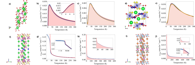
Figure 1: $(a)$ Structural model of the Ba₃Mn₂O₈ and Sr₃Cr₂O₈ materials (symmetry group R$\bar{3}$m). The spheres represent Mn/Cr (purple; magnetic), Ba (green), and O (red) atoms. $(b)$ Ba₃Mn₂O₈ $\chi$ data (blue dots) and theoretical fit (red line) $(c)$ Sr₃Cr₂O₈ $\chi$ data with blue as yellow dots representing, respectively, data obtained with the field applied parallel and perpendicular to the sample’s $ab$ plane. The red and black lines represent the respective theoretical fittings. $(d)$ Sr₃Co₃S₂O₃ structural model. The spheres represent Co (blue; magnetic), Sr (green), O (red), and S (yellow) atoms. $(e)$ As in $(c)$ but for the Sr₃Co₃S₂O₃ material. $(f)$ Structural model of the Ba₄ScMn₃O₁₂ and Ba₄NbMn₃O₁₂ materials (symmetry group R$3$m). The spheres represent Mn (purple/yellow; magnetic), Ba (green), O (red), and Nb/Sc (blue) atoms. $(g)-(h)$ Susceptibility data (blue dots) and respective fitting (red line) for the Ba₄ScMn₃O₁₂, and Ba₄NbMn₃O₁₂ materials, respectively. $(i)$ Structural model of BaTi_0.5Mn_0.5O₃. The spheres represent Mn (purple; magnetic), Ti (light blue), O (red), and Ba (orange) atoms. $(j)$ Susceptibility data (blue dots) and fittings (red line) for BaTi_0.5Mn_0.5O₃.

III Results

Now that we have developed the appropriate tools to model clusters, the next step is to apply the theory to better understand some model systems. We start taking spin dimers into account, as a way to illustrate our approach in an already familiar environment, and then we move to investigate spin trimers in some selected hexagonal perovskites [4]. These low symmetry systems are prone to exhibit rotated Oxygen octahedra coordinating transition metal cations, which will precisely give rise to the multiplicity of the exchange paths that cause the formation of strongly coupled magnetic clusters. We end this section analyzing a system exhibiting both spin dimers and spin trimers.

III.1 Dimers

We select the Ba₃Mn₂O₈ [14, 15, 16], Sr₃Cr₂O₈ [11], and Sr₃Co₃S₂O₃ [17] spin dimer materials to our analysis. The same trigonal structure, described by the space group R$\bar{3}$m, are shared by the two former materials and is depicted in Figure 1$(a)$. The Sr₃Co₃S₂O₃ structure is described by the space group Pbam and is presented in Figure 1$(d)$.

Focusing on the trigonal materials, charge balance in the systems dictate that we have Mn⁵⁺and Cr⁵⁺ cations which carry, respectively, $S=1$ and $S=1/2$ spins. The Ba₃Mn₂O₈ total $\chi$ is modeled by adopting one exchange constant $J_{1}$ and one $\lambda$ molecular field parameter plus a constant diamagnetic contribution $\chi_{0}$ as in Equation 8:

$$\chi(T)=q_{\text{dim}}\chi_{\text{dim}}+\chi_{0}$$ (8)

where $q_{\text{dim}}$ is the molar fraction of the dimer specimen in the sample and $\chi_{\text{dim}}$ is obtained from 7 (with $\bar{\chi}$ as suitable to case of dimers, see Equation 13) and carries the $J_{1}$ and $\lambda$ parameters. The fitting and experimental data are presented in Figure 1$(b)$ and the obtained parameters are $J_{1}/k_{B}=17.66(7)$ K and $\lambda=-16.35(9)$ Oe$\cdot$mol$\cdot$emu^-1.

In the case of the Sr₃Cr₂O₈ material [11], we model to Equation 8 an orphan spin contribution ($C/T$) to account for the observed rise in $\chi$ at low temperatures. The fitting and experimental data are presented in Figure 1$(c)$ and the obtained parameters are $J_{1}/k_{B}=61.5(2)$ K, $\lambda=-5(1)$ Oe$\cdot$mol$\cdot$emu^-1, $C=4.06(9)\cdot 10^{-3}$ emu$\cdot$K/mol, and $\chi_{0}=1.9(1)\cdot 10^{-4}$ emu/mol Cr.

Lastly, as discussed in Ref. [17], the Sr₃Co₃S₂O₃ compound was expected to hold an effective spin $S=3/2$ because of the Co²⁺ valence, which is again deduced from charge balance. Due to the octahedral crystal field, however, Co²⁺ cations carry low $S=1/2$ spins. The total $\chi$ is modeled by Equation 8 and the obtained parameters for the FC (ZFC) susceptibility data are $J_{1}/k_{B}=97.9(2)$ K ($J_{1}/k_{B}=99.6(2)$ K), $\lambda=2.50(16)$ Oe$\cdot$mol$\cdot$emu^-1 ($\lambda=0.94(11)$ Oe$\cdot$mol$\cdot$emu^-1), and $\chi_{0}=0.00829(3)$ emu/mol Co ($\chi_{0}=0.00824(3)$ emu/mol Co).Slightly distinct values are reported in Ref. [17] because here we included the intercluster interactions, which we found to be ferromagnetic ($\lambda>0$). The fitting and experimental data are presented in Figure 1$(e)$.

III.2 Trimers

Two materials presenting magnetic trimers were selected: Ba₄ScMn₃O₁₂ and Ba₄NbMn₃O₁₂. The materials share the same crystal structure which is depicted in Figure 1$(f)$. In both cases, we assume the presence of Mn⁴⁺cations carrying $S=3/2$ spins and Hamiltonian 3 is adopted to describe the trimer magnetism. It should be clear, however, that we can adopt $J_{12}=J_{23}=J_{1}$ and $J_{13}=J_{2}=\alpha J_{1}$, where $0\leq\alpha\leq 1$. This assumption make it possible to perform an exact diagonalization of 3. In principle, one could think of $\alpha$ as a small number, but the large multiplicity of exchange paths cause $\alpha$ to be $>0.5$ for magnetic cations within face sharing octahedra. Intertrimer interactions are described by just one molecular field parameter $\lambda$. We adopt the model susceptibility:

$$\chi(T)=q_{\text{trim}}\chi_{\text{trim}}+\chi_{0}$$ (9)

where $q_{\text{trim}}$ is the molar fraction of the trimer specimen in the sample and $\chi_{\text{trim}}$ is obtained from equation 9 (see Equation 15 for more details). One should note that $\chi_{\text{trim}}$ carries three parameters: the exchange constants $J_{1}$ and $J_{2}$ and $\lambda$.

In the case of Ba₄ScMn₃O₁₂, the following parameters are obtained: $J_{1}/k_{B}=199.44(2)$ K, $\alpha=0.60041(1)$, $\chi_{0}=-2.67(4)\cdot 10^{-5}$ emu$\cdot$K/mol/Oe, and a negligible value of $\lambda$. As for Ba₄NbMn₃O₁₂ , we obtain: $J_{1}/k_{B}=172(1)\text{ K}$, $\alpha=0.7651(1)$, $\lambda=77.4(5)$ mol$\cdot$Oe/emu/K, and $\chi_{0}=-0.00263(3)$ emu$\cdot$K/mol/Oe. The fittings results are compared to the data in Figure 1$(f)-(g)$, respectively. The significant value of $\lambda$ found in the later case is in agreement with the observed critical temperature of $\approx 32$ K determined for Ba₄NbMn₃O₁₂.

III.3 Dimers and trimers

We now turn to the challenging case offered by the BaTi_0.5Mn_0.5O₃ [18, 19] material, which presents spin dimers, trimers, and orphans. Its crystal structure is depicted in Figure 1$(i)$. The proposed model to $\chi$ assumes the following form:

$$\chi(T)=q_{\text{trim}}\chi_{\text{trim}}+q_{\text{dim}}\chi_{\text{dim}}+q_{\text{orp}}\chi_{\text{orp}}+\chi_{0}$$ (10)

where $q_{\text{orp}}$ is the molar fraction of the orphan spins in the sample and $\chi_{\text{orp}}$ is the orphan spin susceptibility. As discussed elsewhere [18, 19], the fractions are statistically determined to be: $q_{\text{trim}}=q_{\text{orp}}=1/16$, and $q_{\text{dim}}=2/16$. We adopt a Curie-Weiss form to $\chi_{\text{orp }}$ (with $C_{\text{orp}}$ and $\theta_{\text{orp}}$ parameters). The obtained fitting is compared to the data in Figure 1$(j)$ and the obtained cluster parameters are: $J_{1}/k_{B}=201(2)$ K, $\alpha=0.85(2)$, and $\lambda=48(15)$ mol$\cdot$Oe/emu/K (calculated considering only timer-trimer interactions), while the orphan spin parameters are: $\theta_{\text{orp}}=14.4(5)$ K and $C_{\text{orp}}=0.217(2)$ emu$\cdot$K/mol/Oe.

Table 1: Summary of experimentally obtained parameters within our model paramagnetic susceptibility.

Material	$J_{1}/k_{B}$ (K)	$\alpha$ ($J_{2}/J_{1}$)	$\lambda$ (Oe$\cdot$mol/emu)	$s_{\text{eff}}$	$T_{\text{C,eff}}$ (K)	$f_{\text{eff}}$	$f_{\text{CW}}$
Ba3Mn2O8	$17.66(7)$	-	$-16.35(9)$	$1$	$16.36(9)$	$9.14$	$18.7$
Sr3Cr2O8	$61.5(2)$	-	$-5(1)$	$1/2$	$1.7(4)$	$0.90$	$26.2$
Sr3Co3S2O3	$99.6(2)$	-	$1.82(17)$	$1/2$	$2.4(2)$	$0.63$	$42.8$
Ba4ScMn3O12	$199.44(2)$	$0.60041(1)$	$-0.05543(5)$	$1/2$	$0.0208(2)$	$0.01$	$0.41$
Ba4NbMn3O12	$172(1)$	$0.7651(1)$	$77.4(5)$	$1/2$	$29.0(1)$	$0.91$	$0.02$
BaTi0.5Mn0.5O3	$201(2)$	$0.85(2)$	$48(15)$	$1/2$	$18(6)$	$180$	$1024$

IV Discussion

We would like to discuss two aspects or our results: $i)$ the set of obtained parameters and $ii)$ the interpretation of $\lambda$ and its relation to the frustration parameter $f$, which is of great relevance to the characterization of putative quantum phases associated to these materials. We start with the later.

By comparing the high temperature ($\beta\rightarrow 0$) limit of Equation 7 to the the Curie-Weiss law (Equation 1), one reaches the expression $\bar{\theta}_{\text{CW}}=\lambda C$, which in turn can be applied to define an effective exchange constant $J_{\text{eff }}$for the intercluster interaction as $\lambda\equiv\frac{J_{\text{eff}}k_{B}}{g^{2}\mu_{B}^{2}N_{A}}$. This expression gives a well defined meaning to $\lambda$ as the parameter describing long range intercluster interactions.

Indeed, in forming the clusters, most of the magnetic degrees of freedom are frozen at low temperatures and the remaining degrees of freedom interact with an energy scale characterized by $\bar{\theta}_{\text{CW}}$. Therefore, the correct estimate to the system frustration should be given by a new effective frustration parameter $f_{\text{eff}}\equiv|\frac{\bar{\theta}_{\text{CW}}}{T_{\text{L}}}|$ where $T_{\text{L}}$ is the lowest temperature at which the system is still in the paramagnetic state. If order is not observed, $T_{\text{L}}$ is given by the lowest experimentally achieved temperature and the $f_{\text{eff}}$ parameter thus obtained is a lower bond to $f_{\text{eff}}$. Moreover, we have now a way to estimate the temperature for long range magnetic order that will be triggered by the intercluster interactions. We shall name this the effective critical temperature, $T_{\text{C,eff}}$. Adopting the overall mean field relation $|\theta_{\text{CW}}|=T_{\text{C }}$, where $T_{\text{C }}$ is the magnetic critical temperature, we write $|\bar{\theta}_{\text{CW}}|=T_{\text{C,eff}}$ and then $|\bar{\theta}_{\text{CW}}|=T_{\text{C,eff}}=\lambda C$. To obtain $C$, we consider that the remaining degrees of freedom of the magnetic clusters should be associated with an effective spin $s_{\text{eff}}$ , thus we can write:

$$T_{\text{C,eff}}=|J_{\text{eff}}|\frac{s_{\text{eff}}(s_{\text{eff}}+1)}{3}$$ (11)

We propose that $s_{\text{eff}}$ should be calculated as either the expectation value of the $S_{z}$ operator of the cluster ground state spin state in the case of trimers, or by the first excited total spin state of the cluster, in the case of dimers. Concerning the later, the necessity of considering the first excited state in the case of dimers can be understood as follows: the first order energy correction for the spin excitation in a given magnetic field $H$ is of the type $E_{0}^{(1)}=-g\mu_{B}Hs_{\text{eff}}$. For an antiferromagnetic dimer, $s_{\text{eff}}$ is always $0$ if one adopts the spin ground state to calculate $s_{\text{eff}}$. Our assumption about $s_{\text{eff}}$ thus means that the system magnetism at low-$T$ is dominated only by the ground state spin configuration except when it turns out be null, when one should peak the first excited state. In the appendix B we show how to determine $s_{\text{eff}}$ for trimers.

All obtained parameters are shown in table 1. We also list $f_{\text{CW}}$ parameters which are the frustration parameters obtained from the usual Curie-Weiss analysis. The values of $J_{n}$ clearly distinguish between the exchange constants due to magnetic interactions mediated by corner sharing octahedra, the case of the selected dimer based materials, and face sharing octahedra, the case of selected trimer based materials. Intercluster interactions of both FM and AFM types are present, but are definitely small energy scales when compared to the intracluster interactions. Notwithstanding, these are the energy scales that will control the onset of magnetic order at sufficient low temperatures.

Comparing $f_{\text{eff}}$ and $f_{\text{CW}}$, one can conclude that all dimer based materials are at most moderately frustrated magnetic systems (the case of Ba₃Mn₂O₈) if the intercluster energy scale is considered. It is therefore unlikely that a quantum magnetic state will emerge from these materials. Interesting glassy behavior, however, could be expected.

The case of the trimer based materials is even more revealing. Ba₄NbMn₃O₁₂ order at $T\approx 32$ K and is not a frustrated material. Ba₄ScMn₃O₁₂, on the other hand, is expected to order only about $T\approx 0.02$ K, a temperature at which quantum effects could tune the system into an exotic ground state. The intercluster interactions, however, are rather weak making it unlikely. The mixed dimer/trimer material BaTi_0.5Mn_0.5O₃ remain characterized as a strongly frustrated magnet with relatively large intercluster interactions. As already observed [19], the system disorder is large, which may hinder the appearance of a quantum spin liquid, although the physics will be that of a correlated disordered quantum magnet. Thus, further investigations at low $T$ are invited.

V Conclusion and perspectives

The Curie-Weiss law has great use to analyze the magnetism of very general systems. It fails, however, in giving a microscopic view of the problem. We found the later to be particularly critical to determine the energy scale of the magnetic interaction of materials hosting magnetic clusters. Therefore, in this work we proposed a methodology to study the susceptibility of cluster magnets which considers intracluster and intercluster interactions.

Our methods were applied to a series of materials and the obtained parameters were discussed and put into perspective. Our semiempirical approach to the problem could identify potential material candidates to low temperature explorations in the search for quantum many body ground states. Our main proposal is that intercluster interactions must be taken into account while discussing the level of frustration in the system. This is the energy scale that correctly sets the odds for a system to display a quantum many body state.

In particular, the trimmer system Ba₄ScMn₃O₁₂, which present a very small inter-cluster interaction, with a predicted ordering temperature of $\approx 0.02$ K, is unlikely to display this type of physics, but the case of mixed dimer/trimmer system BaTi_0.5Mn_0.5O₃ remain open for further experimental investigation.

Lastly, one could argue that our model, in comparison to Curie-Weiss analysis, is only adding fitting parameters. We point out, however, that our approach starts from a microscopic model and then scales to the description of macroscopic susceptibility data. The adopted parameter set are thus not arbitrary. In fact, the present method proposes a more meaningful analysis of magnetic susceptibility data of systems presenting magnetic clusters.

VI Acknowledgments

We thank H. Tanaka and collaborators, A. Aczel and collaborators Aczel et al. [11], K. To Lai and M. Valldor Lai and Valldor [17] and E. Komleva and collaborators Komleva et al. [20] who provided us with the Ba₃Mn₂O₈, Sr₃Cr₂O₈, Sr₃Co₃S₂O₈, and Ba₄NbMn₃O₁₂ data, respectively. The financial support from Fundação de Amparo a Pesquisa do Estado de São Paulo is acknowledged by L.B.B. (Grant No. 2019/27555-9) and F.A.G. (Grant No. 2019/25665-1).

VII Appendix

Appendix A Exact diagonalization

In the following development we present analytical solutions to the problems of dimer and trimer clusters interactions, and also to inter-cluster interactions. Our approach to study interactions consists in find the eigenenergies of the respective Heisenberg Hamiltonian, $\mathcal{H}=\sum_{ij}J_{ij}S_{i}\cdot S_{j}$, in which $S_{i}$ are spin operators and $J_{ij}$ are the exchange constants (usually in units of K), related to the probability of electronic hopping from site $i$ to site $j$.

A.1 Dimers

Let us consider a dimer system consisting of two sites with electrons which may hop to the neighbor and interact effectively with total spins $S_{1}$ and $S_{2}$, and exchange constant $J_{1}$. The Hamiltonian treating the interaction is the Heisenberg Hamiltonian showed in Equation 12.

$$\mathcal{H}_{\text{dim}}=J_{1}S_{1}\cdot S_{2}$$ (12)

The basis which diagonalizes the operators $S_{1}^{2},S_{2}^{2},S_{d}^{2}=(S_{1}+S_{2})^{2}$, and $S_{z}$ (of dimension $(2s_{1}+1)(2s_{2}+1)$) has eigenvectors $|s_{d},m_{d}\rangle$, where $S_{d}^{2}|s_{d},m_{d}\rangle=\hbar s_{d}(s_{d}+1)|s_{d},m_{d}\rangle$, and $S_{z}|s_{d},m_{d}\rangle=\hbar m_{d}|s_{d},m_{d}\rangle$. All expected values in this subsection are taken with respect to these eigenkets.

With this basis, it is possible to diagonalize the Hamiltonian in Equation 12 for any values of spin operators $S_{1}$ and $S_{2}$, and find $E=\langle s_{d},m_{d}|\mathcal{H}|s_{d},m_{d}\rangle=J_{1}\langle S_{1}\cdot S_{2}\rangle$. The trick here is to define a dimer quantum number such that $\langle S_{d}^{2}\rangle=\langle(S_{1}+S_{2})^{2}\rangle=\langle S_{1}^{2}+S_{2}^{2}-2S_{1}\cdot S_{2}\rangle=s_{d}(s_{d}+1)\implies\langle S_{1}\cdot S_{2}\rangle=\frac{1}{2}[s_{d}(s_{d}+1)-s_{1}(s_{1}+1)-s_{2}(s_{2}+1)]$. The quantum number $s_{d}$ runs from $|s_{1}-s_{2}|$ through $s_{1}+s_{2}$ in steps of 1. Therefore, Equation 13 holds for the eigenenergies of the dimer system.

$$E_{d}(s_{d})=\frac{J_{1}}{2}[s_{d}(s_{d}+1)-s_{1}(s_{1}+1)-s_{2}(s_{2}+1)].$$ (13)

Adding a Zeeman-type perturbation $\mathcal{H}_{Z}=-g\mu_{B}HS_{z}$ (in units of $\hbar$) in the z-direction can be done straightforwardly: $E_{n}^{(1)}=-g\mu_{B}Hm_{d}$.

A.2 Trimers

Differently of dimers, the susceptibility of trimers does not goes to zero $T\rightarrow 0$ , because each trimer will still present a net magnetic moment.

Now the Heisenberg Hamiltonian of a trimer cluster is written as in Equation 3. Here, we specialize in the case $J_{12}=J_{23}=J_{1}$ and $J_{13}=J_{2}=\alpha J_{1}$, where $0\leq\alpha\leq 1$, which is adequate for systems of magnetic trimers forming as in the cases depicted in figure 1. Thus:

$$\mathcal{H}_{\text{trim}}=J_{1}(S_{1}\cdot S_{2}+S_{2}\cdot S_{3}+\alpha S_{1}\cdot S_{3})$$ (14)

To diagonalize $\mathcal{H}_{\text{trim}}$ is similar to the case of the dimers. The basis containing good quantum numbers to the problem will be the one which couples three angular momenta (of dimension $(2s_{1}+1)(2s_{2}+1)(2s_{3}+1)$), and therefore diagonalizes simultaneously the operators $S_{i}^{2},S_{d}^{2}=(S_{1}+S_{2})^{2},S^{2}=(S_{1}+S_{2}+S_{3})^{2}$, and $S_{z}$. Therefore, the eigenstates are denoted $|s_{d},s,m\rangle$, where $S_{d}^{2}|s_{d},s,m\rangle=\hbar s_{d}(s_{d}+1)|s_{d},s,m\rangle$, $S^{2}|s_{d},s,m\rangle=\hbar s(s+1)|s_{d},s,m\rangle$, and $S_{z}|s_{d},s,m\rangle=\hbar m|s_{d},s,m\rangle$. All expected values in this subsection are taken with respect to these eigenkets.

As the objective is now obtain three dot products between spin operators we first define the same dimer quantum number $s_{d}$ in order to obtain $\langle S_{1}\cdot S_{2}\rangle$ and $\langle S_{2}\cdot S_{3}\rangle$. Next we consider $S=S_{1}+S_{2}+S_{3}$ which results in a total spin quantum number $\langle S^{2}\rangle=s(s+1)$. Working out $\langle S^{2}\rangle$ we isolate $\langle S_{1}\cdot S_{3}\rangle$ and use our definitions for $S_{d}$. Finally with all dot products in hand we substitute them in $\langle E\rangle$ and obtain Equation 15 for the eigenenergies of the system:

$$\begin{split}E_{t}(s,s_{d})=\frac{J}{2}\Big{\{}s(s+1)-s_{3}(s_{3}+1)+s_{d}(s_{d}+1)(\alpha-1)\\ -\alpha\big{[}s_{1}(s_{1}+1)+s_{2}(s_{2}+1)\big{]}\Big{\}}\end{split}$$ (15)

Now the quantum numbers $s_{d}$ and $s$ admit values as follows. The dimer quantum number $s_{d}$ is a result of the coupling of two spin angular momenta, with total spins $s_{1}$, and $s_{2}$, so its minimum value is $|s_{1}-s_{2}|$, and its maximum is $s_{1}+s_{2}$, varying in steps of $1$. In its turn, the quantum number $s$, and its multiplicity $m$ are a result of the coupling between $S_{d}$, and $S_{3}$, therefore the minimum of $s$ is $|s_{d}-s_{3}|$, while its maximum is $s_{d}+s_{3}$, with the multiplicity $m$ running from $m=-s$ to $m=s$. The trick here is to make the multiplicity $m_{3}$ of the third spin vary for each value of $s_{d}$, giving the total spin quantum number, $s=s_{d}+m_{3}$, within the range of values $s$ is defined.

For example, take $s_{1}=s_{2}=s_{3}=1/2$, so $s_{d}=\{1,0\}$, while the minimum of $s$ is $|s_{d}-s_{3}|=|1-1/2|=1/2$ and its maximum is $s_{d}+s_{3}=1+1/2=3/2$; there are $(2s_{1}+1)(2s_{2}+1)(2s_{3}+1)=8$ states in total. In this way the possible energy states are $E_{t}(3/2,1)$ ($s_{d}=1,m_{3}=1/2,s=s_{d}+m_{3}=3/2$), which is $4$-degenerated because of $m$, $E_{t}(1/2,1)$ ($s_{d}=1,m_{3}=-1/2,s=s_{d}+m_{3}=1/2$), $2$-degenerated because of $m$, and $E_{t}(1/2,0)$ ($s_{d}=0,m_{3}=1/2,s=s_{d}+m_{3}=3/2$), which is $2$-degenerated because of $m$.

Adding a Zeeman-type perturbation $\mathcal{H}_{Z}=-g\mu_{B}HS_{z}$ (in units of $\hbar$) in the z-direction can be done straightforwardly: $E_{n}^{(1)}=-g\mu_{B}Hm$.

Appendix B Cluster effective spin

To apply Equation 11 to estimate the critical temperature resulting from inter-cluster interactions, we need to determine the effective spins of the clusters in our system. Despite the system may be in several spin states running from $0$ through $s_{\text{tot}}$ (total sum of the cluster spins), excited states do not take part in the low temperature magnetic response. We thus adopt, in the case of trimers, as $s_{\text{eff}}$: we are thus interested in the expected value of the $S_{z}$ operator with respect to the cluster ground state.

Let us take the Heisenberg Hamiltonian of our cluster system $\mathcal{H}_{0}$ (Equations 4 or 3) and a Zeeman term $\mathcal{H}^{\prime}$ such that $\mathcal{H}=\mathcal{H}_{0}+\mathcal{H}^{\prime}$. We then numerically diagonalize it and determine the ground state $|GS\rangle$, which in this case is a vector of length $2s_{\text{tot}}+1$. In its turn, the $S_{z}$ operator is a $(2s_{\text{tot}}+1)\times(2s_{\text{tot}}+1)$ matrix so that the expected value of equation 16 is just a contraction of vectors with a matrix.

$$s_{\text{eff}}=\langle GS|S_{z}|GS\rangle.$$ (16)

Here we considered some usual cases for total spin as a function of the relation between the first and, in the case of trimers, second neighbors interactions. In Figure 2 we show the phase space $J_{2}\times J_{1}$ for trimers of spins $s=1/2$, $s=1$, $s=3/2$, and $s=2$. We identify a discrete behavior of the ground state of the system as a function of the $\alpha=J_{2}/J_{1}$ relation.

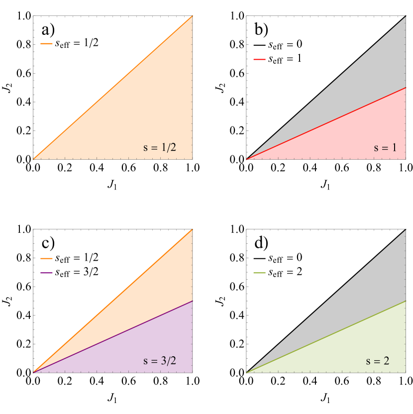
Figure 2: $(a)-(d)$ The $J_{2}$ vs. $J_{1}$ trimers’ ground state (colors) phase diagrams of $s=1/2$, $s=1$, $s=3/2$, and $s=2$ spin trimers, respectively . In all panels the upper straight lines denote $\alpha=J_{1}/J_{2}=1$, while the bottom ones denote $\alpha=1/2$. Since in real systems $\alpha<1$, white regions are unimportant.

References

- Stöhr and Siegmann [2006] J. Stöhr and H. C. Siegmann, Magnetism: From Fundamentals to Nanoscale Dynamics, Springer Series in Solid-State Sciences (Springer-Verlag, Berlin Heidelberg, 2006).
- White [2007] R. M. White, Quantum Theory of Magnetism Magnetic Properties of Materials (Springer, Berlin, 2007).
- Goodenough [1963] J. B. Goodenough, Magnetism And The Chemical Bond (John Wiley And Sons, 1963).
- Nguyen and Cava [2021] L. T. Nguyen and R. J. Cava, Chemical Reviews 121, 2935 (2021).
- Yin et al. [2017] C. Yin, G. Tian, G. Li, F. Liao, and J. Lin, RSC Advances 7, 33869 (2017).
- Nguyen et al. [2019] L. T. Nguyen, T. Kong, and R. J. Cava, Materials Research Express 6, 056108 (2019).
- Moessner and Ramirez [2006] R. Moessner and A. P. Ramirez, Physics Today 59, 24 (2006).
- Balents [2010] L. Balents, Nature 464, 199 (2010).
- Zhou et al. [2017] Y. Zhou, K. Kanoda, and T.-K. Ng, Reviews of Modern Physics 89, 025003 (2017).
- Nikuni et al. [2000] T. Nikuni, M. Oshikawa, A. Oosawa, and H. Tanaka, Physical Review Letters 84, 5868 (2000).
- Aczel et al. [2009] A. A. Aczel, Y. Kohama, C. Marcenat, F. Weickert, M. Jaime, O. E. Ayala-Valenzuela, R. D. McDonald, S. D. Selesnic, H. A. Dabkowska, and G. M. Luke, Physical Review Letters 103, 207203 (2009).
- Deisenhofer et al. [2006] J. Deisenhofer, R. M. Eremina, A. Pimenov, T. Gavrilova, H. Berger, M. Johnsson, P. Lemmens, H.-A. Krug von Nidda, A. Loidl, K.-S. Lee, and M.-H. Whangbo, Physical Review B 74, 174421 (2006).
- Singh and Johnston [2007] Y. Singh and D. C. Johnston, Physical Review B 76, 012407 (2007).
- Uchida et al. [2001] M. Uchida, H. Tanaka, M. I. Bartashevich, and T. Goto, Journal of the Physical Society of Japan 70, 1790 (2001).
- Uchida et al. [2002] M. Uchida, H. Tanaka, H. Mitamura, F. Ishikawa, and T. Goto, Physical Review B 66, 054429 (2002).
- Tsujii et al. [2005] H. Tsujii, B. Andraka, M. Uchida, H. Tanaka, and Y. Takano, Physical Review B 72, 214434 (2005).
- Lai and Valldor [2017] K. T. Lai and M. Valldor, Scientific Reports 7, 43767 (2017).
- Garcia et al. [2015] F. A. Garcia, U. F. Kaneko, E. Granado, J. Sichelschmidt, M. Holzel, J. G. S. Duque, C. A. J. Nunes, P. Marques-Ferreira, and R. Lora-Serrano, Physical Review B 91, 224416 (2015).
- Cantarino et al. [2019] M. R. Cantarino, R. P. Amaral, R. S. Freitas, J. C. R. Araujo, R. Lora-Serrano, H. Luetkens, C. Baines, S. Brauninger, V. Grinenko, R. Sarkar, H. H. Klauss, E. C. Andrade, and F. A. Garcia, Physical Review B 99, 054412 (2019).
- Komleva et al. [2020] E. V. Komleva, D. I. Khomskii, and S. V. Streltsov, Physical Review B 102, 174448 (2020).