Connected and Automated Vehicle Platoon Formation Control via Differential Games

Abstract

In this study, the connected and automated vehicles (CAVs) platooning problem is resolved under a differential game framework. Three information topologies are considered here. Firstly, the Predecessor-following (PF) topology is utilized where the vehicles control the distance with respect to the merely nearest predecessor via a sensor link-based information flow. Secondly, the Two-predecessor-following topology (TPF) is exploited where each vehicle controls the distance with respect to the two nearest predecessors. In this topology, the second predecessor is communicated via a Vehicle-to-vehicle (V2V) link. The individual trajectories of CAVs under the Nash equilibrium are derived in closed-form for these two information topologies. Finally, general information topology is examined and the differential game is formulated in this context. In all these options, Pontryagin’s principle is employed to investigate the existence and uniqueness of the Nash equilibrium and obtain its corresponding trajectories. In the general topology, we suppose numerical computation of eigenvalues and eigenvectors. Finally, the stability behavior of the platoon for the PF, TPF and general topologies are investigated. All these approaches represent promising and powerful analytical representations of the CAV platoons under the differential games. Simulation experiments have verified the efficiency of the proposed models and their solutions as well as their better results in comparison with the Model Predictive Control (MPC).

Keywords: Connected and automated vehicle (CAV); differential game; Model Predictive Control (MPC); Nash equilibrium; platoon control; Pontryagin’s principle; stability analysis

1 Introduction

Connected and automated vehicles (CAVs) and self-driving cars are promising technologies to enhance our daily experience of traveling with vehicles on the roads. The most common group behavior of CAVs is forming and maintaining platoons with short headways on the road [1]. To this end, CAVs need to exchange information via onboard sensors, Vehicle-to-Vehicle (V2V), Vehicle-to-Infrastructure (V2I), or Vehicle-to-Everything (V2X) communications. A platoon is defined as a closely-spaced group of vehicles driving with zero relative speed by maintaining a linear formation [2]. Such coordination is achieved by exchanging local information among the vehicles [3]. Platoons using wireless communications suffer time-varying delays and packet dropouts [4]. There are three types of platooning methods as designated in [5]. Leader-Follower approach in [6], Behavior-Based Approach in [7], and Virtual Structure approach in [8]. The behavior-based approach is associated with Artificial Potential Field (APF) in [9], flocking in [10], and swarm intelligence in [11]. Platoons can be classified in terms of the type of vehicles as truck platoons [12], underwater vehicles [13], unmanned aerial vehicles [14], and marine platoons [15].

Vehicle platoons offer remarkable benefits as listed in [16]. First of all, road capacity can be boosted due to the decrease in gaps between vehicles. Secondly, fuel consumption and emissions of pollutants can be decreased owing to the elimination of dispensable change of speed and aerodynamic drag on the pursuing vehicles. Besides, driving safety is potentially enhanced since the detection and actuation time are lessened compared to manual vehicles. Moreover, downstream traffic information can rapidly be transmitted upstream. Finally, passenger satisfaction can be enhanced since the system behavior is more reactive to changes in the traffic, and the shorter pursuing spaces can prevent cut-ins of other vehicles in the platoon. To sum up, vehicle platooning is a solution for traffic congestion and air pollution issues as stated in [2].

Differential games [17] and optimal control theory [18] have been widely applied to the vehicle platooning problem. Optimal control theory studied in [19] considers a single cost function optimized by the agents. On the other hand, differential games in [20] extend this idea to multiple cost functions each minimized by its relevant agent. Games can be cooperative or noncooperative. Differential games are ideally suited to model noncooperative dynamics where there is no central decision-maker. The corresponding solution concept for noncooperative games is the Nash equilibrium. While on the roads, the CAVs as rational agents comply with their interests and tend to strategies based on the Nash equilibrium resulting from a noncooperative game. In contrast, in an emergency such as after a collision, interacting vehicles have to be explicitly cooperative to stabilize themselves on the road and protect their safety as well as others [21]. Platooning under Nash optimality [22], intersection management with generalized Nash equilibrium [23], and lane-change via noncooperative game theory [24] are some of the CAVs problems solved by applying noncooperative games. In this paper, we propose a differential game-based platoon control scheme under the framework of noncooperative differential games. The analytical expressions and closed-form solutions corresponding to the Nash equilibrium are derived from Pontryagin’s minimum principle. Once the game is established, the Nash equilibrium-based trajectories are calculated beforehand and the CAVs follow their trajectories for the rest of time.

Research on differential game-based control of networked multi-agent systems has developed in three directions. These are Lyapunov stability analysis in [25] and numerical solution of Riccati Equations in [26] and numerical solution of Hamilton-Jacobi-Bellman (HJB) equations in [27]. However, explicit solution of players’ trajectories in differential game systems is studied only in a few research works and is left understudied in differential games-based networked control systems for vehicle platoons. Such explicit solutions enable fast simulations, reliable analysis, useful structural properties as well as a simple stability test. The main bottleneck of optimal control and differential games is the computational complexity of the underlying algorithms. Nevertheless, high complexity is not an issue for explicit expressions obtained in this study. The Model Predictive Control (MPC) and receding horizon control algorithms are other fast computational schemes in which they usually rely on linear approximations of the nonlinear system and its future behavior predictions over a small operating range [6, 28]. However, the proposed analytical approach is theoretically stronger than MPC since it does not rely on approximations and predictions.

In this study, our main contribution is to show that cooperative dynamics emerge from noncooperative decisions of vehicles. The problem that we examine is the one-dimensional point-to-point transportation of a vehicle team with coupled dynamics. The formulation of noncooperative games is based on Section 6.5.1 of [29]. We extend the PF topology investigated in [30] to the TPF and general topologies. This problem is crucial since it provides analytical insight into the platoon dynamics problem. We arrive at explicit Nash equilibrium derived in closed-form for the PF and TPF information topologies. We also obtain the solution of the differential game for general information topology that can be calculated numerically.

Stability is an essential requirement for a platoon. There are two types of stabilities: individual or internal stability and string stability. String stability can be defined mathematically as certain sufficient conditions of the inter-vehicles distancing policy errors, velocity or acceleration transfer functions [31]. The platoon is necessarily string stable if these sufficient conditions hold. In an internally stable platoon system, inter-vehicles distancing policy error of each following vehicle reduces to zero at a steady state or simply, the vehicle converges to the given trajectory [32]. String stability conditions ensure that the exogenous disturbances and spacing policy errors do not propagate from the predecessor vehicles along the vehicle string [33]. We investigate both internal stability and string stability under the proposed differential game framework for CAVs platooning. We show that the internal stability of the platoon system is achieved. While it is not straightforward to prove string stability explicitly, we have established its sufficient condition for the PF topology and have left the other topologies for future work. Finally, the CAVs platooning problem is resolved using the MPC method. To that end, the proposed differential games are converted to the standard matrix expressions through the use of graph theory and graph Laplacian matrix. Simulation results justified all models and solutions.

The rest of the manuscript is organized as follows. In Section 2, the problem definition, the main results and proofs are highlighted. Section 3 discusses the MPC-based platoon control. In Section 4, simulation results are demonstrated. Finally, Section 5 is dedicated to the conclusions and future work.

2 Platoon formation control

This section presents the game theory approach to vehicle platoon formation control. We consider a simplified kinematic model of vehicles in which the control input directly affects the velocity. The platoon is characterized based on the communication topology (CT) and inter-vehicle distances between each CAV and the preceding. Differential game-based formulations of the platoon formation control under the PF and TPF topologies are presented in the subsections 2.1 and 2.2, respectively. We have derived the associated individual state trajectories with the Nash equilibrium actions for the vehicles. The analytical expressions reveal explicitly the role of the influencing factors on the evolution of platooning dynamic behavior. Afterward, we extend the differential game formulation to involve general topology. We show that the proposed differential game problem under the general topology is convex and the control inputs can be computed efficiently.

2.1 Predecessor-following (PF) Topology

Information exchange among the vehicles via a connected information topology is necessary for platoon formation control. Following [34], we distinguish between connection links among vehicles by categorizing them into V2V connection links and sensor connection links. A sensor link emphasizes the information flow from the predecessor vehicle to the ego vehicle (see Figure 1). A V2V connection link between a pair of vehicles can be one of rearward, forward, and bidirectional connection link types.

Consider a platoon of $n$ CAVs under the PF topology as shown in Figure 1. CAVs move along the center of a single lane, all in the same traffic flow. Under this topology, each vehicle must follow its predecessor by adjusting its inter-vehicle distance $d_{i}$ using the relative displacement information acquired through the unidirectional sensor link. Note that $d_{i}$ can be regarded as the length of vehicle $i$ appended to the measured inter-vehicle distance with its predecessor vehicle. We assume that the actual leading vehicle of the platoon indexed by 1 follows a reference trajectory indexed by 0. The reference ($x_{0}$) is either a manned/unmanned vehicle on the road or simply a reference trajectory generated by a driver-assistive technology such as Lane Following Assist (LFA). The actual vehicles of the platoon are indexed as $1,\ldots,n$. We employ a single-integrator model to govern the longitudinal dynamics of the vehicles [35]. Under a hierarchical control scheme [36, 37], this model at the top of the hierarchy provides the control input that directly affects the longitudinal velocities of the vehicles to maintain desired inter-vehicle distances. At the bottom of the hierarchy, a low-level controller adjusts the actuation of each vehicle at the throttle and brake level to achieve the desired velocities.

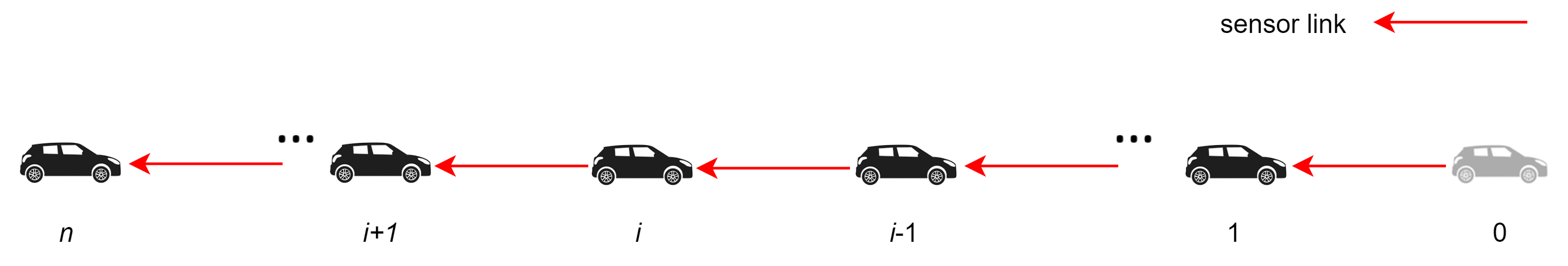
Figure 1: A vehicle platoon with predecessor-following (PF) topology.

Let $x_{i}$ and $u_{i}$ denote the $i$th vehicle’s longitudinal position and velocity/control input ($i=1,\ldots,n$), respectively. The relative longitudinal displacement dynamics can be described as

$$\dot{x}_{i}-\dot{x}_{i-1}=u_{i}.$$ (1)

The platoon formation control cost function for vehicle $i$ ($i=1,\ldots,n$) is defined as

$$J_{i}(x_{i},x_{i-1},u_{i})=\frac{1}{2}\int_{0}^{t_{f}}(\omega_{i}(x_{i}-x_{i-1}-d_{i})^{2}+u_{i}^{2})~{}\mathrm{dt},$$ (2)

where $t_{f}$ is the terminal time and $\omega_{i}>0$ is a sensor link-related weighting parameter. The weighting parameter $\omega_{i}$ penalizes the inter-vehicle displacement and each vehicle can adjust this parameter taking its own interests or other personal factors such as fuel amount in the tank into account. We note that the PF topology is a collision-free platoon formation. Using the sensory information, each vehicle is aware of its relative displacement to its predecessor and regulates its velocity to acquire and preserve the inter-vehicle distancing policy then. Since there are no V2V communications among the vehicles, this information exchange network is not subject to external hacks or misinformation sent by a vehicle. Therefore, a connected environment is not necessary for this model.

Assumption 1.

(Collision-avoidance) The initial positions hold $x_{0}(0)>x_{1}(0)>\cdots>x_{n}(0)$.

Under Assumption 1, collision-avoidance is embedded in the platoon formation control given by (1) and (2). Furthermore, the inter-vehicle distancing policies are defined as negative values, i.e., $d_{i}<0$ ($i=1,\ldots,n$). This is because the longitudinal relative displacement of vehicles have a direction opposite to the traffic flow. In other words, under Assumption 1 the relative displacements $x_{i}-x_{i-1}$ are resulting in negative values.

Assumption 2.

(Reference trajectory) We assume $\dot{x}_{0}=c$ where $c$ is a constant, i.e., the reference has a constant speed.

The dynamics and cost function in (1) and (2) demand the position information of the following vehicle and its predecessor. In the following, we transform these equations into a new dynamics and cost function that does not require the individual positions but the relative displacement acquired via the sensor links.

Let’s define the relative displacement $y_{i}=x_{i}-x_{i-1}$ for vehicle $i$ ($i=1,\ldots,n$) that can be directly measured via the sensor link. The platoon formation control in (1) and (2) as a non-cooperative differential game can be redefined as the minimization of the following optimization

$$\quad\min_{u_{i}}~{}J_{i}(y_{i},u_{i})=\frac{1}{2}\int_{0}^{t_{f}}(\omega_{i}(y_{i}-d_{i})^{2}+u_{i}^{2})~{}dt,$$ (3)

$${s.t.}$$

$$\quad\dot{y}_{i}=u_{i},\quad y_{i}(0)=x_{i}(0)-x_{i-1}(0),\quad i=1,\ldots,n.$$

We present the closed-form solutions to the associated relative displacement trajectories with the Nash equilibrium as follows.

Theorem 1.

For an $n$-vehicle platoon defined as the noncooperative differential game (3):

1. There is a unique Nash equilibrium of relative displacement control actions $u_{i}$’s.

2. The associated relative displacement trajectories with the Nash equilibrium $y_{i}$’s are given by

   $$y_{i}(t)=\alpha_{i}(t)y_{i}(0)+(\alpha_{i}(t)-1)d_{i},$$ (4)

   where

   $$\alpha_{i}(t)=\frac{\mathrm{cosh}(\sqrt{\omega_{i}}(t_{f}-t))}{\mathrm{cosh}(\sqrt{\omega_{i}}t_{f})}.$$ (5)

Proof.

Define the Hamiltonian

$$H_{i}(y_{i},u_{i},\lambda_{i})=\frac{1}{2}(\omega_{i}(y_{i}-d_{i})^{2}+u_{i}^{2})+\lambda_{i}u_{i},\quad i=1,\ldots,n,$$ (6)

where $\lambda_{i}$ is the costate. According to the Pontryagin’s minimum principle, the necessary conditions for optimality are $\frac{\partial H_{i}}{\partial u_{i}}=0$ and $\dot{\lambda}_{i}=-\frac{\partial H_{i}}{\partial y_{i}}$. Applying the necessary conditions on (6) yields:

$$u_{i}=-\lambda_{i}$$ (7)

$$\dot{\lambda}_{i}=-\omega_{i}y_{i}+\omega_{i}d_{i},\quad\lambda_{i}(t_{f})=0,$$ (8)

for $i=1,\ldots,n$.

Substituting (7) in relative dynamics results in

$$\dot{y}_{i}=-\lambda_{i},\quad y_{i}(0)=x_{i}(0)-x_{i-1}(0),\quad i=1,\ldots,n.$$ (9)

Let $\bm{y}=[y_{1},\ldots,y_{n}]^{\top}\in\mathit{\mathbb{R}}^{n}$, $\bm{\lambda}=[\lambda_{1},\ldots,\lambda_{n}]^{\top}\in\mathit{\mathbb{R}}^{n}$, $\bm{d}=[d_{1},\ldots,d_{n}]^{\top}\in\mathit{\mathbb{R}}^{n}$, $\bm{A}=\mathrm{diag}(\omega_{1},\ldots,\omega_{n})\in\mathit{\mathbb{R}}^{n}$, and $\bm{\omega}=\bm{A}\bm{d}$. Also, let ${\bf 0}$ and $\bm{I}$ denote the zero and identity matrix of appropriate dimension. The equations (7), (8) and (9) can be unified into the following differential equation

$$\begin{bmatrix}\dot{\bm{y}}\\ \dot{\bm{\lambda}}\end{bmatrix}=\begin{bmatrix}{\bf 0}&-\bm{I}\\ -\bm{A}&{\bf 0}\end{bmatrix}\begin{bmatrix}\bm{y}\\ \bm{\lambda}\end{bmatrix}+\begin{bmatrix}{\bf 0}\\ \bm{\omega}\end{bmatrix},$$ (10)

with the initial condition vector $\bm{y}(0)$ where $y_{i}(0)=x_{i}(0)-x_{i-1}(0)$ ($i=1,\ldots,n$) and terminal condition vector $\bm{\lambda}(t_{f})$ where $\lambda_{i}(t_{f})=0$ ($i=1,\ldots,n$).

If there is a unique Nash equilibrium solution, then equation (10) has a solution for every $\bm{y}(0)$ and $\bm{\lambda}(t_{f})$. Matrix analyses in the Laplace Transform domain then show that (10) has a solution as follows

$$\begin{bmatrix}\bm{y}\\ \bm{\lambda}\end{bmatrix}={\bf\Phi}(t)\begin{bmatrix}\bm{y}(0)\\ \bm{\lambda}(0)\end{bmatrix}+{\bf\Psi}(t,0)\bm{\omega},$$ (11)

where

$$\bm{\Phi}(t)= \begin{bmatrix}\bm{\Phi}_{11}(t)&\bm{\Phi}_{12}(t)\\ \bm{\Phi}_{21}(t)&\bm{\Phi}_{22}(t)\end{bmatrix}=\mathcal{L}^{-1}\{\begin{bmatrix}s\bm{I}&\bm{I}\\ \bm{A}&s\bm{I}\end{bmatrix}^{-1}\}=$$ (12)

$$\mathcal{L}^{-1}\{\begin{bmatrix}s(s^{2}\bm{I}-\bm{A})^{-1}&-(s^{2}\bm{I}-\bm{A})^{-1}\\ -\bm{A}(s^{2}\bm{I}-\bm{A})^{-1}&s(s^{2}\bm{I}-\bm{A})^{-1}\end{bmatrix}\}=\begin{bmatrix}\mathrm{cosh}(\bm{A}^{\frac{1}{2}}t)&-\mathrm{sinh}(\bm{A}^{\frac{1}{2}}t)\bm{A}^{-\frac{1}{2}}\\ -\bm{A}^{\frac{1}{2}}\mathrm{sinh}(\bm{A}^{\frac{1}{2}}t)&\mathrm{cosh}(\bm{A}^{\frac{1}{2}}t)\end{bmatrix},$$

and

$$\bm{\Psi}(t,0)=\begin{bmatrix}\bm{\Psi}_{1}(t,0)\\ \bm{\Psi}_{2}(t,0)\end{bmatrix}=\int_{0}^{t}\begin{bmatrix}\bm{\Phi}_{12}(t-\tau)\\ \bm{\Phi}_{22}(t-\tau)\end{bmatrix}d\tau=\begin{bmatrix}-(\bm{I}-\mathrm{cosh}(\bm{A}^{\frac{1}{2}}t))\bm{A}^{-1}\\ -\mathrm{sinh}(\bm{A}^{\frac{1}{2}}t)\bm{A}^{-\frac{1}{2}}\end{bmatrix}.$$ (13)

From (11), $\bm{y}$ and $\bm{\lambda}$ are obtained as

$$\bm{y}=\bm{\Phi}_{11}(t)\bm{y}(0)+\bm{\Phi}_{12}(t)\bm{\lambda}(0)+\bm{\Psi}_{1}(t,0)\bm{\omega},$$ (14)

$$\bm{\lambda}=\bm{\Phi}_{21}(t)\bm{y}(0)+\bm{\Phi}_{22}(t)\bm{\lambda}(0)+\bm{\Psi}_{2}(t,0)\bm{\omega}.$$ (15)

Applying the terminal condition $\bm{\lambda}(t_{f})={\bf 0}$, we obtain vector $\bm{\lambda}(0)$ as

$$\bm{\lambda}(0)=\bm{\Phi}_{22}^{-1}(t_{f})\left[-\bm{\Phi}_{21}(t_{f})\bm{y}(0)-\bm{\Psi}_{2}(t_{f},0)\bm{\omega}\right].$$ (16)

Notice that the existence of $\bm{\Phi}_{22}^{-1}(t_{f})$ (which also means the existence of a unique Nash equilibrium solution) and $\bm{\Psi}_{2}(t_{f},0)$ for all $t_{f}>0$ can be realized from the definition of the hyperbolic functions. Since $\bm{A}$ is diagonal, therefore, $\mathrm{sinh}(\bm{A}^{\frac{1}{2}}t_{f})$ and $\mathrm{cosh}(\bm{A}^{\frac{1}{2}}t_{f})$ are diagonal matrices with the diagonal elements of $\mathrm{sinh}(\sqrt{\omega_{i}}t)>0$ and $\mathrm{cosh}(\sqrt{\omega_{i}}t)>0$ for $i=1,\ldots,n$, respectively as $\omega_{i}>0$.

Finally, substituting (16) into (14) and after simplifications, the associated relative displacement trajectories with the Nash equilibrium $y_{i}$’s are obtained as in (4). ∎

The unique Nash equilibrium control actions $u_{i}$’s and the individual vehicle trajectories $x_{i}$’s can be calculated from (4).

2.2 Two-predecessor-following (TPF) Topology

Sometimes during the platoon formation control the sensor link can be unavailable due to, for example, hardware problems in the sensors. In such a situation, collision with the preceding or following vehicle is an immediate danger since the formation control cannot be maintained. Therefore, a more reliable than the PF but still relatively simple vehicle platoon topology can be the Two-predecessor-following (TPF) topology as shown in Figure 2. Under this topology, if the sensor link from the preceding vehicle is not available to the vehicle $i$, a rearward V2V link from the second preceding vehicle is still available to maintain the platoon formation control.

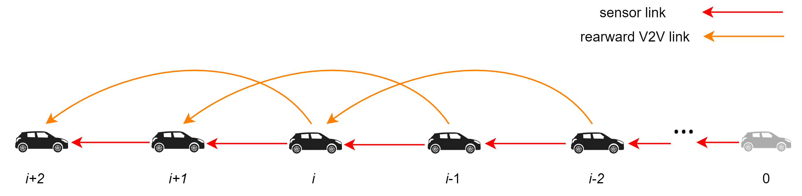
Figure 2: Two-predecessor-following (TPF) topology in the connected environment.

The platoon formation control cost function for vehicle $i$ ($i=1,\ldots,n$) under the TPF topology is defined as

$$J_{i}(x_{i},x_{i-1},x_{i-2},u_{i})=\frac{1}{2}\int_{0}^{t_{f}}\Big{(}\omega_{i}(x_{i}-x_{i-1}-d_{i})^{2}+\tilde{\omega}_{i}\big{(}x_{i}-x_{i-2}-(d_{i}+d_{i-1})\big{)}^{2}+u_{i}^{2}\Big{)}~{}\mathrm{dt},$$ (17)

where $\tilde{\omega}_{i}>0$ is the V2V communication link-related weighting parameter.

Using the relative displacement $y_{i}$’s, the platoon formation control under the TPF topology as a non-cooperative differential game can be redefined as the minimization of the following optimization

$$\quad\min_{u_{i}}~{}J_{i}(y_{i},y_{i-1},u_{i})=\frac{1}{2}\int_{0}^{t_{f}}\Big{(}\omega_{i}(y_{i}-d_{i})^{2}+\tilde{\omega}_{i}\big{(}(y_{i}-d_{i})+(y_{i-1}-d_{i-1})\big{)}^{2}+u_{i}^{2}\Big{)}~{}\mathrm{dt},$$ (18)

$${s.t.}$$

$$\quad\dot{y}_{i}=u_{i},\quad,y_{i}(0)=x_{i}(0)-x_{i-1}(0),\quad i=1,\ldots,n.$$

Before we present the closed-form solutions to the associated individual (relative displacement) trajectories with the Nash equilibrium, the following facts and lemma are given first.

Fact 1.

The determinant of an upper (or lower) triangular or diagonal matrix is the product of the (main) diagonal entries [38].

Fact 2.

Let $\bm{B}\in\mathit{\mathbb{R}}^{n}$ be a nonsingular matrix. Then, $\bm{B}^{-1}$ is upper (lower) triangular if and only if $\bm{B}$ is upper (lower) triangular (Fact 3.20.5. in [39]).

Lemma 1.

The matrix

$$\bm{A}= \begin{bmatrix}\omega_{1}&0&0&0&\cdots&0\\ 0&\omega_{2}&0&0&\cdots&0\\ 0&\tilde{\omega}_{3}&\tilde{\omega}_{3}+\omega_{3}&0&\cdots&0\\ \vdots&\ddots&&\ddots&&\vdots\\ 0&0&\cdots&0&\tilde{\omega}_{n}&\tilde{\omega}_{n}+\omega_{n}\end{bmatrix},$$ (19)

can be factorized as

$$\bm{A}=\bm{V}\bm{D}\bm{V}^{-1},$$ (20)

where

$$\bm{D}=\mathrm{diag}[\cdots,\delta_{i},\cdots],$$ (21)

$$\bm{V}=[\cdots,\bm{v}_{i},\cdots],$$ (22)

$$\bm{V}^{-1}=[\cdots,\bm{\tilde{v}}_{i},\cdots],$$ (23)

$$\delta_{i}=\left\{\begin{array}[]{ll}\omega_{i}&\quad\mbox{, $i=1,2$ }\\ &\\ \tilde{\omega}_{i}+\omega_{i}&\quad\mbox{, $i=3,\cdots,n$ },\\ \end{array}\right.$$ (27)

$$\bm{v}_{1}=[\eta_{1}^{1},0,\cdots,0]^{\top},$$ (28)

$$\bm{v}_{i}=[0,\cdots,0,\eta_{i}^{j},-\frac{\tilde{\omega}_{j}\eta_{i}^{j-1}}{\tilde{\omega}_{j}+\omega_{j}-\delta_{i}},\cdots,-\frac{\tilde{\omega}_{n}\eta_{i}^{n-1}}{\tilde{\omega}_{n}+\omega_{n}-\delta_{i}}]^{\top},\quad j=i,\cdots,n,\quad i=2,\cdots,n-1,$$ (29)

$$\bm{v}_{n}=[0,\cdots,0,\eta_{n}^{n}]^{\top},$$ (30)

$$\bm{\tilde{v}}_{1}=[\zeta_{1}^{1},0,\cdots,0]^{\top},$$ (31)

$$\bm{\tilde{v}}_{i}=[0,\cdots,0,\zeta_{i}^{j},\frac{\tilde{\omega}_{j}-\eta_{i}^{j}\zeta_{i}^{i}\delta_{i}}{\eta_{j}^{j}\delta_{j}},-\frac{\sum_{k=i}^{j-1}\eta_{k}^{j}\zeta_{i}^{k}\delta_{k}}{\eta_{j}^{j}\delta_{j}},\cdots]^{\top},\quad j=i,\quad i=2,\cdots,n-1,$$ (32)

$$\bm{\tilde{v}}_{n}=[0,\cdots,0,\zeta_{n}^{n}]^{\top},$$ (33)

$$\zeta_{i}^{i}=\frac{1}{\eta_{i}^{i}},\quad i=1,\cdots,n.$$ (34)

Proof.

The eigenvalues of $\bm{A}$ are the roots of its characteristic polynomial $\rho(\delta)$:

$$\rho(\delta)= \det(\bm{A}-\delta\bm{I}),$$ (35)

where $\delta$ is an unknown variable representing the unknown eigenvalues. According to Fact 1, (35) simplifies as

$$\rho(\delta)= \prod_{i=1}^{2}(\omega_{i}-\delta)\prod_{i=3}^{n}\Big{(}(\tilde{\omega}_{i}+\omega_{i})-\delta)\Big{)}.$$ (36)

Solving (36) for its roots, the eigenvalues of $\bm{A}$ are obtained as (27). As all of its eigenvalues are real and positive ($\delta_{i}>0$ for $i=1,\ldots,n$), the matrix $\bm{A}$ is positive definite.

From (36), it can be easily seen that the algebraic and geometric multiplicities of eigenvalue $\delta_{i}$ are both equal to 1 for all $i=1,\ldots,n$. Therefore, $\bm{A}\in\mathit{\mathbb{R}}^{n}$ has $n$ linearly independent eigenvectors and can be factorized as in (20) where the modal matrix $\bm{V}=[\bm{v}_{1},\cdots,\bm{v}_{n}]\in\mathit{\mathbb{R}}^{n}$ and diagonal matrix $\bm{D}=\mathrm{diag}(\delta_{1},\cdots,\delta_{n})\in\mathit{\mathbb{R}}^{n}$ are constituted from the eigenvectors and eigenvalues of $\bm{A}$, respectively.

Now, we show that the vectors $\bm{v}_{i}$ given by (29) and (30) are the right eigenvectors associated with $\delta_{i}$ ($i=2,\ldots,n$). The right eigenvector satisfies

$$(\bm{A}-\delta_{i}\bm{I})\bm{v}_{i}=\bm{0}.$$ (37)

The $j$th row of $\bm{A}-\delta_{i}\bm{I}$ has two non-zero elements, namely $\tilde{\omega}_{j}$ and $(\tilde{\omega}_{j}+\omega_{j})-\delta_{i}$ at the indices $i-1$ and $i$, respectively. Then, the right side of (37) reduces to $\left[(\tilde{\omega}_{j}+\omega_{j})-\delta_{i}\right]\eta_{i}^{i}$. Inside the bracket always equals to zero. Similarly, it can be verified that $\bm{v}_{1}$ given by (28) satisfies (37). Therefore, $\bm{v}_{i}$ satisfies (37) for all $i=1,\ldots,n$. From (20) and using Fact 2 the matrix $\bm{V}^{-1}$ can be determined in form of (23) and (31)-(34). ∎

Note that based on Lemma 1, we have

$$\bm{A}^{\frac{1}{2}}=\bm{V}\bm{D}^{\frac{1}{2}}\bm{V}^{-1},\quad\mathrm{sinh}(\bm{A}^{\frac{1}{2}})=\bm{V}\mathrm{sinh}(\bm{D}^{\frac{1}{2}})\bm{V}^{-1},$$

$$\mathrm{cosh}(\bm{A}^{\frac{1}{2}})=\bm{V}\mathrm{cosh}(\bm{D}^{\frac{1}{2}})\bm{V}^{-1},\quad(\mathrm{cosh}(\bm{A}^{\frac{1}{2}}))^{-1}=\bm{V}^{-1}\mathrm{cosh}(\bm{D}^{-\frac{1}{2}})\bm{V}.$$ (38)

The associated relative trajectories $y_{i}$’s with the Nash equilibrium are presented below.

Theorem 2.

For an $n$-vehicle platoon under the TPF topology defined as the noncooperative differential game (18):

1. There is a unique Nash equilibrium.

2. The associated relative displacement trajectories with the Nash equilibrium are given by

   $$y_{i}(t)=\left\{\begin{array}[]{ll}\alpha_{i}^{i}(t)y_{i}(0)+(\alpha_{i}^{i}(t)-1)d_{i}&\quad\mbox{$i=1,2$ }\\ &\\ \sum_{k=2}^{i}\alpha_{k}^{i}(t)y_{k}(0)+\sum_{k=2}^{i-1}\alpha_{k}^{i}(t)d_{k}+(\alpha_{i}^{i}(t)-1)d_{i}&\quad\mbox{$i=3,\cdots,n$ },\\ \end{array}\right.$$ (42)

   where

   $$\alpha_{i}^{i}(t)=\left\{\begin{array}[]{ll}\frac{\mathrm{cosh}(\sqrt{\omega_{i}}(t_{f}-t))}{\mathrm{cosh}(\sqrt{\omega_{i}}t_{f})}&\quad\mbox{$i=1,2$ }\\ &\\ \frac{\mathrm{cosh}(\sqrt{\tilde{\omega}_{i}+\omega_{i}}(t_{f}-t))}{\mathrm{cosh}(\sqrt{\tilde{\omega}_{i}+\omega_{i}}t_{f})}&\quad\mbox{$i=3,\cdots,n$ }\\ \end{array}\right.$$ (46)

   $$\alpha_{i}^{j}(t)=\sum_{k=i}^{j}\eta_{k}^{j}\zeta_{i}^{k}\alpha_{k}^{k}(t)\quad\quad,i\neq j,i=2,\cdots,n,j=3,\cdots,n.$$ (47)

Proof.

Applying the necessary conditions for optimality on the Hamiltonians yields

$$u_{i}=-\lambda_{i}$$ (48)

$$\dot{\lambda}_{i}=-\omega_{i}(y_{i}-d_{i})-\tilde{\omega}_{i}(y_{i}-d_{i}+y_{i-1}-d_{i-1}),\quad\lambda_{i}(t_{f})=0$$ (49)

and

$$\dot{y}_{i}=-\lambda_{i},\quad y_{i}(0)=x_{i}(0)-x_{i-1}(0)$$ (50)

for $i=1,\ldots,n$.

Applying the terminal condition $\bm{\lambda}(t_{f})={\bf 0}$ and using (2.2), vector $\bm{\lambda}(0)$ after simplification is obtained as

$$\bm{\lambda}(0)= (\mathrm{cosh}(\bm{A}^{\frac{1}{2}}t_{f}))^{-1}\left[\bm{A}^{\frac{1}{2}}\mathrm{sinh}(\bm{A}^{\frac{1}{2}}t_{f})\bm{y}(0)+\mathrm{sinh}(\bm{A}^{\frac{1}{2}}t_{f})\bm{A}^{-\frac{1}{2}}\bm{\omega}\right]$$

$$= \bm{V}(\mathrm{cosh}(\bm{D}^{\frac{1}{2}}t_{f}))^{-1}\bm{V}^{-1}\left[\bm{V}\bm{D}^{\frac{1}{2}}\mathrm{sinh}(\bm{D}^{\frac{1}{2}}t_{f})\bm{V}^{-1}\bm{y}(0)+\bm{V}\bm{D}^{\frac{1}{2}}\mathrm{sinh}(\bm{D}^{\frac{1}{2}}t_{f})\bm{V}^{-1}\bm{d}\right]$$

$$= \bm{V}(\mathrm{cosh}(\bm{D}^{\frac{1}{2}}t_{f}))^{-1}\bm{D}^{\frac{1}{2}}\mathrm{sinh}(\bm{D}^{\frac{1}{2}}t_{f})\bm{V}^{-1}\left[\bm{y}(0)+\bm{d}\right].$$ (51)

Substituting $\bm{\lambda}(0)$ from (2.2), $\bm{y}$ is simplified as

$$\bm{y}= \mathrm{cosh}(\bm{A}^{\frac{1}{2}}t)\bm{y}(0)-\mathrm{sinh}(\bm{A}^{\frac{1}{2}}t)\bm{A}^{-\frac{1}{2}}\bm{\lambda}(0)-(\bm{I}-\mathrm{cosh}(\bm{A}^{\frac{1}{2}}t))\bm{d}$$

$$= \bm{V}\mathrm{cosh}(\bm{D}^{\frac{1}{2}}t)\bm{V}^{-1}\bm{y}(0)-\bm{V}\mathrm{sinh}(\bm{D}^{\frac{1}{2}}t)\bm{D}^{-\frac{1}{2}}\bm{V}^{-1}$$

$$\left[\bm{V}(\mathrm{cosh}(\bm{D}^{\frac{1}{2}}t_{f}))^{-1}\bm{D}^{\frac{1}{2}}\mathrm{sinh}(\bm{D}^{\frac{1}{2}}t_{f})\bm{V}^{-1}(\bm{y}(0)+\bm{d})\right]+\bm{V}\mathrm{cosh}(\bm{D}^{\frac{1}{2}}t)\bm{V}^{-1}\bm{d}-\bm{d}$$

$$= \left[\bm{V}\mathrm{cosh}(\bm{D}^{\frac{1}{2}}t)\bm{V}^{-1}-\bm{V}(\mathrm{cosh}(\bm{D}^{\frac{1}{2}}t_{f}))^{-1}\mathrm{sinh}(\bm{D}^{\frac{1}{2}}t)\mathrm{sinh}(\bm{D}^{\frac{1}{2}}t_{f})\bm{V}^{-1}\right]\bm{y}(0)+$$

$$\left[\bm{V}\mathrm{cosh}(\bm{D}^{\frac{1}{2}}t)\bm{V}^{-1}-\bm{V}(\mathrm{cosh}(\bm{D}^{\frac{1}{2}}t_{f}))^{-1}\mathrm{sinh}(\bm{D}^{\frac{1}{2}}t)\mathrm{sinh}(\bm{D}^{\frac{1}{2}}t_{f})\bm{V}^{-1}-\bm{I}\right]\bm{d}.$$ (52)

Let

$$\bm{P}= \bm{V}\mathrm{cosh}(\bm{D}^{\frac{1}{2}}t)\bm{V}^{-1}-\bm{V}(\mathrm{cosh}(\bm{D}^{\frac{1}{2}}t_{f}))^{-1}\mathrm{sinh}(\bm{D}^{\frac{1}{2}}t)\mathrm{sinh}(\bm{D}^{\frac{1}{2}}t_{f})\bm{V}^{-1}$$

$$= \bm{V}\left[\mathrm{cosh}(\bm{D}^{\frac{1}{2}}t)-(\mathrm{cosh}(\bm{D}^{\frac{1}{2}}t_{f}))^{-1}\mathrm{sinh}(\bm{D}^{\frac{1}{2}}t)\mathrm{sinh}(\bm{D}^{\frac{1}{2}}t_{f})\right]\bm{V}^{-1}$$

$$= \bm{V}\left[\mathrm{cosh}(\bm{D}^{\frac{1}{2}}(t_{f}-t))(\mathrm{cosh}(\bm{D}^{\frac{1}{2}}t_{f}))^{-1}\right]\bm{V}^{-1}$$

$$= \bm{V}\bm{\Delta}\bm{V}^{-1}.$$ (53)

Here, $\bm{\Delta}=\mathrm{diag}[\cdots,\alpha_{i}^{i},\cdots]$ where $\alpha_{i}^{i}$ are given by (46) and $\bm{P}$ has the following form

$$\bm{P}=\begin{bmatrix}\alpha_{1}^{1}&0&0&0&\cdots&0\\ 0&\alpha_{2}^{2}&0&0&\cdots&0\\ 0&\alpha_{2}^{3}&\alpha_{3}^{3}&0&\cdots&0\\ \vdots&\vdots&&\ddots&&\vdots\\ 0&\alpha_{2}^{n}&\alpha_{3}^{n}&\cdots&\alpha_{n-1}^{n}&\alpha_{n}^{n}\end{bmatrix},$$ (54)

where its non-diagonal nonzero elements $\alpha_{i}^{j}$ are given by (47).

Now, we get vector $\bm{y}$ in terms of $\bm{P}$ as

$$\bm{y}= \bm{P}\bm{y}(0)+(\bm{P}-\bm{I})\bm{d}.$$ (55)

From (55) the individual trajectories $y_{i}$’s are derived as in (42). ∎

2.3 General Topology

In this study, we assume that the vehicles are connected via the rearward V2V and sensor links, so the information flow is only backward in the opposite direction of the traffic flow. In the following, we extend the proposed differential game approach to platoon formation control from the PF and TPF topologies to general topology.

The platoon formation control cost function for vehicle $i$ ($i=1,\ldots,n$) under general topology is defined

$$J_{i}(x_{1},\cdots,x_{n},u_{i})=\frac{1}{2}\int_{0}^{t_{f}}\Big{(}\sum_{j\in\mathcal{N}_{i}}\omega_{ij}\big{(}x_{i}-x_{j}-\sum_{k=j+1}^{i}d_{k}\big{)}^{2}+u_{i}^{2}\Big{)}~{}\mathrm{dt},$$ (56)

where $\omega_{ij}\geq 0$ and $\mathcal{N}_{i}$ is the set of vehicles in the platoon directly connected to the vehicle $i$ either via a sensor link or (rearward) V2V connection link.

The platoon formation control under general topology as a noncooperative differential game can be redefined as the minimization of the following optimization

$$\min_{u_{i}}~{}J_{i}(y_{j\in\mathcal{N}_{i}},u_{i})=\frac{1}{2}\int_{0}^{t_{f}}\Big{(}\sum_{j\in\mathcal{N}_{i}}\omega_{ij}\left[\sum_{k=j+1}^{i}(y_{k}-d_{k})\right]^{2}+u_{i}^{2}\Big{)}~{}\mathrm{dt}$$ (57)

s.t.

$$\quad\dot{y}_{i}=u_{i},\quad,y_{i}(0)=x_{i}(0)-x_{i-1}(0),\quad i=1,\ldots,n.$$

The information structure of the proposed differential games under the PF and TPF topologies depicted in $\bm{A}$ is rather straightforward. However, due to its complex information structure, finding closed-form individual trajectories for platoon formation control under general topology as a noncooperative differential game (57) is highly analytically intricate. The following theorem presents results regarding the solution of this optimization.

Theorem 3.

For an $n$-vehicle platoon under general topology defined as the noncooperative differential game (57):

1. There is a unique Nash equilibrium of relative displacements control actions $u_{i}$’s.

2. The associated relative displacement trajectories with the Nash equilibrium are obtained as in (14).

Proof.

Applying the necessary conditions for optimality on the Hamiltonian yields

$$\dot{\lambda}_{i}=-\sum_{j\in\mathcal{N}_{i}}\omega_{ij}\sum_{k=j+1}^{i}(y_{k}-d_{k}),\quad\lambda_{i}(t_{f})=0,$$ (58)

for $i=1,\ldots,n$.

From (58), the platoon information matrix $\bm{A}\in\mathit{\mathbb{R}}^{n}$ under general topology is defined as

$$\bm{A}= \begin{bmatrix}\sum_{j\in N_{1}}w_{1j}&0&\cdots&0\\ \sum_{j\in N_{2},j<1}w_{2j}&\sum_{j\in N_{2}}w_{2j}&0&0\\ \vdots&\vdots&\ddots&\vdots\\ \sum_{j\in N_{n},j<1}w_{nj}&\sum_{j\in N_{n},j<2}w_{nj}&\cdots&\sum_{j\in N_{n}}w_{nj}\end{bmatrix}.$$ (59)

Following the solution procedure in proof of Theorem 1, the differential equation (10) can be formed where its solution is given by (11). From this equation, the associated platoon’s relative displacement trajectories with the Nash equilibrium are obtained as in (14). It can be seen that the calculation of the trajectories requires substituting the vector $\bm{\lambda}(0)$ from (16). This vector exists if and only if matrices $\bm{\Phi}_{22}^{-1}(t_{f})$ and $\bm{A}^{\pm\frac{1}{2}}$ exist.

The eigenvalues of $\bm{A}$ are obtained from its characteristic polynomial (35). This equation simplifies as

$$\rho(\delta)= \prod_{i=1}^{n}(\sum_{j\in N_{i}}w_{ij}-\delta).$$ (60)

From (60), the eigenvalues of $\bm{A}$ are $\delta_{i}=\sum_{j\in N_{i}}w_{ij}$ where all are real and positive ($\delta_{i}>0$ for $i=1,\ldots,n$) and $\bm{A}$ is positive definite. Additionally, we can see that both algebraic and geometric multiplicities of eigenvalue $\delta_{i}$ are 1 for all $i=1,\ldots,n$. Thus, there exist a diagonal matrix $\bm{D}$ and a modal matrix $\bm{V}$ in form of (21) and (22) and are constituted from the eigenvectors and eigenvalues of $\bm{A}$, respectively, and $\bm{A}$ is factorized as in (20). Consequently, matrices $\bm{\Phi}_{22}^{-1}(t_{f})$ and $\bm{A}^{\pm\frac{1}{2}}$ exist and can be calculated from (2.2). ∎

2.4 Stability Analysis

Individual stability refers to vehicles’ relative displacement trajectories $y_{i}(t)$s converging to the desired inter-vehicles distancing policies $d_{i}$s. String stability simply refers to distancing errors and disturbances not amplifying when propagating along the vehicle string [40]. In the following, we discuss both types of stability of the platooning system under the proposed differential game framework.

Let $e_{i}(t)=y_{i}(t)+d_{i}$ be the spacing error function for the $i$th vehicle. Individual stability can be defined as the asymptotic behavior analysis of the error function at a steady state

$$\lim_{t\to\infty}e_{i}(t)=0,\quad i=1,\ldots,n.$$ (61)

For the PF topology, the asymptotic behavior analysis reveals

$$\lim_{t\to\infty}e_{i}(t) =(y_{i}(0)+d_{i})\lim_{t\to\infty}\alpha_{i}(t)$$ (62)

$$=(y_{i}(0)+d_{i})\lim_{t\to\infty}\frac{\mathrm{cosh}(\sqrt{\omega_{i}}(t_{f}-t))}{\mathrm{cosh}(\sqrt{\omega_{i}}t_{f})}=(y_{i}(0)+d_{i})\frac{1}{\infty}=0.$$ (63)

Therefore, internal stability under the PF topology is achieved as each vehicle’s error decays to zero at a steady state. The same conclusion can be similarly made for the TPF topology. Since the individual trajectories are not available for the general topology, the asymptotic behavior analysis in (61) can not be applied. One can model the general platoon communication topology by the directed graphs. Thereby the closed-loop system dynamics can be governed by matrix equations in a compact form for individual stability analysis [37, 41, 42].

We assume that the directed graph $\mathcal{G(V,E)}$ which consists of a set of vertices $\mathcal{V}$ and edges $\mathcal{E}\subseteq\{(i,j):i,j\in\mathcal{V},j\neq i\}$ governs the communication topology of the platoon. The set of vertices $\mathcal{V}$ and edges $\mathcal{E}$ correspond to the vehicles in the platoon and the sensor/V2V connection links, respectively. It is necessary to assume that the platoon topology graph $\mathcal{G}$ is connected, i.e., for every pair of vertices $(i,j)\in\mathcal{V}$, from $i$ to $j$ for all $j\in\mathcal{V},j\neq i$ , there exists a path of (undirected) edges from $\mathcal{E}$. The topology Laplacian matrix $\bm{L}\in\mathit{\mathbb{R}}^{n}$ of a platoon is defined as

$$\bm{L}=\bm{D}^{\top}\bm{W}\bm{D},$$ (64)

where $\bm{W}=\mathrm{diag}(…,\omega_{ij},…)\in\mathit{\mathbb{R}}^{\mathcal{|E|}}$, $\forall(i,j)\in\mathcal{E}$. Matrix $\bm{D}\in\mathit{\mathbb{R}}^{n\times\mathcal{|E|}}$ is the incidence matrix of $\mathcal{G}$ where $\bm{D}$’s $uv$th element is 1 if the node $u$ is the head of the edge $v$, -1 if the node $u$ is the tail, and 0, otherwise. The Laplacian matrix $\bm{L}$ is symmetric, positive semi-definite, and satisfies the sum-of-squares (SOS) property [43]:

$$\sum_{(i,j)\in\mathcal{E}}\omega_{ij}(x_{i}-x_{j})^{2}=\bm{x}^{\top}\bm{L}\bm{x},$$ (65)

where $\bm{x}=[x_{0},\ldots,x_{n},1]^{\top}\in\mathit{\mathbb{R}}^{n+2}$ represents the platoon’s state vector. The constant value 1 here extends the dimension of the state vector for further analysis and does not affect the system behavior.

By using the SOS property of the Laplacian matrix, the platoon formation control cost function for vehicle $i$ ($i=1,\ldots,n$) under general topology in (56) can be converted to a compact form as follows

$$J_{i}(x_{1},\cdots,x_{n},u_{i}) =\frac{1}{2}\int_{0}^{t_{f}}(\sum_{j\in\mathcal{N}_{i}}\omega_{ij}(x_{i}-x_{j}-\sum_{k=j+1}^{i}d_{k})^{2}+u_{i}^{2})~{}dt$$

$$=\frac{1}{2}\int_{0}^{t_{f}}(\sum_{j\in\mathcal{N}_{i}}\omega_{ij}(x_{i}-x_{j})^{2}-2\sum_{j\in\mathcal{N}_{i}}\omega_{ij}(x_{i}-x_{j})d_{ij})+\sum_{j\in\mathcal{N}_{i}}\omega_{ij}d_{ij}^{2}+u_{i}^{2})~{}dt$$

$$=\frac{1}{2}\int_{0}^{t_{f}}(\bm{x}^{\top}\bm{L}_{i}\bm{x}-2\bm{x}^{\top}\bm{D}\bm{W}_{i}\bm{d}+\bm{d}^{\top}\bm{W}_{i}\bm{d}+u_{i}^{2})~{}dt$$

$$=\frac{1}{2}\int_{0}^{t_{f}}(\bm{x}^{\top}\bm{Q}_{i}\bm{x}+u_{i}^{2})~{}dt,$$ (66)

where $\bm{Q}_{i}=\begin{bmatrix}\bm{L}_{i}&-\bm{D}\bm{W}_{i}\bm{d}\\ -(\bm{D}\bm{W}_{i}\bm{d})^{\top}&\bm{d}^{\top}\bm{W}_{i}\bm{d}\end{bmatrix}$ , $\bm{L}_{i}=\bm{D}\bm{W}_{i}\bm{D}^{T}$, $\bm{W}_{i}=\mathrm{diag}(0,…,\omega_{ij},…,0)\in\mathit{\mathbb{R}}^{\mathcal{|E|}}$, $j\in\mathcal{N}_{i}$ and $\bm{d}=[…,d_{ij},…]^{\top}\in\mathit{\mathbb{R}}^{\mathcal{|E|}}$, $(i,j)\in\mathcal{E}$, $d_{ij}=\sum_{k=j+1}^{i}d_{k}$.

The longitudinal inter-vehicles displacement dynamics in (1) can be rewritten as

$$\dot{x}_{i}=\sum_{j=1}^{i}u_{j},\quad i=1,\ldots,n.$$ (67)

Note that according to Assumption 2 we assume $\dot{x}_{0}=0$. Here, (67) can be represented in the compact form in terms of $\bm{x}$ as

$$\dot{\bm{x}}=\sum_{i=1}^{n}\bm{b}_{i}u_{i},$$ (68)

where $\bm{b}_{i}=[0,\ldots,1,\ldots,1,0]^{\top}\in\mathit{\mathbb{R}}^{n+2}$ is a column vector with 1’s from ($i+1$)th to ($n+1$)th positions and 0’s otherwise.

The $n(+1)$-player differential game problem defined in the compact form as in (68) and (2.4) can be solved by finding the solutions to the corresponding $n(+1)$ coupled Riccati differential equations [44]. The set of these coupled Riccati differential equations can be converted into one standard algebraic Riccati equation. The solutions of this Riccati differential equation can be found through terminal values and the backward iteration, for instance, by the ODE45 solver in MATLAB.

Let the matrix $\bm{P}_{i}$ ($i=0,\ldots,n$) be the solution to the corresponding coupled Riccati differential equations. The closed-loop system dynamics is defined as

$$\dot{\bm{x}}=\bm{A}_{cl}\bm{x},$$ (69)

where $\bm{A}_{cl}=-\sum_{i=0}^{n}\bm{S}_{i}\bm{P}_{i}$ is the closed-loop system matrix and ${\bm{S}}_{i}=\bm{b}_{i}\bm{b}_{i}^{\top}$. As long as all the eigenvalues of $\bm{A}_{cl}$ have negative real parts, the closed-loop system (69) is asymptotic stable, and individual stability of the platoon is ensured. In this approach, the calculations of the numerical solutions to $\bm{P}_{i}$ using terminal values and the backward iteration is a prerequisite to finding all eigenvalues of $\bm{A}_{cl}$ to check if they have negative real parts. Reference [45] uses relative dynamics between the vehicles of a convoy to transform the individual dynamics-based differential game into a relative dynamics-based optimal control problem where under the new transformation proves the asymptotic stability of the closed-loop system. This transformation can be adapted straightforwardly to transform the differential game in compact form here into a relative dynamics-based optimal control problem and quote the results directly. Especially, the asymptotic stability of the closed-loop system is presented in Theorem 3 in [45].

The common tool to investigate the existence of string stability of platoons governed by a linear system is using s-domain analysis [32, 46, 47, 48]. For the PF topology, the transfer function of spacing error of the preceding vehicle $e_{i-1}(s)$ and the following vehicle $e_{i}(s)$ is derived by Laplace transform. The transfer function for adjacent spacing errors is constructed as $C_{i}(s)=\frac{e_{i}(s)}{e_{i-1}(s)}$. If the $\mathcal{H}_{\infty}$ norm of the transfer function $C_{i}(s)$ satisfies

$$\|C_{i}(s)\|_{\mathcal{H}_{\infty}}\leq 1,\quad i\in 1,\ldots,n,$$ (70)

the string stability is achieved.

The spacing error $e_{i}(t)$ in s-domain is obtained as:

$$e_{i}(s)=\mathcal{L}(e_{i}(t)) =\int_{0}^{\infty}(y_{i}(0)+d_{i})\alpha_{i}(t)\mathrm{e}^{-st}~{}dt$$ (71)

$$=(y_{i}(0)+d_{i})\int_{0}^{\infty}\frac{\mathrm{cosh}(\sqrt{\omega_{i}}(t_{f}-t))}{\mathrm{cosh}(\sqrt{\omega_{i}}t_{f})}\mathrm{e}^{-st}~{}dt$$

$$=(y_{i}(0)+d_{i})\int_{0}^{\infty}\frac{\mathrm{e}^{\sqrt{\omega_{i}}(t_{f}-t)}+\mathrm{e}^{-\sqrt{\omega_{i}}(t_{f}-t)}}{\mathrm{e}^{\sqrt{\omega_{i}}t_{f}}+\mathrm{e}^{-\sqrt{\omega_{i}}t_{f}}}\mathrm{e}^{-st}~{}dt$$

$$=(y_{i}(0)+d_{i})\int_{0}^{\infty}\frac{\mathrm{e}^{\sqrt{\omega_{i}}t_{f}}\mathrm{e}^{-(s+\sqrt{\omega_{i}})t}+\mathrm{e}^{-\sqrt{\omega_{i}}t_{f}}\mathrm{e}^{-(s-\sqrt{\omega_{i}})t}}{\mathrm{e}^{\sqrt{\omega_{i}}t_{f}}+\mathrm{e}^{-\sqrt{\omega_{i}}t_{f}}}~{}dt$$

$$=\frac{y_{i}(0)+d_{i}}{\mathrm{e}^{\sqrt{\omega_{i}}t_{f}}+\mathrm{e}^{-\sqrt{\omega_{i}}t_{f}}}\left[\int_{0}^{\infty}\mathrm{e}^{\sqrt{\omega_{i}}t_{f}}\mathrm{e}^{-(s+\sqrt{\omega_{i}})t}~{}dt+\int_{0}^{\infty}\mathrm{e}^{-\sqrt{\omega_{i}}t_{f}}\mathrm{e}^{-(s-\sqrt{\omega_{i}})t}~{}dt\right]$$

$$=\frac{y_{i}(0)+d_{i}}{\mathrm{e}^{\sqrt{\omega_{i}}t_{f}}+\mathrm{e}^{-\sqrt{\omega_{i}}t_{f}}}\left[\mathrm{e}^{\sqrt{\omega_{i}}t_{f}}\int_{0}^{\infty}\mathrm{e}^{-(s+\sqrt{\omega_{i}})t}~{}dt+\mathrm{e}^{-\sqrt{\omega_{i}}t_{f}}\int_{0}^{\infty}\mathrm{e}^{-(s-\sqrt{\omega_{i}})t}~{}dt\right]$$

$$=\frac{y_{i}(0)+d_{i}}{\mathrm{e}^{\sqrt{\omega_{i}}t_{f}}+\mathrm{e}^{-\sqrt{\omega_{i}}t_{f}}}(\frac{\mathrm{e}^{\sqrt{\omega_{i}}t_{f}}}{s+\sqrt{\omega_{i}}}+\frac{\mathrm{e}^{-\sqrt{\omega_{i}}t_{f}}}{s-\sqrt{\omega_{i}}}).$$

Without loss of generality, for a homogeneous platoon assume $w_{i}=w_{i-1}$. The transfer function for adjacent spacing errors is obtained as:

$$C_{i}(s) =\frac{e_{i}(s)}{e_{i-1}(s)}=\frac{y_{i}(0)+d_{i}}{y_{i-1}(0)+d_{i-1}}.$$ (72)

The $\mathcal{H}_{\infty}$ norm here is simply $\|C_{i}(s)\|_{\mathcal{H}_{\infty}}=|C_{i}(s)|$. Therefore, applying (70) yields:

$$|y_{i}(0)+d_{i}|\leq|y_{i-1}(0)+d_{i-1}|,$$ (73)

as the sufficient condition on string stability. From the closed-form solution in (4) for the PF topology we can see that the error $e_{i}(t)$ in time domain is a function of only the following vehicle longitudinal position $x_{i}(t)$ and its preceding vehicle longitudinal position $x_{i-1}(t)$. Therefore, it is obvious that the exogenous disturbances added to $e_{i}$ will not propagate downstream along the vehicle string under the PF topology.

The transfer function analysis of the platoon system under the TPF and general topology is not straightforward. Therefore, we leave the string stability analysis of the platooning system under the TPF and general topologies to another work. It is known that string stability is related to information flow topology, spacing policy, size of a platoon, and type of platoon either homogeneous or heterogeneous [47]. The examination of string stability for platoons with general information flow topology poses a challenging issue for the Intelligent Transportation Systems (ITS) society. The string stability can be partially characterized for platoon systems governed by graph theory and described in compact matrix state-space form by analyzing the closed-loop system dynamics eigenvalues using the Lyapunov techniques [40, 41, 42]. Some works avoid formal proof of the string stability characteristics and enforce sufficient conditions of string stability as optimization constraints in the design of receding horizon and model predictive control (MPC)-based controller [6, 49, 50, 51].

3 Model Predictive Control Design

In this section, we approach the platoon control problem with the MPC method. Under this control design, at each sampling time, first, the future behavior of the controlled system along a finite time horizon is predicted. Next, the control input is calculated by solving the underlying optimization and then is applied to the system until the next sampling time when the whole procedure is repeated.

The continuous state-space model (68) is converted to a discrete-time system as [52]

$$\frac{\bm{x}(k+1)-\bm{x}(k)}{T_{s}}=\sum_{i=1}^{n}\bm{b}_{i}u_{i}(k),$$ (74)

where $T_{s}$ is a sampling time. The system model (74) can be rewritten as

$$\bm{x}(k+1)=\bm{x}(k)+\sum_{i=1}^{n}\bm{\hat{b}}_{i}u_{i}(k),$$ (75)

where $\bm{\hat{b}}_{i}=T_{s}\bm{b}_{i}$. The future behavior of the system along a finite time horizon $N\in\mathbb{N}$ is

$$\bm{x}(k+1) =\bm{x}(k)+\sum_{i=1}^{n}\bm{\hat{b}}_{i}u_{i}(k),$$ (76)

$$\bm{x}(k+2) =\bm{x}(k+1)+\sum_{i=1}^{n}\bm{\hat{b}}_{i}u_{i}(k+1)=\bm{x}(k)+\sum_{i=1}^{n}\bm{\hat{b}}_{i}\big{(}u_{i}(k)+u_{i}(k+1)\big{)},$$ (77)

$$\vdots$$

$$\bm{x}(k+N) =\bm{x}(k+N-1)+\sum_{i=1}^{n}\bm{\hat{b}}_{i}u_{i}(k+N-1)=\bm{x}(k)+\sum_{i=1}^{n}\bm{\hat{b}}_{i}\big{(}u_{i}(k)+u_{i}(k+1)+\cdots+u_{i}(k+N-1)\big{)}.$$ (78)

Let $\bm{X}(k)=[\bm{x}^{\top}(k+1|k),\cdots,\bm{x}^{\top}(k+N|k)]^{\top}\in\mathbb{R}^{N(n+2)\times 1}$ and $\bm{U}_{i}(k)=[u_{i}(k|k),\cdots,u_{i}(k+N-1|k)]^{\top}\in\mathbb{R}^{N\times 1}$ with $\bm{x}(k+j|k)$ being the predicted state at time $k+j$ evaluated at time $k$ (where $\bm{x}(k|k)=\bm{x}(k)$) and $u_{i}(k+j|k)$ being the predicted control input at time $k+j$, evaluated at time $k$. The set of future states and control inputs in (76)-(78) is expressed as the following compact form

$$\bm{X}(k)=\bm{A}\bm{x}(k)+\sum_{i=1}^{n}\bm{B}_{i}\bm{U}_{i}(k),$$ (79)

where $\bm{A}=[\bm{I}_{n+2},\cdots,\bm{I}_{n+2}]^{\top}\in\mathbb{R}^{N(n+2)\times(n+2)}$ and $\bm{B}_{i}=\begin{bmatrix}\bm{\hat{b}}_{i}&\cdots&\bm{0}\\ \vdots&\ddots&\vdots\\ \bm{0}&\cdots&\bm{\hat{b}}_{i}\end{bmatrix}\in\mathbb{R}^{N(n+2)\times N}$.

The minimization cost functions $J_{i}^{\text{MPC}}$ are defined as

$$\min_{\bm{U}_{i}(k)}~{}J_{i}^{\text{MPC}}(\bm{X}(k),\bm{U}_{i}(k)) =\bm{x}^{\top}(k+N|k)\bm{Q}_{i}\bm{x}(k+N|k)+$$

$$\sum_{j=0}^{N-1}\Big{(}\bm{x}^{\top}(k+j|k)\bm{Q}_{i}\bm{x}(k+j|k)+\bm{u}_{i}^{\top}(k+j|k)\bm{u}_{i}(k+j|k)\Big{)},$$ (80)

or in compact form:

$$\min_{\bm{U}_{i}(k)}~{}J_{i}^{\text{MPC}}(\bm{X}(k),\bm{U}_{i}(k))=\bm{x}^{\top}(k)\bm{Q}_{i}\bm{x}(k)+\bm{X}^{\top}(k)\bm{\Phi}_{i}\bm{X}(k)+\bm{U}_{i}^{\top}(k)\bm{U}_{i}(k),$$ (81)

where $\bm{\Phi}_{i}=\mathrm{diag}(\bm{Q}_{i},\cdots,\bm{Q}_{i})$. Notice that the cost functions (81) are not discretization/approximation of the cost functions (2.4).

By substituting the prediction model in (79), the final cost functions are as the following

$$\min_{\bm{U}_{i}(k)}~{}J_{i}^{\text{MPC}}(\bm{X}(k), \bm{U}_{i}(k))=\bm{x}^{\top}(k)\bm{Q}_{i}\bm{x}(k)+$$

$$\Big{(}\bm{A}\bm{x}(k)+\sum_{i=1}^{n}\bm{B}_{i}\bm{U}_{i}(k)\Big{)}^{\top}\bm{\Phi}_{i}\Big{(}\bm{A}\bm{x}(k)+\sum_{i=1}^{n}\bm{B}_{i}\bm{U}_{i}(k)\Big{)}+\bm{U}_{i}^{\top}(k)\bm{U}_{i}(k).$$ (82)

Reference [51] discusses that the cost functions in form of (3) are convex, and therefore, a unique global minimum exists. The control law minimizing the cost function (3) is given by

$$\bm{U}_{i}^{*}(k)=-(\bm{I}+\bm{B}_{i}^{\top}\bm{\Phi}_{i}\bm{B}_{i})^{-1}\bm{B}_{i}^{\top}\bm{\Phi}_{i}\bm{A}\bm{x}(k).$$ (83)

The control inputs, i.e., the velocity commands, are calculated from (83) and applied during each sampling time.

4 Simulation Results

In this section, we carry out several simulation experiments to justify the effectiveness of the proposed differential game-based platoon control models and verify the derived solutions. Moreover, we conduct simulations using the MPC method to compare with the differential game-based control. For the platoon with a general topology, the closed-form solutions are not available, and thus the CAVs relative displacement trajectories are calculated from (14). All the analytical solutions used for simulations are double-checked for their accuracy by resolving the differential games in their compact matrix form as discussed in Subsection 2.4. In the following, we provide two simulation experiments per each to case study the platoon control models and solutions related to the PF, TPF, and general topologies as well as the MPC method.

PF topology: The CAVs initial positions, their spacing policies, and weighting parameter values are given in Table 1 which are generated randomly. The size of the simulation model is $n=5$ which includes 5 actual vehicles in the platoon and one reference vehicle/trajectory. The terminal time is considered as $t_{f}=10$. For the PF topology, applying the closed-form solutions in Theorem 1, the CAVs trajectories are calculated. The time histories of the CAVs spacing policies errors and their velocities (i.e., their control inputs) are shown in Figure 3. We can see that all the time histories approach to zero which means that each relative displacement satisfies $\lim_{t\to\infty}y_{i}(t)+d_{i}=0$ (note that $d_{i}<0$). We also observe that the corresponding velocities of the formation control converge to zero at the end of the terminal time. In this experiment, CAVs 1 and 4 converge faster while CAVs 2 and 5 converge slower.

For the second experiment, two weighting parameter values, i.e., $\omega_{3}$ and $\omega_{4}$, are such that the former is relatively large and the latter is relatively small (see Table 1). From Figure 3, we see that the relative displacement trajectory corresponding to CAV 3 converges faster than the relative displacement trajectory corresponding to CAV 4. Similar observations can be made about their velocities. This is because a large $\omega_{i}$ for CAV $i$ causes its optimization to boil down to the minimization of the relative displacement error. For a relatively small $\omega_{i}$, the control effort minimization term in the CAV’s cost function becomes more significant so that the reference relative displacement is not accomplished exactly.

Table 1: Parameter values for the PF topology

		Scenario 1			Scenario 2
$i$	$\omega_{i}$	$d_{i}$	$x_{i}(0)$	$\omega_{i}$	$d_{i}$	$x_{i}(0)$
0	-	-	5.0937	-	-	4.3064
1	0.6443	-0.1	4.6469	0.8258	-0.2	3.6586
2	0.3786	-0.2	3.8786	0.5383	-0.2	3.2456
3	0.8116	-0.2	2.4340	0.9961	-0.1	0.8450
4	0.5328	-0.3	2.1793	0.0782	-0.3	0.2151
5	0.3507	-0.3	0.4056	0.4427	-0.1	0.0770

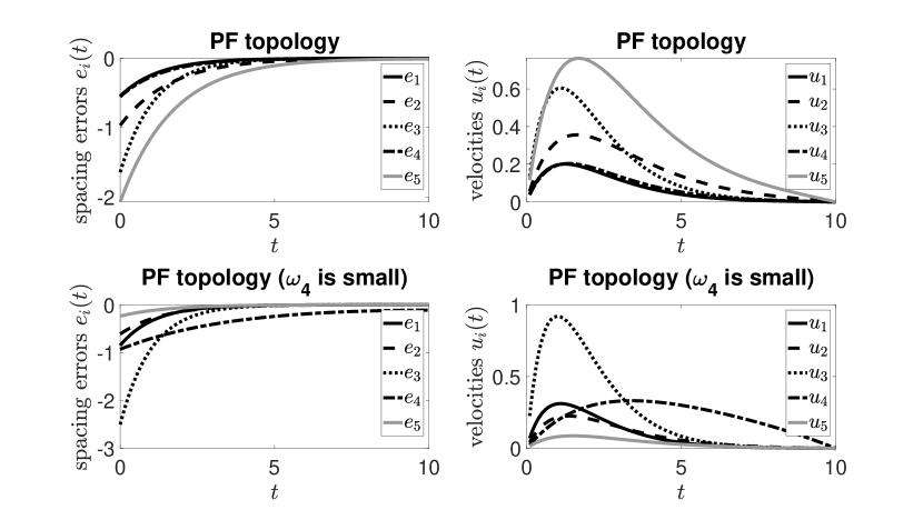
Figure 3: Time histories of relative displacement errors and velocities for the PF topology.

TPF topology: Two experiments were carried out considering the TPF topology. The relevant parameter values are given in Table 2. The time histories of relative displacement errors and velocities corresponding to the first experiment are shown in Figure 4. Compared with time history plots in Figure 3 when the underlying topology is PF, we see that under the TPF topology convergence is faster. In the current experiment, starting from CAV 3 each vehicle receives information from two links that are one sensor link, and one V2V communication link. This accelerates the convergence of the trajectories and velocities.

We run a second experiment to inspect closely the platoon behavior under the TPF topology. In the second experiment, we assume that the CAV 5’s sensor is malfunctioning and this vehicle intends to participate in the platoon and acquire its relative position within the formation only using the V2V communication link (i.e., $\omega_{5}=0$). From Figure 4, we observe that all CAVs, including CAV 5, acquire their predetermined inter-vehicle spacing policies within the specified terminal time.

Table 2: Parameter values for the TPF topology

		Scenario 3				Scenario 4
$i$	$\tilde{\omega}_{i}$	$\omega_{i}$	$d_{i}$	$x_{i}(0)$	$\tilde{\omega}_{i}$	$\omega_{i}$	$d_{i}$	$x_{i}(0)$
0	-	-	-	5.2747	-	-	-	6.4947
1	-	0.9157	-0.1	4.8244	-	0.6948	-0.3	5.7887
2	-	0.7922	-0.3	4.7875	-	0.3171	-0.3	3.7157
3	0.8491	0.9595	-0.2	2.7344	0.3816	0.9502	-0.2	3.2774
4	0.9340	0.6557	-0.1	1.3925	0.7655	0.0344	-0.1	1.9611
5	0.6787	0.0357	-0.3	0.4877	0.7952	0	-0.1	0.8559

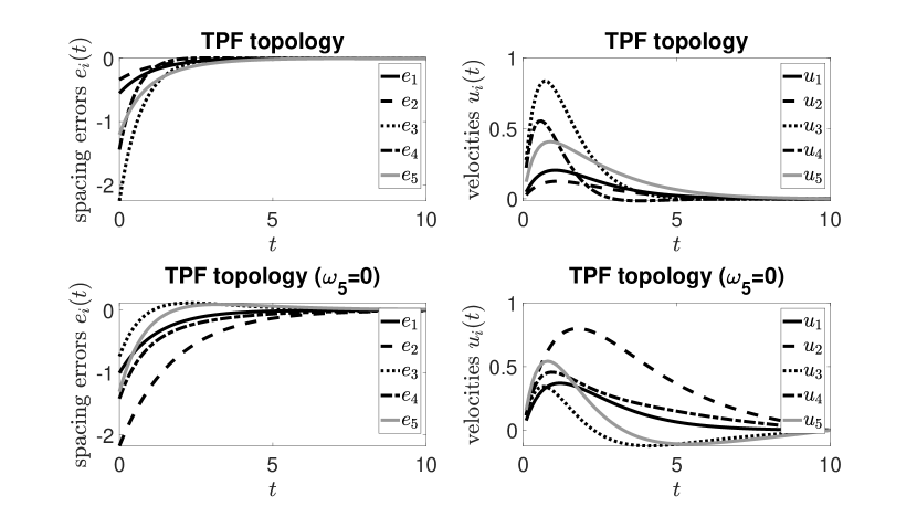
Figure 4: Time histories of relative displacement errors and velocities for the TPF topology.

So far, we have investigated the effectiveness of the models and validated the closed-form solutions for the PF and TPF topologies through relevant experiments. In the following, we run two additional experiments to cover the general topology with the parameter values given in Table 3.

General topology: As two common forms of general communication topologies for a platoon, we consider the All Predecessor Following (APF) and Leader Following (LF) topologies. The time histories of relative displacement errors for these topologies are shown in Figure 5. As it is seen from the figure, the CAVs with the APF topology converge faster while they can not accomplish the predefined inter-vehicle spacing policies exactly with the LF topology in the specified terminal time $t_{f}=10$. This is because of missing the sensor links in the LF topology.

Table 3: Parameter values for the APF and LF topologies

		APF topology				LF topology
$i$	$\mathcal{N}_{i}$	$\omega_{ij}$	$d_{i}$	$x_{i}(0)$	$\mathcal{N}_{i}$	$\omega_{ij}$	$d_{i}$	$x_{i}(0)$
0	-	-	-	5.5166	-	-	-	5.5166
1	{0}	0.6324	-0.2	4.7511	{0}	0.2769	-0.2	4.7511
2	{1}	1.0975	-0.2	2.1937	{1}	0.0462	-0.2	2.1937
3	{1,2}	{0.7547,1.2785}	-0.1	1.9078	{1}	0.0971	-0.1	1.9078
4	{1,2,3}	{0.2760,0.5469,2.9134}	-0.3	1.5855	{1}	0.0935	-0.3	1.5855
5	{1,2,3,4}	{0.9649,0.8147,0.1576,1.9706}	-0.2	0.1722	{1}	0.1948	-0.2	0.1722

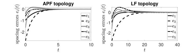
Figure 5: Time histories of relative displacement errors for the APF and LF topologies.

The convergence performance of vehicle platoons is directly related to the algebraic connectivity of their underlying communication topology [37, 53, 54]. In particular, the second-smallest eigenvalue $\sigma_{2}$ (also referred to as the Fiedler value [55]) of the topology Laplacian matrix $\bm{L}$ is a measure of the algebraic connectivity of networked systems. Here, we investigate the influence of the Fiedler value of topology Laplacian matrix and other communication topology-related parameters on the convergence performance of the studied vehicle platoons in the previous experiments. Let’s assume that each trajectory $y_{i}(t)$ convergences when $e_{i}(t)$ falls below the threshold value $0.01$ and let the mean convergence time of all trajectories $y_{i}(t)$ $(i=1,\ldots,n)$ be the convergence performance metric of studied platooning systems. Table 4 shows the Fiedler value, the mean convergence time, the number of communication links, and their mean weight for each platoon system. We observe that in general the higher the Fiedler value the better the convergence performance. The best convergence rate is achieved with the TPF topology where the communication network is better connected and the mean weight is higher compared to other experiments. The worst convergence performance belongs to the LF topology where the corresponding Fiedler value and mean weight are the lowest among all experiments.

Table 4: Topological characteristics of the studied platooning systems

Topology	$\sigma_{i}$	mean time	number of links	mean weight
PF	0.1732	6.8	5	0.5436
PF ($\omega_{4}$ is small)	0.3224	7.9	5	0.5762
TPF	0.5762	3.9	8	0.7276
TPF ($\omega_{5}=0$)	0.3543	8.9	8	0.4923
APF	0.6528	4.1	11	1.0370
LF	0.0199	20.4	5	0.1257

To illustrate the advantage of using the proposed differential game-based platoon control method, we solve two platoon control systems with the PF and TPF topologies using the proposed method and MPC. The parameters of the MPC method are selected as $N=5$ and $T_{s}=0.1$. The platoon parameters for both systems are $n=3$, $t_{f}=15$, $d_{i}=-0.25$ for $i=1,2,3$, and their topologies are defined with the following incidence matrices

$$D_{\text{PF}}=\begin{bmatrix}-1&0&0\\ 1&-1&0\\ 0&1&-1\\ 0&0&1\end{bmatrix},\qquad D_{\text{TPF}}=\begin{bmatrix}-1&0&0&0&\\ 1&-1&0&-1\\ 0&1&-1&0\\ 0&0&1&1\end{bmatrix}.$$

The platoon control systems above using the proposed differential game-based platoon control method easily convert to analytical expressions and closed-form solutions. The associated relative displacement trajectories with the Nash equilibrium are calculated from (14). Once more the relative displacement trajectories using the MPC method are calculated from (83). The time histories of relative displacement errors for these systems with both approaches are shown in Figure 6. It is seen that the proposed control method is cost-effective since each vehicle achieves its relative displacement within the platoon formation by demanding a smaller control effort. Moreover, the MPC is computationally expensive as the underlying optimization repeats at each sampling time.

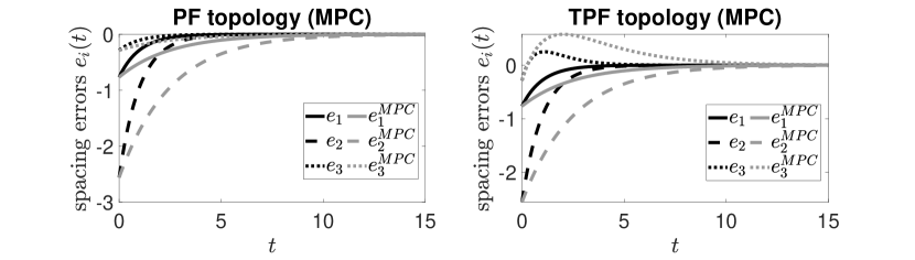
Figure 6: Time histories of relative displacement errors with the proposed control and MPC.

5 Conclusions

In this paper, the CAV platoon formation control is formulated with noncooperative differential games. The existence of a Nash equilibrium controller, which CAVs use as their self-enforcing control strategy to acquire the platoon formation, is proved. Additionally, the CAVs individual relative displacement trajectories are obtained in the closed-form under the PF and TPF topologies and can be calculated numerically under general topology. The simulation studies showed a platoon with 5 vehicles acquired their predetermined inter-vehicle spacing policies utilizing their Nash equilibria. Comparisons with the MPC method have shown that the proposed approach is powerful and promising which enables some future research directions. First, state constraints can be incorporated into the problem. Therefore, the question arises of whether numerical solutions to constrained optimization problems can be obtained. The candidates for such numerical techniques are the Shooting method, Dynamic programming, and the Hamilton-Jacobi-Bellman technique. Another extension is to consider general LTI systems or double integrator dynamics to express the platoon behavior. We might also suppose arbitrary final formation in the optimization problem on top of the unspecified terminal condition utilized in this study. Finally, we can include double states which represent the two-dimensional maneuvers as well. Other possible future directions to address the string-stable platooning control problem are highlighted before.

Acknowledgements

This work was supported by SGS, VSB - Technical University of Ostrava, Czech Republic, under the grant No. SP2022/12 “Parallel processing of Big Data IX”. This work was also supported in part by the Science and Research Council of Turkey (TÜBİTAK) under project EEEAG-121E162.

References

- [1] Soomin Woo and Alexander Skabardonis. Flow-aware platoon formation of connected automated vehicles in a mixed traffic with human-driven vehicles. Transportation Research Part C: Emerging Technologies, 133:103442, 2021.
- [2] Carl Bergenhem, Steven Shladover, Erik Coelingh, Christoffer Englund, and Sadayuki Tsugawa. Overview of platooning systems. In Proceedings of the 19th ITS World Congress, Oct 22-26, Vienna, Austria (2012). ERTICO, 2012.
- [3] Mohammad Y Abualhoul, Mohamed Marouf, Oyunchimeg Shagdar, and Fawzi Nashashibi. Platooning control using visible light communications: A feasibility study. In 16th International IEEE Conference on Intelligent Transportation Systems (ITSC 2013), pages 1535–1540. IEEE, 2013.
- [4] Ziran Wang, Yougang Bian, Steven E Shladover, Guoyuan Wu, Shengbo Eben Li, and Matthew J Barth. Integrated Vehicle-Following Control for Four-Wheel-Independent-Drive Electric Vehicles Against Non-Ideal V2X Communication. IEEE Transactions on Vehicular Technology, 71(4):3648–3659, 2022.
- [5] EL-Zaher Madeleine, Baudouin Dafflon, Franck Gechter, and Jean-Michel Contet. Vehicle platoon control with multi-configuration ability. Procedia Computer Science, 9:1503–1512, 2012.
- [6] William B Dunbar and Derek S Caveney. Distributed receding horizon control of vehicle platoons: Stability and string stability. IEEE Transactions on Automatic Control, 57(3):620–633, 2011.
- [7] Gianluca Antonelli, Filippo Arrichiello, and Stefano Chiaverini. The nsb control: a behavior-based approach for multi-robot systems. Paladyn, Journal of Behavioral Robotics, 1(1):48–56, 2010.
- [8] Wei Ren and Randal W Beard. Decentralized scheme for spacecraft formation flying via the virtual structure approach. Journal of Guidance, Control, and Dynamics, 27(1):73–82, 2004.
- [9] Elham Semsar-Kazerooni, Jan Verhaegh, Jeroen Ploeg, and Mohsen Alirezaei. Cooperative adaptive cruise control: An artificial potential field approach. In 2016 IEEE Intelligent Vehicles Symposium (IV), pages 361–367. IEEE, 2016.
- [10] Ruochen Hao, Meiqi Liu, Wanjing Ma, Bart van Arem, and Meng Wang. A flock-like two-dimensional cooperative vehicle formation model based on potential functions. arXiv preprint arXiv:2104.04153, 2021.
- [11] Lin Li, Ruochen Hao, Wanjing Ma, Xinzhou Qi, and Chenxue Diao. Swarm intelligence based algorithm for management of autonomous vehicles on arterials. Technical report, SAE Technical Paper, USA, 2018.
- [12] Sadayuki Tsugawa. An overview on an automated truck platoon within the energy its project. IFAC Proceedings Volumes, 46(21):41–46, 2013.
- [13] Daniel J Stilwell and Bradley E Bishop. Platoons of underwater vehicles. IEEE Control Systems Magazine, 20(6):45–52, 2000.
- [14] Mo Chen, Qie Hu, Jaime F Fisac, Kene Akametalu, Casey Mackin, and Claire J Tomlin. Reachability-based safety and goal satisfaction of unmanned aerial platoons on air highways. Journal of Guidance, Control, and Dynamics, 40(6):1360–1373, 2017.
- [15] Xiaoling Liang, Chen Xu, and Duansong Wang. Adaptive neural network control for marine surface vehicles platoon with input saturation and output constraints. AIMS Math, 5(1):587–602, 2020.
- [16] Ziran Wang, Yougang Bian, Steven E Shladover, Guoyuan Wu, Shengbo Eben Li, and Matthew J Barth. A survey on cooperative longitudinal motion control of multiple connected and automated vehicles. IEEE Intelligent Transportation Systems Magazine, 12(1):4–24, 2019.
- [17] Serge P Hoogendoorn and Piet Bovy. Generic driving behavior modeling by differential game theory. In Traffic and Granular Flow’07, pages 321–331. Springer, 2009.
- [18] Fabio Morbidi, Patrizio Colaneri, and Thomas Stanger. Decentralized optimal control of a car platoon with guaranteed string stability. In 2013 European Control Conference (ECC), pages 3494–3499. IEEE, 2013.
- [19] Donald E Kirk. Optimal control theory: an introduction. Courier Corporation, 2004.
- [20] Jacob Engwerda. LQ dynamic optimization and differential games. John Wiley & Sons, 2005.
- [21] Cong Wang, Zhenpo Wang, Lei Zhang,Huilong Yu, and Dongpu Cao. Post-Impact Motion Planning and Tracking Control for Autonomous Vehicles. Chinese Journal of Mechanical Engineering, 35–54, 2022.
- [22] Shuyou Yu and Hao Chen and Yangyang Feng and Yajing Zhang and Yongfu Li and Christian Ebenbauer and Hong Chen. Nash optimality based distributed model predictive control for vehicle platoon. IFAC-PapersOnLine, 53(2):6610–6610, 2020.
- [23] Andreas Britzelmeier and Axel Dreves. A decomposition algorithm for Nash equilibria in intersection management. Optimization, 70(11):2441–2478, 2021.
- [24] Peng Hang, Chen Lv, Yang Xing, Chao Huang, Zhongxu Hu. Making for Autonomous Driving: A Noncooperative Game Theoretic Approach. IEEE Transactions on Intelligent Transportation Systems, 22(4):2076–2087, 2021.
- [25] Xiangnan Zhong, Haibo He, Ding Wang, and Zhen Ni. Model-free adaptive control for unknown nonlinear zero-sum differential game. IEEE Transactions on Cybernetics, 48(5):1633–1646, 2017.
- [26] Dongbing Gu. A differential game approach to formation control. IEEE Transactions on Control Systems Technology, 16(1):85–93, 2007.
- [27] Alain Haurie, Jacek B Krawczyk, and Michel Roche. Monitoring cooperative equilibria in a stochastic differential game. Journal of optimization Theory and Applications, 81(1):73–95, 1994.
- [28] Ming Yue, Xiaoqiang Hou, Xudong Zhao, and Xiangmin Wu. Robust Tube-Based Model Predictive Control for Lane Change Maneuver of Tractor-Trailer Vehicles Based on a Polynomial Trajectory. IEEE Transactions on Systems, Man, and Cybernetics: Systems, 50(12): 5180–5188, 2008.
- [29] Tamer Başar and Geert Jan Olsder. Dynamic noncooperative game theory. SIAM, 1998.
- [30] Aykut Yildiz and Hossein B Jond. Vehicle swarm platooning as differential game. In 2021 20th International Conference on Advanced Robotics (ICAR), pages 885–890. IEEE, 2021.
- [31] Ziran Wang, Guoyuan Wu, and Matthew J. Barth. A Review on Cooperative Adaptive Cruise Control (CACC) Systems: Architectures, Controls, and Applications. 2018 21st International Conference on Intelligent Transportation Systems (ITSC), 2884–2891, 2018.
- [32] Shengbo Eben Li, Renjie Li, Jianqiang Wang, Xiaosong Hu, Bo Cheng, Keqiang Li. Stabilizing Periodic Control of Automated Vehicle Platoon With Minimized Fuel Consumption. IEEE Transactions on Transportation Electrification, 3(1): 259–271, 2017.
- [33] Junyan Hu, Parijat Bhowmick, Farshad Arvin, Alexander Lanzon, Barry Lennox. Cooperative Control of Heterogeneous Connected Vehicle Platoons: An Adaptive Leader-Following Approach. IEEE Robotics and Automation Letters, 5(2): 977–984, 2020.
- [34] Yongfu Li, Bangjie Chen, Hang Zhao, Srinivas Peeta, Simon Hu, Yibing Wang, and Zuduo Zheng. A car-following model for connected and automated vehicles with heterogeneous time delays under fixed and switching communication topologies. IEEE Transactions on Intelligent Transportation Systems, pages 1–13, 2021.
- [35] Fu Lin, Makan Fardad, and Mihailo R. Jovanovic. Optimal Control of Vehicular Formations With Nearest Neighbor Interactions. IEEE Transactions on Automatic Control, 57(9): 2203–2218, 2012.
- [36] Myounggyu Won. L-Platooning: A Protocol for Managing a Long Platoon With DSRC. IEEE Transactions on Intelligent Transportation Systems, pages 1–14, 2021.
- [37] Shixi Wen and Ge Guo. Distributed Trajectory Optimization and Sliding Mode Control of Heterogeneous Vehicular Platoons. IEEE Transactions on Intelligent Transportation Systems, pages 1–16, 2021.
- [38] Stephen Andrilli and David Hecker. Chapter 3 - determinants and eigenvalues. In Stephen Andrilli and David Hecker, editors, Elementary Linear Algebra (Fourth Edition), pages 143–202. Academic Press, Boston, fourth edition edition, 2010.
- [39] Dennis S. Bernstein. Matrix Mathematics: Theory, Facts, and Formulas. Princeton University Press, second edition, 2011.
- [40] Shuo Feng, Yi Zhang, Shengbo Eben Li, Zhong Cao, Henry X. Liu, and Li Li. String stability for vehicular platoon control: Definitions and analysis methods. Annual Reviews in Control, 47: 81–97, 2019.
- [41] Yang Zheng, Shengbo Eben Li, Keqiang Li, and Le-Yi Wang. Stability margin improvement of vehicular platoon considering undirected topology and asymmetric control. IEEE Transactions on Control Systems Technology, 24(4): 1253–1265, 2016.
- [42] Yang Zheng, Shengbo Eben Li, Jianqiang Wang, Dongpu Cao, and Keqiang Li. Stability and scalability of homogeneous vehicular platoon: Study on the influence of information flow topologies. IEEE Transactions on Intelligent Transportation Systems, 17(1): 14–26, 2016.
- [43] Reza Olfati-Saber. Flocking for multi-agent dynamic systems: Algorithms and theory. IEEE Transactions on Automatic Control, 51(3): 401–420, 2006.
- [44] Dongbing Gu. A Differential Game Approach to Formation Control. IEEE Transactions on Control Systems Technology, 16(1): 85–93, 2008.
- [45] Hossein B. Jond and Jan Platoš. Autonomous vehicle convoy control as a differential game. preprint arXiv:2101.08858v2, 2021.
- [46] Cong Wang, and Henk Nijmeijer. String Stable Heterogeneous Vehicle Platoon Using Cooperative Adaptive Cruise Control. In 2015 IEEE 18th International Conference on Intelligent Transportation Systems, pages 1977–1982. IEEE, 2015.
- [47] Lingyun Xiao, and Feng Gao. Practical String Stability of Platoon of Adaptive Cruise Control Vehicles. IEEE Transactions on Intelligent Transportation Systems, 12(4): 1184–1194, 2011.
- [48] Muhammad Rony Hidayatullah, and Jyh-Ching Juang. Centralized and Distributed Control Framework Under Homogeneous and Heterogeneous Platoon. IEEE Access, 9: 49629–49648, 2021.
- [49] Sebastian Thormann, Alexander Schirrer, and Stefan Jakubek. Safe and Efficient Cooperative Platooning. IEEE Transactions on Intelligent Transportation Systems, 23(2): 1368–1380, 2022.
- [50] Alexander L. Gratzer, Sebastian Thormann, Alexander Schirrer, Stefan Jakubek. String Stable and Collision-Safe Model Predictive Platoon Control. IEEE Transactions on Intelligent Transportation Systems, 1–16
- [51] Ellen van Nunen, Joey Reinders, Elham Semsar-Kazerooni, Nathan van de Wouw. String Stable Model Predictive Cooperative Adaptive Cruise Control for Heterogeneous Platoons. IEEE Transactions on Intelligent Vehicles, 4(2): 186–196, 2019.
- [52] Pangwei Wang, Hui Deng, Juan Zhang, Li Wang, Mingfang Zhang and Yongfu Li. Model Predictive Control for Connected Vehicle Platoon Under Switching Communication Topology. IEEE Transactions on Intelligent Transportation Systems, 1–14, 2021.
- [53] Qin Xia, Feng Gao, Jianli Duan, Yingdong He. Decoupled H-infinity Control of Automated Vehicular Platoons with Complex Interaction Topologies. IET Intelligent Transport Systems, 11(2): 92–101, 2017.
- [54] Mohammad Pirani, Simone Baldi, and Karl Henrik Johansson. Impact of Network Topology on the Resilience of Vehicle Platoons. IEEE Transactions on Intelligent Transportation Systems, 423(1): 1–12, 2007.
- [55] Nair Maria Maia de Abreu. Old and new results on algebraic connectivity of graphs. Linear Algebra and its Applications, 423(1): 53–73, 2007.