Path eccentricity of graphs

Abstract

Let $G$ be a connected graph. The eccentricity of a path $P$, denoted by $\mathrm{ecc}_{G}(P)$, is the maximum distance from $P$ to any vertex in $G$. In the Central path (CP) problem our aim is to find a path of minimum eccentricity. This problem was introduced by Cockayne et al., in 1981, in the study of different centrality measures on graphs. They showed that CP can be solved in linear time in trees, but it is known to be NP-hard in many classes of graphs such as chordal bipartite graphs, planar 3-connected graphs, split graphs, etc.

We investigate the path eccentricity of a connected graph $G$ as a parameter. Let $\mathrm{pe}(G)$ denote the value of $\mathrm{ecc}_{G}(P)$ for a central path $P$ of $G$. We obtain tight upper bounds for $\mathrm{pe}(G)$ in some graph classes. We show that $\mathrm{pe}(G)\leq 1$ on biconvex graphs and that $\mathrm{pe}(G)\leq 2$ on bipartite convex graphs. Moreover, we design algorithms that find such a path in linear time. On the other hand, by investigating the longest paths of a graph, we obtain tight upper bounds for $\mathrm{pe}(G)$ on general graphs and $k$-connected graphs.

Finally, we study the relation between a central path and a longest path in a graph. We show that on trees, and bipartite permutation graphs, a longest path is also a central path. Furthermore, for superclasses of these graphs, we exhibit counterexamples for this property.

1 Introduction and Preliminaries

For the problem considered here, the input graph is always connected (even if it is not stated explicitly). The length of a path is its number of edges. The distance between two vertices $u$ and $v$ in a graph $G$, denoted by $d_{G}(u,v)$, is the minimum length of a path between them. Moreover, the distance between a vertex $u$ and a set $S\subseteq V(G)$ is $d_{G}(u,S)=\min\{d_{G}(u,v):v\in S\}$.

In the single facility location problem, given a network, one seeks a best site to place a facility in order to serve the other sites of the network. In some applications, we are interested in finding a location that minimizes the maximum distance to the sites. A concept in Graph Theory, related to this measure, is the eccentricity. Let $G$ be a graph. The eccentricity of a vertex $u$, in $G$, is $\max\{d_{G}(u,v):v\in V(G)\}$. A vertex of minimum eccentricity is called a center of $G$. Moreover, the radius of $G$, denoted by $\mathrm{rad}(G)$, is the eccentricity of a center.

A classical generalization for the single facility location problem is the $k$-center problem. In this case, we are interested in finding a set $S$ of $k$ sites, inside a network $G$, that minimizes $\max\{d_{G}(u,S):u\in V(G)\}$. Observe that the places we choose, for those facilities, do not obey any particular structure. When the facilities represent bus stops or train stations, a natural restriction to impose would be the existence of a route (link) between a bus stop and the next one. Thus, the facilities induce a path in the network. This problem is called the Central path (CP) problem. More formally, given a graph $G$, we want to find a path $P$ that minimizes

$$\mathrm{ecc}_{G}(P):=\max\{d_{G}(u,V(P)):u\in V(G)\}.$$

A path that attains this minimum is called a central path of $G$. Cockayne et al. [8] investigated the minimal (regarding vertex-set inclusion) central paths of a graph, and designed a linear-time algorithm for finding such a path on trees. Slater [18] studied central paths of minimum length, and also showed a linear-time algorithm on trees. Observe that a Hamiltonian path is a central path of zero eccentricity. Thus, CP is NP-hard on the classes of graphs for which the Hamiltonian path problem is NP-complete. This is the case for cubic planar $3$-connected graphs [12], split graphs, chordal bipartite graphs [17], etc.

A parameter that is naturally associated with central paths is the path eccentricity of a graph $G$, denoted by $\mathrm{pe}(G)$, and defined as

$$\mathrm{pe}(G):=\min\{ecc_{G}(P):P\text{ is a path in }G\}.$$

We observe that, in a graph $G$, a path $P$ such that $\mathrm{ecc}_{G}(P)\leq\ell$ is also called an $\ell$-dominating path in the literature. Obviously, $G$ has a $\ell$-dominating path if and only if $\mathrm{pe}(G)\leq\ell$.

We start by studying the path eccentricity of convex and biconvex graphs in Section 2. Corneil et. al. [9] showed that if $G$ is an asteroidal triple-free (AT-free) graph, then $\mathrm{pe}(G)\leq 1$. This class of graphs includes interval graphs, permutation graphs, among others. Furthermore, they showed a linear-time algorithm to find such a path. Therefore, in this class of graphs, CP has the same computational complexity as the Hamiltonian path problem. The latter problem is still open on AT-free graphs, however it can be solved in polynomial time in some of its subclasses. Keil [15] showed a linear-time algorithm for the Hamiltonian path problem on interval graphs, and Spinrad et. al. [19] showed and analogous result for bipartite permutation graphs. Therefore, the Central path problem can be solved in linear-time on interval graphs and bipartite permutation graphs.

We extend these results, by studying superclasses of bipartite permutation graphs, such as convex and biconvex graphs, obtaining the following results.

• We can find a 2-dominating path in a convex graph in linear time (Theorem 1). This implies that if $G$ is a convex graph, then $\mathrm{pe}(G)\leq 2$ (Corollary 1). Moreover, this bound is tight.

• We can find a dominating path in a biconvex graph in linear time (Theorem 3). This implies that if $G$ is a biconvex graph, then $\mathrm{pe}(G)\leq 1$ (Corollary 3). Moreover, this bound is tight.

In Section 3, we investigate upper bounds for $\mathrm{pe}(G)$ on general graphs and on $k$-connected graphs. Since a single vertex can be regarded as a path of length zero, any upper bound for the radius of a graph is also valid for $\mathrm{pe}(G)$. Let $n$ denote the order of a graph $G$. In 1987, Erdős et al. [10] showed that the radius of $G$ is at most $(3n-5)/(2\delta(G)+1)+5$. If $G$ is $3$-connected, Harant [14] showed an upper bound of $n/4+8$ for the radius of $G$. Hence these are valid bounds for $\mathrm{pe}(G)$ for connected and 3-connected graphs. We improve these results by proving the following.

• For every connected graph $G$ on $n$ vertices, we have $\mathrm{pe}(G)\leq\frac{n-1}{3}$. Moreover, this bound is tight (Theorem 4).

• For every $k$-connected graph $G$ on $n$ vertices, with $k\geq 2$, we have $\mathrm{pe}(G)\leq\frac{n+k}{3k+2}$. Moreover, this bound is tight (Theorem 5).

The previous tight upper bounds for $\mathrm{pe}(G)$ were obtaining by studying the eccentricity of longest paths. So, a natural question is whether a longest path is always a central path. We investigate the relationship between central paths and longest paths in Section 4. We show that

• In trees, $4$-connected planar graphs, proper interval graphs, and bipartite permutation graphs, every longest path is a central path (Corollaries 6, 7, and 8).

• On the other hand, on cacti, $2$-connected planar graphs, interval graphs and convex graphs, it is not always the case that every longest path is a central path (Figures 5, 6, and 7) .

Finally, we discuss some open problems and give concluding remarks in Section 5.

To conclude this section, we give a simple observation, used throughout the text, to derive families of graphs that exhibit a tight upper bound for $\mathrm{pe}(G)$. Let $G$ be a graph. Let us denote by $\mathcal{C}(G)$ the collection of components in $G$.

Proposition 1

Let $G$ be a connected graph. Let $S\subseteq V(G)$ such that $|\mathcal{C}(G-S)|\geq|S|+2$. Then,

$$\mathrm{pe}(G)\geq\min\{\mathrm{ecc}_{G}(S,C):C\in\mathcal{C}(G-S)\},$$

where $\mathrm{ecc}_{G}(S,C):=\max\{d_{G}(u,S):u\in V(C)\}$.

Proof 1

Let $P$ be a central path of $G$. Note that $P-S$ has at most $|S|+1$ components. As $|\mathcal{C}(G-S)|\geq|S|+2$, there exists a component $C^{*}\in\mathcal{C}(G-S)$ such that $V(P)\cap V(C^{*})=\emptyset$. Thus, any path between $V(P)$ and $V(C^{*})$ contains a vertex in $S$. This implies that

$$\mathrm{pe}(G)=\mathrm{ecc}_{G}(P)\geq d_{G}(u,V(P))\geq d_{G}(u,S)+d_{G}(S,V(P))\geq d_{G}(u,S),$$

for any vertex $u\in V(C^{*})$. Therefore, $\mathrm{pe}(G)\geq\mathrm{ecc}(S,C^{*})$.

2 Path eccentricity of convex graphs and subclasses

As mentioned in the previous section, bipartite permutation graphs have bounded path eccentricity. In this section, we seek to extend this result studying classes of graphs, such as convex and biconvex graphs, that properly contain the bipartite permutation graphs. Moreover, we show that these classes also have bounded path eccentricity.

2.1 Convex graphs

Let $G=(X\cup Y,E)$ be a bipartite graph. We say that $G$ is $X$-convex if there is an ordering of the vertices in $X$, such that $N_{G}(y)$ consists of consecutive vertices in that ordering, for each $y\in Y$. We call such ordering a convex ordering of $X$. If $G$ is an $X$-convex graph, we abbreviate this fact saying that $G$ is convex. In what follows, $G$ denotes a convex graph, and we consider that $\{x_{1},x_{2},\ldots,x_{n}\}$ is a convex ordering of $X$. Moreover, we say that $x_{i}<x_{j}$ if $i<j$; and for each vertex $y\in Y$, we define

$$\begin{array}[]{rcl}\ell(y)&:=&\min\{x:x\in N_{G}(y)\},\text{ and}\\ r(y)&:=&\max\{x:x\in N_{G}(y)\}.\end{array}$$

Algorithm 1 finds a $2$-dominating path, say $P$, of $G$ greedily. Starting with $P=\langle a_{1}\rangle$, where $a_{1}=x_{1}$, we extend $P$ by appending a vertex $y$, in $N_{G}(a_{1})$, that maximizes $r(y)$. After that, we also append $a_{2}=r(y)$ to $P$ and repeat this procedure until the last vertex in the path is $x_{n}$.

Algorithm 1 2Dom-Path-Convex$(G)$

Input: A connected convex graph $G=(X\cup Y,E)$
Output: A $2$-dominating path of $G$

1:Find a convex ordering of $X$, say $\{x_{1},x_{2},\ldots,x_{n}\}$

2:$a_{1}\leftarrow x_{1}$

3:$k\leftarrow 1$

4:while $a_{k}\neq x_{n}$ :

5:     $b_{k}\leftarrow\operatorname*{arg\,max}\{r(y):y\in N_{G}(a_{k})\}$

6:     $a_{k+1}\leftarrow r(b_{k})$

7:     $k\leftarrow k+1$

8:return $\langle a_{1},b_{1},\ldots,b_{k-1},a_{k}\rangle$

Theorem 1

Algorithm 1 finds a $2$-dominating path in a convex graph $G$ in $\mathcal{O}(|V(G)|+|E(G)|)$ time.

Proof 2

First, we show that the loop of lines 4-7 terminates. For this, we show that if $a_{k}\neq x_{n}$ (at any iteration) then

$$a_{k}<\max\{r(y):y\in N_{G}(a_{k})\}.$$

That is, at line 6, we have $a_{k}<a_{k+1}$. Let $X_{1}=\{x:x\in X,\,x\leq a_{k}\}$ and $Y_{1}=N_{G}(X_{1})$. Let $X_{2}$ (resp. $Y_{2}$) be $X\setminus X_{1}$ (resp. $Y\setminus Y_{1}$). Let $G_{1}$ (resp. $G_{2}$) be the graph induced by $X_{1}\cup Y_{1}$ (resp. $X_{2}\cup Y_{2}$). Since $G$ is connected and $G_{2}$ contains $x_{n}$, then there must exist an edge linking $G_{1}$ to $G_{2}$. Now, by the definition of $Y_{1}$, there is no edge between $X_{1}$ and $Y_{2}$. Thus, the edge linking $G_{1}$ to $G_{2}$ must be between a vertex $y^{*}\in Y_{1}$ and vertex in $X_{2}$. The convexity of $X$ implies that $\ell(y^{*})\leq a_{k}<r(y^{*})$, and thus $y^{*}\in N_{G}(a_{k})$. Therefore, we have $a_{k}<r(y^{*})\leq a_{k+1}$.

Let $k^{*}$ be the value of $k$ at the end of the algorithm. By the previous arguments $a_{k^{*}}=x_{n}$. Now, we show that $P=\langle a_{1},b_{1},\ldots,b_{k^{*}-1},a_{k^{*}}\rangle$ is a $2$-dominating path of $G$. Since $b_{i}$ is adjacent to $a_{i}$ and $a_{i+1}$, convexity implies that

$$\bigcup_{i=1}^{k^{*}-1}{N_{G}(b_{i})}=X.$$

Thus, it suffices to show that every vertex in $Y$ is at distance at most two from a vertex in $P$. Let $y\in Y$. Since $a_{1}=x_{1}$ and $a_{k^{*}}=x_{n}$, then $a_{i}\leq\ell(y)\leq a_{i+1}$, for some $1\leq i<k^{*}$. Moreover, as $b_{i}$ is adjacent to $a_{i}$ and $a_{i+1}$, the vertex $b_{i}$ must be adjacent to $\ell(y)$ by convexity. Thus, $y$ is at distance at most two from $P$. Regarding the time complexity of the algorithm, the ordering at line 1 is computed in linear time [4]. Finally, the loop of lines 4-7 runs in $\mathcal{O}(|V(G)|+|E(G)|)$ time. Therefore, Algorithm 1 runs in $\mathcal{O}(|V(G)|+|E(G)|)$ time.

The previous theorem implies the following upper bound on $\mathrm{pe}(G)$.

Corollary 1

If $G$ is a convex graph, then $\mathrm{pe}(G)\leq 2$.

Now, we show that this bound is tight. Furthermore, we show that for every positive integer $k$, there exists a $k$-connected convex graph that attains this bound. Let $k$ be a positive integer, and let $\ell:=k(k+2)$. Let $K_{k,\ell}$ be the complete bipartite graph with one side of size $k$ and the other side of size $\ell$. Since $\ell>k$, then $K_{k,\ell}$ is a $k$-connected graph. In what follows, we consider that $K_{k,\ell}$ is a $(X,Y)$-bipartite graph such that $|X|=\ell$, $|Y|=k$ and

$$X=\{x_{1},x_{2},\ldots,x_{\ell}\}.$$

We observe that $K_{k,\ell}$ is $X$-convex. Let $G$ be the graph defined as follows:

$$\begin{array}[]{rcl}V(G)&=&V(K_{k,\ell})\cup\{z_{i}:1\leq i\leq k+2\},\\ E(G)&=&E(K_{k,\ell})\cup\{z_{i}x_{j}:1\leq i\leq k+2,\,(i-1)\cdot k+1\leq j\leq i\cdot k\}.\end{array}$$

Since each vertex $z_{i}$ is adjacent to $k$ vertices in $X$, and $K_{k,\ell}$ is bipartite $k$-connected, we have that $G$ is also bipartite $k$-connected. Furthermore, as $N_{G}(z_{i})=\{x_{j}\in X:(i-1)\cdot k+1\leq j\leq i\cdot k\}$, $G$ is also $X$-convex. Finally, if we consider $S=Y$, then each component $C$ in $\mathcal{C}(G-S)$ is a star such that its center is the unique vertex, in $C$, not adjacent to $S$. Thus, $\mathrm{ecc}_{G}(S,C)=2$, for each $C\in\mathcal{C}(G-S)$. By Proposition 1 and Corollary 1, we have that $\mathrm{pe}(G)=2$. We show an example of this construction for $k=2$ in Figure 1.

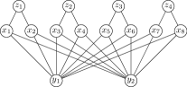
Figure 1: A convex $2$-connected graph $G$ such that $\mathrm{pe}(G)=2$.

2.2 Biconvex graphs

In this section we study the parameter $\mathrm{pe}(G)$ on biconvex graphs (a subclass of convex graphs), and improve the result obtained in the previous section. We show that $\mathrm{pe}(G)\leq 1$ for every biconvex graph $G$. We say that a $(X,Y)$-bipartite graph is biconvex if it is both, $X$-convex and $Y$-convex. Moreover, we say that $V(G)=X\cup Y$ admits a biconvex ordering. A subclass of biconvex graphs are the bipartite permutation graphs. A result of Corneil et. al. [9] implies that bipartite permutation graphs admit a dominating path. For ease of explanation, we will show an algorithm that finds such a path on bipartite permutation graphs. After that, we modify this algorithm in order to find a dominating path in any biconvex graph $G$ (implying that $\mathrm{pe}(G)\leq 1$).

Let $G=(X\cup Y,E)$ be a connected bipartite permutation graph. Spinrad et al. [19] (see Theorem 1) showed that $V(G)$ admits a biconvex ordering, say $X=\{x_{1},\ldots,x_{n}\}$ and $Y=\{y_{1},\ldots,y_{m}\}$, that satisfy one additional property. Let $u$ and $v$ be two vertices in the same part of $G$. If $u$ comes before $v$ in the previous ordering, we write $u<v$ to indicate this fact. Consider $x_{i},x_{k}\in X$ and $y_{a},y_{c}\in Y$ such that $x_{i}\leq x_{k}$ and $y_{a}\leq y_{c}$. Then, we have the following:

1. if $x_{i}y_{c}$ and $x_{k}y_{a}$ belong to $E$, then $x_{i}y_{a}$ and $x_{k}y_{c}$ also belong to $E$.

An ordering of $V(G)$ that satisfies $(\star)$ is called strong. Yu & Chen [23] (see Lemma 7) noted that every strong ordering of $V(G)$ is also biconvex. The main tool that we use to construct a dominating path in $G$ is a decomposition of $V(G)$ showed by Uehara & Valiente [22]. They showed that, given a strong ordering of $V(G)$, we can decompose $G$ into subgraphs $(K_{1}\cup J_{1}),\ldots,(K_{k}\cup J_{k})$ in the following way. First, let $K_{1}$ be the graph induced by $N(x_{1})\cup N(y_{1})$. Let $J_{1}$ be the set of isolated vertices (maybe empty) in $G-K_{1}$. Now, consider that $G=G-(K_{1}\cup J_{1})$, and repeat this process until the graph becomes empty. They called this decomposition a complete bipartite decomposition of $G$. Moreover, they showed that it can be obtained in $\mathcal{O}(|V(G)|)$. Let $\ell_{X}(K_{i})$ and $r_{X}(K_{i})$ be the vertices in $V(K_{i})\cap X$ such that

$$\begin{array}[]{rl}\ell_{X}(K_{i})\leq x,\text{ for each }x\in V(K_{i})\cap X,\\ r_{X}(K_{i})\geq x,\text{ for each }x\in V(K_{i})\cap X.\\ \end{array}$$

In a similar way, we define $\ell_{Y}(K_{i})$ and $r_{Y}(K_{i})$, for $i=1,\ldots,k$. Observe that,

$$V(K_{i})=N_{G}(\ell_{X}(K_{i}))\cup N_{G}(\ell_{Y}(K_{i})),\,\text{for }i=1,\ldots,k.$$

In what follows, we say that two sets of vertices are adjacent if there exists an edge linking them. Uehara & Valiente [22] showed that this decomposition satisfies the following properties:

1. $K_{i}$ is a nontrivial (with at least one edge) complete bipartite graph. Moreover, $V(K_{i})$ is adjacent to $V(K_{i+1})$, but not to $V(K_{\ell})$, for $\ell>i+1$.

2. For each $i\in\{1,\ldots,k\}$, either $J_{i}\subseteq X$ or $J_{i}\subseteq Y$.

3. For each $i\in\{1,\ldots,k\}$, if $J_{i}\subseteq X$ (resp. $J_{i}\subseteq Y$), then $J_{i}$ is a continuous sequence of vertices in the ordering of $X$ (resp. $Y$). Furthermore, $r_{X}(K_{i})\leq a\leq\ell_{X}(K_{i+1})$ (resp. $r_{Y}(K_{i})\leq a\leq\ell_{Y}(K_{i+1})$), for each $a\in J_{i}$.

4. $N_{G}(J_{i})\subseteq V(K_{i})$, for $1\leq i\leq k$. Furthermore, if $a,a^{\prime}\in J_{i}$ and $a\leq a^{\prime}$, then $N_{G}(a^{\prime})\subseteq N_{G}(a)$.

Let $e$ be an edge with one end in $K_{i}$ and the other in $K_{i+1}$. We say that $e$ is an $XY$-edge if the end of $e$, in $K_{i}$, belongs to $X$. In an analogous way, we define a $YX$-edge. The idea of our algorithm is to construct a dominating path of $G$ incrementally. Given a dominating path $P$ of the graph induced by $(K_{1}\cup J_{1})\cup\ldots\cup(K_{i}\cup J_{i})$, at the $i$-th step, we extend $P$ to dominate $(K_{i+1}\cup J_{i+1})$. In particular, the following three properties will be used to show the correctness of our algorithm.

1. If $K_{i}$ is linked to $K_{i+1}$ with an $XY$-edge (resp. a $YX$-edge), then $r_{X}(K_{i})$ (resp. $r_{Y}(K_{i})$) is adjacent to $\ell_{Y}(K_{i+1})$ (resp. $\ell_{X}(K_{i+1})$).

2. If $J_{i}\subseteq Y$ (resp. $J_{i}\subseteq X$), then $r_{X}(K_{i})\in N(v)$ (resp. $r_{Y}(K_{i})\in N(v)$), for every $v\in J_{i}$.

3. If $K_{i}$ is linked to $K_{i+1}$ by an $XY$-edge and a $YX$-edge, then $J_{i}=\emptyset$.

We observe that $\ref{prop:extra1})$ follows from the convexity of the orderings of $X$ and $Y$. Moreover, both $\ref{prop:extra2})$ and $\ref{prop:extra3})$ follow from $\ref{prop:Ji})$ and $\ref{prop:inK})$ using the fact that the vertex ordering is biconvex and strong. Let $P=\langle a_{1},\ldots,a_{n}\rangle$ and $Q=\langle b_{1},\ldots,b_{m}\rangle$ be vertex-disjoint paths, in $G$, such that $a_{n}$ is adjacent to $b_{1}$. Then, the concatenation of $P$ and $Q$, denoted by $P\cdot Q$, is the path $\langle a_{1},\ldots,a_{n},b_{1},\ldots,b_{m}\rangle$. Now, we present Algorithm 2 that finds a dominating path in bipartite permutation graphs.

Algorithm 2 Dom-Path-BPG$(G)$

Input: A connected bipartite permutation graph $G=(X\cup Y,E)$
Output: A dominating path $P$ of $G$

1:Find a strong convex ordering of $X$ and $Y$, say $\{x_{1},\ldots,x_{n}\}$ and $\{y_{1},\ldots,y_{m}\}$

2:Let $(K_{1},J_{1}),\ldots,(K_{k},J_{k})$ be a complete bipartite decomposition of $G$

3:$P\leftarrow\emptyset$

4:$v\leftarrow\ell_{X}(K_{1})$

5:for $i\leftarrow 1$ to $k-1$ :

6:     if $K_{i}$ is linked to $K_{i+1}$ by an $XY$-edge :

7:         Let $P^{\prime}$ be a path between $v$ and $r_{X}(K_{i})$

8:         $v\leftarrow\ell_{Y}(K_{i+1})$

9:     else

10:         Let $P^{\prime}$ be a path between $v$ and $r_{Y}(K_{i})$

11:         $v\leftarrow\ell_{X}(K_{i+1})$      

12:     $P\leftarrow P\cdot P^{\prime}$

13:if $J_{k}\subseteq Y$ :

14:     Let $P^{\prime}$ be a path between $v$ and $r_{X}(K_{k})$

15:else

16:     Let $P^{\prime}$ be a path between $v$ and $r_{Y}(K_{k})$

17:$P\leftarrow P\cdot P^{\prime}$

18:return $P$

Theorem 2

Algorithm 2 finds a dominating path in a bipartite permutation graph $G$ in $\mathcal{O}(|V(G)|+|E(G)|)$.

Proof 3

First, we show that the algorithm correctly constructs a path $P$. Note that lines 4, 8, and 11 imply that the variable $v$ represents either $\ell_{X}(K_{i})$ or $\ell_{Y}(K_{i})$ at the beginning of each iteration of the loop at lines 5-12. Since $K_{i}$ is complete bipartite, there is always a path between $v$ and $r_{X}(K_{i})$ or $r_{Y}(K_{i})$. Furthermore, by e), $r_{X}(K_{i})$ (resp. $r_{Y}(K_{i})$) is adjacent to $\ell_{Y}(K_{i+1})$ (resp. $\ell_{X}(K_{i+1})$) when there exists an $XY$-edge (resp. a $YX$-edge) between $K_{i}$ and $K_{i+1}$. Therefore, Algorithm 2 returns a path.

Now, we show that $P$ is a dominating path. First, we prove that $P$ dominates $V(K_{i})$, for $i=1,\ldots,k$. Observe that, if $K_{i}\cong K_{n,m}$ where $n,m\geq 2$, then any path between $v$ and $r_{X}(K_{i})$ or $r_{Y}(K_{i})$ must contain an edge of $K_{i}$. Thus, $P$ dominates $V(K_{i})$. Now, suppose that $K_{i}\cong K_{1,m}$ for $m\geq 1$. Without loss of generality, suppose that $\ell_{X}(K_{i})=r_{X}(K_{i})$ (a center of the star $K_{1,m}$). Observe that, either if $v=\ell_{X}(K_{i})$ or $v=\ell_{Y}(K_{i})$, the path $P^{\prime}$ (at lines 7, 10, 14, 16) will contain a center of $K_{1,m}$. Therefore, $P$ dominates every $K_{i}$.

Finally, we show that $P$ dominates every $J_{i}$, for $i=1,\ldots,k$. For this, we show that $P$ contains $r_{X}(K_{i})$ if $J_{i}\subseteq Y$, otherwise it contains $r_{Y}(K_{i})$. Let $J_{i}\neq\emptyset$ such that $i<k$. Then, by $\ref{prop:extra3})$, $K_{i}$ is linked to $K_{i+1}$ either by $XY$-edges or $YX$-edges. Without loss of generality, suppose that there exists an $XY$-edge, say $xy\in E(G)$, between $K_{i}$ and $K_{i+1}$. Then, line 7 implies that $P$ contains $r_{X}(K_{i})$. Thus, by $\ref{prop:extra2})$, $P$ dominates $J_{i}$. Finally, lines 14 and 16 ensure that $P$ dominates $J_{k}$.

Regarding the computational complexity of the algorithm, line 1 is computed in $\mathcal{O}(|V(G)|+|E(G)|)$ time [19]. Moreover, the complete bipartite decomposition of $G$ is computed in $\mathcal{O}(|V(G)|)$ time [22]. To conclude, the paths at lines 7, 10, 14 and 16 are computed in constant time, as each $K_{i}$ is complete bipartite. Therefore, the complexity of Algorithm 2 is $\mathcal{O}(|V(G)|+|E(G)|)$.

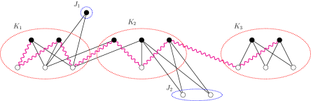
Figure 2: A dominating path found by Algorithm 2 on a bipartite permutation graph.

In Figure 2, we show a bipartite permutation graph. The set $X$ (resp. $Y$) is represented by the black (resp. white) vertices, and a dominating path found by Algorithm 2 is represented by the wavy edges. In what follows, we show how to modify Algorithm 2 in order to find a dominating path in a biconvex graph. For this, we use a result of Yu & Chen [23] which states that every biconvex graph contains a bipartite permutation graph as an induced subgraph. Let $G=(X\cup Y,E)$ be a biconvex graph such that $X=\{x_{1},\ldots,x_{n}\}$ and $Y=\{y_{1},\ldots,y_{m}\}$ represent a biconvex ordering of $X\cup Y$. Let $x_{L}$ (resp. $x_{R}$) be the vertex in $N(y_{1})$ (resp. $N(y_{m})$) such that $N(x_{L})$ (resp. $N(x_{R})$) is not properly contained in any other neighborhood set. In case of ties, we choose $x_{L}$ (resp. $x_{R}$) to be the smallest (resp. largest) index vertex. Observe that, we may assume that $x_{L}\leq x_{R}$, otherwise we can consider the reverse ordering of $X$. Now, let $X_{p}=\{x_{i}:x_{L}\leq x\leq x_{R}\}$, and let $G_{p}=G[X_{p}\cup Y]$. Yu & Chen [23] showed the following.

Lemma 1 (Yu & Chen, 1995)

$G_{p}$ is a bipartite permutation graph.

Moreover, Abbas & Stewart [1] showed further properties of $X-X_{p}$.

Lemma 2 (Abbas & Stewart, 2000)

Let $G=(X\cup Y,E)$ be a biconvex graph. There exists an ordering of $V(G)$, say $X=\{x_{1},\ldots,x_{n}\}$ and $Y=\{y_{1},\ldots,y_{m}\}$, such that the following hold:

1. $G_{p}$ is a bipartite permutation graph.

2. $X_{p}=\{x_{L},x_{L+1},\ldots,x_{R}\}$ and $Y=\{y_{1},y_{2},\ldots,y_{m}\}$ is a strong ordering of $V(G_{p})$.

3. For all $x_{i}$ and $x_{j}$, where $x_{1}\leq x_{i}<x_{j}\leq x_{L}$ or $x_{R}\leq x_{j}<x_{i}\leq x_{n}$, then $N(x_{i})\subseteq N(x_{j})$.

Our aim is to use the above lemma to find a dominating path on a biconvex graph. As $G_{p}$ is a bipartite permutation graph, it has a complete bipartite decomposition, say $(K_{1},J_{1}),\ldots,(K_{k},J_{k})$. Furthermore, observe that $x_{L}=\ell_{X}(K_{1})$ and $x_{R}\in\{r_{X}(K_{k})\}\cup J_{k}$. Thus, by Lemma 2 $\ref{it:important})$, we have the following.

Corollary 2

Let $G_{p}$ be the bipartite permutation graph defined from $G$, and let $(K_{1},J_{1}),\ldots,(K_{k},J_{k})$ be its complete bipartite decomposition. Then,

$$\begin{array}[]{rl}N(x_{i})\subseteq V(K_{1}),&\text{for }i=1,2,\ldots,L,\\ N(x_{j})\subseteq V(K_{k})\cup J_{k},&\text{for }j=R,R+1,\ldots,n.\\ \end{array}$$

The previous result implies that, to obtain a dominating path of $G$, we need to carefully choose the vertices in $(V(K_{1})\cup\{x_{1},\ldots,x_{L-1}\})$ and $(V(K_{k})\cup J_{k}\cup\{x_{R+1},\ldots,x_{n}\})$ that belong to the path. Algorithm 3 finds a dominating path in a biconvex graph. The line 10 of Algorithm 3 represents the loop of lines 5-12 of Algorithm 2. We recall the following property of a complete bipartite decomposition of $G_{p}$. We will use it to show the correctness of our algorithm.

1. If $J_{i}\subseteq Y$ (resp. $J_{i}\subseteq X$), then $r_{X}(K_{i})\in N(v)$ (resp. $r_{Y}(K_{i})\in N(v)$), for every $v\in J_{i}$.

Algorithm 3 Dominating-Path-Biconvex$(G)$

Input: A connected biconvex graph $G=(X\cup Y,E)$
Output: A dominating path $P$ of $G$

1:Find a biconvex ordering $\{x_{1},\ldots,x_{n}\}$ and $\{y_{1},\ldots,y_{m}\}$ that satisfy Lemma 2

2:Let $G_{p}$ be the graph induced by $\{x_{L},\ldots,x_{R}\}\cup Y$

3:Let $(K_{1},J_{1}),\ldots,(K_{k},J_{k})$ be the complete bipartite decomposition of $G_{p}$

4:if $r_{Y}(K_{1})\in N_{G}(x_{1})$ :

5:     $P\leftarrow\langle\ell_{X}(K_{1})\rangle$

6:     $v\leftarrow r_{Y}(K_{1})$

7:else

8:     $P\leftarrow\emptyset$

9:     $v\leftarrow\min\{y_{j}:y_{j}\in N_{G}(x_{1})\}$

10:Process $(K_{1}\cup J_{1}),\ldots,(K_{k-1}\cup J_{k-1})$

11:Let $P^{\prime}$ be a path between $v$ and $r_{X}(K_{k})$

12:if $N_{G}(x_{n})\cap J_{k}\neq\emptyset$ :

13:     Let $u$ be a vertex in $N_{G}(x_{n})\cap J_{k}$

14:     $P^{\prime}\leftarrow P^{\prime}\cdot\langle u\rangle$

15:else

16:     if $V(P^{\prime})\cap N_{G}(x_{n})=\emptyset$ :

17:         Let $u$ be a vertex in $N_{G}(x_{n})$

18:         $P^{\prime}\leftarrow P^{\prime}\cdot\langle u\rangle$      

19:$P\leftarrow P\cdot P^{\prime}$

20:return $P$

Theorem 3

Algorithm 3 finds a dominating path in a connected biconvex graph $G$.

Proof 4

By the proof of Theorem 2, $P$ dominates $J_{1}$ and $(K_{i}\cup J_{i})$, for $i=2,\ldots,k-1$. In what follows, we show that $P$ dominates $A=V(K_{1})\cup\{x_{1},\ldots,x_{L-1}\}$. First, suppose that $r_{Y}(K_{1})\in N_{G}(x_{1})$. By Lemma 2 c), the vertex $r_{Y}(K_{1})$ dominates $x_{i}$, for $x_{1}\leq x_{i}\leq x_{L-1}$. Moreover, since $\{\ell_{X}(K_{1}),r_{Y}(K_{1})\}$ dominates $K_{1}$, the path $P$ dominates $A$. Now, suppose that $r_{Y}(K_{1})\notin N_{G}(x_{1})$, and let $y^{*}=\min\{y_{j}:y_{j}\in N_{G}(x_{1})\}$. Since $y^{*}<r_{Y}(K_{1})$, any path from $y^{*}$ to either $r_{X}(K_{1})$ or $r_{Y}(K_{1})$ must contain a vertex in $V(K_{1})\cap X$. Thus, $P$ contains a vertex $x^{*}\in V(K_{1})\cap X$. By similar arguments as before, the set $\{x^{*},y^{*}\}\subseteq V(P)$ dominates $A$.

Finally, we show that $P$ dominates $B=K_{k}\cup J_{k}\cup\{x_{R+1},\ldots,x_{n}\}$. Consider the variable $v$ after the execution of line 10. Note that if either $v=\ell_{X}(K_{k})$ or $v=\ell_{Y}(K_{k})$, the path $P^{\prime}$ in line 11 dominates $V(K_{k})$. Now, we show that $P$ dominates $J_{k}\cup\{x_{R+1},\ldots,x_{n}\}$. We distinguish two cases.

Case 1: $N_{G}(x_{n})\cap J_{k}\neq\emptyset$.

In this case $J_{k}\subseteq Y$. By $\ref{prop:extra2})$, every vertex in $J_{k}$ is adjacent to $r_{X}(K_{k})$, and thus, $P$ dominates $J_{k}$. Furthermore, by Lemma 2 c), the vertex $u$ (at line 13) dominates $x_{i}$, for $x_{R+1}\leq x_{i}\leq x_{n}$. Therefore, $P$ dominates $B$.

Case 2: $N_{G}(x_{n})\cap J_{k}=\emptyset$.

In this case $N_{G}(x_{n})\subseteq V(K_{k})$. If $V(P^{\prime})\cap N_{G}(x_{n})\neq\emptyset$, Lemma 2 $\ref{it:important})$ implies that $P$ dominates $B$. So, suppose that $V(P^{\prime})\cap N_{G}(x_{n})=\emptyset$. Then, the vertex $u\in N_{G}(x_{n})$ at line 17 is adjacent to $r_{X}(K_{k})$, and Lemma 2 $\ref{it:important})$ implies that $P$ dominates $x_{i}$, for $x_{R+1}\leq x_{i}\leq x_{n}$. Now, we show that $P$ dominates $J_{k}$. If $J_{k}\subseteq Y$, by $\ref{prop:extra2})$, the vertex $r_{X}(K_{k})$ dominates $J_{k}$. Otherwise, suppose that $J_{k}\subseteq X$. Let $x$ be any vertex in $J_{k}$, we will show that $u$ dominates $x$. Observe that the vertices $u$, $r_{Y}(K_{k})$, $x$ and $x_{R}$ belong to $G_{p}$. Moreover, as $u\in V(K_{k})$, we have that $u\leq r_{Y}(K_{k})$. By definition of $G_{p}$, we also have that $x\leq x_{R}$. Observe that, by Lemma 2 c), $u$ is adjacent to $x_{R}$. Furthermore, by $\ref{prop:extra2})$, the vertex $r_{Y}(K_{k})$ is adjacent to $x$. Thus, since the ordering of $V(G_{p})$ is strong, $x$ is adjacent to $u$. Therefore, $P$ dominates $B$.

The previous theorem implies the following result.

Corollary 3

If $G$ is a biconvex graph, then $\mathrm{pe}(G)\leq 1$.

To conclude, we observe that this bound is tight even if $G$ is $k$-connected. For this, consider the complete bipartite graph $K_{k,k+2}$. Observe that $K_{k,k+2}$ is $k$-connected and also biconvex. Moreover, by Proposition 1, we have $\mathrm{pe}(K_{k,k+2})=1$.

3 Upper bounds for $\mathrm{pe}(G)$ in general and $k$-connected graphs

In this section, we show an upper bound for $\mathrm{pe}(G)$ when $G$ is a general (and connected) graph, and when $G$ is $k$-connected with $k\geq 2$. Given a path $P$ and two vertices $x$ and $y$ in $P$, we denote by $P[x,y]$ the subpath of $P$ with extremes $x$ and $y$. Note that $d_{P}(x,y)=|P[x,y]|$. We begin by showing a result for any connected graph. Recall that $\mathrm{ecc}_{G}(P)=\max\{d_{G}(u,V(P)):u\in V(G)\}$ and $\mathrm{pe}(G)=\min\{\mathrm{ecc}_{G}(P):~{}P\text{ is a path in }G\}$.

Theorem 4

For any connected graph $G$ on $n$ vertices, $\mathrm{pe}(G)\leq\frac{n-1}{3}$. Moreover, this bound is tight.

Proof 5

Let $P$ be a longest path of $G$ with length $L$. Let $v$ be a vertex of $G$ with $d_{G}(v,V(P))=\mathrm{ecc}_{G}(P)$, and let $Q$ be a shortest path from $v$ to $P$. Then, as $|V(P)\cup V(Q)|\leq n$, we have

$$|Q|\leq n-L-1.$$ (1)

Also, as $P$ is a longest path, we have

$$|Q|\leq L/2.$$ (2)

Indeed, otherwise we can join $Q$ with a subpath of $P$ of length at least $L/2$, obtaining a path with length more than $L$, a contradiction.

From (1) and (2), we have

$$\mathrm{pe}(G)\leq\mathrm{ecc}_{G}(P)=|Q|\leq\min\{n-L-1,L/2\}\leq\frac{2}{3}\cdot(n-L-1)+\frac{1}{3}\cdot\frac{L}{2}=\frac{n-1}{3},$$

where the last inequality follows because $\min\{a,b\}\leq\alpha\cdot a+(1-\alpha)\cdot b$ for any $a,b\in\mathbb{R}$, with $\alpha\in[0,1]$. To show that this bound is tight, consider the following family of graphs: start with a $K_{1,3}$ and subdivide each edge the same arbitrary number of times.

Next we show how to improve Theorem 4 when $G$ is $k$-connected and $k\geq 2$. The proof idea is similar: we will obtain two inequalities (as inequalities (1) and (2) in the proof of Theorem 4), and then combine them to obtain the wanted upper bound. We begin by showing a proposition that is valid for any path $P$. This is the analogous of equation (1).

Proposition 2

Let $P$ be a path in a $k$-connected graph $G$ with $n$ vertices. Then $\mathrm{ecc}(P)\leq(n-|P|+k-2)/k$.

Proof 6

For any integer $i\geq 0$, let $S_{i}=\{v\in V(G):d_{G}(P,v)=i\}$. Note that $S_{i}=\emptyset$ for any $i>\mathrm{ecc}(P)$. Note also that, as $G$ is $k$-connected, for any $i$ with $1\leq i<\mathrm{ecc}(P)$, we have $|S_{i}|\geq k$. Indeed, otherwise $S_{i}$ separates $G$. Hence, as $S_{0}=V(P)$, we have

$$k(\mathrm{ecc}(P)-1)\leq\sum_{i=1}^{\mathrm{ecc}(P)-1}|S_{i}|\leq n-|V(P)|-1=n-|P|-2,$$

and the proof follows.

The next lemma is the analogous of equation (2) in the proof of Theorem 4. Its proof is given after Theorem 5.

Lemma 3

Let $P$ be a longest path in a $k$-connected graph $G$. If $k\geq 2$, then $\mathrm{ecc}(P)\leq(|P|+2)/(2k+2)$.

With that lemma at hand, we show the main result of this section.

Theorem 5

Let $G$ be a $k$-connected graph of order $n$ such that $k\geq 2$. Then $\mathrm{pe}(G)\leq\frac{n+k}{3k+2}$.

Proof 7

Let $P$ be a longest path of $G$ with length $L$. By Proposition 2 and Lemma 3, we have

$$\mathrm{pe}(G) \leq \mathrm{ecc}(P)$$

$$\leq \min\left\{\frac{(n-L-2+k)}{k},\frac{L+2}{2k+2}\right\}$$

$$\leq \frac{kL}{(2k+2+kL)}\cdot\frac{(n-L-2+k)}{k}+\frac{2k+2}{(2k+2+kL)}\cdot\frac{L+2}{2k+2}$$

$$= \frac{n+k}{3k+2},$$

where the third inequality follows because $\min\{a,b\}\leq\alpha\cdot a+(1-\alpha)\cdot b$ for any $a,b\in\mathbb{R}$, with $\alpha\in[0,1]$.

We now proceed to the proof of Lemma 3. For this, we use the following proposition, known as “Fan lemma”.

Proposition 3 ([3, Proposition 9.5])

Let $G$ be a $k$-connected graph. Let ${v\in V(G)}$ and $S\subseteq V(G)\setminus\{v\}$. If $|S|\geq k$ then there exists a set of $k$ internally vertex-disjoint paths from $v$ to $S$. Moreover, every two paths in this set have $\{v\}$ as their intersection.

Proof 8

(Of Lemma 3.) Let $P$ be a longest path in $G$. Let $L=|P|$. If $L=n-1$, then $\mathrm{ecc}(P)=0$ and the proof follows. Otherwise, let $x$ be an arbitrary vertex in $V(G)\setminus V(P)$. As $G$ is $k$-connected, we have that $|P|\geq k$ (since any extreme of $P$ has degree at least $k$). Thus, by Proposition 3, there exists a set $\{Q_{1},Q_{2},\ldots,Q_{k}\}$ of internally vertex-disjoint paths from $x$ to $P$. Let $\{v_{1},v_{2},\ldots,v_{k}\}$ be their correspondent extremes in $P$, and let $p_{1}$ and $p_{2}$ be the extremes of $P$. Moreover, we may assume that $d_{P}(p_{1},v_{i})<d_{P}(p_{1},v_{i+1})$ holds for $1\leq i\leq k-1$.

Claim 1

$d_{P}(p_{1},v_{1})\geq|Q_{1}|+|Q_{k}|-1$ and $d_{P}(v_{k},p_{2})\geq|Q_{k}|+|Q_{1}|-1$.

Proof 9

(Of Claim 1) Note that $(P-P[p_{1},v_{1}])\cdot Q_{1}\cdot(Q_{k}-v_{k})$ and $(P-P[v_{k},p_{2}])\cdot Q_{k}\cdot(Q_{1}-v_{1})$ are paths. As $P$ is a longest path, we have $|P|-d_{P}(p_{1},v_{1})+|Q_{1}|+|Q_{k}|-1\leq|P|,$ which proofs the first part of the claim. The proof of the second part follows by a similar argument.

Claim 2

For $1\leq i\leq k-1$, we have $d_{P}(v_{i},v_{i+1})\geq|Q_{i}|+|Q_{i+1}|$.

Proof 10

(Of Claim 2) Note that, for every such $i$, we have that $P[v_{1},v_{i}]\cdot Q_{i}\cdot Q_{i+1}\cdot P[v_{i+1},v_{k}]$ is a path. As $P$ is a longest path, the proof follows.

By Claims 1 and 2, we have

$$L = |E(P)|$$

$$= d_{P}(p_{1},v_{1})+\sum_{i=1}^{k-1}d_{P}(v_{i},v_{i+1})+d_{P}(v_{k},p_{2})$$

$$\geq |Q_{1}|+|Q_{k}|-1+\sum_{i=1}^{k-1}(|Q_{i}|+|Q_{i+1}|)+|Q_{1}|+|Q_{k}|-1$$

$$= 2\sum_{i=1}^{k}|Q_{i}|+|Q_{1}|+|Q_{k}|-2.$$

Hence, by pigeonhole principle, there exits a path $Q_{i}$ with $|Q_{i}|\leq\frac{L+2}{2k+2}$ and the proof follows.

Theorem 5 is tight in one sense, as the graph $K_{k,k+2}$ is $k$-connected with eccentricity one. Hence, for any $k\geq 2$, there exists a graph that makes Theorem 5 tight. We can ask for an stronger result: is it true that, for any $\ell\geq 1$ and $k\geq 2$, there exists a graph $G$ such that $\mathrm{pe}(G)=\ell=(n+k)/(3k+2)$? We can answer this question for $k=2$, as the following result shows.

Corollary 4

For each $\ell\geq 1$, there exists a 2-connected graph $G$ such that $\mathrm{pe}(G)=\ell=\frac{n+2}{8}$.

Proof 11

Let $H$ be a graph isomorphic to $K_{2,4}$ and let

$$V(H)=\{v_{1},v_{2},u_{1},u_{2},u_{3},u_{4}\}$$

with $v_{1}$ and $v_{2}$ in the same side of the bipartition of $H$. Let $G$ be the graph obtained by subdividing $\ell-1$ times every edge of $H$. Note that, if $G$ has $n$ vertices, then $\ell=\frac{n+2}{8}$. Moreover, $G$ is 2-connected. Now, observe that $G^{\prime}=G-\{v_{1},v_{2}\}$ has exactly four connected components which are paths of length $2(\ell-1)$ with one end adjacent to $v_{1}$ and the other adjacent to $v_{2}$ in $G$. Thus, by Proposition 1, we have that $\mathrm{pe}(G)\geq\ell$. Finally, by Theorem 5, we conclude that $\mathrm{pe}(G)=\ell=\frac{n+2}{8}$.

For $k\geq 3$ and $\ell\geq 2$, we can only give a partial answer to this question. To this end, we make the following definition. Let $k$ be an integer, and let $G_{1}$ and $G_{2}$ be two graphs with at least $k$ vertices. We denote by $G_{1}\overset{k}{\equiv}G_{2}$ the following graph, called a $k$-matching of $G_{1}$ and $G_{2}$.

$$\begin{array}[]{rcl}V(G_{1}\overset{k}{\equiv}G_{2})&=&V(G_{1})\cup V(G_{2}),\\ E(G_{1}\overset{k}{\equiv}G_{2})&=&E(G_{1})\cup E(G_{2})\cup\{u_{i}v_{i}:1\leq i\leq k\},\\ \end{array}$$

where $u_{1},u_{2},\ldots,u_{k}$ (resp. $v_{1},v_{2},\ldots,v_{k}$) are distinct vertices of $G_{1}$ (resp. $G_{2}$). In other words, $G_{1}\overset{k}{\equiv}G_{2}$ is obtained from the union of $G_{1}$ and $G_{2}$ by linking its vertices by a matching of size $k$. Observe that, a $k$-matching of $G_{1}$ and $G_{2}$ is not unique in general. Moreover, if $G_{1}$ and $G_{2}$ are $k$-connected, then $G_{1}\overset{k}{\equiv}G_{2}$ is also $k$-connected. When we consider the sequence of graphs $G_{1},G_{2},\ldots,G_{m}$, the graph $G_{1}\overset{k}{\equiv}G_{2}\overset{k}{\equiv}\ldots\overset{k}{\equiv}G_{m}$ is obtained from the union of $G_{1},G_{2},\ldots,G_{m}$ by linking $G_{i}$ to $G_{i+1}$ by a matching of size $k$, for $i=1,\ldots,m-1$. We show in Figure 3 an example of the graph $K_{4}\overset{2}{\equiv}K_{3}\overset{2}{\equiv}K_{2}$.

Figure 3: A graph $K_{4}\overset{2}{\equiv}K_{3}\overset{2}{\equiv}K_{2}$.

In what follows, we denote by $P^{k}_{\ell}$ a graph isomorphic to $G_{1}\overset{k}{\equiv}G_{2}\overset{k}{\equiv}\ldots\overset{k}{\equiv}G_{\ell}$, where $G_{\ell}\cong K_{k+1}$ and $G_{i}\cong K_{k}$, for $1\leq i<\ell$. Note that $P^{k}_{\ell}$ can be regarded as a path of length $\ell-1$, where each vertex represents either $K_{k}$ or $K_{k+1}$, and each edge represents a matching of size $k$. In that sense, we will call $G_{1}$ (resp. $G_{\ell}$) the tail (resp. head) of $P^{k}_{\ell}$. Finally, let $H^{k}_{\ell}$ be the graph obtained as follows. First, consider $k+2$ copies of $P^{k}_{\ell}$, say $H_{1},\ldots,H_{k+2}$. Let $T_{i}=\{v^{j}_{i}:1\leq j\leq k\}$ be the set of vertices in the tail of $H_{i}$, for $i=1,\ldots,k+2$. Moreover, let $V^{j}=\{v^{j}_{1},v^{j}_{2},\ldots,v^{j}_{k+2}\}$, for $j=1,\ldots,k$. We obtain $H^{k}_{\ell}$ by identifying each $V^{j}$ as a single vertex. We call the set of vertices resulting from such procedure, the base of $H^{k}_{\ell}$. We show in Figure 4 an example of $P^{3}_{2}$ and $H^{3}_{2}$, where the base of $H^{3}_{2}$ is depicted by full vertices.

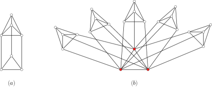
Figure 4: $(a)$ $P^{3}_{2}$; and $(b)$ $H^{3}_{2}$.

Now, we will show that $\mathrm{pe}(H^{k}_{\ell})=\ell$. Let $S\subseteq V(H^{k}_{\ell})$ be the base of $H^{k}_{\ell}$. Since $S$ induces a complete subgraph, there is a path, say $Q$, that contains every vertex of $S$. To find an upper bound for the eccentricity of $Q$, first, we study the eccentricity of a vertex $u$ that belongs to the tail of $P^{k}_{\ell}$. Since the head of $P^{k}_{\ell}$ is isomorphic to $K_{k+1}$, there must exists a vertex $w$, in the head of $P^{k}_{\ell}$, such that $d_{P^{k}_{\ell}}(u,w)=\ell$, and thus, $\mathrm{ecc}_{P^{k}_{\ell}}(u)=\ell$. As $S$ is the tail of every induced $P^{k}_{\ell}$ in $H^{k}_{\ell}$, the previous argument implies that $\mathrm{pe}(H^{k}_{\ell})\leq\ell$. Finally, the inequality $\mathrm{pe}(H^{k}_{\ell})\geq\ell$ follows from Proposition 1.

In what follows, we analyse for which cases $H^{k}_{\ell}$ is a tight example. By Theorem 5, we must have that

$$\ell=\mathrm{pe}(H^{k}_{\ell})\leq\frac{|V(H^{k}_{\ell})|+k}{3k+2}<\ell+1.$$ (3)

On the other hand,

$$\begin{array}[]{rcl}|V(H^{k}_{\ell})|&=&(k+2)((\ell-1)k+1)+k\\ &=&(k+2)k(\ell-1)+2k+2.\\ \end{array}$$

Replacing the last equality in inequality (3), and multiplying both sides by $(3k+2)$, we obtain the following

$$(k+2)(\ell-1)k+3k+2<(\ell+1)(3k+2).$$

The last inequality is equivalent to

$$\ell k+2(\ell+k)-(\ell-1)k^{2}>0.$$ (4)

Now, we analyse inequality (4) for some values of $k$. If $k=3$, we obtain $-4\ell+15>0$ which holds for $\ell=1,2,3$. Similarly, if $k=4$, we have that $-10\ell+24>0$ which holds for $\ell=1,2$. Finally, for $k\geq 5$, inequality (4) only holds for $\ell=1$. Therefore, for $k\geq 3$, there exists a graph $G$ that attains the bound given in Theorem 5 in the following cases: $k=3$ and $\ell=1,2,3$, and $k=4$ and $\ell=1,2$, where $\ell=\mathrm{pe}(G)$. We observe that $\mathrm{pe}(H^{k}_{\ell})$ is equal to the diameter of $P^{k}_{\ell}$. Thus, it is natural to try improving the previous construction by considering a $k$-connected graph with larger diameter. Unfortunately, as noted by Caccetta & Smyth [5] (see Theorem 1), the graph $P^{k}_{\ell}$ has the largest diameter among the $k$-connected graphs with the same number of vertices.

We conclude this section observing that, if we are interested in dominating paths, that is, a path in which every vertex in the graph is at distance at most one, then Theorem 5 give us the following corollary.

Corollary 5

If $G$ is a $k$-connected graph with $k>\frac{n-4}{5}$ then $G$ has a dominating path.

Faudree et. al. [11] showed that for a $k$-connected graph $G$, if $\delta(G)>\frac{n-2}{k+2}$ then $G$ has a dominating path. As $\delta(G)\geq k$ for $k$-connected graphs, this implies that for any $k>\sqrt{n-1}-1$, any $k$-connected graph has a dominating path. Thus, Corollary 5 improves Faudree’s result for $n\leq 21$. Note that Corollary 5 gave us a result for any $k$-connected graph, independent of its minimum degree.

4 Longest paths as central paths

In the previous section, we showed upper bounds for $\mathrm{pe}(G)$ based on the eccentricity of a longest path of a graph $G$. Since a longest path maximizes the number of vertices in it, intuitively it seems a good approximation for a central path of $G$. Moreover, in graphs that contain a Hamiltonian path, longest paths and central paths coincide. This led us to study the relationship between a longest path and a central path on a graph. In particular, we are interested in investigating which structural properties ensure the following.

Property 1

Every longest path is a central path of the graph.

In what follows, we tackle this question for different classes of graphs.

4.1 Trees and planar graphs

First, we consider the case in which the input graph is a tree. In this case, every longest path contains the center(s) of a tree [7]. Cockayne et. al. [8] showed an analogous result for the case of minimum-length central paths.

Theorem 6 (Cockayne et. al., 1981)

Let $P^{*}$ be a central path of minimum length in a tree $T$. Then $P^{*}$ contains the center(s) of $T$. Moreover, $P^{*}$ is unique.

Let $P$ be a longest path of $T$. Next, we show that $P$ contains $P^{*}$.

Theorem 7

Let $T$ be a tree. Let $P$ be a longest path of $T$. If $P^{*}$ is a central path of minimum length, then $V(P^{*})\subseteq V(P)$.

Proof 12

Since $P$ and $P^{*}$ contain the center(s) of the tree, we have that

$$X:=V(P)\cap V(P^{*})\neq\emptyset.$$

Furthermore, since $T$ is a tree, the set $X$ induces a subpath of $P$ and $P^{*}$, say $X=\langle x_{1},x_{2},\ldots,x_{k}\rangle$. Suppose by contradiction that $V(P^{*})\nsubseteq V(P)$. Then, there exists an extreme of $P^{*}$, say $a$, that is not in $P$. Let $u$ be an extreme of $P$ that is nearest to $a$. Without loss of generality, suppose that $u$ is the closest extreme to $x_{1}$.

By the minimality of $P^{*}$, there exists a vertex $a^{\prime}\notin V(P^{*})$ such that

$$\begin{array}[]{rcl}d_{T}(a,a^{\prime})&=&\mathrm{ecc}(P^{*}),\\ d_{T}(b,a^{\prime})&>&\mathrm{ecc}(P^{*}),\text{ for }b\in V(P^{*})\setminus\{a\}.\end{array}$$ (5)

Moreover, observe that $a^{\prime}\notin V(P)$, otherwise we have

$$\min\{d_{T}(x_{1},a^{\prime}),d_{T}(x_{k},a^{\prime})\}<d_{T}(a,a^{\prime}),$$

which contradicts $(\ref{eq:minimal})$. Thus, $a^{\prime}\in V(T)\setminus(V(P^{*})\cup V(P))$. Moreover, the path linking $a$ to $a^{\prime}$, in $T$, does not contain any vertex of $P$ or $P^{*}$ (except $a$). Otherwise, there exists a vertex, in $P^{*}$, that is closer to $a^{\prime}$ than $a$. Let $Q$ be the path between the vertices $x_{1}$ and $a^{\prime}$. Also, let $R$ be the path obtained from $P$ by replacing the path from $u$ to $x_{1}$ by $Q$. Since $|R|\leq|P|$, we have that

$$d_{T}(u,x_{1})\geq d_{T}(a^{\prime},x_{1})>d_{T}(a,a^{\prime})=\mathrm{ecc}(P^{*})\geq d_{T}(u,x_{1}),$$

where the second inequality follows from $(\ref{eq:minimal})$. Therefore, we have a contradiction.

The previous result implies the following.

Corollary 6

If $G$ is a tree, a longest path is a central path of $G$.

A natural direction is to extend the previous result for classes of graphs that contain trees. A minimal such superclass is cacti. That is, the connected graphs where any two cycles have at most one vertex in common. As shown by Figure 5 $(a)$, in this class, there are graphs such that a longest path is not a central path. In this figure, a longest path is composed of the vertices in the two cycles, which has eccentricity three, whereas the path eccentricity of the graph is two.

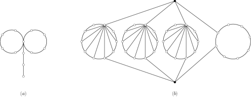
Figure 5: Two graphs that do not satisfy Property 1: $(a)$ a cactus; and $(b)$ a $2$-connected planar graph.

Now, if we impose that a cactus is $2$-connected, then Property 1 holds, as these graphs are precisely cycles. Moreover, this additional constraint also ensures this property for a broader class of graphs. We say that a graph is outerplanar if it can be embedded in the plane such that all its vertices belong to the outer face (and thus every cactus is outerplanar). Sysło [20] showed that $2$-connected outerplanar graphs are Hamiltonian, and therefore satisfy Property 1.

On the contrary, when we consider $2$-connected planar graphs, Property 1 does not hold, as shown by Figure 5 $(b)$. In this figure, if we remove the black vertices, the resulting graph has four components: three having ten vertices and one having eight vertices. Clearly, every longest path is composed of the black vertices, and the vertices on the components with ten vertices. This implies that every longest path has eccentricity three. On the other hand, the path eccentricity of the graph is two. We can obtain such a path, by considering a path that contains the two black vertices, and the vertices that belong to the cycle of eight vertices. Tutte [21] showed that $4$-connected planar graphs are Hamiltonian, thus every longest path is central. Therefore, by imposing a higher vertex-connectivity, we can ensure Property 1 on planar graphs. We observe that, it is still open whether this property is also satisfied by $3$-connected planar graphs.

4.2 Classes with bounded path eccentricity

In this section, we study Property 1 on classes of graphs that have bounded path eccentricity. A graph is AT-free if for every triple of vertices, there exists a pair of vertices in that triple, such that every path between them contains a neighbor of the other vertex of the triple. Corneil et. al. [9] showed that every AT-free graph admits a dominating path. A natural question is whether admitting a dominating path (or having bounded path eccentricity) implies that a longest path is also central. In what follows, we show a counterexample to this question.

A graph $G$ is called an interval graph if there exists a set of intervals (representing the vertices of the graph), in $\mathbb{R}$, such that two vertices are adjacent if and only if its corresponding intervals intersect. Let $k\geq 3$ be an integer. Let $G$ be the interval graph of the following set of intervals.

$$\begin{array}[]{rcll}A_{i}&=&[1,2^{k-i}],&\text{for }i=1,\ldots,k,\\ B_{i}&=&[2^{k-1}+1,2^{k-1}+2^{k-i}],&\text{for }i=1,\ldots,k,\\ C_{i}&=&[2^{k}+i,2^{k}+i+1],&\text{for }i=1,\ldots,k-1,\\ D&=&[1,2^{k}+1].\end{array}$$

In Figure 6, we show an example of $G$ for $k=3$.

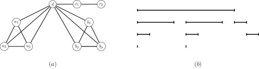
Figure 6: $(a)$ an interval graph $G$; and $(b)$ its interval representation.

As $G$ is an interval graph and, thus an AT-free graph [16], we have that $\mathrm{pe}(G)\leq 1$. Let $a_{i}$ be the vertex representing interval $A_{i}$, for $i=1,\ldots,k$. In a similar way, we define the vertices $b_{i}$, $c_{i}$ and $d$. Observe that $P=\langle a_{k},a_{k-1},\ldots,a_{1},d,b_{1},\ldots,b_{k}\rangle$ is a longest path in $G$, and $\mathrm{ecc}_{G}(P)=k-1$. Indeed, every longest path of $G$ has eccentricity $k-1$. On the other hand, the path $Q=\langle a_{k},\ldots,a_{1},d,c_{1},\ldots,c_{k-1}\rangle$ has eccentricity one. Furthermore, $Q$ is a central path of $G$.

We observe that, in the previous example, the interval representation of $G$ contains intervals that are properly included in other intervals. We say that a graph $G$ is a proper interval graph if it admits an interval representation where no interval is properly contained in another interval. Bertossi [2] showed that every connected proper interval graph has a Hamiltonian path (see Lemma 2). Therefore, we have the following.

Corollary 7

If $G$ is a proper interval graph, a longest path is a central path of $G$.

Now, we focus on bipartite graphs that have bounded path eccentricity. In Section 2, we showed that convex graphs have path eccentricity at most two. As shown by Figure 7, convex graphs do not satisfy Property 1. Let $G=(X\cup Y,E)$ denote the graph in this figure. The set $X$ is depicted by the white vertices. The labels on these vertices represent a convex ordering of $X$. Observe that, if we remove the vertex $s$, the resulting graph has three components, two of size eight and one of size four. Thus, every longest path of $G$ is composed of $s$ and the vertices in the bigger components. Then, the eccentricity of any longest path, in $G$, is four. On the other hand, $\mathrm{pe}(G)\leq 2$ by Corollary 1.

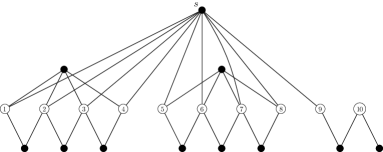
Figure 7: A convex graph that does not satisfy Property 1.

To conclude this section, we consider bipartite permutation graphs, a subclass of convex graphs. By Theorem 2, we have that $\mathrm{pe}(G)\leq 1$ for every bipartite permutation graph $G$. Now, suppose that $G$ does not admit a Hamiltonian path. The following result from Cerioli et. al. [6] implies that $\mathrm{ecc}_{G}(P)=1$, for every longest path $P$.

Lemma 4 (Cerioli et. al., 2018)

Let $G$ be a bipartite permutation graph, and let $uv\in E(G)$. Every longest path contains a vertex in $\{u,v\}$.

Therefore, Property 1 holds for this class.

Corollary 8

If $G$ is a bipartite permutation graph, a longest path is a central path of $G$.

5 Open problems and concluding remarks

In this work, we studied the path eccentricity of graphs. First, we considered subclasses of perfect graphs. We showed that convex (resp. biconvex) graphs have path eccentricity at most two (resp. one). Moreover, we exhibit graphs that attain these bounds, and design polynomial-time algorithms for finding such paths. We observe that the adjacency matrix (or a submatrix of it) of a graph in these classes exhibit the consecutive ones property [13]. This property also appears in interval graphs (which have path eccentricity one). So, we believe the following question is important to understand the class of graphs that have bounded path eccentricity.

Question 1

How does the consecutive ones property (or variations of it) influence the path eccentricity of a graph?

After that, we studied the path eccentricity of $k$-connected graphs, for $k\geq 1$. We showed a tight upper bound for this class. Interestingly, a graph that attains this bound has path eccentricity one. We posed the following question: there exists a $k$-connected graph, with path eccentricity $\ell$, that attain this bound? We give an affirmative answer for the cases: $k\leq 2$ and $\ell\geq 1$; $k=3$ and $\ell=1,2,3$; $k=4$ and $\ell=1,2$; and $k\geq 5$ and $\ell=1$. It is open whether such graph exists for $k=3$ and $\ell\geq 4$; $k=4$ and $\ell\geq 3$; and $k\geq 5$ and $\ell\geq 2$. If such graphs do not exist, then the bound we obtained for $k$-connected graphs can be improved for $k\geq 3$. We consider interesting to study this question for $k=3$.

Question 2

Do there exists a better bound for $\mathrm{pe}(G)$ when $G$ is 3-connected?

To obtain the result for $k$-connected graphs, we studied the eccentricity of a longest path in a graph. It is natural to think that a path that contains the maximum number of vertices would also be a good candidate (or approximation) for a central path. For that reason, we investigated what structural properties imply that, in a graph, a longest path is also central. In what follows, we refer to this property as Property 1. We showed that Property 1 is satisfied by trees. Furthermore, we consider subclasses of planar graphs that contain trees. We observe that, under an additional connectivity constraint, Property 1 is satisfied by cactus, outerplanar and planar graphs. This observation leads to the following question. Let $f$ be a function that, given a class of graphs, returns the minimum integer $k^{*}$ such that a $k^{*}$-connected graph, in this class, satisfies Property 1. Note that, a trivial bound for this function follows from Ore’s Theorem [3] with $k^{*}=(n-1)/2$, where $n$ is the number of vertices of the graph, since a graph $G$ with $\delta(G)\geq(n-1)/2$ contains a Hamiltonian path. In particular, we exhibit tight bounds for this function on cactus and outerplanar graphs, and a constant upper bound for planar graphs.

Question 3

Investigate better upper bounds for $f$, in general, or in some classes of graphs.

References

- [1] N. Abbas and L. Stewart. Biconvex graphs: ordering and algorithms. Discrete Appl. Math., 103(1-3):1–19, 2000.
- [2] A. Bertossi. Finding Hamiltonian circuits in proper interval graphs. Inform. Process. Lett., 17(2):97–101, 1983.
- [3] J. Bondy and U. Murty. Graph theory, volume 244 of Graduate Texts in Mathematics. Springer, New York, 2008.
- [4] K. Booth and G. Lueker. Testing for the consecutive ones property, interval graphs, and graph planarity using -tree algorithms. J. Comput. System Sci., 13(3):335–379, 1976.
- [5] L. Caccetta and W. Smyth. Graphs of maximum diameter. Discrete Math., 102(2):121–141, 1992.
- [6] M. Cerioli, C. Fernandes, R. Gómez, J. Gutiérrez, and P. Lima. Transversals of longest paths. Discrete Math., 343(3):111717, 10, 2020.
- [7] G. Chartrand, L. Lesniak, and P. Zhang. Graphs & digraphs. Textbooks in Mathematics. CRC Press, Boca Raton, FL, sixth edition, 2016.
- [8] E. Cockayne, S. M. Hedetniemi, and S. T. Hedetniemi. Linear algorithms for finding the Jordan center and path center of a tree. Transp. Sci., 15(2):98–114, 1981.
- [9] D. Corneil, S. Olariu, and L. Stewart. Asteroidal triple-free graphs. SIAM J. Discrete Math., 10(3):399–430, 1997.
- [10] P. Erdős, J. Pach, R. Pollack, and Z. Tuza. Radius, diameter, and minimum degree. J. Combin. Theory Ser. B, 47(1):73–79, 1989.
- [11] R. Faudree, R. Gould, M. Jacobson, and D. West. Minimum degree and dominating paths. J. Graph Theory, 84(2):202–213, 2017.
- [12] M. Garey, D. Johnson, and R. Tarjan. The planar Hamiltonian circuit problem is NP-complete. SIAM J. Comput., 5(4):704–714, 1976.
- [13] M. Golumbic. Algorithmic graph theory and perfect graphs, volume 57 of Annals of Discrete Mathematics. Elsevier Science B.V., Amsterdam, second edition, 2004. With a foreword by Claude Berge.
- [14] J. Harant. An upper bound for the radius of a -connected graph. Discrete Math., 122(1-3):335–341, 1993.
- [15] J. Keil. Finding Hamiltonian circuits in interval graphs. Inform. Process. Lett., 20(4):201–206, 1985.
- [16] C. Lekkerkerker and J. Boland. Representation of a finite graph by a set of intervals on the real line. Fund. Math., 51:45–64, 1962/63.
- [17] H. Müller. Hamiltonian circuits in chordal bipartite graphs. Discrete Math., 156(1-3):291–298, 1996.
- [18] P. Slater. Locating central paths in a graph. Transp. Sci., 16(1):1–18, 1982.
- [19] J. Spinrad, A. Brandstädt, and L. Stewart. Bipartite permutation graphs. Discrete Appl. Math., 18(3):279–292, 1987.
- [20] M. Sysło. Characterizations of outerplanar graphs. Discrete Math., 26(1):47–53, 1979.
- [21] W. Tutte. A theorem on planar graphs. Trans. Amer. Math. Soc., 82:99–116, 1956.
- [22] R. Uehara and G. Valiente. Linear structure of bipartite permutation graphs and the longest path problem. Inform. Process. Lett., 103(2):71–77, 2007.
- [23] C. Yu and G. Chen. Efficient parallel algorithms for doubly convex-bipartite graphs. Theoret. Comput. Sci., 147(1-2):249–265, 1995.