Communication Efficient Federated Learning via Ordered ADMM in a Fully Decentralized Setting

Abstract

The challenge of communication-efficient distributed optimization has attracted attention in recent years. In this paper, a communication efficient algorithm, called ordering-based alternating direction method of multipliers (OADMM) is devised in a general fully decentralized network setting where a worker can only exchange messages with neighbors. Compared to the classical ADMM, a key feature of OADMM is that transmissions are ordered among workers at each iteration such that a worker with the most informative data broadcasts its local variable to neighbors first, and neighbors who have not transmitted yet can update their local variables based on that received transmission. In OADMM, we prohibit workers from transmitting if their current local variables are not sufficiently different from their previously transmitted value. A variant of OADMM, called SOADMM, is proposed where transmissions are ordered but transmissions are never stopped for each node at each iteration. Numerical results demonstrate that given a targeted accuracy, OADMM can significantly reduce the number of communications compared to existing algorithms including ADMM. We also show numerically that SOADMM can accelerate convergence, resulting in communication savings compared to the classical ADMM.

I Introduction

In recent years, distributed optimization/learning algorithms have created a great deal of interest, with particular emphasis on approaches that attempt to optimize a performance criterion employing available data stored at local devices. The basic idea in distributed learning is to parallelize the computing process across multiple local devices (a.k.a. workers or nodes) to solve the following distributed learning problem

$$\min_{\bm{\theta}\in\mathbb{R}^{q}}\mathcal{L}(\bm{\theta})\quad\text{ with }\quad\mathcal{L}(\bm{\theta})\buildrel\Delta\over{=}\sum_{m\in\mathcal{M}}\mathcal{L}_{m}(\bm{\theta})$$ (1)

where $\bm{\theta}\in\mathbb{R}^{q}$ is the model parameter vector, $\mathcal{L}(\bm{\theta})$ is the global objective function, and $\mathcal{L}_{m}(\bm{\theta})$ is the local function for worker $m\in\mathcal{M}=\{1,2,...,M\}$ that is often defined as $\mathcal{L}_{m}(\bm{\theta})\buildrel\Delta\over{=}\sum_{n=1}^{N_{m}}\ell(\bm{\theta};\bm{x}_{n},y_{n})$ where $\ell(\bm{\theta};\bm{x}_{n},y_{n})$ is the loss function for $n=1,2,...,N_{m}$, $\bm{x}_{n}$ is the $n$-th feature vector and $y_{n}$ is the corresponding label. One common approach to solve (1) is a worker-server architecture where the server regularly broadcasts the model parameter to all workers, the workers calculate their local gradients based on the received model parameter and send them back to the central server, and finally the server aggregates the gradients received from all workers to update the model parameter. However, this architecture may be impractical in some cases and the server becomes a potential single point of failure [1, 2].

In this paper, we consider a more general and robust distributed network architecture where each worker exchanges information with its neighbors. Each node then updates its model parameter based on the information from its neighbors. Although this fully decentralized architecture enjoys better scalability, a very large number of communications among all the nodes are typically required to solve (1). In a wireless communications setting a large number of transmissions is undesirable due to energy consumption. Thus, reducing the number of communications is highly desirable. In addition, for typical computing hardware, the latency to send data over a network connection is much larger than that for accessing data in its own main memory [3]. Thus, the communications can be a significant bottleneck that lengthens the overall time to complete an algorithm. The goal of this paper is to develop a class of communication-efficient distributed learning algorithms to accurately solve (1) while reducing the communications in a fully decentralized architecture setting.

A straightforward method to enhance communication efficiency is to accelerate convergence, which also tends to reduce communications. Some researchers have proposed one-shot parameter averaging methods in [4, 5, 6] to find the optimal minimizer using only one iteration, which might not be stable in some cases [7]. Some popular primal-dual methods [3, 8, 9, 10] are also shown to be efficient in federated learning where the primal solution is obtained by efficiently solving the dual problem. Another alternative uses alternating direction method of multipliers (ADMM) algorithms where the workers alternate between computing the dual variables in a distributed way, and solving augmented Lagrangian problems based on their own data [7, 11, 12, 13, 14, 15, 16, 17, 18]. These algorithms are very effective, and so it is of interest to devise versions of ADMM that require fewer transmissions to achieve a given accuracy.

Censoring has been shown to be an effective method to improve efficiency, where workers only transmit highly informative data and thereby reduce the number of transmissions [19]. In [20] ADMM with censoring (censoring-ADMM) was proposed, that restricts each worker from transmitting its local message to neighbors if it is not sufficiently different from the previously transmitted one, and neighbors can use the past received value from that worker to approximate the current one. The sufficiency of the difference needed for transmission is adaptively determinted using a predefined censoring function. However, there are some aspects of ADMM and transmission reduction that have not yet been explored. For example, in censoring-ADMM, each worker independently decides whether to transmit or not without interacting with other workers. Our proposed algorithm gains substantial performance enhancement by exploiting how transmissions can be arranged in time and processed such that workers can collaboratively decide what is the most informative data to transmit to their neighbors.

Our proposed algorithms employ ordering such that at each iteration nodes with more informative data transmit their messages sooner [21]. To the best of our knowledge, ordered transmissions have not been applied to federated learning in a completely distributed setting. Some extensions to the work in [21] have been developed, including the application of ordering to quickest change detection in sensor networks [22], nearest-neighbor learning [23], and ordered gradient descent (GD) in a worker-server architecture setting [24].

In this paper we develop ordered ADMM (OADMM), with the goal of finding the model parameter $\bm{\theta}$ that minimizes (1) while reducing the communications among the nodes with respect to those required for ADMM for a given network topology. Similar to censoring-ADMM, a node is allowed to transmit its local variable to its neighbors only if its current local variable is significantly different from its previously transmitted one. The key novelty of OADMM is that for each iteration (i) the transmission-ordering strategy is employed, and (ii) every node will update its local estimate using the information received prior to its own transmission time. (The transmission time for each node is fixed at the beginning of each iteration, and the mid-iteration update in (ii) does not alter the ordering.) Thus, the most informative data is used by all neighbors who have not yet transmitted, and numerical results show that ordering and processing in this way yields significant communication savings. A cutoff time threshold is employed such that for each iteration, only a subset of the nodes (the most informative nodes based on ordering) will transmit. Furthermore, when we allow all nodes to transmit at each iteration (by not employing the cutoff time threshold), OADMM reduces to a variant of the classical ADMM, called SOADMM, which is also shown to have a better convergence behavior than ADMM thanks to ordering.

II Classical ADMM

Before introducing OADMM, we first establish the model and briefly review ADMM in the decentralized setting. The network is characterized by an underlying undirected graph $\mathcal{G}=\{\mathcal{M},\mathcal{E}\}$, where $\mathcal{M}=\{1,2,...,M\}$ is a set of nodes and $\mathcal{E}$ denotes the set of undirected edges of the graph. Note that in this paper, the terms “worker” and “node” are used interchangeably. Node $m$ and node $m^{\prime}$ are called neighbors if the edge $(m,m^{\prime})\in\mathcal{E}$. We denote the set of neighbors of node $m$ as $\mathcal{N}_{m}$ with $d_{m}=|\mathcal{N}_{m}|$.

To solve (1) with classical ADMM, at each iteration $k$ each node $m$ broadcasts its local solution ${\bm{\theta}}_{m}^{k}$ to its neighbors and then updates its local estimate using

$${\bm{\theta}}_{m}^{k}=\arg\min_{{\bm{\theta}}_{m}}\mathcal{L}_{m}\left({\bm{\theta}}_{m}\right)$$

$$\quad+\left\langle{\bm{\theta}}_{m},\lambda_{m}^{k-1}-\alpha\sum_{m^{\prime}\in\mathcal{N}_{m}}\left({\bm{\theta}}_{m}^{k-1}+{\bm{\theta}}_{m^{\prime}}^{k-1}\right)\right\rangle+\alpha d_{m}\left\|{\bm{\theta}}_{m}\right\|^{2}.$$ (2)

The local dual variable $\lambda_{m}^{k}$ is then computed using

$$\lambda_{m}^{k}=\lambda_{m}^{k-1}+\alpha\sum_{m^{\prime}\in\mathcal{N}_{m}}\left({\bm{\theta}}_{m}^{k}-{\bm{\theta}}_{m^{\prime}}^{k}\right).$$ (3)

Each ADMM iteration typically requires $\sum_{m=1}^{M}d_{m}$ communications, and this can be significantly reduced using OADMM as described next.

III Ordering-based ADMM

In this section, we consider applying ordering to ADMM in a general network architecture setting where each worker communicates with a subset of the other workers in the network.

Like classical ADMM, OADMM is synchronous such that all nodes start each iteration at the same time. Additionally, we denote $\Delta_{k}$ as the cutoff time threshold of iteration $k$ and denote $t_{k}$ as the starting time of iteration $k$. It follows that $t_{k+1}=t_{k}+\Delta_{k}$ for $k=1,2,...,K$ where $K$ is the total number of iterations. At iteration $k$ of OADMM, node $m$ not only computes the primal variable ${\bm{\theta}}_{m}^{k}$ and the dual variable $\lambda_{m}^{k}$ but also stores its last dual variable $\lambda_{m}^{k-1}$ and its state variable $\hat{\bm{\theta}}_{m}^{k-1}$ that describes its most recent primal variable broadcast prior to iteration $k$. Similar to classical ADMM, besides these variables, the state variables $\hat{\bm{\theta}}_{m^{\prime}}^{k-1}$ for all its neighbors $m^{\prime}\in\mathcal{N}_{m}$ are also recorded at node $m$.

An important feature of OADMM is that nodes will transmit in order with most informative first. Specifically, at $t_{k}$ (beginning of iteration $k$), each node will calculate the initial primal variable ${\tilde{{\bm{\theta}}}_{m}^{k}}$ using

$${\tilde{{\bm{\theta}}}_{m}^{k}}=\arg\min_{{\bm{\theta}}_{m}}\mathcal{L}_{m}\left({\bm{\theta}}_{m}\right)$$

$$\quad+\left\langle{\bm{\theta}}_{m},\lambda_{m}^{k-1}-\alpha\sum_{m^{\prime}\in\mathcal{N}_{m}}\left(\hat{\bm{\theta}}_{m}^{k-1}+\hat{\bm{\theta}}_{m^{\prime}}^{k-1}\right)\right\rangle+\alpha d_{m}\left\|{\bm{\theta}}_{m}\right\|^{2}$$ (4)

where $\alpha$ is the step size and $d_{m}=|\mathcal{N}_{m}|$ is the number of neighbors of node $m$. Then, each node $m=1,\dots,M$ sets a timer and waits $\tau/(c_{0}+\|{\tilde{{\bm{\theta}}}_{m}^{k}}-\hat{\bm{\theta}}_{m}^{k-1}\|)$ seconds to broadcast to its neighbors. Here $\tau$ is a positive number that is set as small as the physical system will allow and $c_{0}$ is a predefined constant. The nodes with the largest $\|{\tilde{{\bm{\theta}}}_{m}^{k}}-\hat{\bm{\theta}}_{m}^{k-1}\|$ transmit first and the nodes with smaller values transmit later. If the transmit time exceeds the cutoff, then these nodes do not transmit. We denote the set of neighbors of node $m$ who have broadcasted before and after node $m$ at iteration $k$ as $\mathcal{N}_{m,k}^{\prime\prime}$ and $\mathcal{N}_{m,k}^{\prime}$, respectively. Note that $\mathcal{N}_{m}=\mathcal{N}_{m,k}^{\prime\prime}\bigcup\mathcal{N}_{m,k}^{\prime}$. Just before it transmits, node $m$ performs an update using the new information from its neighbors, given by

$${\bm{\theta}}_{m}^{k}=\arg\min_{{\bm{\theta}}_{m}}\mathcal{L}_{m}\left({\bm{\theta}}_{m}\right)$$

$$\qquad+\left\langle{\bm{\theta}}_{m},\lambda_{m}^{k-1}-\alpha\sum_{\begin{subarray}{c}m^{\prime}\in\mathcal{N}_{m,k}^{\prime}\end{subarray}}\left(\tilde{{\bm{\theta}}}_{m}^{k}+\hat{\bm{\theta}}_{m^{\prime}}^{k-1}\right)\right.$$

$$\qquad\left.-\alpha\sum_{\begin{subarray}{c}m^{\prime\prime}\in\mathcal{N}_{m,k}^{\prime\prime}\end{subarray}}\left(\tilde{{\bm{\theta}}}_{m}^{k}+{\bm{\theta}}_{m^{\prime\prime}}^{k}\right)\right\rangle+\alpha d_{m}\left\|{\bm{\theta}}_{m}\right\|^{2}.$$ (5)

Immediately after broadcasting, node $m$ will update its own state variable $\hat{\bm{\theta}}_{m}^{k}={\bm{\theta}}_{m}^{k}$. During iteration $k$, if node $m$ for all $m=1,2,...,M$ receives the primal variable ${\bm{\theta}}_{m^{\prime}}^{k}$ from its neighbor $m^{\prime}\in\mathcal{N}_{m}$, then node $m$ will locally update the information about its neighbor by setting $\hat{\bm{\theta}}_{m^{\prime}}^{k}={\bm{\theta}}_{m^{\prime}}^{k}$. If such an update does not occur, then the value of this variable at node $m$ maintains its previous value $\hat{\bm{\theta}}_{m^{\prime}}^{k}=\hat{\bm{\theta}}_{m^{\prime}}^{k-1}$. Any nodes who have not yet transmitted prior to time ($t_{k}+{\Delta_{k}}$) will not transmit during iteration $k$. At time ($t_{k}+{\Delta_{k}}$), node $m$ will compute its dual variable $\lambda_{m}^{k}$ (for $m=1,\ldots,M$) using

$$\lambda_{m}^{k}=\lambda_{m}^{k-1}+\alpha\sum_{m^{\prime}\in\mathcal{N}_{m}}\left(\hat{\bm{\theta}}_{m}^{k}-\hat{\bm{\theta}}_{m^{\prime}}^{k}\right).$$ (6)

OADMM is summarized in Algorithm 1. If all transmission propagation delays are known and timing is synchronized, one can schedule all transmissions so they arrive in the correct order. However, even with imperfect synchronization a node can put them back in order correctly as long as the node waits a short period relative to the uncertainty; see [25].

Setting the cutoff time threshold to be ${\Delta_{k}}=\tau/c_{0}$ effectively eliminates the cutoff so that every node transmits in each iteration. We call this variation SOADMM. Compared to the classical ADMM, numerical results in Section IV show that both OADMM and SOADMM can save communications for a given accuracy, and SOADMM can accelerate convergence.

Algorithm 1 OADMM.

1:Assume syn. and known transmission delays (see first new paragraph after (6) for relaxing.).

2:step size $\alpha$, constants $c_{0}>0$, $c_{1}>0$, $0<\rho<1$, and $\tau>0$.

3:{${\bm{\theta}}_{m}^{0}=0$, $\lambda_{m}^{0}=0$, $\hat{\bm{\theta}}_{m}^{0}=0$, $\forall m$}

4:for $k=1,2,...,K$ do

5:     Each node $m$ updates its initial primal variable ${\tilde{{\bm{\theta}}}_{m}^{k}}$ via (III) at the starting time $t_{k}$ of iteration $k$.

6:     Each node $m$ will determine a time $t_{m,k}=t_{k}+\tau/(c_{0}+\|{\color[rgb]{0.00,0.00,0.00}\tilde{{\bm{\theta}}}_{m}^{k}}-\hat{\bm{\theta}}_{m}^{k-1}\|)$ to broadcast.

7:     Order nodes $m_{1},...,m_{M}$ using $t_{k}\leq t_{m_{1},k}\leq t_{m_{2},k}\leq...\leq t_{m_{M},k}$.

8:     Set $i=1$ and ${\Delta_{k}}=\tau/{(c_{0}+c_{1}\rho^{k})}$.

9:     while $i\leq M$ do

10:         if $t_{m_{i},k}\leq t_{k}+{\Delta_{k}}$ then

11:              At time $t_{m_{i},k}$, node $m_{i}$ updates ${\bm{\theta}}_{m_{i}}^{k}$ via (III) .

12:              At time $t_{m_{i},k}$, node $m_{i}$ broadcasts ${\bm{\theta}}_{m_{i}}^{k}$ to all of its neighbors and updates its state variable $\hat{\bm{\theta}}_{m_{i}}^{k}={\bm{\theta}}_{m_{i}}^{k}$ immediately after broadcasting.

13:              At time $t_{m_{i},k}$, all neighbors of node $m_{i}$ update the information about node $m_{i}$ as $\hat{\bm{\theta}}_{m_{i}}^{k}={\bm{\theta}}_{m_{i}}^{k}$.

14:         else

15:              At time $t_{k}+{\Delta_{k}}$, node $m_{i}$ updates its state variable $\hat{\bm{\theta}}_{m_{i}}^{k}=\hat{\bm{\theta}}_{m_{i}}^{k-1}$.

16:              At time $t_{k}\!+\!{\Delta_{k}}$, all neighbors of node $m_{i}$ update information about node $m_{i}$ as $\hat{\bm{\theta}}_{m_{i}}^{k}\!\!=\!\hat{\bm{\theta}}_{m_{i}}^{k-1}$​.

17:         end if

18:         At time $t_{k}+{\Delta_{k}}$, node $m_{i}$ updates its local dual variable $\lambda_{m_{i}}^{k}$ via (6).

19:         Set $i=i+1$.

20:     end while

21:end for

IV Numerical Results

Consider the linear regression task studied in [20], with the local function at worker $m$ in (1) being

$$\mathcal{L}_{m}(\bm{\theta})\buildrel\Delta\over{=}\frac{1}{2}\sum_{n=1}^{{N}_{m}}\left(y_{n}-\mathbf{x}_{n}^{\top}\bm{\theta}\right)^{2}$$ (7)

where $y_{n}$ is the $n$-th label and $\mathbf{x}_{n}$ is the corresponding feature vector. Let ${\bm{\theta}}^{*}$ denote the optimal solution. Each scalar in the vector $(({\bm{\theta}}^{*})^{\top},\mathbf{x}_{1}^{\top},\ldots,\mathbf{x}_{N_{m}}^{\top})$ is chosen uniformly from the set $[0.1,0.2,...,1]$ and we obtain $y_{n}$ by using $y_{n}=\mathbf{x}_{n}^{\top}{\bm{\theta}}^{*}$. We set $M=50$ and $N_{m}=3$ for all $m=1,...,M$. We compare the performance of OADMM with classical ADMM, censoring-based ADMM [20], and SOADMM using the same setting/problem as in [20] to provide a favorable environment for censoring-based ADMM. As in [20], the network has $10\%$ of all possible edges randomly chosen to be connected. The step size $\alpha=0.4$ is used for all four algorithms. We employ the optimized stopping threshold $c_{1}\rho^{k}$ ($c_{1}=5$, $\rho=0.87$) in censoring-based ADMM [20]. We allow workers to transmit at iteration $k$ in OADMM if $\|\tilde{{\bm{\theta}}}_{m}^{k}-\hat{\bm{\theta}}_{m}^{k-1}\|\geq c_{1}\rho^{k}$ and let all workers transmit in SOADMM.

Let ${\bm{\theta}}_{m}^{0}$ denote the initial value of ${\bm{\theta}}_{m}^{k}$. Define the accuracy at iteration $k$ as ${\it A}_{k}=(\sum_{m=1}^{M}\|{\bm{\theta}}_{m}^{k}-{\bm{\theta}}^{*}\|^{2})/(\sum_{m=1}^{M}\|{\bm{\theta}}_{m}^{0}-{\bm{\theta}}^{*}\|^{2})$. The accuracy ${\it A}_{k}$ is plotted versus the number of iterations $k$ in Fig. 1(a). By counting the total number of communication transmissions during each iteration $k$, the accuracy is plotted in Fig. 1(b) versus the total number of transmissions by all the nodes up to the $k$-th iteration. Fig. 1 illustrates that OADMM is able to significantly reduce the total number of transmissions when compared to ADMM, censoring-based ADMM [20], and SOADMM. Given a target accuracy of $10^{-8}$, OADMM can save about $70\%$ of the total transmissions compared to classical ADMM. Comparing Fig. 1(a) and 1(b), to reach the same accuracy, SOADMM requires fewer iterations whereas OADMM requires fewer total transmissions.

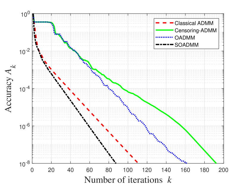
(a) Accuracy versus number of iterations

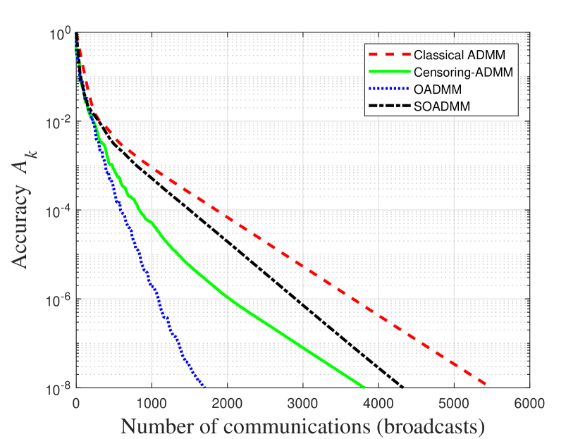
(b) Accuracy versus number of transmissions

Figure 1: Accuracy versus (a) the number of iterations, and (b) the total number of communications, for the linear regression example with a random network topology.

In Fig. 2, we plot the number of communications needed to achieve accuracy $10^{-8}$ for OADMM and ADMM versus the network density. Here, density is defined as the average number of neighbors connected, divided by the network size $M$. In this example we fix $M=200$, and all other parameters are set to be the same as the previous example. Fig. 2 shows that OADMM achieves the same accuracy as ADMM with many fewer total transmissions.

ADMM requires every node to transmit at each iteration, so for ADMM the total number of transmissions scales directly with the number of iterations needed to achieve the desired accuracy. Note that when ADMM is applied to linear regression, it is possible to optimize the stepsize for different network densities [16]. Here we continue to use the stepsize from Fig. 1 which was suggested in [20]. Fig. 2 shows that, for this range of densities, OADMM is less sensitive to the changing network density and generally saves more than half the total number of transmissions.

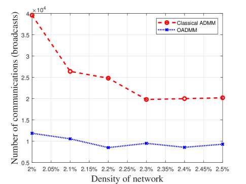
Figure 2: Total number of transmissions to achieve $10^{-8}$ accuracy versus the network density (percentage of all possible edges) for linear regression with a random network topology ($M=200$).

V CONCLUSIONS

We devised OADMM, a communication-efficient version of ADMM, to accurately solve fully distributed learning tasks. OADMM is able to significantly reduce the number of communications between workers compared to ADMM, saving energy and potentially reducing the time to solution. Transmissions are ordered at each iteration such that a worker with more informative data broadcasts its local variable sooner, and its neighbors take advantage of this received information to update their local variables before they broadcast during the current iteration. Thus, compared with ADMM, OADMM requires that some nodes perform an additional computation within each iteration. Similar to censoring, a worker is not allowed to broadcast if its current local variable is not sufficiently different from its previously transmitted one, and its neighbors use the last received value from that worker to approximate the current one.

OADMM employs a cutoff time, while a variant called SOADMM allows all workers to transmit at each iteration. Compared with ADMM, SOADMM accelerates convergence (requires fewer total iterations), whereas OADMM may require more iterations but use fewer total transmissions. Numerical results show that both OADMM and SOADMM require many fewer total transmissions than ADMM to achieve the same accuracy. It is of interest in future work to show theoretical convergence properties of OADMM and SOADMM. It may also be possible to combine OADMM with quantization and/or sparsification techniques to further reduce the communications load in bits. Robust operation is also of practical interest, to relax the network timing requirements. Asynchronous operation is also of great interest.

References

- [1] R. Xin, S. Kar, and U. A. Khan, “Decentralized stochastic optimization and machine learning: A unified variance-reduction framework for robust performance and fast convergence,” IEEE Signal Processing Magazine, vol. 37, no. 3, pp. 102–113, 2020.
- [2] A. G. Roy, S. Siddiqui, S. Pölsterl, N. Navab, and C. Wachinger, “Braintorrent: A peer-to-peer environment for decentralized federated learning,” arXiv preprint arXiv:1905.06731, 2019.
- [3] V. Smith, S. Forte, C. Ma, M. Takáč, M. I. Jordan, and M. Jaggi, “Cocoa: A general framework for communication-efficient distributed optimization,” The Journal of Machine Learning Research, vol. 18, no. 1, pp. 8590–8638, 2017.
- [4] Y. Zhang, J. C. Duchi, and M. J. Wainwright, “Communication-efficient algorithms for statistical optimization,” The Journal of Machine Learning Research, vol. 14, no. 1, pp. 3321–3363, 2013.
- [5] R. Mcdonald, M. Mohri, N. Silberman, D. Walker, and G. S. Mann, “Efficient large-scale distributed training of conditional maximum entropy models,” in Advances in neural information processing systems, 2009, pp. 1231–1239.
- [6] H. B. McMahan, E. Moore, D. Ramage, and B. A. y Arcas, “Federated learning of deep networks using model averaging. corr abs/1602.05629 (2016),” arXiv preprint arXiv:1602.05629, 2016.
- [7] O. Shamir, N. Srebro, and T. Zhang, “Communication-efficient distributed optimization using an approximate newton-type method,” in International conference on machine learning, 2014, pp. 1000–1008.
- [8] J. C. Duchi, A. Agarwal, and M. J. Wainwright, “Dual averaging for distributed optimization: Convergence analysis and network scaling,” IEEE Transactions on Automatic control, vol. 57, no. 3, pp. 592–606, 2011.
- [9] K. Scaman, F. Bach, S. Bubeck, L. Massoulié, and Y. T. Lee, “Optimal algorithms for non-smooth distributed optimization in networks,” in Advances in Neural Information Processing Systems, 2018, pp. 2740–2749.
- [10] L. He, A. Bian, and M. Jaggi, “Cola: Decentralized linear learning,” in Advances in Neural Information Processing Systems, 2018, pp. 4536–4546.
- [11] S. Boyd, N. Parikh, E. Chu, B. Peleato, J. Eckstein et al., “Distributed optimization and statistical learning via the alternating direction method of multipliers,” Foundations and Trends® in Machine learning, vol. 3, no. 1, pp. 1–122, 2011.
- [12] M. Hong and Z.-Q. Luo, “On the linear convergence of the alternating direction method of multipliers,” Mathematical Programming, vol. 162, no. 1-2, pp. 165–199, 2017.
- [13] W. Deng and W. Yin, “On the global and linear convergence of the generalized alternating direction method of multipliers,” Journal of Scientific Computing, vol. 66, no. 3, pp. 889–916, 2016.
- [14] R. Zhang and J. Kwok, “Asynchronous distributed admm for consensus optimization,” in International conference on machine learning, 2014, pp. 1701–1709.
- [15] A. Makhdoumi and A. Ozdaglar, “Convergence rate of distributed admm over networks,” IEEE Transactions on Automatic Control, vol. 62, no. 10, pp. 5082–5095, 2017.
- [16] W. Shi, Q. Ling, K. Yuan, G. Wu, and W. Yin, “On the linear convergence of the admm in decentralized consensus optimization,” IEEE Transactions on Signal Processing, vol. 62, no. 7, pp. 1750–1761, 2014.
- [17] W. Deng, M.-J. Lai, Z. Peng, and W. Yin, “Parallel multi-block admm with o (1/k) convergence,” Journal of Scientific Computing, vol. 71, no. 2, pp. 712–736, 2017.
- [18] Y. Wang, W. Yin, and J. Zeng, “Global convergence of admm in nonconvex nonsmooth optimization,” Journal of Scientific Computing, vol. 78, no. 1, pp. 29–63, 2019.
- [19] C. Rago, P. Willett, and Y. Bar-Shalom, “Censoring sensors: A low-communication-rate scheme for distributed detection,” IEEE Transactions on Aerospace and Electronic Systems, vol. 32, no. 2, pp. 554–568, 1996.
- [20] Y. Liu, W. Xu, G. Wu, Z. Tian, and Q. Ling, “Communication-censored admm for decentralized consensus optimization,” IEEE Transactions on Signal Processing, vol. 67, no. 10, pp. 2565–2579, 2019.
- [21] R. S. Blum and B. M. Sadler, “Energy efficient signal detection in sensor networks using ordered transmissions,” IEEE Transactions on Signal Processing, vol. 56, no. 7, pp. 3229–3235, 2008.
- [22] Y. Chen, R. S. Blum, and B. M. Sadler, “Ordering for communication-efficient quickest change detection in a decomposable graphical model,” IEEE Transactions on Signal Processing, 2021.
- [23] S. Marano, V. Matta, and P. Willett, “Nearest-neighbor distributed learning over communication channels,” IEEE Trans. Signal Process, 2013.
- [24] Y. Chen, B. M. Sadler, and R. S. Blum, “Ordered gradient approach for communication-efficient distributed learning,” in 2020 IEEE 21st International Workshop on Signal Processing Advances in Wireless Communications (SPAWC). IEEE, 2020, pp. 1–5.
- [25] R. S. Blum, “Ordering for estimation and optimization in energy efficient sensor networks,” IEEE Transactions on Signal Processing, vol. 59, no. 6, pp. 2847–2856, 2011.