Exploring the Dynamics of
the Circumcenter Map

Abstract.

Using experimental techniques, we study properties of the “circumcenter map”, which, upon $n$ iterations sends an $n$-gon to a scaled and rotated copy of itself. We also explore the topology of area-expanding and area-contracting regions induced by this map.

1. Introduction

Using simulation and visualization techniques, we explore interesting plane curves implied by a certain map applied to a generic polygon. For a preview of the graphical results, see Figures 13 and 14. Let us first define this map, called here the “circumcenter map”. Referring to Figure 1:

Definition 1 (Circumcenter Map).

Given a point $M$ and a polygon $\mathcal{P}$ with vertices $P_{1},\ldots,P_{n}$, the circumcenter map $\mathcal{C}_{M}(\mathcal{P})$ yields a new polygon $\mathcal{P}^{\prime}$ whose vertices are the circumcenters of $MP_{1}P_{2}$, $MP_{2}P_{3}$, …, $MP_{n}P_{1}$, respectively.

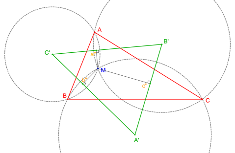
Figure 1. Given a point $M$, the circumcenter map sends a triangle $T=ABC$ to $T^{\prime}=A^{\prime}B^{\prime}C^{\prime}$ with vertices at the circumcenters of $MBC$, $MCA$, $MAB$, respectively. Also shown are the vertices $a^{\prime\prime},b^{\prime\prime},c^{\prime\prime}$ of the $M$-pedal of $T^{\prime}$ which is a half-sized version of $T$.

We review classical results that underpin the phenomena studied herein, namely:

1. $\mathcal{C}_{M}(\mathcal{P})$ yield the (half-sized) $M$-antipedal polygon, see Figure 2;

2. as a consequence of a result proved in [9], $n$ consecutive applications of this map, i.e., $\mathcal{C}_{M}^{n}(\mathcal{P})$ yields a new polygon which is the image of $\mathcal{P}$ under a rigid rotation about $M$ by $\alpha$, and a homothety (uniform scaling) with ratio $s$, see Figure 3;

3. subsequent $n$ applications of the map result in a transformation with identical parameters $\alpha$ and $s$.

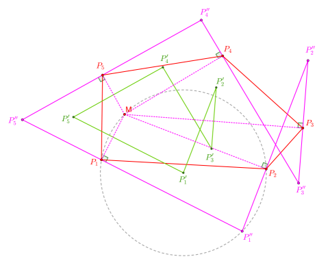
Figure 2. If $\mathcal{P}=\{P_{i}\}$ is a 5-gon (red), $\mathcal{C}_{M}(\mathcal{P})$ is another 5-gon (green) which is a half-sized version of the $M$-antipedal of $\mathcal{P}$ (magenta). Also shown is the construction for $P_{1}^{\prime}$ which is the center of circle $MP_{i}P_{i+1}$ (dashed gray).

Given a starting polygon $\mathcal{P}$, we will study the locus of $M$ such that after $n$ applications of the map the resulting polygon has the same area ($s=1$) and/or angle ($\alpha=0$) as the original one. Experiments reveal an interesting structure of such loci, and beautiful symmetries when $\mathcal{P}$ is regular, see Figure 4.

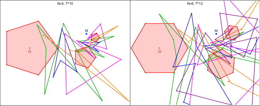
Figure 3. Left: 10 applications of the circumcenter map on a regular pentagon (left), showing 5-periodicity. Right: 12 applications starting from a regular hexagon. Note intermediate shapes are arbirtrary, see Figure 7.

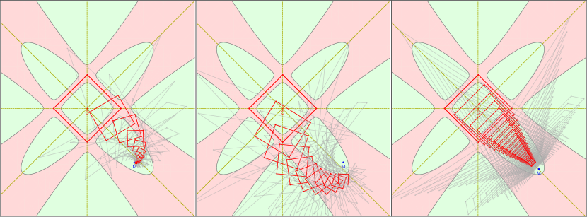
Figure 4. Iterations of the circumcenter map, starting from a square ($n=4$, red), with $M$ at an area-contracting region (green), but in locations which induce negative (left), positive (middle), or zero rotation (right) on the sequence. Intermediate iterates are shown gray, and can be of diverse shapes. Every four iterations produces a new polygon (red) which is a rotated, scaled version with respect to the original. The locus of $M$ such that $s=1$ (neutral scaling) is the boundary between the red and green regions; its shape depends on the original polygon.

Main results

The claims below were initially evidenced by simulation. Most are proved with a computer algebra system (CAS) and their proofs will be omitted.

1. We explicitly derive the locus of $M$ such that $s=1$, when $\mathcal{P}$ is an equilateral triangle (resp. a square): it is a 6-degree (resp. 8-degree) polynomial on the coordinates of $M$.

2. If $\mathcal{P}$ is a regular $n$-gon, the locus of $M$ such that $\alpha=0$ is the union of $n$ lines through the centroid of $\mathcal{P}$, rotated about each other by $\pi/n$.

3. In all cases there is a discrete set of locations such that both $s=1$ and $\alpha=0$. We study the map with $\mathcal{P}$ an equilateral triangle, showing that if $M$ is on any one of these locations the map is 3-periodic. If $M$ is at the centroid of the equilateral, the map is 2-periodic.

4. Based on compactified visualizations of the $s=1$ boundary, we conjecture that for all $n$: (i) there is only one connected region such that $s>1$, and (ii) if $n$ is odd (resp. even), the number of connected regions such that $s<1$ is given by $1+n(n+1)/2$ (resp. $1+n^{2}/2$), i.e., in both cases it is of $O(n^{2})$.

5. We informally investigate topological changes in the $s=1$ locus with respect to affine stretching of the initial polygon.

Background

In [10], properties of the “central” sub-triangle defined by a four-fold subdivision of a reference triangle (using cevians) are studied. A map based on the 2nd isodynamic point of a polygon’s subtriangles is described in [7].

Article Organization

In Section 2 we review classical results that show that $n$ applications of the circumcenter map are a similarity transform with parameters $s$ and $\alpha$ which only depend on $M$. In Section 3 we describe properties of the map for the initial polygon a triangle or a square. In Section 4 we extend the analysis to regular polygons of any number of sides. Conclusions and suggestions for further exploration appear in Section 5. To facilitate reproducibility, explicit expressions for the circumcenter map appear in Appendix A.

2. Review: Stewart’s Result

Referring to Figure 5, recall that (i) the $M$-pedal polygon of a polygon $\mathcal{P}$ has vertices at the intersections of perpendiculars dropped from $M$ onto the sides of $\mathcal{P}$; (ii) the $M$-antipedal polygon of $\mathcal{P}$ is such that $\mathcal{P}$ is its $M$-pedal. Finally, (iii) the $M$-reflection polygon of $\mathcal{P}$ has vertices at the reflections of $M$ about the sidelines of $\mathcal{P}$. Clearly:

Remark 1.

the $M$-reflection polygon of $\mathcal{P}$ is the twice-sized $M$-pedal polygon of $\mathcal{P}$, with $M$ as the homothety center.

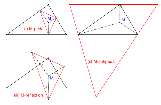
Figure 5. Constructions of pedal, antipedal, and reflection polygons, for the case of a triangle.

Let $\mathcal{P}^{\prime}=\mathcal{C}_{M}(\mathcal{P})$ be the polygon obtained under the circumcenter map of Definition 1. Let $P_{i}^{\prime},i=1\ldots n$ denote its vertices.

Lemma 1.

The polygon $\mathcal{C}_{M}^{-1}(\mathcal{P})$ is the $M$-reflection polygon $\mathcal{P}$.

Proof.

Referring to Figure 1, $P_{i}^{\prime}$ (resp. $P^{\prime}_{i+1}$) is the center of a circle $\mathcal{K}_{i}$ passing through $M,P_{i},P_{i+1}$ (resp. $\mathcal{K}_{i+1}$ passing through $M,P_{i+1},P_{i+2}$). We have that $\mathcal{K}_{i}\cap\mathcal{K}_{i+1}=\{M,P_{i}\}$.

The inverse circumcenter map is $\mathcal{C}_{M}^{-1}(\mathcal{P}^{\prime})=\mathcal{P}=\{P_{i}\}$. For each such pair of consecutive circles, the intersections $\{M,P_{i}\}$ are symmetric about $P^{\prime}_{i}P^{\prime}_{i+1}$. See Figure 1 for the case $n=3$. ∎

Using Remarks 1 and 1, the following property is illustrated in Figure 2:

Corollary 1.

$\mathcal{C}_{M}(\mathcal{P})$ is homothetic to the $M$-antipedal of $\mathcal{P}$, with ratio $1/2$ and homothety center $M$.

Recall a well-known result by Johnson [2, Theorem 2c]:

Result (Johnson, 1918).

If two polygons $\mathcal{F}$ and $\mathcal{F}^{\prime}$ with no parallel sides are similar, there exists a point $M$, called the self-homologous point, such that $\mathcal{F}^{\prime}$ is a rigid rotation of $\mathcal{F}$ about $M$ followed by uniform scaling about the same point.

Using a definition in [9, Construction 1]:

Definition 2 (Miquel Map).

Given a point $M$ and an angle $\theta$, let $\mathcal{M}$ denote a map that sends a polygon $\mathcal{P}=\{P_{i}\}$, to a new polygon $\mathcal{P}^{\prime}$ (known as the Miquel polygon) with each vertex $P^{\prime}_{i}$ is on the line $P_{i}P_{i+1}$, and such that $\measuredangle P_{i}P_{i}^{\prime}M=\theta$, for $i=1,\ldots,n$.

Let $\mathcal{M}^{k}$ denote $k$ successive applications of the Miquel map. The following key result was proved in [9, Theorem 2]:

Theorem (Stewart, 1940).

Let $\mathcal{P}$ be a polygon with $n$ sides. $\mathcal{M}^{n}(\mathcal{P})$ is similar to $\mathcal{P}$ with $M$ as the self-homologous point. If follows that if $\mathcal{M}^{j}(\mathcal{P})$ is similar to $\mathcal{M}^{i}(\mathcal{P})$, then $i\equiv j~{}(mod~{}n)$.

Let $\mathcal{M}_{\perp}$ denote the Miquel map when $\theta=\pi/2$. Definition 2 implies that $\mathcal{M}_{\perp}(\mathcal{P})$ is the pedal polygon of $\mathcal{P}$ with respect to $M$. Referring to Figure 6:

Corollary 2.

$\mathcal{M}_{\perp}^{n}(\mathcal{P})$ is self-homologous to $\mathcal{P}$, i.e., it is an image under a rigid rotation and a uniform scaling of $\mathcal{P}$ about $M$.

The inverse map $\mathcal{M}_{\perp}^{-1}(\mathcal{P})$ yields the $M$-antipedal polygon of $\mathcal{P}$. Referring to Corollary 1:

Remark 2.

$\mathcal{C}_{M}(\mathcal{P})$ is a half-sized homothety of $\mathcal{M}_{\perp}^{-1}(\mathcal{P})$ with respect to $M$.

Since the pedal transformation has an inverse, $\mathcal{M}_{\perp}^{-n}(\mathcal{P})$ is similar to $\mathcal{P}$. Referring to Figure 6, and noting that the scaling in Corollary 1 does not affect similarity:

Corollary 3.

$\mathcal{C}_{M}^{n}(\mathcal{P})$ is similar to $\mathcal{P}$.

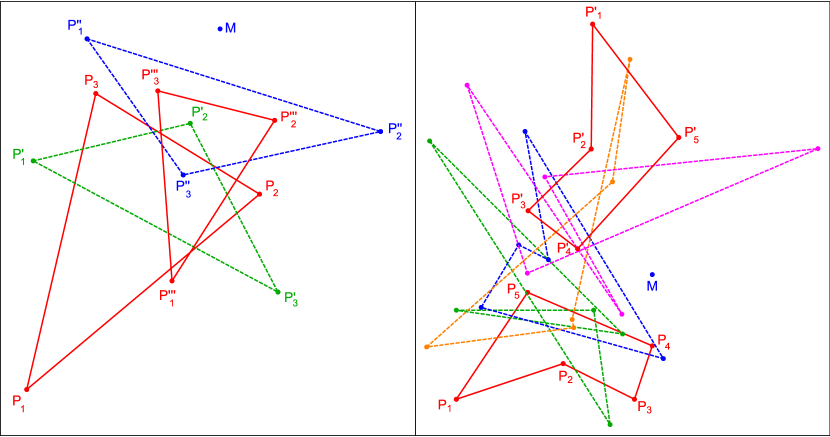
Figure 6. Left: Applying the circumcenter map with respect to $M$ to a starting triangle $P_{1}P_{2}P_{3}$ (solid red) yields the (dashed green) triangle $P_{1}^{\prime}P_{2}^{\prime}P_{3}^{\prime}$. In turn, applying the map on the latter yields the (dashed blue) triangle $P_{1}^{\prime\prime}P_{2}^{\prime\prime}P_{3}^{\prime\prime}$. Finally, a third application of the map yields $P_{i}^{\prime\prime\prime}$ (solid red), similar to the original. Right: Likewise, starting from a pentagon $P_{i}$, i=$1,\ldots,5$, $n=5$ applications of the map yields $P_{i}^{\prime}$ (dashed red), self-homologous to the original. Intermediate generations are colored dashed green, blue, orange, and magenta.

Let $\mathcal{P}^{\prime}=\mathcal{C}_{M}^{n}(\mathcal{P})$, and $\mathcal{P}^{\prime\prime}=\mathcal{C}_{M}^{2n}(\mathcal{P}^{\prime})$. Express these as $\mathcal{P}^{\prime}=\mathcal{T}(\mathcal{P})$, and $\mathcal{P}^{\prime\prime}=\mathcal{T}^{\prime}(\mathcal{P}^{\prime})$, where $\mathcal{T},\mathcal{T}^{\prime}$ are similarity transforms (that is, composition of a rotation and scaling about $M$).

Proposition 1.

$\mathcal{T}=\mathcal{T}^{\prime}$.

Proof.

Since $\mathcal{P}^{\prime}=\mathcal{T}(\mathcal{P})$, then $\mathcal{C}_{M}^{n}(\mathcal{P}^{\prime})=\mathcal{C}_{M}^{n}(\mathcal{T}(\mathcal{P}))$. By definition (see Section 1), the circumcenter map is based on the circumcenters of subtriangles of a given triangle. Since circumcenters are triangle centers (see [3]), they are equivariant over similarity transforms, therefore, $\mathcal{C}_{M}^{n}(\mathcal{T}(\mathcal{P}))=\mathcal{T}(\mathcal{C}_{M}^{n}(P))=\mathcal{T}^{2}(\mathcal{P})$, i.e., $\mathcal{C}_{M}^{n}(\mathcal{P}^{\prime})=\mathcal{T}(\mathcal{P}^{\prime})$. ∎

In Figures 3 and 7, we illustrate a statement by Stewart in [9], namely, that intermediate applications of the map produce polygons “as diverse in shape as is imaginable”.

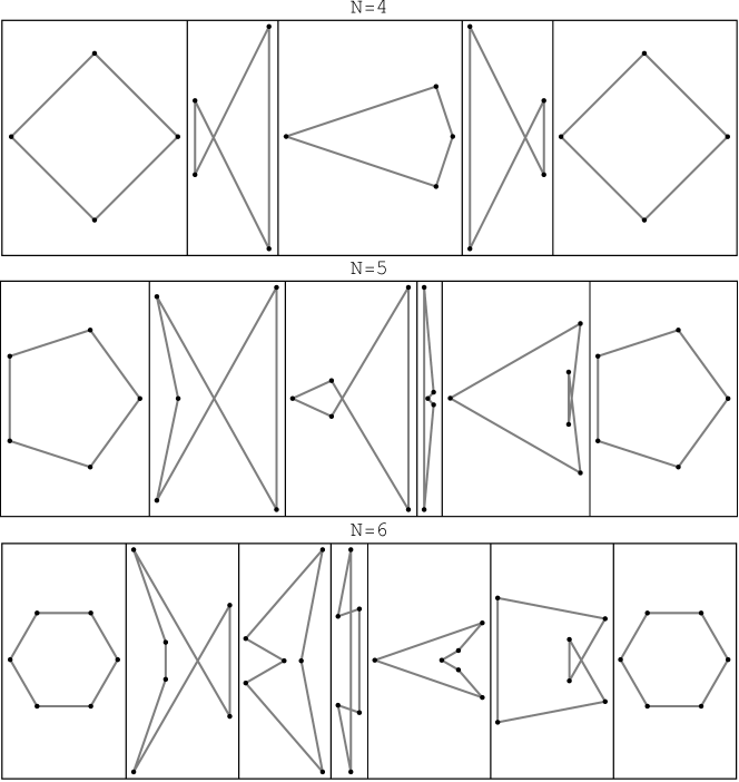
Figure 7. Intermediate shapes (with scale and rotation removed) produced by sequential applications of the circumcenter map. Top, middle, bottom strips show sequence starting from square, regular pentagon, and regular hexagon, respectively. In each case, the rightmost vertex of the starting polygon is at $(1,0)$, and $M$ (not shown) is at $(2,0)$.

3. The $n=3$ and $n=4$ cases

In this section we study the locus of $M$ such that $\mathcal{C}_{M}^{n}(\mathcal{P})$ is area-preserving ($s=1$) and/or rotation-neutral ($\alpha=0$), for the cases where $\mathcal{P}$ is an equilateral or a square.

Let $\mathcal{P}=ABC$ be a triangle, and $\mathcal{P}^{\prime}=\mathcal{C}_{M}^{3}(\mathcal{P})=A^{\prime}B^{\prime}C^{\prime}$. Let $\mathcal{A}(\mathcal{Q})$ denote the area of a polygon $\mathcal{Q}$. Via CAS, we obtain the following proposition.

Proposition 2.

The ratio of sides $A^{\prime}B^{\prime}$, $B^{\prime}C^{\prime}$ and $A^{\prime}C^{\prime}$ of $\mathcal{P}^{\prime}$ and $\mathcal{P}$ is given by:

$$\frac{|A^{\prime}B^{\prime}|}{|AB|}=\frac{|A^{\prime}C^{\prime}|}{|AC|}=\frac{|B^{\prime}C^{\prime}|}{|BC|}=\frac{{l_{a}l_{b}l_{c}m_{a}m_{b}m_{c}}}{8~{}\mathcal{A}(ABM)\mathcal{A}(BCM)\mathcal{A}(ACM)}$$

where $l_{a}=|BC|$, $l_{b}=|AC|$, $l_{c}=|AB|$, $m_{a}=|AM|$, $m_{b}=|BM|$, $m_{c}=|CM|$.

Proposition 3.

Let $\alpha$ denote the angle of rotation of $\mathcal{P}^{\prime}$ with respect to $\mathcal{P}$. Then:

$$\cos\alpha=\frac{m_{c}^{2}(m_{a}^{2}+m_{b}^{2})\mathcal{A}(ABM)+m_{b}^{2}(m_{a}^{2}+m_{c}^{2})\mathcal{A}(ACM)+m_{a}^{2}(m_{b}^{2}+m_{c}^{2})\mathcal{A}(BCM)}{l_{a}l_{b}l_{c}m_{a}m_{b}m_{c}}$$

The case of an equilateral triangle

Let $\mathcal{R}=ABC$ be the equilateral triangle with vertices $A=(1,0)$, $B=(-1,\sqrt{3})/2$, $C=(-1,-\sqrt{3})/2$. Let $\mathcal{R}^{\prime}=\mathcal{C}_{M}^{3}(\mathcal{R})$ with $M=(x_{m},y_{m})$. Let $s=\mathcal{A}(\mathcal{R}^{\prime})/\mathcal{A}(\mathcal{R})$. Via CAS, we obtain the following proposition.

Proposition 4.

If $\mathcal{P}$ is an equilateral, $s=1$ if $M=(x_{m},y_{m})$ satisfies:

$$3\,x_{m}^{6}-y_{m}^{6}-12\,x_{m}^{5}+9\,y_{m}^{4}+\left(-27\,y_{m}^{2}+9\right)x_{m}^{4}+\left(24\,y_{m}^{2}+6\right)x_{m}^{3}+$$

$$\left(33\,y_{m}^{4}+18\,y_{m}^{2}-6\right)x_{m}^{2}+\left(36\,y_{m}^{4}-18\,y_{m}^{2}\right)x_{m}-6\,y_{m}^{2}=0$$

Figures 8 and 9, illustrate sequential applications of the circumcenter map starting from an equilateral, for the cases of $M$ in an area-contracting, area-expanding, and the boundary in between them defined in Proposition 4.

Proposition 5.

If $\mathcal{P}$ is an equilateral, $\alpha=0$ when $M=(x_{m},y_{m})$ satisfies:

$$y_{m}(y_{m}^{2}-3x_{m}^{2})=0$$

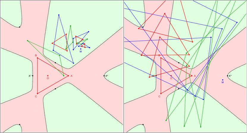
Figure 8. Left: Nine iterations of the circumcenter map starting from an equilateral triangle (solid red) centered at $O$. $M$ is placed in an area-shrinkage region (green). A new, smaller equilateral (red) is produced every 3 applications of the map. Right: with $M$ on the area-expansion region (green), the area expands upon every 3 applications of the map.

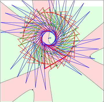
Figure 9. Starting from an equilateral (thick red) with centroid $O$, an $M$ is selected on the boundary between area-expansion (light red) and area-contraction (light green) regions. Sequential applications of the circumcenter map are shown in green, blue, and back to red. Since $M$ is on the boundary, every three applications of the map are area-preserving and result in a constant net rotation about $M$.

As shown in Figure 10, as the starting triangle is affinely distorted, the number of connected components in the $s=1$ locus changes, revealing a non-trivial relationship (not studied here).

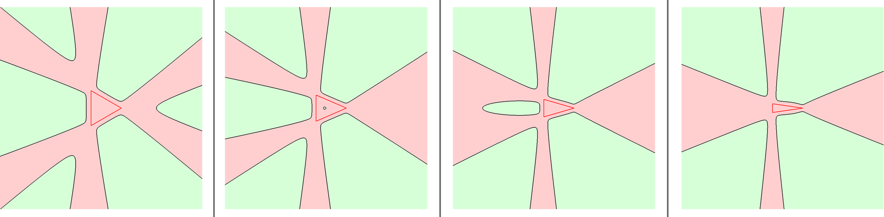
Figure 10. As the starting equilateral (red, left) is stretched horizontally, the $s=1$ boundary (under 3 applications of the circumcenter map) changes topology. See bit.ly/3Pl2tmz for interactive examples.

Referring to Figure 11:

Corollary 4.

There are six points on Proposition 4 such that $\alpha=0$. These are: $K_{1}=(1+\sqrt{3},0)$, $K_{2}=(1-\sqrt{3},0)$, and their rotations by $\pm 2\pi/3$.

Let $\mathcal{R}_{i}=A_{i}B_{i}C_{i}$ denote the image of $\mathcal{R}$ under $i$ iterations of the circumcenter map. As shown above $\mathcal{R}_{3}$ is similar to $\mathcal{R}$. Referring to Figure 11(left):

Proposition 6.

If $M=K_{1}$, then the vertices of $\mathcal{R}_{1}$ and $\mathcal{R}_{2}$ have coordinate

$$A_{1}= (1,0),\;\;\;\hskip 44.10185ptB_{1}=\left(1+\frac{\sqrt{3}}{2},\frac{3}{2}+\sqrt{3}\right),\;\;\;C_{1}=\left(1+\frac{\sqrt{3}}{2},-\frac{3}{2}-\sqrt{3}\right)$$

$$A_{2}= \left(-2-\sqrt{3},0\right),\;\;\;\;B_{2}=\left(1+\frac{\sqrt{3}}{2},\frac{3}{2}\right),\hskip 36.98866ptC_{2}=\left(1+\frac{\sqrt{3}}{2},-\frac{3}{2}\right).$$

$\mathcal{R}_{1}$ (resp. $\mathcal{R}_{2}$) has internal angles $30^{\circ},75^{\circ},75^{\circ}$ (resp. $150^{\circ},15^{\circ},15^{\circ})$.

Referring to Figure 11(right):

Proposition 7.

If $M=K_{2}$, then the vertices of $\mathcal{R}_{1}$ and $\mathcal{R}_{2}$ have coordinate

$$A_{1}= \left(1,0\right),\;\;\hskip 28.45274ptB_{1}=\left(1-\frac{\sqrt{3}}{2},-\frac{3}{2}+\sqrt{3}\right),\;\;\;C_{1}=\left(1-\frac{\sqrt{3}}{2},\frac{3}{2}-\sqrt{3}\right)$$

$$A_{2}= \left(\sqrt{3}-2,0\right),\;\;\;B_{2}=\left(1-\frac{\sqrt{3}}{2},\frac{3}{2}\right),\;\;\hskip 36.98866ptC_{2}=\left(1-\frac{\sqrt{3}}{2},-\frac{3}{2}\right).$$

$\mathcal{R}_{1}$ (resp. $\mathcal{R}_{2}$) has internal angles $30^{\circ},75^{\circ},75^{\circ}$ (resp. $150^{\circ},15^{\circ},15^{\circ}$).

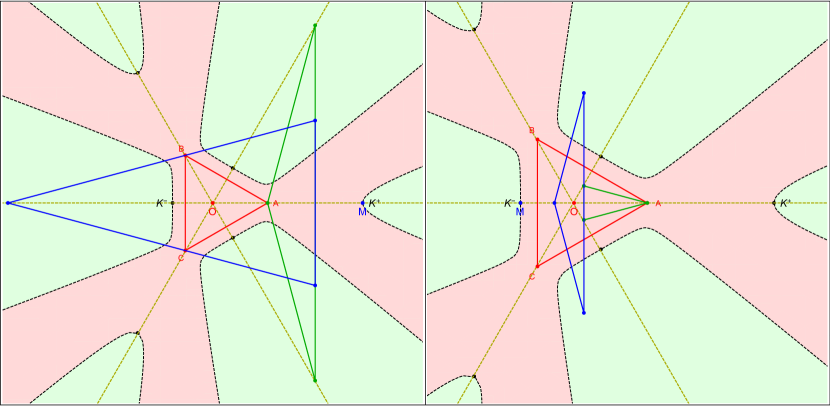
Figure 11. Left: starting with an equilateral $ABC$, when $M$ is at $K^{+}=(1+\sqrt{3},0)$, repeated applications of the circumcenter map will cycle indefinitely through the 3 canonical triangles shown (red, green, blue). Right: With $M=K^{-}=(1-\sqrt{3},0)$, the sequence is also 3-periodic, and the canonical triangles obtained are as shown.

Referring to Figure 12, it can be shown that:

Remark 3.

When $M$ is the centroid of $\mathcal{R}$, repeated applications of the circumcenter are 2-periodic, where the first triangle is $\mathcal{R}$ and the second one is a reflection of $\mathcal{R}$ about said centroid.

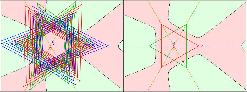
Figure 12. Left: 36 iterations of the circumcenter map with $M$ close to the centroid $O$ of the starting equilateral, resulting in a sequence which is slightly expanding. Right: If $M=O$, the sequence becomes 2-periodic, containing only the original $ABC$ (blue) and its reflection about $O$ (green).

The case of a square

Let $\mathcal{Q}=ABCD$ be a square with with vertices $A=(1,0)$, $B=(0,1)$, $C=(-1,0)$, $D=(0,-1)$. Let $\mathcal{Q}^{\prime}=\mathcal{C}_{M}^{4}(\mathcal{Q})$, with $M=(x_{m},y_{m})$. Via CAS, we obtain the following propositions.

Proposition 8.

Starting from the square $\mathcal{Q}$, $s=1$ occurs when $M=(x_{m},y_{m})$ satisfies:

$$\;\;\;\;15x_{m}^{8}-68x_{m}^{6}y_{m}^{2}+90x_{m}^{4}y_{m}^{4}-68x_{m}^{2}y_{m}^{6}+15y_{m}^{8}-64x_{m}^{6}+64x_{m}^{4}y_{m}^{2}+$$

$$64x_{m}^{2}y_{m}^{4}-64y_{m}^{6}+98x_{m}^{4}+52x_{m}^{2}y_{m}^{2}+98y_{m}^{4}-64x_{m}^{2}-64y_{m}^{2}+15=0$$

Proposition 9.

Starting from the square $\mathcal{Q}$, $\alpha=0$ when $M=(x_{m},y_{m})$ satisfies:

$$x_{m}y_{m}(x_{m}^{2}-y_{m}^{2})=0$$

4. Regular polygons, $n\geq 3$

In this section we assume $\mathcal{P}$ is a regular $n$-gon, $n{\geq}3$. Without loss of generality, let the centroid $O=(0,0)$ and the first vertex $P_{1}=(1,0)$. Figure 13 illustrates the partitioning of the plane into area-contracting and area-expanding regions by $n$ applications of the map, for $n=3,4,5,6$.

Proposition 10.

As $M$ approaches a sideline of $\mathcal{P}$, $s$ approaches infinity.

The proof below was kindly contributed by a referee.

Proof.

If $M$ is on a sideline of $\mathcal{P}$, say $P_{i}P_{i+1}$, then $P_{i}^{\prime}$ is at infinity (since $P_{i}^{\prime}$ is the intersection of the bisectors $MP_{i}$ and $MP_{i+1}$), but the rest of the vertices $P_{j}^{\prime}$ are finite. If a polygon $\mathcal{P}$ has a vertex at infinity, it will remain at infinity under the map $\mathcal{C}_{M}$. ∎

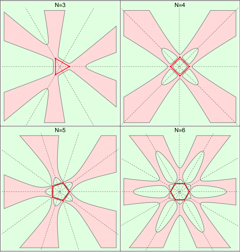
Figure 13. Area contraction (green) and expansion (red) regions for the circumcenter map applied to a regular triangle (top left), square (top right), pentagon (bottom left) and hexagon (bottom right). Notice that in all but in the $n=3$, an area contracting region exists interior to the original polygon. Also shown are the zero-rotation lines (dashed black).

Let $\mathcal{P}^{\prime}=\mathcal{C}_{M}^{n}(\mathcal{P})$. Let $\alpha$ be the angle of rotation of the similarity that takes $\mathcal{P}$ to $\mathcal{P}^{\prime}$.

Conjecture 1.

The locus of $M$ such that $\alpha=0$ is the union of $n$ lines along directions $k\pi/n$, $k=0,\ldots,n-1$.

To facilitate region counting, in Figure 14 the plane is compactified into a single hemisphere, via stereographic projection. Table 1 shows the counts of area-contracting regions. This suggests:

n	interior	non-compact	compact	total
3	0	2n	0	2n
4	1	n	n	1+2n
5	1	2n	n	1+3n
6	1	n	2n	1+3n
7	1	2n	2n	1+4n
8	1	n	3n	1+4n
9	1	2n	3n	1+5n
10	1	n	4n	1+5n
11	1	2n	4n	1+6n

Table 1. Region count according to Figure 14

.

Conjecture 2.

There is a single connected area-expanding region. Let $k$ denote the number of area-contracting connected regions. Then:

$$k=\begin{cases}\;\mbox{odd}~{}n:\;\;r^{*}+n(n+1)/2\\ \mbox{even}~{}n:~{}1+n^{2}/2\\ \end{cases}$$

where $r^{*}=0$ if $n=3$, and $1$ otherwise.

Experiments suggest:

Conjecture 3.

Given an $n$, the number of area-contracting regions for a simple $n$-gon $\mathcal{Q}$ (no self-intersections), is maximal if $\mathcal{Q}$ is regular.

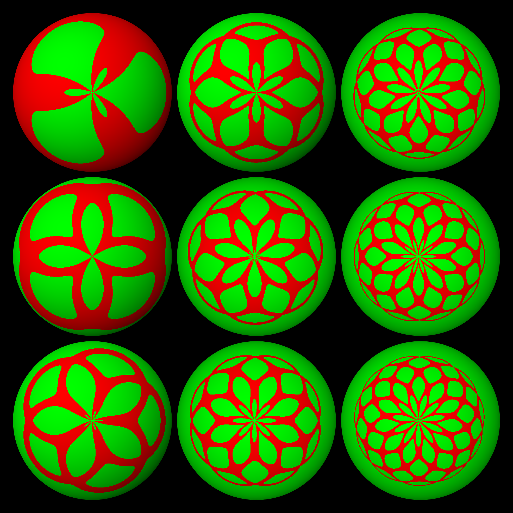
Figure 14. Area-expansion (red) and area-contraction (green) regions for regular $n$-gons, compactified (via stereographic projection) to a single hemisphere; the south pole (center) is “infinity”. From top-to-bottom, left-to-right, $N=3,\ldots,11$. For interactive examples, see bit.ly/3Pl2tmz and [4].

5. conclusion

A video walk-through of our experiments appears in [6]. A gallery of interactive experiments appears in bit.ly/3Pl2tmz with implementation details in [4].

See [4] for a gallery of interactive experiments with the circumcenter map.

The circumcenter map can be generalized to the $X_{k}$-map, where $X_{k}$ is some triangle center (see [3]). For example, the $X_{2}$-map sends a polygon to one with vertices at the barycenters of $MP_{i}P_{i+1}$ of vertices of a given polygon. In such a case, an iteration produces a sequence of ever-shrinking polygons which converges to $M$. If the starting polygon is a triangle, a few notable cases include: (i) the $X_{4}$-map (orthocenter) is area preserving for all $M$, and the sequence of triangles tends to an infinite line; (ii) the $X_{16}$-map (second isodynamic point) induces regions of the plane such that 3 applications of the map are the identity (no rotation and no scaling), see [7]. A question not addressed here, is whether a certain $X_{k}$-map is integrable in the sense of [1, 5].

Appendix A Explicit Circumcenter Map

Let $\mathcal{P}$ be a generic $n$-gon with vertices $(x_{i},y_{i})$, $i=1,\ldots,n$, and $M=(x_{m},y_{m})$. The $M$-circumcenter map $\mathcal{C}_{M}(\mathcal{P})$ yields a new polygon with vertices $(p_{i},q_{i})$ given by:

$$p_{i} =\frac{(y_{i+1}-y_{m})y_{i}^{2}+\rho_{i}y_{i}+y_{i+1}^{2}y_{m}+(x_{i}^{2}-x_{m}^{2}-y_{m}^{2})y_{i+1}+(x_{i+1}^{2}-x_{i}^{2})y_{m}}{2(x_{m}-x_{i+1})y_{i}+2(x_{i}-x_{m})y_{i+1}+2(x_{i+1}-x_{i})y_{m}}$$

$$q_{i} =\frac{(x_{m}-x_{i+1})x_{i}^{2}-\rho_{i}x_{i}-x_{i+1}^{2}x_{m}+(x_{m}^{2}+y_{m}^{2}-y_{i}^{2})x_{i+1}+x_{m}(y_{i}^{2}-y_{i+1}^{2})}{2(y_{i+1}-y_{m})x_{i}+2(y_{m}-y_{i})x_{i+1}+2(y_{i}-y_{i+1})x_{m}}$$

where $\rho_{i}=|M|^{2}-|B|^{2}=x_{m}^{2}+y_{m}^{2}-x_{i+1}^{2}-y_{i+1}^{2}$.

Likewise, the inverse the $M$-circumcenter map $\mathcal{C}_{M}^{-1}(\mathcal{P})$ yields a new polygon with vertices $(u_{i},v_{i})$ given by:

$$u_{i} =\frac{r_{i}^{\prime}x_{m}+2(y_{i+1}-y_{i})(x_{i+1}-x_{i})y_{m}+2(y_{i+1}-y_{i})(x_{i}y_{i+1}-x_{i+1}y_{i})}{r_{i}}$$

$$v_{i} =\frac{-r_{i}^{\prime}y_{m}+2(y_{i+1}-y_{i})(x_{i+1}-x_{i})x_{m}-2(x_{i+1}-x_{i})(x_{i}y_{i+1}-x_{i+1}y_{i})}{r_{i}}$$

where $r_{i}=(x_{i+1}-x_{i})^{2}+(y_{i+1}-y_{i})^{2}$, and $r_{i}^{\prime}=(x_{i+1}-x_{i})^{2}-(y_{i+1}-y_{i})^{2}$.

References

[1]Arnold, M., Fuchs, D., and Tabachnikov, S.A family of integrable transformations of centroaffine polygons:
geometrical aspects, 12 2021, arXiv:2112.08124.
[2]Johnson, R. A.The theory of similar figures.
Amer. Math. Monthly 25, 3 (1918), 108–113.
[3]Kimberling, C.Triangle centers as functions.
Rocky Mountain J. Math. 23, 4 (1993), 1269–1286.
[4]McDonald, N.Exploring the circumcenter map: GPU acceleration.
In Nick’s Blog. nickcmd.org, 2022.
https://bit.ly/3Pl2tmz.
[5]Ovsienko, V., Schwartz, R., and Tabachnikov, S.The pentagram map: A discrete integrable system.
S. Commun. Math. Phys. 299 (2010), 409–446.
[6]Reznik, D.Dynamics of the circumcenter map: Periodicity, stability, converging,
and diverging zones.
YouTube, 3 2021.
https://youtu.be/y6F8SmA67pw.
[7]Reznik, D.Identity zones of the isodynamic map.
Wolfram Communities, 4 2021.
[8]Reznik, D., and Garcia, R.Dynamics of the circumcenter map.
Wolfram Communities, 4 2021.
[9]Stewart, B. M.Cyclic properties of Miquel polygons.
Am. Math. Monthly 47, 7 (1940), 462–466.
[10]Stupel, M.A triangle “broken” into four triangles – the special status of
the central triangle.
J. for Geom. and Graphics 22, 2 (2018), 253–256.