One-Nearest-Neighbor Search is All You Need
for Minimax Optimal Regression and Classification

Abstract

Recently, Qiao, Duan, and Cheng (2019) proposed a distributed nearest-neighbor classification method, in which a massive dataset is split into smaller groups, each processed with a $k$-nearest-neighbor classifier, and the final class label is predicted by a majority vote among these groupwise class labels. This paper shows that the distributed algorithm with $k=1$ over a sufficiently large number of groups attains a minimax optimal error rate up to a multiplicative logarithmic factor under some regularity conditions, for both regression and classification problems. Roughly speaking, distributed 1-nearest-neighbor rules with $M$ groups has a performance comparable to standard $\Theta(M)$-nearest-neighbor rules. In the analysis, alternative rules with a refined aggregation method are proposed and shown to attain exact minimax optimal rates.

1 Introduction

Arguably being the most primitive, yet powerful nonparametric approaches for various statistical problems, the $k$-nearest-neighbor ($k$-NN) based algorithms have been one of the essential toolkits in data science since their inception. They have been extensively studied and analyzed over several decades for canonical statistical procedures including classification (Fix & Hodges, 1951; Cover & Hart, 1967), regression (Cover, 1968a, b), density estimation (Loftsgaarden & Quesenberry, 1965; Fukunaga & Hostetler, 1973; Mack & Rosenblatt, 1979), and density functional estimation (Kozachenko & Leonenko, 1987; Leonenko et al., 2008). They are attractive even in this modern age due to their simplicity, decent performance, and rich understanding of their statistical properties.

There exist, however, clear limitations that hinder their wider deployment in practice. First, and most importantly, standard $k$-NN based algorithms are often deemed to be inherently infeasible for large-scale data, as they need to store and process the entire data in a single machine for NN search. Second, though the number of neighbors $k$ needs to grow to infinity in the sample size to achieve statistical consistency in general for such procedures (Biau & Devroye, 2015), small $k$ is highly preferred in practice to avoid possibly demanding time complexity of large-$k$-NN search; see Section 3.1 for an in-depth discussion.

Recently, specifically for regression and classification, a few ensemble based methods (Xue & Kpotufe, 2018; Qiao et al., 2019; Duan et al., 2020) have been proposed aiming to reduce the computational complexity while achieving the accuracy of the optimal standard $k$-NN regression and classification rules; however, theoretical guarantees of those solutions still require large-$k$-NN search. Xue & Kpotufe (2018) proposed an idea dubbed as denoising, which is to draw (multiple) subsample(s) and preprocess them with the standard large-$k$-NN rule over the entire data in the training phase, so that the $k$-NN information can be hashed effectively by 1-NN searches in the testing phase. Though the resulting algorithm is provably optimal with a small statistical overhead, the denoising step may still suffer prohibitively large complexity for large $N$ and/or large $k$ in principle. More recently, to address the computational and storage complexity of the standard $k$-NN classifier with large $N$, Qiao et al. (2019) proposed the bigNN classifier, which splits data into subsets, applies the standard $k$-NN classifier to each, and aggregates the labels by a majority vote. This ensemble method works without any coordination among data splits, and thus they naturally fit to large-scale data which may be inherently stored and processed in distributed machines. However, they showed its minimax optimality only when both the number of splits $M$ and the base $k$ increase as the sample size $N$ increases but only a strictly suboptimal guarantee for fixed $k$. Only with the optimality for increasingly large $k$, they suggested to use the bigNN classifier in the preprocessing phase of the denoising framework. A more recent work (Duan et al., 2020) on optimally weighted version of the bigNN classifier still assumes increasingly large $k$.

In this paper, we complete the missing theory for small $k$ and show that the bigNN classifier with $k=1$ suffices for minimax rate-optimal classification. More generally, we analyze a variant of the bigNN classifier, called the $M$-split $k$-NN classifier, which is defined as the majority vote over the total $kM$ nearest-neighbor labels obtained after running $k$-NN search over the $M$ data splits. Roughly put, we show that the $M$-split $k$-NN classification rule behaves almost equivalently to the standard $\Theta(M)$-NN rules, for any fixed $k\geq 1$. In particular, the $M$-split 1-NN rule, equivalent to the bigNN classifier with $k=1$, is shown to attain a minimax optimal rate up to logarithmic factors under smooth measure conditions. We also provide a minimax-rate-optimal guarantee for regression task with an analogously defined $M$-split $k$-NN regression rule.

Albeit both the algorithm and analysis are simple in nature, the practical implication of theoretical guarantees provided herein together with the divide-and-conquer framework is significant: while running faster than the standard 1-NN rules by processing smaller data with small-$k$-NN search in parallel, the $M$-split $k$-NN rules can achieve the same statistical guarantee of the optimal standard $k$-NN rules run over the entire dataset. Moreover, when deploying the rules in practice, we only need to tune the number of splits $M$ while fixing $k$, say, simply $k=1$. We experimentally demonstrate that the split 1-NN rules indeed perform on par with the optimal standard $k$-NN rules as expected by theory, while running faster than the standard 1-NN rules.

The key technique in our analysis is to analyze intermediate rules that selectively aggregates the small-$k$-NN estimates from each data split based on the $k$-th-NN distances from a query point. The intuition is that these intermediate rules which average only neighbors close enough to a query point exactly behave like a standard $\Theta(M)$-NN rule for any fixed $k$. We establish the performance of the $(M,k)$-NN rules by showing that its performance is approximated by the intermediate rules, with a small (logarithmic) approximation overhead in rates. Indeed, these intermediate rules attain exact minimax optimal rates for respective problems at the cost of additional complexity for ordering the NN distances.

Organization

The rest of the paper is organized as follows. Section 2 presents the main results with the formal definition of the split NN rules and their theoretical guarantees. In Section 3, we discuss computational complexity of the standard $k$-NN algorithms and the $M$-split $k$-NN rules, a refined aggregation scheme that removes the logarithmic factors in the previous guarantees, and a comparison to the bigNN classifier and its theoretical guarantee of (Qiao et al., 2019). We demonstrate the convergence rates of the split NN rules and their practicality over the standard $k$-NN rules with experimental results in Section 4. Due to the space limit, we discuss other related work and present all proofs in Appendix.

2 Main Results

Let $(\mathcal{X},\rho)$ be a metric space and let $\mathcal{Y}$ be the outcome (or label) space, i.e., $\mathcal{Y}\subseteq\mathbb{R}$ for regression and $\mathcal{Y}=\{0,1\}$ for binary classification. We denote by $\operatorname{\mathsf{P}}$ a joint distribution over $\mathcal{X}\times\mathcal{Y}$, by $\mu$ the marginal distribution on $\mathcal{X}$, and by $\eta$ the regression function $\eta(x)=\mathbb{E}[Y\mathchoice{\mspace{1.0mu}|\mspace{1.0mu}}{|}{|}{|}X=x]$.

We denote an open ball of radius $r$ centered at $x\in\mathcal{X}$ by $B^{o}(x,r)\mathrel{\mathop{\mathchar 58\relax missing}}=\{x^{\prime}\in\mathcal{X}\mathchoice{\colon}{\colon}{\mathchar 58\relax\mspace{1.0mu}}{\mathchar 58\relax}\rho(x,x^{\prime})<r\}$ and the closed ball by $B(x,r)\mathrel{\mathop{\mathchar 58\relax missing}}=\overline{B^{o}(x,r)}$. The support of a measure $\mu$ is denoted as $\textnormal{supp}(\mu)\mathrel{\mathop{\mathchar 58\relax missing}}=\{x\in\mathcal{X}\mathchoice{\colon}{\colon}{\mathchar 58\relax\mspace{1.0mu}}{\mathchar 58\relax}\mu(B^{o}(x,r))>0,~{}\forall r>0\}$.

Given sample $\mathcal{D}=({\mathbf{X}},\mathbf{Y})=\{(X_{i},Y_{i})\}_{i=1}^{N}$ and a point $x\in\mathbb{R}^{d}$, we use $X_{(k)}(x;{\mathbf{X}})$ to denote the $k$-th-nearest neighbor of $x$ from the sample instances ${\mathbf{X}}=X_{1\mathchar 58\relax N}$ and use $Y_{(k)}(x;\mathcal{D})$ to denote the corresponding $k$-th-NN label among $\mathbf{Y}=Y_{1\mathchar 58\relax N}$; any tie is broken arbitrarily. The $k$-th-NN distance of $x$ is denoted as $r_{k}(x;{\mathbf{X}})\mathrel{\mathop{\mathchar 58\relax missing}}=\rho(x,X_{(k)}(x;{\mathbf{X}}))$ for $k\leq N$. We will omit the underlying data $\mathcal{D}$ or ${\mathbf{X}}$ whenever it is clear from the context.

Throughout in the paper, we use $N$, $M$, and $n=N/M$ to denote the size of the entire data $\mathcal{D}$, the number of data splits, and the size of each data split, respectively, assuming that $M$ divides $N$.

2.1 Regression

2.1.1 Problem Setting

Given paired data $\mathcal{D}=\{(X_{i},Y_{i})\}_{i=1}^{N}$ drawn independently from $\operatorname{\mathsf{P}}$, the goal of regression is to design an estimator $\hat{\eta}=\hat{\eta}(\cdot;\mathcal{D})\mathchoice{\colon}{\colon}{\mathchar 58\relax\mspace{1.0mu}}{\mathchar 58\relax}\mathcal{X}\to\mathcal{Y}$ based on the data such that the estimate $\hat{\eta}(x)$ is close to the conditional expectation $\eta(x)=\mathbb{E}[Y\mathchoice{\mspace{1.0mu}|\mspace{1.0mu}}{|}{|}{|}X=x]$, where the closeness between $\eta$ and $\hat{\eta}$ is typically measured by the $l_{p}$-norm under $\mu$, $\|\hat{\eta}-\eta\|_{p}\mathrel{\mathop{\mathchar 58\relax missing}}=(\int\mathchoice{\mspace{1.0mu}|\mspace{1.0mu}}{|}{|}{|}\hat{\eta}(x)-\eta(x)\mathchoice{\mspace{1.0mu}|\mspace{1.0mu}}{|}{|}{|}^{p}\mu(\mathop{}\!\mathrm{d}x))^{1/p}$ for $p=1,2,$ or the sup norm $\|\hat{\eta}-\eta\|_{\infty}\mathrel{\mathop{\mathchar 58\relax missing}}=\sup_{x\in\mathcal{X}}\mathchoice{\mspace{1.0mu}|\mspace{1.0mu}}{|}{|}{|}\hat{\eta}(x)-\eta(x)\mathchoice{\mspace{1.0mu}|\mspace{1.0mu}}{|}{|}{|}$.

2.1.2 The Proposed Rule

Given a query $x\in\mathcal{X}$, we first recall that the standard $k$-NN regression rule outputs the average of the $k$-NN labels, i.e.,

$$\hat{\eta}^{(k)}(x;\mathcal{D})\mathrel{\mathop{\mathchar 58\relax missing}}=\frac{1}{k}\sum_{i=1}^{k}Y_{(i)}(x;\mathcal{D}).$$

Instead of running $k$-NN search over the entire data, given the number of splits $M\geq 1$, we first split the data $\mathcal{D}$ of size $N$ into $M$ subsets of equal size at random. Let $\mathcal{P}=\{\mathcal{D}_{1},\ldots,\mathcal{D}_{M}\}$ denote the random subsets, where $\mathcal{D}_{m}$ corresponds to the $m$-th split. After finding $k$-NN labels for each data split, the $M$-split $k$-NN (or $(M,k)$-NN in short) regression rule is defined as the average of all $kM$ of returned labels, i.e.,

$$\tilde{\eta}_{M}^{(k)}(x)\mathrel{\mathop{\mathchar 58\relax missing}}=\tilde{\eta}^{(k)}(x;\mathcal{P})\mathrel{\mathop{\mathchar 58\relax missing}}=\frac{1}{M}\sum_{m=1}^{M}\hat{\eta}^{(k)}(x;\mathcal{D}_{m}).$$ (2.1)

2.1.3 Performance Guarantees

We claim that the proposed $(M,k)$-NN regression rule for any fixed $k\geq 1$ is nearly optimal in terms of error rate under a standard regularity condition. For a formal statement, we borrow some standard assumptions on the metric measure space in the literature on analyzing $k$-NN algorithms (Dasgupta & Kpotufe, 2019).

Assumption 2.1 (Doubling and homogeneous measure).

The measure $\mu$ on metric space $(\mathcal{X},\rho)$ is doubling with exponent $d$, i.e., for any $x\in\textnormal{supp}(\mu)$ and $r>0$,

$$\mu(B^{o}(x,r))\leq 2^{d}\mu(B^{o}(x,r/2)).$$

The measure $\mu$ is $(C_{d},d)$-homogeneous, i.e., for some $C_{d}>0$ for any $x\in\textnormal{supp}(\mu)$ and $r>0$,

$$\mu(B^{o}(x,r))\geq\min\{C_{d}r^{d},1\}.$$

Note that a measure $\mu$ is homogeneous if $\mu$ is doubling and $\textnormal{supp}(\mu)$ is bounded. The doubling exponent $d$ can be interpreted as an intrinsic dimension of a measure space.

Assumption 2.2 (Hölder continuity).

The conditional expectation function $\eta(x)=\mathbb{E}[Y\mathchoice{\mspace{1.0mu}|\mspace{1.0mu}}{|}{|}{|}X=x]$ is $(\alpha_{\mathrm{H}},A)$-Hölder continuous for some $0<\alpha_{\mathrm{H}}\leq 1$ and $A>0$ in metric space $(\mathcal{X},\rho)$, i.e., for any $x,x^{\prime}\in\mathcal{X}$,

$$\mathchoice{\mspace{1.0mu}|\mspace{1.0mu}}{|}{|}{|}\eta(x)-\eta(x^{\prime})\mathchoice{\mspace{1.0mu}|\mspace{1.0mu}}{|}{|}{|}\leq A\rho^{\alpha_{\mathrm{H}}}(x,x^{\prime}).$$

Assumption 2.3 (Bounded conditional expectation and variance).

The conditional expectation function $\eta(x)=\mathbb{E}[Y\mathchoice{\mspace{1.0mu}|\mspace{1.0mu}}{|}{|}{|}X=x]$ and the conditional variance function $v(x)\mathrel{\mathop{\mathchar 58\relax missing}}=\mathop{\rm Var}\nolimits(Y\mathchoice{\mspace{1.0mu}|\mspace{1.0mu}}{|}{|}{|}X=x)$ are bounded, i.e., $\sup_{x\in\mathcal{X}}\mathchoice{\mspace{1.0mu}|\mspace{1.0mu}}{|}{|}{|}\eta(x)\mathchoice{\mspace{1.0mu}|\mspace{1.0mu}}{|}{|}{|}<\infty$ and $\sup_{x\in\mathcal{X}}v(x)<\infty$.

The following condition is borrowed from (Xue & Kpotufe, 2018) to establish a high-probability bound.

Assumption 2.4.

The collection of closed balls in $\mathcal{X}$ has finite VC dimension $\mathcal{V}$ and the outcome space $\mathcal{Y}\subset\mathbb{R}$ is contained in a bounded interval of length $l_{Y}$.

The main goal of this paper is to demonstrate that the distributed $(M,k)$-NN rules can attain almost statistically equivalent performance to the optimal $k$-NN rules. Hence, our statements in what follows are written in parallel to the known results for the standard $k$-NN rules, to which we include the pointers after cf. for the interested reader. For example, the following statement is new and we refer to (Dasgupta & Kpotufe, 2019) for an analogous statement for the standard $k$-NN regression algorithm.

Theorem 2.1 (cf. (Dasgupta & Kpotufe, 2019, Theorem 1.3)).

Suppose that Assumptions 2.1 and 2.2 hold. Let $k\geq 1$ be fixed.

1. If Assumption 2.3 holds and the support of $\mu$ is bounded, for any $M\leq N$ such that $N/M\geq k$, we have

   $$\mathbb{E}_{\mathcal{P}}\|\tilde{\eta}_{M}^{(k)}-\eta\|_{2}\leq C_{1}\Bigl{(}\Bigl{(}\frac{M}{N}\log\frac{M}{(\log M)^{1.01}}\Bigr{)}^{\frac{\alpha_{\mathrm{H}}}{d}}+\sqrt{\frac{(\log M)^{1.01}}{M}}\Bigr{)}.$$

2. If Assumption 2.4 holds, for any $0<\delta<1$, if $M\geq 16\log\frac{1}{\delta}$, then with probability at least $1-\delta$ over $\mathcal{P}$, we have

   $$\|\tilde{\eta}_{M}^{(k)}-\eta\|_{\infty}\leq C_{2}\Bigl{(}\Bigl{(}\frac{M}{N}\log N\Bigr{)}^{\frac{\alpha_{\mathrm{H}}}{d}}+\sqrt{\frac{1}{M}\log\frac{N}{\delta}}\Bigr{)}.$$

In particular, $C_{1}$ and $C_{2}$ are constants and independent of the ambient dimension $D$.

Remark 2.1 (Minimax optimality).

If we set $M=\tilde{\Theta}(N^{2\alpha_{\mathrm{H}}/(2\alpha_{\mathrm{H}}+d)})$, Theorem 2.1 gives

$$\mathbb{E}_{\mathcal{P}}\|\tilde{\eta}_{M}^{(k)}-\eta\|_{2} =\tilde{O}(N^{-\alpha_{\mathrm{H}}/(2\alpha_{\mathrm{H}}+d)})\text{ and}$$

$$\|\tilde{\eta}_{M}^{(k)}-\eta\|_{\infty} =\tilde{O}(N^{-\alpha_{\mathrm{H}}/(2\alpha_{\mathrm{H}}+d)})\text{ with high probability},$$

where $\tilde{O}(\cdot)$ hides any logarithmic multiplicative terms. This rate is known to be minimax optimal under the Hölder continuity of order $\alpha_{\mathrm{H}}$; for the standard $k$-NN regression algorithm, this rate optimality is attained for $k=\Theta(N^{2\alpha_{\mathrm{H}}/(2\alpha_{\mathrm{H}}+d)})$ (Dasgupta & Kpotufe, 2019; Xue & Kpotufe, 2018). In this view, the $(M,k)$-NN regression algorithm attains the performance of the standard $\Theta(M)$-NN regression algorithm for any fixed $k$.

2.2 Classification

2.2.1 Problem Setting

We consider the binary classification with $\mathcal{Y}=\{0,1\}$. Given paired data $\mathcal{D}=\{(X_{i},Y_{i})\}_{i=1}^{N}$ drawn independently from $\operatorname{\mathsf{P}}$, the goal of binary classification is to design a (data-dependent) classifier ${\hat{g}}(\cdot;\mathcal{D})\mathchoice{\colon}{\colon}{\mathchar 58\relax\mspace{1.0mu}}{\mathchar 58\relax}\mathcal{X}\to\mathcal{Y}$ such that it minimizes the classification error $\mathsf{P}({\hat{g}}(X;\mathcal{D})\neq Y)$. For a classifier ${\hat{g}}\mathchoice{\colon}{\colon}{\mathchar 58\relax\mspace{1.0mu}}{\mathchar 58\relax}\mathcal{X}\to\mathcal{Y}$, we define its pointwise risk at $x\in\mathcal{X}$ as $R({\hat{g}};x)\mathrel{\mathop{\mathchar 58\relax missing}}=\mathsf{P}(Y\neq{\hat{g}}(x)\mathchoice{\mspace{1.0mu}|\mspace{1.0mu}}{|}{|}{|}X=x)$, and define the (expected) risk as $R({\hat{g}})\mathrel{\mathop{\mathchar 58\relax missing}}=\mathsf{P}(Y\neq{\hat{g}}(X))$. Let $g(x)$ denote the Bayes-optimal classifier, i.e., $g(x)\mathrel{\mathop{\mathchar 58\relax missing}}=\mathds{1}\{\eta(x)\geq 1/2\}$ for all $x\in\mathcal{X}$, and let $R^{*}(x)\mathrel{\mathop{\mathchar 58\relax missing}}=R(g;x)=\eta(x)\wedge(1-\eta(x))$ and $R^{*}\mathrel{\mathop{\mathchar 58\relax missing}}=R(g)$ denote the pointwise-Bayes risk and the (expected) Bayes risk, respectively. The canonical performance measure of a classifier ${\hat{g}}$ is its excess risk $R({\hat{g}})-R^{*}$.

Another important performance criterion is the classification instability proposed by (Sun et al., 2016), which quantifies a stablility of a classification procedure with respect to independent realizations of training data. Given $N\in\mathbb{N}$, with a slight abuse of notation, denote ${\hat{g}}$ as a classification procedure $\mathcal{D}\mapsto{\hat{g}}(\cdot;\mathcal{D})$ that maps a dataset $\mathcal{D}$ of size $N$ to a classifier ${\hat{g}}(\cdot;\mathcal{D})$. The classification instability of the classification procedure is defined as

$$\mathop{\rm CIS}\nolimits_{N}({\hat{g}})\mathrel{\mathop{\mathchar 58\relax missing}}=\mathbb{E}[\mathsf{P}({\hat{g}}(X;\mathcal{D})\neq{\hat{g}}(X;\mathcal{D}^{\prime})\mathchoice{\mspace{1.0mu}|\mspace{1.0mu}}{|}{|}{|}\mathcal{D},\mathcal{D}^{\prime})],$$

where $\mathcal{D}$ and $\mathcal{D}^{\prime}$ are independent, i.i.d. data of size $N$.

2.2.2 The Proposed Rule

The standard $k$-NN classifier is defined as the plug-in classifier of the standard $k$-NN regression estimate:

$${\hat{g}}_{k}(x;\mathcal{D})\mathrel{\mathop{\mathchar 58\relax missing}}=\mathds{1}\Bigl{(}\hat{\eta}^{(k)}(x;\mathcal{D})\geq\frac{1}{2}\Bigr{)}.$$

It can be equivalently viewed as the majority vote over the $k$-NN labels given a query.

Similarly, we define the $(M,k)$-NN classification rule as the plug-in classifier of the $(M,k)$-NN regression rule:

$${\tilde{g}}_{M}^{(k)}(x)\mathrel{\mathop{\mathchar 58\relax missing}}={\tilde{g}}^{(k)}(x;\mathcal{P})\mathrel{\mathop{\mathchar 58\relax missing}}=\mathds{1}\Bigl{(}\tilde{\eta}^{(k)}(x;\mathcal{P})\geq\frac{1}{2}\Bigr{)}.$$

2.2.3 Performance Guarantees

As shown in the previous section for regression, we can show that the proposed $(M,k)$-NN classifier behaves nearly identically to the standard $\Theta(M)$-NN rules for any fixed $k\geq 1$. Here, we focus on guarantees on rates of excess risk and classification instability, but the asymptotic Bayes consistency can be also established under a mild condition; see Theorem B.13 in Appendix.

To establish rates of convergence for classification, we recall the following notion of smoothness for the conditional probability $\eta(x)=\operatorname{\mathsf{P}}(Y=1\mathchoice{\mspace{1.0mu}|\mspace{1.0mu}}{|}{|}{|}X=x)$ defined in (Chaudhuri & Dasgupta, 2014) that takes into account the underlying measure $\mu$ to better capture the nature of classification than the standard Hölder continuity in Assumption 2.2.

Assumption 2.5 (Smoothness).

For $\alpha\in(0,1]$ and $A>0$, $\eta(x)$ is $(\alpha,A)$-smooth in metric measure space $(\mathcal{X},\rho,\mu)$, i.e., for all $x\in\textnormal{supp}(\mu)$ and $r>0$,

$$\lvert\eta(B(x,r))-\eta(x)\rvert\leq A\mu^{\alpha}(B^{o}(x,r)).$$

The following condition on the behavior of the measure $\mu$ around the decision boundary of $\eta$ is a standard assumption to establish a fast rate of convergence (Audibert et al., 2007).

Assumption 2.6 (Margin condition).

For $\beta\geq 0$, $\eta$ satisfies the $\beta$-margin condition in $(\mathcal{X},\rho,\mu)$, i.e., there exists a constant $C>0$ such that

$$\mu(\mathop{}\!\partial\eta_{\Delta})\leq C\Delta^{\beta},$$

where $\mathop{}\!\partial\eta_{\Delta}\mathrel{\mathop{\mathchar 58\relax missing}}=\{x\in\textnormal{supp}(\mu)\mathchoice{\colon}{\colon}{\mathchar 58\relax\mspace{1.0mu}}{\mathchar 58\relax}\mathchoice{\mspace{1.0mu}|\mspace{1.0mu}}{|}{|}{|}\eta(x)-1/2\mathchoice{\mspace{1.0mu}|\mspace{1.0mu}}{|}{|}{|}\leq\Delta\}$ denotes the decision boundary with margin $\Delta\in(0,1/2]$.

The following statement is new.

Theorem 2.2 (cf. (Chaudhuri & Dasgupta, 2014, Theorem 4)).

Under Assumptions 2.5 and 2.6, the following statements hold for any fixed $k\geq 1$, where $M_{o}$, $C_{o}$, and $C_{o}^{\prime}$ are constants depending on $k,\alpha,\beta,$ and $C$.

1. Pick any $\delta\in(0,1)$ and $M_{o}>0$ such that $M=M_{o}N^{\frac{2\alpha}{2\alpha+1}}(\log\frac{1}{\delta})^{\frac{1}{2\alpha+1}}\leq N$. With probability at least $1-\delta$ over $\mathcal{P}$,

   $$\mathsf{P}({\tilde{g}}_{M}^{(k)}(x)\neq g(X)\mathchoice{\mspace{1.0mu}|\mspace{1.0mu}}{|}{|}{|}\mathcal{P})\leq\delta+C_{o}\Bigl{(}\frac{1}{N}\log\frac{1}{\delta}\Bigr{)}^{\frac{\beta\alpha}{2\alpha+1}}\Bigl{(}\log\frac{N}{\log\frac{1}{\delta}}\Bigr{)}^{\beta\alpha}.$$

2. Pick any $M_{o}\in(0,N^{\frac{1}{2\alpha+1}}]$ and set $M=M_{o}N^{\frac{2\alpha}{2\alpha+1}}\leq N$. Then

   $$\mathbb{E}_{\mathcal{P}}[R({\tilde{g}}_{M}^{(k)})]-R^{*} \leq C_{o}^{\prime}\Bigl{(}\frac{(\log N)^{\alpha\vee\frac{1}{2}}}{N^{\frac{\alpha}{2\alpha+1}}}\Bigr{)}^{\beta+1}\quad\text{and}\quad$$

   $$\mathop{\rm CIS}\nolimits_{N}({\tilde{g}}_{M}^{(k)}) \leq C_{o}^{\prime\prime}\Bigl{(}\frac{(\log N)^{\alpha\vee\frac{1}{2}}}{N^{\frac{\alpha}{2\alpha+1}}}\Bigr{)}^{\beta}.$$

Remark 2.2 (Minimax optimality).

Suppose that $\eta$ is $(\alpha_{\mathrm{H}},A)$-Hölder continuous and $\mu$ has a density with respect to Lebesgue measure that is strictly bounded away from zero on its support. Then, by (Chaudhuri & Dasgupta, 2014, Lemma 2), $\eta$ is $(\frac{\alpha_{\mathrm{H}}}{d},A)$-smooth. Hence, if we set $M=\tilde{\Theta}(N^{2\alpha_{\mathrm{H}}/(2\alpha_{\mathrm{H}}+d)})$ in Theorem 2.2(b) as in Remark 2.1, we have

$$\mathbb{E}_{\mathcal{P}}[R({\tilde{g}}_{M}^{(k)})]-R^{*} =\tilde{O}(N^{-(\beta+1)\alpha_{\mathrm{H}}/(2\alpha_{\mathrm{H}}+d)})\quad\text{and}$$

$$\mathop{\rm CIS}\nolimits_{N}({\tilde{g}}_{M}^{(k)}) =\tilde{O}(N^{-\beta\alpha_{\mathrm{H}}/(2\alpha_{\mathrm{H}}+d)}),$$

which are known to be minimax optimal under the Hölder continuity assumption (Chaudhuri & Dasgupta, 2014; Sun et al., 2016). In parallel to Remark 2.1, the standard $k$-NN classifier is known to achieve these rates for $k=\Theta(N^{2\alpha_{\mathrm{H}}/(2\alpha_{\mathrm{H}}+d)})$, and thus the $(M,k)$-NN classifier attains the performance of a standard $\Theta(M)$-NN classifier in this sense.

Remark 2.3 (Reduction to regression).

For a regression estimate $\hat{\eta}$, let ${\hat{g}}$ be the plug-in classifier with respect to $\hat{\eta}$. Then, via the inequality

$$R({\hat{g}})-R^{*}\leq 2\|\hat{\eta}-\eta\|_{1},$$

the guarantees for the $(M,k)$-NN regression rule in Theorem 2.1 readily imply convergence rates of the excess risk (Dasgupta & Kpotufe, 2019) even for a multiclass classification scenario, by adapting the guarantee for a multivariate regression setting. The current statements, however, are more general results for binary classification that apply to beyond smooth distributions, following the analysis by Chaudhuri & Dasgupta (2014).

3 Discussion

3.1 Computational Complexity

The standard $k$-NN rules are known to be asymptotically consistent only if $k\to\infty$ as $N\to\infty$. Specifically to attain minimax rate-optimality, $k=\Theta(N^{2\alpha_{\mathrm{H}}/(2\alpha_{\mathrm{H}}+d)})$ is required under measures are Hölder continuity of order $\alpha_{\mathrm{H}}$; see Remarks 2.1 and 2.2. As alluded to earlier, this large-$k$ requirement on the standard $k$-NN rules for statistical optimality may be problematic in practice. The main claim of this paper is that the $M$-split $1$-NN rules replace the large-$k$ requirement of the standard $k$-NN rules with a large-$M$ requirement without almost no loss in the statistical performance, while providing a natural, distributed solution to large-scale data with a possible speed-up via parallel computation.

To examine the complexity more carefully, consider Euclidean space $\mathbb{R}^{d}$ for a moment. Let $T_{\mathrm{NN}}(k,N)$ denote the test-time complexity of a $k$-NN search algorithm for data of size $N$. The simplest baseline NN search algorithm is the brute-force search, which has time complexity $T_{\mathrm{NN}}(k,N)=O(Nd)$ regardless of $k$. For extremely large-scale data, however, even $O(N)$ may be unwieldy in practice. To reduce the complexity, several alternative data structures specialized for NN search such as KD-Trees (Bentley, 1975) for Euclidean data, and Metric Trees (Uhlmann, 1991) and Cover Trees (Beygelzimer et al., 2006) for non-Euclidean data have been developed; see (Dasgupta & Kpotufe, 2019; Kibriya & Frank, 2007) for an overview and comparison of empirical performance of these specialized data structures for $k$-NN search. These are preferred over the brute-force search for better test time complexity $O(\log N)$ in a moderate size of dimension, say $d\leq 10$, but for much higher-dimensional data, it is known that the brute-force search may be faster. In particular, the most popular choice of a KD-Tree based search algorithm has time complexity $T_{\mathrm{NN}}(1,N)=O(2^{d}\log N)$ for $k=1$. The time complexity of exact $k$-NN search is $T_{\mathrm{NN}}(k,N)=O(k)T_{\mathrm{NN}}(1,N)$ for moderately small $k$, but for a large $k$ the time complexity could be worse than $O(k)T_{\mathrm{NN}}(1,N)$.

Thanks to the fully distributed nature, the $(M,k)$-NN classifier have computational advantage over the standard $\Theta(kM)$-NN classifier of nearly same statistical power run over the entire data. Suppose that we split data into $M$ groups of equal size $\lceil\frac{N}{M}\rceil$ and they can be processed by $S$ parallel processors, where each processor ideally manages $\lceil\frac{M}{S}\rceil$ data splits. Given the time complexity $T_{\mathrm{NN}}(k,N)$ of a base $k$-NN search algorithm, the $(M,k)$-NN algorithms have time complexity

$$T_{M;S}(k,N)=\Bigl{\lceil}\frac{M}{S}\Bigr{\rceil}T_{\mathrm{NN}}\Bigl{(}k,\Bigl{\lceil}\frac{N}{M}\Bigr{\rceil}\Bigr{)}.$$

As stated in Section 2, the $(M,k)$-NN rules with $S\leq M$ parallel units may attain the performance of the standard $\Theta(kM)$-NN rules in a single machine with the relative speedup of

$$\frac{T_{M;S}(k,N)}{T_{\mathrm{NN}}(kM,N)}\sim\frac{1}{S}$$

with a brute-force search, and

$$\frac{T_{M;S}(k,N)}{T_{\mathrm{NN}}(kM,N)}\sim\frac{\frac{kM}{S}\log\frac{N}{M}}{kM\log N}=\frac{1}{S}\Bigl{(}1-\frac{\log M}{\log N}\Bigr{)}$$

with a KD-Tree based search algorithm assuming $T_{\mathrm{NN}}(k,N)=O(k\log N)$ for simplicity. Hence, the most benefit of the proposed algorithms comes from their distributed nature which reduces both time and storage complexity.

3.2 A Refined Aggregation Scheme

As alluded to earlier, we can remove the logarithmic factors in the guarantees of Theorems 2.1 and 2.2 with a refined aggregation scheme which we call the distance-selective aggregation. With an additional hyperparameter $L\in\mathbb{N}$ such that $1\leq L\leq M$, we take $L$ estimates out of the total $M$ values based on the $k$-th-NN distances from the query point to each data split instances. Formally, if $m_{1},\ldots,m_{L}$ denote the $L$-smallest values out of the $(k+1)$-th-NN distances $(r_{k+1}(x;{\mathbf{X}}_{m}))_{m=1}^{M}$, we take the partial average of the corresponding regression estimates:

$$\breve{\eta}_{M,L}^{(k)}(x)\mathrel{\mathop{\mathchar 58\relax missing}}=\breve{\eta}_{L}^{(k)}(x;\mathcal{P})\mathrel{\mathop{\mathchar 58\relax missing}}=\frac{1}{L}\sum_{j=1}^{L}\hat{\eta}^{(k)}(x;\mathcal{D}_{m_{j}}).$$

We call the resulting rule the $M$-split $L$-selective $k$-NN (or $(M,L,k)$-NN in short) regression rule and analogously define the $(M,L,k)$-NN classifier $\breve{g}_{M,L}^{(k)}(x)$ as the plug-in classifier, i.e.,

$$\breve{g}_{M,L}^{(k)}(x)\mathrel{\mathop{\mathchar 58\relax missing}}=\mathds{1}\Bigl{(}\breve{\eta}_{M,L}^{(k)}(x)\geq\frac{1}{2}\Bigr{)}.$$

Intuitively, it is designed to filter out some possible outliers based on the $(k+1)$-th-NN distances, since a larger $(k+1)$-th-NN distance to the query point likely indicates that the returned estimate from the corresponding group is more unreliable.

The refined schemes are indeed minimax rate-optimal without the extra logarithmic factors, as stated in the following statements. We omit their proofs since they can be easily obtained from a straightforward modification of those of Theorems 2.1 and 2.2.

Proposition 3.1 (Regression).

Under Assumptions 2.1, 2.2, and 2.3, for any fixed $k\geq 1$, any $L<M\leq N$ such that $N/M\geq k$,

$$\mathbb{E}_{\mathcal{P}}\|\breve{\eta}_{M,L}^{(k)}-\eta\|_{2} =O\Bigl{(}\Bigl{(}\frac{M}{N}\Bigr{)}^{\frac{\alpha_{\mathrm{H}}}{d}}+\sqrt{\frac{1}{M}}\Bigr{)}.$$

Proposition 3.2 (Classification).

Under Assumptions 2.5 and 2.6, if we set $M=M_{o}N^{\frac{2\alpha}{2\alpha+1}}$ and $L=\lceil(1-\kappa)M\rceil$ for any fixed $\kappa\in(0,1)$,

$$\mathbb{E}_{\mathcal{P}}[R(\breve{g}_{M,L}^{(k)})]-R^{*} =O(N^{-\frac{\alpha(\beta+1)}{2\alpha+1}})\quad\text{and}\quad\mathop{\rm CIS}\nolimits_{N}(\breve{g}_{M,L}^{(k)})=O(N^{-\frac{\alpha\beta}{2\alpha+1}}).$$

3.3 Comparison to the bigNN classifier (Qiao et al., 2019)

The bigNN classifier proposed by Qiao et al. (2019) takes the majority vote over the $M$ labels each of which is the output of the standard $k$-NN classifier from each data split. Formally, it is defined as ${\hat{g}}_{\mathsf{big}}^{(k)}(x;\mathcal{P})\mathrel{\mathop{\mathchar 58\relax missing}}=\mathds{1}(\hat{\eta}_{\mathsf{big}}^{(k)}(x;\mathcal{P})\geq 1/2)$, where $\hat{\eta}_{\mathsf{big}}^{(k)}(x;\mathcal{P})\mathrel{\mathop{\mathchar 58\relax missing}}=\frac{1}{M}\sum_{m=1}^{M}\mathds{1}(\hat{\eta}^{(k)}(x;\mathcal{D}_{m})\geq\frac{1}{2})$. Qiao et al. (2019) showed that the bigNN classifier is minimax rate-optimal, provided that $k$ grows to infinity.

Theorem 3.3 ((Qiao et al., 2019, Theorems 1 and 2, rephrased)).

Assume Assumptions 2.5 and 2.6. Set $M=N^{\gamma}$ for some constant $\gamma\in(0,\frac{2\alpha}{2\alpha+1})$ and set $k=k_{o}N^{\frac{2\alpha}{2\alpha+1}-\gamma}$ for some constant $k_{o}\geq 1$ such that $k\leq N$. Then, we have

$$\mathbb{E}_{\mathcal{P}}[R({\hat{g}}_{\mathsf{big}}^{(k)})]-R^{*} =O(N^{-\frac{\alpha(\beta+1)}{2\alpha+1}})\quad\text{and}\quad\mathop{\rm CIS}\nolimits_{N}({\hat{g}}_{\mathsf{big}}^{(k)})=O(N^{-\frac{\alpha\beta}{2\alpha+1}}).$$

Further, if $k\geq 1$ is fixed, then for $M=N^{\gamma}$ with $\gamma\in(0,\frac{2\alpha}{2\alpha+1})$, we have

$$\mathbb{E}_{\mathcal{P}}[R({\hat{g}}_{\mathsf{big}}^{(k)})]-R^{*} =O(N^{-\frac{\gamma(\beta+1)}{2}})\quad\text{and}\quad\mathop{\rm CIS}\nolimits_{N}({\hat{g}}_{\mathsf{big}}^{(k)})=O(N^{-\frac{\gamma\beta}{2}}).$$

Note that the number of splits $M=N^{\gamma}$ is restricted to be strictly slower than $\Theta(N^{2\alpha/(2\alpha+1)})$, which is the optimal choice for our analysis. Further, in the first part of the statement, $k$ is set to grow to infinity as $N\to\infty$; the second part only guarantees strictly suboptimal rates for fixed $k$. Their analysis is based on the intuition is that the $k$-NN classification results from each subset of data become consistent as $k$ grows to infinity, and thus taking majority vote over the consistent guesses will likely result in a consistent guess; hence, it inherently results in a suboptimal performance guarantee when $k$ is fixed. This technique is also not readily applicable for analyzing a regression algorithm.

In contrast, in the current paper, the $(M,k)$-NN classifier takes the majority over all $kM$ returned labels and we establish the (near) rate-optimality for any fixed $k\geq 1$, as long as $M$ grows properly. This implies that the $M$ sets of $k$-NN labels over subsets are almost statistically equivalent to $\Theta(M)$-NN labels over the entire data. Our analysis is based on the refined aggregation scheme discussed in the previous section, which provides a careful control on the behavior of distributed nearest neighbors and is naturally compatible with the analysis of the regression rule. We remark, however, that the bigNN rule and the $(M,k)$-NN classifier become equivalent for the most practical case of $k=1$, and both schemes also showed similar performance for small $k$’s in our experiments (data not shown). Therefore, the key contribution is in our analysis rather in the algorithmic details.

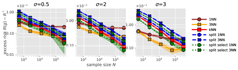
Figure 1: Summary of excess risks from the mixture of two Gaussians experiments.

4 Experiments

The goal of experiments in this section is twofold. First, we present simulated convergence rates of the $(M,k)$-NN rules for small $k$, say $k\in\{1,3\}$, are polynomial as predicted by theory with synthetic dataset. Second, we demonstrate that their practical performance is competitive against that of the standard $k$-NN rules with real-world datasets, while generally reducing both validation complexity for model selection and test complexity. In both experiments, we also show the performance of the $(M,\frac{M}{2},k)$-NN rules to examine the effect of the distance-selective aggregation.

Computing resources  For each experiment, we used a single machine with one of the following CPUs: (1) Intel(R) Core(TM) i7-9750H CPU 2.60GHz with 12 (logical) cores or (2) Intel(R) Xeon(R) CPU E5-2680 v4 @ 2.40GHz with 28 (logical) cores.

Implementation  All implementations were based on Python 3.8 and we used the NN search algorithms implemented in scikit-learn package (Pedregosa et al., 2011) ver. 0.24.1 and utilized the multiprocessors using the python standard package multiprocessing. The code can be found at https://github.com/jongharyu/split-knn-rules.

Table 1: Summary of experiments with benchmark datasets. YearPredictionMSD in the last row is a regression dataset. Recall that $(M,1)$-NN is a shorthand for the $M$-split 1-NN rules. The values in the parentheses correspond to the $(M,\frac{M}{2},1)$-NN rules. The best values are highlighted in bold.

Dataset Error (% for classification) Test time (s) Valid. time (s) 1-NN $k$-NN ($M$,1)-NN 1-NN $k$-NN ($M$,1)-NN $k$-NN ($M$,1)-NN GISETTE (Guyon et al., 2004) 7.26 $\pm 1.65$ 4.54 $\pm 0.93$ 5.11 $\pm 1.01$ (4.86 $\pm 0.86$) 6.13 5.75 6.79 (6.18) 52 262 (270)     w/ brute-force - - - 0.30 0.26 1.20 (2.06) 38 200 (207) HTRU2 (Lyon et al., 2016) 2.91 $\pm 0.40$ 2.18 $\pm 0.44$ 2.08 $\pm 0.28$ (2.28 $\pm 0.37$) 0.18 0.18 0.04 (0.04) 18 8 (10) Credit (Dua & Graff, 2019) 26.73 $\pm 0.99$ 18.68 $\pm 1.01$ 18.65 $\pm 1.05$ (18.93 $\pm 0.95$) 0.85 1.2 0.2 (0.2) 122 25 (29) MiniBooNE (Dua & Graff, 2019) 13.72 $\pm 1.57$ 10.63 $\pm 0.76$ 10.69 $\pm 0.86$ (10.62 $\pm 0.64$) 1.68 2.42 0.98 (0.94) 264 88 (92) SUSY (Baldi et al., 2014) 28.27 $\pm 1.50$ 20.32 $\pm 1.04$ 20.55 $\pm 1.35$ (20.52 $\pm 1.31$) 32 35 14 (13) 3041 1338 (1362) BNG(letter,1000,1) (Vanschoren et al., 2013) 46.13 $\pm 1.18$ 40.88 $\pm 1.12$ 41.53 $\pm 1.04$ (40.72 $\pm 0.78$) 379 350 17 (14) 2868 619 (959) YearPredictionMSD (Dua & Graff, 2019) 7.22 $\pm 0.34$ 6.72 $\pm 0.25$ 6.79 $\pm 0.22$ (6.75 $\pm 0.27$) 33 31 40 (34) 1616 431 (412)     w/ brute-force - - - 15 18 3.5 (3.6) 1529 300 (336)

4.1 Simulated Dataset

We first evaluated the performance of the proposed classifier with a synthetic data following Qiao et al. (2019). We consider a mixture of two isotropic Gaussians of equal weight $\frac{1}{2}\mathcal{N}(\mathbf{0},I_{d})+\frac{1}{2}\mathcal{N}(\mathbf{1},\sigma^{2}I_{d})$, where $\mathbf{1}\mathrel{\mathop{\mathchar 58\relax missing}}=[1,\ldots,1]^{T}\in\mathbb{R}^{d}$ and $I_{d}\in\mathbb{R}^{d\times d}$ denotes the identity matrix. With $d=5$, we tested 3 different values of $\sigma\in\{0.5,2,3\}$ with 5 different sample sizes $N\in\{500,2500,12500,62500,312500\}$. We evaluated the $(M,k)$-NN rule and $(M,\frac{M}{2},k)$-NN rule for $k\in\{1,3\}$ with $M=10N^{2\alpha_{\mathrm{H}}/(2\alpha_{\mathrm{H}}+d)}=10N^{2/7}$ based on $\alpha_{\mathrm{H}}=1$ and $d=5$. For comparison, we also ran the standard $k$-NN algorithm with $k\in\{1,3,10N^{2/7}\}$. We repeated experiments with 10 different random seeds and reported the averages and standard deviations.

The excess risks are plotted in Figure 1. We note that the $(M,1)$-NN classifier performs similarly to the baseline $k$-NN classifier across different values of $\sigma$, and the performance can be improved by the $(M,\frac{M}{2},1)$-NN classifier. This implies that discarding possibly noisy information in the aggregation could actually improve the performance of the ensemble classifier. Note also that the convergence of the excess risks of the standard $M$-NN classifier and the $(M,\{1,3\})$-NN classifiers is polynomial (indicated by the straight lines), as predicted by theory.

4.2 Real-world Datasets

We evaluated the proposed rules with publicly available benchmark datasets from the UCI machine learning repository (Dua & Graff, 2019) and the OpenML repository (Vanschoren et al., 2013), which were also used in (Xue & Kpotufe, 2018) and (Qiao et al., 2019); see Table C.1 in Appendix for size, feature dimensions, and the number of classes of each dataset. All data were standardized to have zero mean and unit variances.

We tested four algorithms. The first two algorithms are (1) the standard 1-NN rule and (2) the standard $k$-NN rule with 10-fold cross-validation (CV) over an exponential grid $k\in\mathcal{K}\mathrel{\mathop{\mathchar 58\relax missing}}=\{2^{l}-1\mathchoice{\colon}{\colon}{\mathchar 58\relax\mspace{1.0mu}}{\mathchar 58\relax}2\leq l\leq\log_{2}(\min\{2^{10},1+N_{\mathsf{train}}/25\})\}$, where $N_{\mathsf{train}}$ denotes the size of training data. The rest are (3) the $(M,1)$-NN rule and (4) the $(M,\frac{M}{2},1)$-NN rule both with 10-fold CV over $M\in\mathcal{K}$. We repeated with 10 different random (0.95,0.05) train-test splits and evaluated first $\min\{N_{\mathsf{test}},1000\}$ points from the test data to reduce the simulation time. Table 1 summarizes the test errors, test times, and validation times. The optimal $(M,1)$-NN rules consistently performed as well as the optimal standard $k$-NN rules, even running faster than the standard 1-NN rules in the test phase. We remark that the optimally tuned $(M,\frac{M}{2},1)$-NN rules (i.e., with the distance-selective aggregation) performed almost identical to the $(M,1)$-NN rules, except slight error improvements observed in high-dimensional datasets $\{\text{GISETTE, YearPredictionMSD}\}$. We additionally include Figure C.2 in Appendix which summarizes the validation error profiles from the 10-fold CV procedures.

5 Concluding Remarks

In this paper, we established the near statistical optimality of the $(M,k)$-NN rules when $k$ is fixed, which makes the sample-splitting-based NN rules more appealing for practical scenarios with large-scale data. We also removed the logarithmic factors by the distance-selective aggregation and exhibited some level of performance boost in experimental results; it is an open question whether the logarithmic factor is fundamental for the vanilla $(M,k)$-NN rules or can be removed by a tighter analysis. As supported by both theoretical guarantees and empirical supports, we believe that the $(M,k)$-NN rules, especially for $k=1$, can be widely deployed in practical systems and deserve further study including an optimally weighted version of the classifier as studied in (Duan et al., 2020). It would be also interesting if the current divide-and-conquer framework can be modified to be universally consistent for any general metric space, whenever such a consistent rule exists (Hanneke et al., 2020; Györfi & Weiss, 2021).

Overview of Appendix

In Appendix, we discuss other related work (Appendix A), prove the technical statements (Appendix B), and present some extra information on experiments (Appendix C).

Appendix A Other Related Work

The asymptotic-Bayes consistency and convergence rates of the $k$-NN classifier have been studied extensively in the last century (Fix & Hodges, 1951; Cover & Hart, 1967; Cover, 1968a, b; Wagner, 1971; Fritz, 1975; Gyorfi, 1981; Devroye et al., 1994; Kulkarni & Posner, 1995). More recent theoretical breakthroughs include a strongly consistent margin regularized 1-NN classifier (Kontorovich & Weiss, 2015), a universally consistent sample-compression based $1$-NN classifier over a general metric space (Kontorovich et al., 2017; Hanneke et al., 2020; Györfi & Weiss, 2021), nonasymptotic analysis over Euclidean space (Gadat et al., 2016) and over a doubling space (Dasgupta & Kpotufe, 2014), optimal weighted schemes (Samworth, 2012), stability (Sun et al., 2016), robustness against adversarial attacks (Wang et al., 2018; Bhattacharjee & Chaudhuri, 2020), and optimal classification with a query-dependent $k$ (Balsubramani et al., 2019). For NN-based regression (Cover, 1968a, b; Dasgupta & Kpotufe, 2014, 2019), we mostly extend the analysis techniques of (Xue & Kpotufe, 2018; Dasgupta & Kpotufe, 2019); we refer the interested reader to a recent survey of Chen et al. (2018) for more refined analyses. For a more comprehensive treatment on the $k$-NN based procedures, see (Devroye et al., 1996; Biau & Devroye, 2015) and references therein.

The most closely related work is (Qiao et al., 2019) as mentioned above. In a similar spirit, Duan et al. (2020) analyzed a distributed version of the optimally weighted NN classifier of Samworth (2012). More recently, Liu et al. (2021) studied a distributed version of an adaptive NN classification rule of Balsubramani et al. (2019).

The idea of an ensemble predictor for enhancing statistical power of a base classifier has been long known and extensively studied; see, e.g., (Hastie et al., 2009) for an overview. Among many ensemble techniques, bagging (Breiman, 1996) and pasting (Breiman, 1999) are closely related to this work. The goal of bagging is, however, mostly to improve accuracy by reducing variance when the sample size is small and the bootstrapping step is computationally demanding in general; see (Hall & Samworth, 2005; Biau et al., 2010) for the properties of bagged 1-NN rules. The motivation and idea of pasting is similar to the split NN rules, but pasting iteratively evolves an ensemble classifier based on an estimated prediction error based on random subsampling rather than splitting samples. The split NN rules analyzed in this paper are non-iterative and NN-based-rules-specific, and assume essentially no additional processing step beyond splitting and averaging.

Beyond ensemble methods, there are other attempts to make NN based rules scalable based on quantization (Kontorovich et al., 2017; Gottlieb et al., 2018; Kpotufe & Verma, 2017; Xue & Kpotufe, 2018; Hanneke et al., 2020) or regularization (Kontorovich & Weiss, 2015), where the common theme there is to carefully select subsample and/or preprocess the labels. We remark, however, that they typically involve onerous and rather complex preprocessing steps, which may not be suitable for large-scale data. Approximate NN (ANN) search algorithms (Indyk & Motwani, 1998; Slaney & Casey, 2008; Har-Peled et al., 2012) are yet another practical solution to reduce the query complexity, but ANN-search-based rules such as (Alabduljalil et al., 2013; Anastasiu & Karypis, 2019) hardly have any statistical guarantee (Dasgupta & Kpotufe, 2019) with few exception (Gottlieb et al., 2014; Efremenko et al., 2020). Gottlieb et al. (2014) proposed an ANN-based classifier for general doubling spaces with generalization bounds. More recently, Efremenko et al. (2020) proposed a locality sensitive hashing (Datar et al., 2004) based classifier with Bayes consistency but a strictly suboptimal rate guarantee in $\mathbb{R}^{d}$. In contrast, this paper focuses on exact-NN-search based algorithms.

We conclude with remarks on a seeming connection between the proposed distance-selective aggregation and the $k$-NN based outlier detection methods. Ramaswamy et al. (2000) and Angiulli & Pizzuti (2002) proposed to use the $k$-NN distance, or some basic statistics such as mean or median of the $k$-NN distances to a query point, as an outlier score; a recent paper (Gu et al., 2019) analyzed these schemes. In view of this line of work, the split-and-select NN rules can be understood as a selective ensemble of inliers based on the $k$-NN distances. It would be an interesting direction to investigate a NN-based outlier detection method for large-scale dataset, extending the idea of the distance-selective aggregation.

Appendix B Deferred Proofs

In this section, we provide the full proofs of the statements in the main text. For both regression and classification problems, the key idea in our analysis of the $(M,k)$-NN rules is to consider the $(M,L,k)$-NN rules (3.2) and (3.2) as a proof device. It relies on the observations that (1) the $(M,k)$-NN rules can be closely approximated to the $(M,\lceil\kappa M\rceil,k)$-NN rules with $\kappa\approx 1$, and (2) $(M,\lceil\kappa M\rceil,k)$-NN rules attain minimax optimality for any fixed $k$ and fixed $\kappa\in(0,1)$, as long as $M$ is chosen properly.

This section is organized as follows. In Appendix B.1, we state and prove a key technical lemma for analyzing the distributed NN rules. As the regression rules are easier to analyze, we prove Theorem 2.1 in Appendix B.2. The proof of Theorem 2.2 is presented in Appendix B.3, including an additional statement on Bayes consistency.

B.1 A Key Technical Lemma

We first restate a simple yet important observation on the $k$-nearest-neighbors by Chaudhuri & Dasgupta (2014) that the $k$-nearest neighbors of $x$ lies in a ball of probability mass of $O(\frac{k}{n})$ centered at $x$, with high probability. We define the probability radius of mass $p$ centered at $x\in\mathcal{X}$ as the minimum possible radius of a closed ball containing probability mass at least $p$, that is,

$$r_{p}(x)\mathrel{\mathop{\mathchar 58\relax missing}}=\inf\{r>0\mathchoice{\colon}{\colon}{\mathchar 58\relax\mspace{1.0mu}}{\mathchar 58\relax}\mu(B(x,r))\geq p\}.$$

Lemma B.1 (Chaudhuri & Dasgupta, 2014, Lemma 8).

Pick any $x\in\mathcal{X}$, $0\leq p\leq 1$, $0\leq\xi\leq 1$, and any positive integers $n$ and $k$ such that $k\leq\xi np$. If $X_{1},\ldots,X_{n}$ are drawn i.i.d. from $\mu$, then

$$\operatorname{\mathsf{P}}(r_{k+1}(x;X_{1\mathchar 58\relax n})>r_{p}(x)) \leq e^{-np(1-\xi)^{2}/2}\leq e^{-k(1-\xi)^{2}/(2\xi)}.$$

We now state an analogous version of the above lemma for our analysis of the $(M,k)$-NN rules. The following lemma quantifies that, with high probability (exponentially in $M$) over the split instances $\mathcal{P}_{X}$, the the $k$-nearest neighbors of $x$ from the selected data splits based on the $(k+1)$-th-NN distances will likely lie within a small probability ball of mass $O(\frac{kM}{N})$ around the query point.

Lemma B.2.

Pick any positive integer $k\geq 1$ and $\tau\in(0,1]$, and set $L=\lceil(1-\tau)^{2}M\rceil$. If the data splits ${\mathbf{X}}_{1},\ldots,{\mathbf{X}}_{M}$ are independent, we have

$$\mathsf{P}\Bigl{(}\max_{j\in[L]}r_{k+1}(x;{\mathbf{X}}_{m_{j}})>r_{p}(x)\Bigr{)} \leq e^{-\frac{(1-\tau)\tau^{2}}{2}M}$$

for $n\geq k+\ln\frac{1}{\tau}+\sqrt{2k\ln\frac{1}{\tau}+(\ln\frac{1}{\tau})^{2}}$ and $p=\frac{1}{n}(k+\ln\frac{1}{\tau}+\sqrt{2k\ln\frac{1}{\tau}+(\ln\frac{1}{\tau})^{2}})\in(0,1]$.

Proof.

Define

$$\xi=\frac{k}{k+\ln\frac{1}{\tau}+\sqrt{2k\ln\frac{1}{\tau}+(\ln\frac{1}{\tau})^{2}}}$$

so that we can write $p=\frac{k}{\xi n}=\frac{kM}{\xi N}$. Note that $\xi\in(0,1]$ for any $k\geq 1$ and $\tau\in(0,1]$.

For each data split indexed by $m\in[M]$, we define a bad event

$$E_{m}=\{r_{k+1}(x;{\mathbf{X}}_{m})>r_{p}(x)\}.$$

Observe that $E_{m}$ occurs if any only if the closed ball of probability mass $p$ contains less than $k$ points from ${\mathbf{X}}_{m}$. By Lemma B.1, the probability of the bad event $E_{m}$ is upper bounded by $e^{-k(1-\xi)^{2}/(2\xi)}$, which is equal to $\tau$ by the choice of $\xi$. Now, since the data splits are independent, $(1(E_{m}))_{m=1}^{M}$ is a sequence of independent Bernoulli random variables with parameter $\mathsf{P}(E_{1})\leq\tau$. Hence, we have

$$\mathsf{P}\Bigl{(}\max_{j\in[L]}r_{k+1}(x;{\mathbf{X}}_{m_{j}})>r_{p}(x)\Bigr{)} \leq\mathsf{P}\Bigl{(}\sum_{m=1}^{M}1(E_{m})>M-L\Bigr{)}$$

$$\leq\mathsf{P}(B_{M,1-\tau}<(1-\tau)^{2}M),$$

where $B_{M,\tau}\sim\mathrm{Binom}(M,\tau)$ denotes a binomial random variable with parameters $M$ and $\tau$. Another application of the multiplicative Chernoff bound to the right-hand side concludes the desired bound. ∎

B.2 Regression: Proof of Theorem 2.1

B.2.1 Proof of Theorem 2.1(a)

This analysis extends the proof of (Dasgupta & Kpotufe, 2019, Theorem 1.3). Let $\mathcal{P}_{X}\mathrel{\mathop{\mathchar 58\relax missing}}=\{{\mathbf{X}}_{m}\}_{m=1}^{M}$ denote the set of splits of ${\mathbf{X}}$. We let $V\mathrel{\mathop{\mathchar 58\relax missing}}=\sup_{x\in\mathcal{X}}v(x)<\infty$ and $H\mathrel{\mathop{\mathchar 58\relax missing}}=\sup_{x\in\mathcal{X}}\mathchoice{\mspace{1.0mu}|\mspace{1.0mu}}{|}{|}{|}\eta(x)\mathchoice{\mspace{1.0mu}|\mspace{1.0mu}}{|}{|}{|}<\infty$. Since the support of $\mu$ is bounded, we let $R\mathrel{\mathop{\mathchar 58\relax missing}}=\operatorname*{diam}(\textnormal{supp}(\mu))<\infty$.

Step 1. Error decomposition

Recall that we wish to bound

$$\mathbb{E}_{\mathcal{P}}\|\tilde{\eta}_{M}^{(k)}-\eta\|_{2} =\mathbb{E}_{\mathcal{P}}\sqrt{\mathbb{E}_{X}[(\tilde{\eta}^{(k)}(X;\mathcal{P})-\eta(X))^{2}]}$$

$$\leq\sqrt{\mathbb{E}_{\mathcal{P}}\mathbb{E}_{X}[(\tilde{\eta}^{(k)}(X;\mathcal{P})-\eta(X))^{2}]}.$$

Here, the inequality follows by Jensen’s inequality. We will consider the $(M,L,k)$-NN regression rule with $L=\lceil(1-\tau)^{2}M\rceil$ as a proof device, where $\tau$ is to be determined at the end of the proof. Pick any $x\in\mathcal{X}$. We denote the conditional expectation of the $(M,L,k)$-NN regression estimate $\breve{\eta}_{L}^{(k)}(x;\mathcal{P})$ by

$$\overline{\eta}_{L}^{(k)}(x;\mathcal{P}_{X}) \mathrel{\mathop{\mathchar 58\relax missing}}=\mathbb{E}_{\mathbf{Y}\mathchoice{\mspace{1.0mu}|\mspace{1.0mu}}{|}{|}{|}\mathcal{P}_{X}}[\breve{\eta}_{L}^{(k)}(x;\mathcal{P})]=\frac{1}{kL}\sum_{j=1}^{L}\sum_{i=1}^{k}\eta(X_{(i)}(x;{\mathbf{X}}_{m_{j}})),$$

where the expectation is over $Y$-values $\mathbf{Y}$ given the data splits $\mathcal{P}_{X}$. Note that with $L=M$, $\overline{\eta}_{M}^{(k)}(x;\mathcal{P}_{X})$ becomes the conditional expectation of the $(M,k)$-NN regression estimate $\tilde{\eta}^{(k)}(x;\mathcal{P})$. We decompose the squared error $(\tilde{\eta}^{(k)}(x;\mathcal{P})-\eta(x))^{2}$ as

$$(\tilde{\eta}^{(k)}(x;\mathcal{P})-\eta(x))^{2}$$

$$=\Bigl{(}\tilde{\eta}^{(k)}(x;\mathcal{P})-\overline{\eta}_{M}^{(k)}(x;\mathcal{P}_{X})+\overline{\eta}_{M}^{(k)}(x;\mathcal{P}_{X})-\overline{\eta}_{L}^{(k)}(x;\mathcal{P}_{X})+\overline{\eta}_{L}^{(k)}(x;\mathcal{P}_{X})-\eta(x)\Bigr{)}^{2}$$

$$\leq 3\Bigl{\{}(\tilde{\eta}^{(k)}(x;\mathcal{P})-\overline{\eta}_{M}^{(k)}(x;\mathcal{P}_{X}))^{2}+(\overline{\eta}_{M}^{(k)}(x;\mathcal{P}_{X})-\overline{\eta}_{L}^{(k)}(x;\mathcal{P}_{X}))^{2}+(\overline{\eta}_{L}^{(k)}(x;\mathcal{P}_{X})-\eta(x))^{2}\Bigr{\}},$$

where we use the inequality $(a+b+c)^{2}\leq 3(a^{2}+b^{2}+c^{2})$. Taking expectation over the $Y$ values given the data splits $\mathcal{P}_{X}$, we have

$$\mathbb{E}_{\mathbf{Y}\mathchoice{\mspace{1.0mu}|\mspace{1.0mu}}{|}{|}{|}\mathcal{P}_{X}}[(\tilde{\eta}^{(k)}(x;\mathcal{P})-\eta(x))^{2}] \leq 3\Bigl{\{}\underbrace{\mathop{\rm Var}\nolimits_{\mathbf{Y}\mathchoice{\mspace{1.0mu}|\mspace{1.0mu}}{|}{|}{|}\mathcal{P}_{X}}(\tilde{\eta}^{(k)}(x;\mathcal{P}))}_{(A)}$$ (B.1)

$$\qquad+\underbrace{\mathbb{E}_{\mathbf{Y}\mathchoice{\mspace{1.0mu}|\mspace{1.0mu}}{|}{|}{|}\mathcal{P}_{X}}[(\overline{\eta}_{M}^{(k)}(x;\mathcal{P}_{X})-\overline{\eta}_{L}^{(k)}(x;\mathcal{P}_{X}))^{2}]}_{(B)}$$

$$\qquad+\underbrace{(\overline{\eta}_{L}^{(k)}(x;\mathcal{P}_{X})-\eta(x))^{2}}_{(C)}\Bigr{\}}.$$

We now bound the three terms separately in the next steps.

Step 2(A). Variance term

Consider

$$\mathop{\rm Var}\nolimits_{\mathbf{Y}\mathchoice{\mspace{1.0mu}|\mspace{1.0mu}}{|}{|}{|}\mathcal{P}_{X}}(\tilde{\eta}^{(k)}(x;\mathcal{P})) =\mathbb{E}_{\mathbf{Y}\mathchoice{\mspace{1.0mu}|\mspace{1.0mu}}{|}{|}{|}\mathcal{P}_{X}}[(\tilde{\eta}^{(k)}(x;\mathcal{P})-\overline{\eta}_{M}^{(k)}(x;\mathcal{P}))^{2}]$$

$$=\mathbb{E}_{\mathbf{Y}\mathchoice{\mspace{1.0mu}|\mspace{1.0mu}}{|}{|}{|}\mathcal{P}_{X}}\Bigl{[}\Bigl{(}\frac{1}{kM}\sum_{i=1}^{k}\sum_{m=1}^{M}(Y_{(i)}(x;\mathcal{D}_{m})-\mathbb{E}[Y_{(i)}(x;\mathcal{D}_{m})\mathchoice{\mspace{1.0mu}|\mspace{1.0mu}}{|}{|}{|}\mathcal{P}_{X}])\Bigr{)}^{2}\Bigr{]}$$

$$\stackrel{{\scriptstyle\mathchoice{\hbox to0.0pt{\hss$\displaystyle{(a)}$\hss}}{\hbox to0.0pt{\hss$\textstyle{(a)}$\hss}}{\hbox to0.0pt{\hss$\scriptstyle{(a)}$\hss}}{\hbox to0.0pt{\hss$\scriptscriptstyle{(a)}$\hss}}}}{{=}}\frac{1}{(kM)^{2}}\sum_{i=1}^{k}\sum_{m=1}^{M}\mathop{\rm Var}\nolimits_{\mathbf{Y}\mathchoice{\mspace{1.0mu}|\mspace{1.0mu}}{|}{|}{|}\mathcal{P}_{X}}(Y_{(i)}(x;\mathcal{D}_{m}))$$

$$=\frac{1}{(kM)^{2}}\sum_{i=1}^{k}\sum_{m=1}^{M}v(X_{(i)}(x;\mathbf{X}_{m}))\stackrel{{\scriptstyle\mathchoice{\hbox to0.0pt{\hss$\displaystyle{(b)}$\hss}}{\hbox to0.0pt{\hss$\textstyle{(b)}$\hss}}{\hbox to0.0pt{\hss$\scriptstyle{(b)}$\hss}}{\hbox to0.0pt{\hss$\scriptscriptstyle{(b)}$\hss}}}}{{\leq}}\frac{V}{kM}.$$ (B.2)

Here, (a) follows by the independence of $Y_{i}$’s conditioned on the splits $\mathcal{P}_{X}$ and (b) follows from the assumption $v(x)\leq V$ for all $x\in\mathcal{X}$.

Step 2(B). Approximation term

We claim that the second term $(B)$ is bounded as $O(\tau^{2})$. We have

$$\mathchoice{\mspace{1.0mu}|\mspace{1.0mu}}{|}{|}{|}\overline{\eta}_{M}^{(k)}(x;\mathcal{P})-\overline{\eta}_{L}^{(k)}(x;\mathcal{P})\mathchoice{\mspace{1.0mu}|\mspace{1.0mu}}{|}{|}{|} \leq\Bigl{(}1-\frac{L}{M}\Bigr{)}\mathchoice{\mspace{1.0mu}|\mspace{1.0mu}}{|}{|}{|}\overline{\eta}_{L}^{(k)}(x;\mathcal{P})\mathchoice{\mspace{1.0mu}|\mspace{1.0mu}}{|}{|}{|}+\Bigl{\mathchoice{\mspace{1.0mu}|\mspace{1.0mu}}{|}{|}{|}missing}\frac{1}{M}\sum_{j=L+1}^{M}\frac{1}{k}\sum_{i=1}^{k}\eta(X_{(i)}(x;{\mathbf{X}}_{m_{j}}))\Bigr{\mathchoice{\mspace{1.0mu}|\mspace{1.0mu}}{|}{|}{|}missing}$$

$$\stackrel{{\scriptstyle\mathchoice{\hbox to0.0pt{\hss$\displaystyle{(a)}$\hss}}{\hbox to0.0pt{\hss$\textstyle{(a)}$\hss}}{\hbox to0.0pt{\hss$\scriptstyle{(a)}$\hss}}{\hbox to0.0pt{\hss$\scriptscriptstyle{(a)}$\hss}}}}{{\leq}}\Bigl{(}1-\frac{L}{M}\Bigr{)}H+\frac{M-L}{M}H$$

$$=2H\Bigl{(}1-\frac{L}{M}\Bigr{)}$$

$$\stackrel{{\scriptstyle\mathchoice{\hbox to0.0pt{\hss$\displaystyle{(b)}$\hss}}{\hbox to0.0pt{\hss$\textstyle{(b)}$\hss}}{\hbox to0.0pt{\hss$\scriptstyle{(b)}$\hss}}{\hbox to0.0pt{\hss$\scriptscriptstyle{(b)}$\hss}}}}{{\leq}}4H\tau,$$ (B.3)

where (a) follows by the assumption $\mathchoice{\mspace{1.0mu}|\mspace{1.0mu}}{|}{|}{|}\eta(x)\mathchoice{\mspace{1.0mu}|\mspace{1.0mu}}{|}{|}{|}\leq H$ for all $x\in\mathcal{X}$ and (b) follows since $L=\lceil(1-\tau)^{2}M\rceil\geq(1-2\tau)M$.

Step 2(C). Bias term

It only remains to bound the term $(C)$, which is the bias of the $(M,L,k)$-NN regression estimate $\breve{\eta}_{L}^{(k)}(x;\mathcal{P})$. Since $\eta$ is $(\alpha_{\mathrm{H}},A)$-Hölder continuous, it immediately follows that

$$\mathchoice{\mspace{1.0mu}|\mspace{1.0mu}}{|}{|}{|}\overline{\eta}_{L}^{(k)}(x;\mathcal{P}_{X})-\eta(x)\mathchoice{\mspace{1.0mu}|\mspace{1.0mu}}{|}{|}{|} \leq\frac{1}{kL}\sum_{i=1}^{k}\sum_{j=1}^{L}\mathchoice{\mspace{1.0mu}|\mspace{1.0mu}}{|}{|}{|}\eta(X_{(i)}(x;{\mathbf{X}}_{m_{j}}))-\eta(x)\mathchoice{\mspace{1.0mu}|\mspace{1.0mu}}{|}{|}{|}$$

$$\leq A\max_{j\in[L]}r_{k+1}^{\alpha_{\mathrm{H}}}(x;{\mathbf{X}}_{m_{j}}).$$

Now, for any $p\in(0,1)$, we observe that by the homogeneity of $\mu$, we have

$$C_{d}\Bigl{(}\frac{r_{p}(x)}{2}\Bigr{)}^{d}\leq\mu\Bigl{(}B^{o}\Bigl{(}x,\frac{r_{p}(x)}{2}\Bigr{)}\Bigr{)}<p,$$

which implies that $r_{p}(x)<2(\frac{p}{C_{d}})^{1/d}$. Now, if we set $p=\frac{1}{n}(k+\ln\frac{1}{\tau}+\sqrt{2k\ln\frac{1}{\tau}+(\ln\frac{1}{\tau})^{2}})$, then by Lemma B.2 and the boundedness of the support, i.e., $\operatorname*{diam}(\textnormal{supp}(\mu))\leq R$, we have

$$\mathbb{E}_{\mathcal{P}_{X}}[(\overline{\eta}_{L}^{(k)}(x;\mathcal{P}_{X})-\eta(x))^{2}] \leq A^{2}\mathbb{E}_{\mathcal{P}_{X}}\Bigl{[}\max_{j\in[L]}r_{k+1}^{2\alpha_{\mathrm{H}}}(x;{\mathbf{X}}_{m_{j}})\Bigr{]}$$

$$\leq A^{2}\Bigl{\{}r_{p}^{2\alpha_{\mathrm{H}}}(x)+R^{2\alpha_{\mathrm{H}}}\operatorname{\mathsf{P}}\Bigl{(}\max_{j\in[L]}r_{k+1}(x;{\mathbf{X}}_{m_{j}})>r_{p}(x)\Bigr{)}\Bigr{\}}$$

$$\leq A^{2}\Bigl{(}2^{2\alpha_{\mathrm{H}}}\Bigl{(}\frac{p}{C_{d}}\Bigr{)}^{\frac{2\alpha_{\mathrm{H}}}{d}}+R^{2\alpha_{\mathrm{H}}}e^{-\frac{(1-\tau)\tau^{2}}{2}M}\Bigr{)}.$$ (B.4)

Step 3.

Plugging in (B.2), (B.3), and (B.4) to the error decomposition (B.1) leads to

$$\mathbb{E}[(\tilde{\eta}^{(k)}(x;\mathcal{P})-\eta(x))^{2}] \leq 3\Bigl{\{}\frac{V}{kM}+16H^{2}\tau^{2}+A^{2}2^{2\alpha_{\mathrm{H}}}\Bigl{(}\frac{p}{C_{d}}\Bigr{)}^{\frac{2\alpha_{\mathrm{H}}}{d}}+A^{2}R^{2\alpha_{\mathrm{H}}}e^{-\frac{(1-\tau)\tau^{2}}{2}M}\Bigr{\}}.$$

If we set $\tau=\sqrt{(\ln M)^{1.01}/M}$, then we obtain the desired bound since $p=O(\frac{1}{n}(k+\ln\frac{1}{\tau}))=O(\frac{M}{N}\ln M)$ and $e^{-\frac{(1-\tau)\tau^{2}}{2}M}=e^{-\frac{1}{2}(\ln M)^{1.01}(1-\tau)}$ decays faster than any polynomial rate.∎

B.2.2 Proof of Theorem 2.1(b)

This analysis adopts the proof technique of (Xue & Kpotufe, 2018, Proposition 1) and will invoke the following lemma therein.

Lemma B.3 (Xue & Kpotufe, 2018, Lemma 1).

Assume that $\mu$ is a $(C_{d},d)$-homogeneous measure and the collection of all closed balls in $\mathcal{X}$ has finite VC dimension $\mathcal{V}$. Then, with probability at least $1-\tau$ over the sample ${\mathbf{X}}$ of size $n$, for any $k\in[n]$, we have

$$\sup_{x\in\mathcal{X}}r_{k}(x;{\mathbf{X}})\leq\Bigl{(}\frac{3}{C_{d}n}\Bigl{(}k\vee\Bigl{(}\mathcal{V}\log 2n+\log\frac{8}{\tau}\Bigr{)}\Bigr{)}\Bigr{)}^{\frac{1}{d}}.$$

Step 1. Approximate with $(M,L,k)$-NN estimator

We consider the $(M,L,k)$-NN regression estimate $\breve{\eta}_{L}^{(k)}(x;\mathcal{P})$ with $L=\lceil(1-\tau)^{2}M\rceil$, where $\tau$ is to be determined. Similar to the proof of Theorem 2.1(a), we can decompose and upper-bound the error of $\tilde{\eta}_{M}^{(k)}$ as

$$\|\tilde{\eta}_{M}^{(k)}-\eta\|_{\infty} \leq\|\tilde{\eta}_{M}^{(k)}-\breve{\eta}_{L}^{(k)}\|_{\infty}+\|\breve{\eta}_{L}^{(k)}-\eta\|_{\infty}\leq 4H\tau+\|\breve{\eta}_{L}^{(k)}-\eta\|_{\infty}.$$ (B.5)

That is, with the approximation error $4H\tau$, it suffices to analyze the $(M,L,k)$-NN estimator $\breve{\eta}_{L}^{(k)}(x;\mathcal{P})$.

Step 2. Analyze $(M,L,k)$-NN estimator

To bound the sup-norm $\|\breve{\eta}_{L}^{(k)}-\eta\|_{\infty}=\sup_{x\in\mathcal{X}}\mathchoice{\mspace{1.0mu}|\mspace{1.0mu}}{|}{|}{|}\breve{\eta}_{L}^{(k)}(x;\mathcal{P})-\eta(x)\mathchoice{\mspace{1.0mu}|\mspace{1.0mu}}{|}{|}{|}$, we consider the following bias-variance decomposition

$$\mathchoice{\mspace{1.0mu}|\mspace{1.0mu}}{|}{|}{|}\breve{\eta}_{L}^{(k)}(x;\mathcal{P})-\eta(x)\mathchoice{\mspace{1.0mu}|\mspace{1.0mu}}{|}{|}{|} \leq\underbrace{\mathchoice{\mspace{1.0mu}|\mspace{1.0mu}}{|}{|}{|}\overline{\eta}_{L}^{(k)}(x;\mathcal{P}_{X})-\eta(x)\mathchoice{\mspace{1.0mu}|\mspace{1.0mu}}{|}{|}{|}missing}_{\text{bias}}+\underbrace{\mathchoice{\mspace{1.0mu}|\mspace{1.0mu}}{|}{|}{|}\breve{\eta}_{L}^{(k)}(x;\mathcal{P})-\overline{\eta}_{L}^{(k)}(x;\mathcal{P}_{X})\mathchoice{\mspace{1.0mu}|\mspace{1.0mu}}{|}{|}{|}missing}_{\text{variance}},$$

where we define the conditional expectation $\overline{\eta}_{L}^{(k)}(x;\mathcal{P}_{X})\mathrel{\mathop{\mathchar 58\relax missing}}=\mathbb{E}[\breve{\eta}_{L}^{(k)}(x;\mathcal{P})\mathchoice{\mspace{1.0mu}|\mspace{1.0mu}}{|}{|}{|}\mathcal{P}_{X}]$ as in the proof of Theorem 2.1(a).

Step 2(a). Bias bound

The following lemma, which is a variant of Lemma B.2, can be readily shown by invoking Lemma B.3 with $n\leftarrow N/M$ and following the same line of the proof of Lemma B.2.

Lemma B.4.

Assume that $\mu$ is a $(C_{d},d)$-homogeneous measure and the collection of all closed balls in $\mathcal{X}$ has finite VC dimension $\mathcal{V}$. Pick any $\delta\in(0,1)$. If the data splits $\mathcal{P}_{X}=\{{\mathbf{X}}_{m}\}_{m=1}^{M}$ are independent and of equal size $N/M$, for $L\mathrel{\mathop{\mathchar 58\relax missing}}=\lceil(1-\tau)^{2}M\rceil$, we have

$$\mathsf{P}\Bigl{(}\max_{j\in[L]}r_{k}(x;{\mathbf{X}}_{m_{j}})>\Bigl{(}\frac{3M}{C_{d}N}\Bigl{(}k\vee\Bigl{(}\mathcal{V}\log\frac{2N}{M}+\log\frac{8}{\tau}\Bigr{)}\Bigr{)}\Bigr{)}^{\frac{1}{d}}\Bigr{)}\leq e^{-\frac{(1-\tau)\tau^{2}}{2}M}.$$

For $M\geq 16\log\frac{1}{\delta}$, we define $\tau=\sqrt{\frac{4}{M}\log\frac{1}{\delta}}\leq\frac{1}{2}$ so that $\delta=e^{-\frac{\tau^{2}M}{4}}\geq e^{-\frac{(1-\tau)\tau^{2}M}{2}}$. Then, Lemma B.4 and the Hölder continuity of $\eta$ imply that with probability at least $1-\delta$ over the data splits $\mathcal{P}_{X}$, we have

$$\sup_{x\in\mathcal{X}}\mathchoice{\mspace{1.0mu}|\mspace{1.0mu}}{|}{|}{|}\overline{\eta}_{L}^{(k)}(x;\mathcal{P}_{X})-\eta(x)\mathchoice{\mspace{1.0mu}|\mspace{1.0mu}}{|}{|}{|} \leq A\sup_{x\in\mathcal{X}}\max_{j\in[L]}r_{k}^{\alpha_{\mathrm{H}}}(x;{\mathbf{X}}_{m_{j}})$$

$$\leq A\Bigl{(}\frac{3M}{C_{d}N}\Bigl{(}k\vee\Bigl{(}\mathcal{V}\log\frac{2N}{M}+\frac{1}{2}\log\frac{16M}{\log\frac{1}{\delta}}\Bigr{)}\Bigr{)}\Bigr{)}^{\frac{\alpha_{\mathrm{H}}}{d}}.$$ (B.6)

Step 2(b). Variance bound

For any fixed $x\in\mathcal{X}$ and split instances $\mathcal{P}_{X}=\{{\mathbf{X}}_{m}\}_{m=1}^{M}$, Hoeffding’s inequality guarantees that with probability at least $1-\delta_{o}$ over the labels $\{\mathbf{Y}_{m}\}_{m=1}^{M}$, we have

$$\mathchoice{\mspace{1.0mu}|\mspace{1.0mu}}{|}{|}{|}\breve{\eta}_{L}^{(k)}(x;\mathcal{P})-\overline{\eta}_{L}^{(k)}(x;\mathcal{P}_{X})\mathchoice{\mspace{1.0mu}|\mspace{1.0mu}}{|}{|}{|}\leq\sqrt{\frac{l_{Y}^{2}}{2kL}\log\frac{2}{\delta_{o}}}.$$ (B.7)

Now, observe that given $\mathcal{P}_{X}$, the left hand side is a function of $x$ only via its nearest neighbors from ${\mathbf{X}}$, and thus only depends on a closed ball centered at $x$. The finite VC dimensionality assumption then implies that if we vary $x\in\mathcal{X}$, there are at most $(eN/\mathcal{V})^{\mathcal{V}}$ different such inequalities (B.7). Hence, letting $\delta=\delta_{o}(eN/\mathcal{V})^{\mathcal{V}}$ and applying union bound, we have, with probability at least $1-\delta$ over $\{\mathbf{Y}_{m}\}_{m=1}^{M}$,

$$\sup_{x\in\mathcal{X}}\mathchoice{\mspace{1.0mu}|\mspace{1.0mu}}{|}{|}{|}\breve{\eta}_{L}^{(k)}(x;\mathcal{P})-\overline{\eta}_{L}^{(k)}(x;\mathcal{P}_{X})\mathchoice{\mspace{1.0mu}|\mspace{1.0mu}}{|}{|}{|}\leq\sqrt{\frac{\mathcal{V}l_{Y}^{2}}{kL}\log\frac{N}{\delta}}.$$ (B.8)

Since this inequality holds independent of $\mathcal{P}_{X}$, it also holds with probability at least $1-\delta$ over the split data $\mathcal{P}$.

Step 3.

Continuing from (B.5) and combining the bias bound (B.6) and variance bound (B.8) by union bound, we have with probability at least $1-\delta$,

$$\|\tilde{\eta}_{M}^{(k)}-\eta\|_{\infty} \leq 4H\sqrt{\frac{4}{M}\ln\frac{1}{\delta}}+A\Bigl{(}\frac{3M}{C_{d}N}\Bigl{(}k\vee\Bigl{(}\mathcal{V}\log\frac{2N}{M}+\frac{1}{2}\log\frac{16M}{\log\frac{1}{\delta}}\Bigr{)}\Bigr{)}\Bigr{)}^{\frac{\alpha_{\mathrm{H}}}{d}}$$

$$\qquad+\sqrt{\frac{\mathcal{V}l_{Y}^{2}}{kL}\log\frac{2N}{\delta}},$$

which leads to the desired bound. ∎

B.3 Classification

All theoretical guarantees on classifiers in this paper are analogous to the results for the standard $k$-NN classifier established in the seminal paper by Chaudhuri & Dasgupta (2014).

B.3.1 Definitions

We first review some technical definitions introduced in (Chaudhuri & Dasgupta, 2014). For any $x\in\mathcal{X}$ and any $0\leq p\leq 1$, define the probability radius of a ball centered at $x$ as

$$r_{p}(x)=\inf\{r\mathchoice{\colon}{\colon}{\mathchar 58\relax\mspace{1.0mu}}{\mathchar 58\relax}\mu(B(x,r))\geq p\}.$$

One can show that $\mu(B^{o}(x,r_{p}(x)))\geq p$, and $r_{p}(x)$ is the smallest radius for which this holds.

The support of the distribution $\mu$ is defined as

$$\textnormal{supp}(\mu)\mathrel{\mathop{\mathchar 58\relax missing}}=\{x\in\mathcal{X}\mathchoice{\colon}{\colon}{\mathchar 58\relax\mspace{1.0mu}}{\mathchar 58\relax}\mu(B(x,r))>0,\forall r>0\}.$$

In separable metric spaces, it can be shown that $\mu(\textnormal{supp}(\mu))=1$; see (Cover & Hart, 1967) or (Chaudhuri & Dasgupta, 2014, Lemma 24).

We define for any measurable set $A\subset\mathcal{X}$ with $\mu(A)>0$,

$$\eta(A)\mathrel{\mathop{\mathchar 58\relax missing}}=p(y=1\mathchoice{\mspace{1.0mu}|\mspace{1.0mu}}{|}{|}{|}A)=\frac{1}{\mu(A)}\int_{A}p(y=1\mathchoice{\mspace{1.0mu}|\mspace{1.0mu}}{|}{|}{|}x)\mathop{}\!\mathrm{d}\mu(x).$$

This is the conditional probability of $Y$ being 1 given a point $X$ chosen at random from the distribution $\mu$ restricted to the set $A$.

Based on the definitions above, we now define the effective interiors of the two classes, and the effective boundary. For $p\in[0,1]$ and $\Delta>0$, we define the effective interiors for each class as

$$\mathcal{X}_{p,\Delta}^{+} \mathrel{\mathop{\mathchar 58\relax missing}}=\textnormal{supp}(\mu)\cap\Bigl{\{}x\in\mathcal{X}\mathchoice{\colon}{\colon}{\mathchar 58\relax\mspace{1.0mu}}{\mathchar 58\relax}\eta(x)>\frac{1}{2}\Bigr{\}}\cap\Bigl{\{}x\in\mathcal{X}\mathchoice{\colon}{\colon}{\mathchar 58\relax\mspace{1.0mu}}{\mathchar 58\relax}\eta(B(x,r))\geq\frac{1}{2}+\Delta,\forall r\leq r_{p}(x)\Bigr{\}}$$

and

$$\mathcal{X}_{p,\Delta}^{-} \mathrel{\mathop{\mathchar 58\relax missing}}=\textnormal{supp}(\mu)\cap\Bigl{\{}x\in\mathcal{X}\mathchoice{\colon}{\colon}{\mathchar 58\relax\mspace{1.0mu}}{\mathchar 58\relax}\eta(x)<\frac{1}{2}\Bigr{\}}\cap\Bigl{\{}x\in\mathcal{X}\mathchoice{\colon}{\colon}{\mathchar 58\relax\mspace{1.0mu}}{\mathchar 58\relax}\eta(B(x,r))\leq\frac{1}{2}-\Delta,\forall r\leq r_{p}(x)\Bigr{\}}.$$

For a measurable set $A\subseteq\mathcal{X}$, we define ${\hat{Y}}(A;\mathcal{D})$ as the mean of $Y_{i}$ for points $X_{i}\in A$ given data $\mathcal{D}=({\mathbf{X}},\mathbf{Y})$. The quantity ${\hat{Y}}(A;\mathcal{D})$ is not defined if there exists no sample point $X_{i}$ in $A$. We also define an average conditional distribution $\eta(A)\mathrel{\mathop{\mathchar 58\relax missing}}=\frac{1}{\mu(A)}\int_{A}\eta\mathop{}\!\mathrm{d}\mu$ whenever $\mu(A)>0$.

Let $g(x)\mathrel{\mathop{\mathchar 58\relax missing}}=1(\eta(x)\geq 1/2)$ denote the Bayes classifier. Let ${\hat{g}}^{(k)}(x;\mathcal{D})$ denote the $k$-NN classifier based on training data $\mathcal{D}=({\mathbf{X}},\mathbf{Y})$. Note that we can equivalently write

$${\hat{g}}^{(k)}(x;\mathcal{D})=\mathds{1}\Bigl{(}{\hat{Y}}(B_{k}(x;\mathcal{D}))\geq\frac{1}{2}\Bigr{)}.$$

For the sake of simplicity, we assume that there is no distance tie in what follows, but it can be handled by a similar argument in (Chaudhuri & Dasgupta, 2014).

B.3.2 A key technical lemma

The analysis of the standard $k$-NN classifier by Chaudhuri & Dasgupta (2014) relies on their key lemma (Chaudhuri & Dasgupta, 2014, Lemma 7), which proves a sufficient condition for the $k$-NN classifier to agree with the Bayes classifier. In this section, we provide an analogous lemma for the $(M,k)$-NN classifier. The key idea is to leverage the closeness of the $(M,k)$-NN classifier to a $(M,L,k)$-NN classifier for $L\leq M$ sufficiently large. We remark that the following lemma is the only place we use the $(M,L,k)$-NN rule in the rest of our analysis.

Lemma B.5 (cf. (Chaudhuri & Dasgupta, 2014, Lemma 7)).

Pick any $x_{o}\in\mathcal{X}$, any $p\in(0,1)$, $\Delta\in(0,1/2]$, and $\tau\in(0,\frac{\Delta}{8}]$. Let $L\mathrel{\mathop{\mathchar 58\relax missing}}=\lceil(1-\tau)^{2}M\rceil$. For each $m\in[M]$, define $B_{m}\mathrel{\mathop{\mathchar 58\relax missing}}=B^{o}(x_{o},r_{k+1}(x_{o};{\mathbf{X}}_{m}))$. Then, we have

$$\mathds{1}({\tilde{g}}^{(k)}(x_{o};\mathcal{P})\neq g(x_{o})) \leq\mathds{1}(x_{o}\in\mathop{}\!\partial_{p,\Delta})$$

$$\quad+\mathds{1}\Bigl{(}\max_{j\in[L]}r_{k+1}(x_{o};{\mathbf{X}}_{m_{j}})>r_{p}(x_{o})\Bigr{)}$$

$$\quad+\mathds{1}\Bigl{(}\Bigl{\mathchoice{\mspace{1.0mu}|\mspace{1.0mu}}{|}{|}{|}missing}\frac{1}{L}\sum_{j=1}^{L}({\hat{Y}}(B_{m_{j}};\mathcal{D}_{m_{j}})-\eta(B_{m_{j}}))\Bigr{\mathchoice{\mspace{1.0mu}|\mspace{1.0mu}}{|}{|}{|}missing}\geq\frac{\Delta}{2}\Bigr{)},$$ (B.9)

where $m_{1},\ldots,m_{L}$ are the indices that correspond to the $L$-smallest values among $(r_{k+1}(x_{o};{\mathbf{X}}_{m}))_{m=1}^{M}$.

Proof.

Suppose $x_{o}\notin\mathop{}\!\partial_{p,\Delta}$. Without loss of generality, consider $x_{o}\in\mathcal{X}_{p,\Delta}^{+}$, whereupon $g(x_{o})=1$. By definition of the effective interior, $\eta(B(x_{o},r))\geq\frac{1}{2}+\Delta$ for all $r\leq r_{p}(x_{o})$.

Now, suppose

$$\max_{j\in[L]}r_{k+1}(x_{o};{\mathbf{X}}_{m_{j}})\leq r_{p}(x_{o}).$$

Then, we have, for any $j\in[L]$, that

$$\eta(B_{m_{j}})=\eta(B^{o}(x_{o},r_{k+1}(x_{o};{\mathbf{X}}_{m_{j}})))\geq\frac{1}{2}+\Delta,$$

by Lemma B.6 (stated below).

Further, if $\mathchoice{\mspace{1.0mu}|\mspace{1.0mu}}{|}{|}{|}\frac{1}{L}\sum_{j=1}^{L}({\hat{Y}}(B_{m_{j}};\mathcal{D}_{m_{j}})-\eta(B_{m_{j}}))\mathchoice{\mspace{1.0mu}|\mspace{1.0mu}}{|}{|}{|}<\frac{\Delta}{2}$, then

$$\breve{\eta}_{L}^{(k)}(x_{o};\mathcal{P})=\frac{1}{L}\sum_{j=1}^{L}{\hat{Y}}(B_{m_{j}};\mathcal{D}_{m_{j}})\geq\frac{1}{2}+\frac{\Delta}{2},$$

where we recall that $\breve{\eta}_{L}^{(k)}(\cdot;\mathcal{P})$ denotes the $(M,L,k)$-NN regressor based on the training data splits $\mathcal{P}=\{({\mathbf{X}}_{m},\mathbf{Y}_{m})\}_{m=1}^{M}$.

Finally, since $\mathchoice{\mspace{1.0mu}|\mspace{1.0mu}}{|}{|}{|}\tilde{\eta}^{(k)}(x_{o};\mathcal{P})-\breve{\eta}_{L}^{(k)}(x_{o};\mathcal{P})\mathchoice{\mspace{1.0mu}|\mspace{1.0mu}}{|}{|}{|}\leq 2(1-\frac{L}{M})<4\tau\leq\frac{\Delta}{2}$, we have $\tilde{\eta}^{(k)}(x_{o};\mathcal{P})>\frac{1}{2}$, which concludes ${\tilde{g}}^{(k)}(x_{o};\mathcal{P})=1=g(x_{o})$. ∎

Lemma B.6 (Chaudhuri & Dasgupta, 2014, Lemma 26).

Suppose that for some $x_{o}\in\textnormal{supp}(\mu)$ and $r_{o}>0$ and $q>0$, we have [$r\leq r_{o}$ $\Rightarrow$ $\eta(B(x_{o},r))\geq q$]. Then, we also have [$r\leq r_{o}$ $\Rightarrow$ $\eta(B^{o}(x_{o},r))\geq q$].

B.3.3 A general upper bound on the misclassification error

We first present a generalization of the main result in (Chaudhuri & Dasgupta, 2014), which is a general upper bound on the misclassification error rate. Theorem 2.2(a) and (b) will almost readily follow as corollaries of this theorem.

Theorem B.7 (cf. (Chaudhuri & Dasgupta, 2014, Theorem 5)).

Let $k\geq 1$ be fixed and pick any $\delta\in(0,1)$. Pick any integer $M\geq\frac{2^{14}}{15}\log\frac{2}{\delta}$, set $\Delta\mathrel{\mathop{\mathchar 58\relax missing}}=\sqrt{\frac{2^{12}}{15M}\log\frac{2}{\delta}}\in(0,\frac{1}{2}]$. Pick any integer $n\geq k+\log\frac{8}{\Delta}+\sqrt{2k\log\frac{8}{\Delta}+(\log\frac{8}{\Delta})^{2}}$ and set $p\mathrel{\mathop{\mathchar 58\relax missing}}=\frac{1}{n}(k+\log\frac{8}{\Delta}+\sqrt{2k\log\frac{8}{\Delta}+(\log\frac{8}{\Delta})^{2}})\in(0,1]$. Then, for a set of data splits $\mathcal{P}=\{\mathcal{D}_{1},\ldots,\mathcal{D}_{M}\}$, where every split $\mathcal{D}_{m}$ has $n$ data points, with probability at least $1-\delta$ over $\mathcal{P}$, we have

$$\mathsf{P}({\tilde{g}}^{(k)}(X;\mathcal{P})\neq g(X)\mathchoice{\mspace{1.0mu}|\mspace{1.0mu}}{|}{|}{|}\mathcal{P})\leq\delta+\mu(\mathop{}\!\partial_{p,\Delta}).$$

Proof.

Given $k\geq 1$, $\delta\in(0,1)$, and $\Delta\in(0,1/2]$, we set $\tau=\frac{\Delta}{8}$ and define $L=\lceil(1-\tau)^{2}M\rceil$ as stated in Lemma B.2. Pick any $x_{o}\in\mathcal{X}$. Applying Lemma B.5, we have

$$\mathds{1}({\tilde{g}}^{(k)}(x_{o};\mathcal{P})\neq g(x_{o})) \leq\mathds{1}(x_{o}\in\mathop{}\!\partial_{p,\Delta})+I_{\mathsf{bad}}(x_{o};\mathcal{P}),$$

where we define the bad event indicator variable

$$I_{\mathsf{bad}}(x_{o};\mathcal{P}) \triangleq\mathds{1}\Bigl{(}\max_{j\in[L]}r_{k+1}(x_{o};{\mathbf{X}}_{m_{j}})>r_{p}(x_{o})\Bigr{)}$$

$$\quad+\mathds{1}\Bigl{(}\Bigl{\mathchoice{\mspace{1.0mu}|\mspace{1.0mu}}{|}{|}{|}missing}\frac{1}{L}\sum_{j=1}^{L}({\hat{Y}}(B_{m_{j}};\mathcal{D}_{m_{j}})-\eta(B_{m_{j}}))\Bigr{\mathchoice{\mspace{1.0mu}|\mspace{1.0mu}}{|}{|}{|}missing}\geq\frac{\Delta}{2}\Bigr{)},$$ (B.10)

where $m_{1},\ldots,m_{L}$ are the indices for the $L$ smallest distances among $\{r_{k+1}(x_{o};\mathbf{X}_{m})\}_{m=1}^{M}$. For any fixed point $x_{o}\in\mathcal{X}$, if we take the expectation over the training data splits $\mathcal{P}$, we have

$$\mathbb{E}[I_{\mathsf{bad}}(x_{o};\mathcal{P})] \triangleq\operatorname{\mathsf{P}}\Bigl{(}\max_{j\in[L]}r_{k+1}(x_{o};{\mathbf{X}}_{m_{j}})>r_{p}(x_{o})\Bigr{)}$$

$$\quad+\operatorname{\mathsf{P}}\Bigl{(}\Bigl{\mathchoice{\mspace{1.0mu}|\mspace{1.0mu}}{|}{|}{|}missing}\frac{1}{L}\sum_{j=1}^{L}({\hat{Y}}(B_{m_{j}};\mathcal{D}_{m_{j}})-\eta(B_{m_{j}}))\Bigr{\mathchoice{\mspace{1.0mu}|\mspace{1.0mu}}{|}{|}{|}missing}\geq\frac{\Delta}{2}\Bigr{)}.$$ (B.11)

The first term can be bounded by Lemma B.2. For the second term, we need the following lemma, whose proof is given at the end of this proof:

Lemma B.8.

$$\operatorname{\mathsf{P}}\Bigl{(}\Bigl{\mathchoice{\mspace{1.0mu}|\mspace{1.0mu}}{|}{|}{|}missing}\frac{1}{L}\sum_{j=1}^{L}({\hat{Y}}(B_{m_{j}};\mathcal{D}_{m_{j}})-\eta(B_{m_{j}}))\Bigr{\mathchoice{\mspace{1.0mu}|\mspace{1.0mu}}{|}{|}{|}missing}\geq\frac{\Delta}{2}\Bigr{)}\leq 2e^{-\frac{\Delta^{2}}{2}L}\leq 2e^{-\frac{\Delta^{2}}{8}M}.$$

By Lemmas B.2 and B.8, we have

$$\mathbb{E}[I_{\mathsf{bad}}(x_{o},\mathcal{P})]\leq e^{-\frac{(1-\tau)\tau^{2}}{2}M}+2e^{-\frac{\Delta^{2}}{8}M}.$$

Here, since $\Delta=\sqrt{\frac{2^{12}}{15M}\log\frac{2}{\delta}}\leq\frac{1}{2}$, we have $\tau=\frac{\Delta}{8}\leq\frac{1}{16}$, which implies that $\frac{(1-\tau)\tau^{2}M}{2}\geq\frac{15\Delta^{2}M}{2^{11}}=2\log\frac{2}{\delta}$ and $\frac{\Delta^{2}M}{8}=\frac{2^{9}}{15}\log\frac{2}{\delta}\geq 2\log\frac{2}{\delta}$. Therefore, we can further upper bound the expectation as

$$\mathbb{E}[I_{\mathsf{bad}}(x_{o},\mathcal{P})]\leq e^{-\frac{(1-\Delta/8)\Delta^{2}}{128}M}+2e^{-\frac{\Delta^{2}}{8}M}\leq\delta^{2}.$$

Note that the expectation is over the training data $\mathcal{P}$. Taking expectation over the query point $X_{o}\sim\mu$, we have $\mathbb{E}[I_{\mathsf{bad}}(X_{o},\mathcal{P})]\leq\delta^{2}$, which in turn implies

$$\mathsf{P}(\mathbb{E}[I_{\mathsf{bad}}(X_{o},\mathcal{P})\mathchoice{\mspace{1.0mu}|\mspace{1.0mu}}{|}{|}{|}\mathcal{P}]\geq\delta)\leq\delta.$$

The desired conclusion follows by noting that

$$\mathsf{P}({\tilde{g}}_{M}^{(k)}(X_{o};\mathcal{P})\neq g(X_{o})\mathchoice{\mspace{1.0mu}|\mspace{1.0mu}}{|}{|}{|}\mathcal{P})\leq\mu(\mathop{}\!\partial_{p,\Delta})+\mathbb{E}[I_{\mathsf{bad}}(X_{o},\mathcal{P})\mathchoice{\mspace{1.0mu}|\mspace{1.0mu}}{|}{|}{|}\mathcal{P}]$$

from Lemma B.5. ∎

Proof of Lemma B.8.

We note that this statement is a distributed version of (Chaudhuri & Dasgupta, 2014, Lemma 9). To prove it, first observe that we can draw the training data splits $\mathcal{D}_{1\mathchar 58\relax M}$, $\mathcal{D}_{m}=\{(X_{mi},Y_{mi})\}_{i=1}^{n}$, where $N=Mn$, by the following steps.

1. Draw $M$ points $X_{1}^{(1)},\ldots,X_{1}^{(M)}\in\mathcal{X}$ independently at random, according to the marginal distribution of the $(k+1)$-th nearest neighbor of the fixed point $x_{o}$ with respect to $n$ independent sample points.

2. Sort the $M$ points $\{X_{1}^{(1)},\ldots,X_{1}^{(M)}\}$ based on their distances to $x_{o}$. Let $\tilde{X}_{1}^{(1)},\ldots,\tilde{X}_{1}^{(M)}$ denote the sorted points in the increasing order of the distances, where we break ties at random. Let $\tilde{B}_{j}\mathrel{\mathop{\mathchar 58\relax missing}}=B^{o}(x_{o},\rho(x_{o},\tilde{X}_{1}^{(j)}))$.

3. For each $j\in[L]$, pick $k$ points at random from the distribution $\mu$ restricted to $\tilde{B}_{j}$.

4. For each $j\in[L]$, pick $n-k-1$ points at random from the distribution $\mu$ restricted to $\mathcal{X}\backslash\tilde{B}_{j}$.

5. For each $m\in[M]\backslash[L]$, repeat the same steps in 3a and 3b.

6. For each $m\in[M]$, randomly permute the $n$ points obtained in this way.

7. For each $m\in[M]$ and for $X_{mi}$ in the permuted order, draw a label $Y_{mi}$ from the conditional distribution $\eta(X_{mi})$.

We now condition everything on Step 1 and Step 2, or equivalently, on $\tilde{X}_{1}^{(1)},\ldots,\tilde{X}_{1}^{(M)}$. Recall that we denote by $m_{1},\ldots,m_{L}$ the indices that correspond to the $L$-smallest values among $(r_{k+1}(x_{o};{\mathbf{X}}_{m}))_{m=1}^{M}$. Since the corresponding sample points are $\tilde{X}_{1}^{(1)},\ldots,\tilde{X}_{1}^{(L)}$, we can write $B_{m_{j}}=\tilde{B}_{j}$. Hence, in the desired inequality, $\hat{Y}(B_{m_{j}};\mathcal{D}_{m_{j}})$ for each $j\in[L]$ is the average of the $Y$-values which correspond to the $X$’s drawn from Step 3(a). Since the corresponding $Y$-values have expectation $\mathbb{E}[Y\mathchoice{\mspace{1.0mu}|\mspace{1.0mu}}{|}{|}{|}{\mathbf{X}}\in\tilde{B}_{j}]=\eta(\tilde{B}_{j})$ for each $j\in[L]$ and the total $kL$ of $Y$-values are independent, we can apply Hoeffding’s inequality and obtain

$$\operatorname{\mathsf{P}}\Bigl{(}\Bigl{\mathchoice{\mspace{1.0mu}|\mspace{1.0mu}}{|}{|}{|}missing}\frac{1}{L}\sum_{j=1}^{L}({\hat{Y}}(B_{m_{j}};\mathcal{D}_{m_{j}})-\eta(B_{m_{j}}))\Bigr{\mathchoice{\mspace{1.0mu}|\mspace{1.0mu}}{|}{|}{|}missing}\geq\frac{\Delta}{2}\Big{\mathchoice{\mspace{1.0mu}|\mspace{1.0mu}}{|}{|}{|}missing}\tilde{X}_{1}^{(1)},\ldots,\tilde{X}_{1}^{(M)}\Bigr{)}\leq 2e^{-\frac{\Delta^{2}}{2}L}\leq 2e^{-\frac{\Delta^{2}}{8}M}.$$

Taking expectations over $\tilde{X}_{1}^{(1)},\ldots,\tilde{X}_{1}^{(M)}$, we prove the desired inequality. ∎

B.3.4 Proof of Theorem 2.2

Proof of Theorem 2.2(a)

Recall that we use $\mathop{}\!\partial\eta_{\Delta}\mathrel{\mathop{\mathchar 58\relax missing}}=\{x\in\textnormal{supp}(\mu)\mathchoice{\colon}{\colon}{\mathchar 58\relax\mspace{1.0mu}}{\mathchar 58\relax}\mathchoice{\mspace{1.0mu}|\mspace{1.0mu}}{|}{|}{|}\eta(x)-1/2\mathchoice{\mspace{1.0mu}|\mspace{1.0mu}}{|}{|}{|}\leq\Delta\}$ to denote the decision boundary with margin $\Delta\geq 0$. Under the smoothness of the measure $\mu$, the effective decision boundary $\mathop{}\!\partial_{p,\Delta}$ is a subset of the decision boundary with a certain margin as stated below:

Lemma B.9 (Chaudhuri & Dasgupta, 2014, Lemma 18).

If $\eta$ is $(\alpha,A)$-smooth in $(\mathcal{X},\rho,\mu)$, then for any $p\in[0,1]$ and $\Delta\in(0,1/2]$, we have $\mathop{}\!\partial_{p,\Delta}\subset\mathop{}\!\partial\eta_{\Delta+Ap^{\alpha}}$.

Set $\Delta=\sqrt{\frac{2^{12}}{15M}\log\frac{2}{\delta}}$. Under the margin condition, this lemma implies that

$$\mu(\mathop{}\!\partial_{p,\Delta}) =O\Bigl{(}\sqrt{\frac{1}{M}\log\frac{1}{\delta}}+\Bigl{(}\frac{M}{N}\log\frac{M}{\log\frac{1}{\delta}}\Bigr{)}^{\alpha}\Bigr{)}.$$

Applying the general upper bound in Theorem B.7 concludes the proof.∎

Proof of Theorem 2.2(b) expected risk bound

This proof modifies that of (Chaudhuri & Dasgupta, 2014, Theorem 4) in accordance with Lemma B.5 instead of (Chaudhuri & Dasgupta, 2014, Lemma 7). We pick and fix any $\tau\in(0,1)$ for now, and will choose a specific choice at the end of the analysis. Set $L=\lceil(1-\tau)^{2}M\rceil$, $p=\frac{M}{N}(k+\log\frac{1}{\tau}+\sqrt{2k\log\frac{1}{\tau}+(\log\frac{1}{\tau})^{2}})$ as in Lemma B.5 and Theorem B.7, respectively, and define $\Delta_{o}=Ap^{\alpha}$.

We first state and prove the following lemma.

Lemma B.10 (cf. (Chaudhuri & Dasgupta, 2014, Lemma 20)).

For any $x_{o}\in\textnormal{supp}(\mu)$ with $\Delta(x_{o})\geq\Delta_{o}+8\tau$. Under the $(\alpha,A)$-smoothness condition, we have

$$\mathbb{E}_{\mathcal{P}}[R(x_{o};{\tilde{g}}_{M}^{(k)})]-R^{*}(x_{o})\leq e^{-\frac{(1-\tau)\tau^{2}}{2}M}+4\Delta(x_{o})e^{-\frac{(\Delta(x_{o})-\Delta_{o})^{2}}{8}M}.$$

Proof of Lemma B.10.

Without loss of generality, assume that $\eta(x_{o})>\frac{1}{2}$. By the smoothness condition, for any $0\leq r\leq r_{p}(x_{o})$, we have

$$\eta(B(x_{o},r))\geq\eta(x_{o})-Ap^{\alpha}=\eta(x_{o})-\Delta_{o}=\frac{1}{2}+(\Delta(x_{o})-\Delta_{o}),$$

which implies $x_{o}\in\mathcal{X}_{p,\Delta(x_{o})-\Delta_{o}}^{+}$ and thus $x_{o}\notin\mathop{}\!\partial_{p,\Delta(x_{o})-\Delta_{o}}$.

Recall that for any classifier ${\hat{g}}$, we can write $R(x_{o};{\hat{g}})-R^{*}(x_{o})=2\Delta(x_{o})1({\hat{g}}(x_{o})\neq g(x_{o}))$, where $R^{*}(x_{o})$ is the Bayes risk. Since we assume that $\tau\leq\frac{\Delta(x_{o})-\Delta_{o}}{8}$, we can apply Lemma B.2 with $\Delta\leftarrow\Delta(x_{o})-\Delta_{o}$ and have

$$R(x_{o},{\tilde{g}}_{M}^{(k)})-R^{*}(x_{o})=2\Delta(x_{o})1({\tilde{g}}_{M}^{(k)}(x_{o})\neq g(x_{o}))\leq 2\Delta(x_{o})I_{\mathsf{bad}}(x_{o};\mathcal{P}),$$ (B.13)

where we define the bad-event indicator variable as

$$I_{\mathsf{bad}}(x_{o};\mathcal{P}) \triangleq\mathds{1}\Bigl{(}\max_{j\in[L]}r_{k+1}(x_{o};{\mathbf{X}}_{m_{j}})>r_{p}(x_{o})\Bigr{)}+$$

$$\qquad\mathds{1}\Bigl{(}\Bigl{\mathchoice{\mspace{1.0mu}|\mspace{1.0mu}}{|}{|}{|}missing}\frac{1}{L}\sum_{j=1}^{L}({\hat{Y}}(B_{m_{j}};\mathcal{D}_{m_{j}})-\eta(B_{m_{j}}))\Bigr{\mathchoice{\mspace{1.0mu}|\mspace{1.0mu}}{|}{|}{|}missing}\geq\frac{\Delta(x_{o})-\Delta_{o}}{2}\Bigr{)},$$

as in (B.10) in the proof of Theorem B.7 with $\Delta\leftarrow\Delta(x_{o})-\Delta_{o}$. By taking the expectations over the random splits $\mathcal{P}$ in (B.13), we have

$$\mathbb{E}_{\mathcal{P}}R(x_{o};{\tilde{g}}_{M}^{(k)})-R^{*}(x_{o})\leq 2\Delta(x_{o})\mathbb{E}[I_{\mathsf{bad}}(x_{o};\mathcal{P})].$$

Now, by applying Lemma B.2 and Lemma B.8 as in the proof of Theorem B.7, we can bound the right hand side as

$$\mathbb{E}_{\mathcal{P}}R(x_{o};{\tilde{g}}_{M}^{(k)})-R^{*}(x_{o}) \leq 2\Delta(x_{o})(e^{-\frac{(1-\tau)\tau^{2}}{2}M}+2e^{-\frac{(\Delta(x_{o})-\Delta_{o})^{2}}{8}M})$$

$$\leq e^{-\frac{(1-\tau)\tau^{2}}{2}M}+4\Delta(x_{o})e^{-\frac{(\Delta(x_{o})-\Delta_{o})^{2}}{8}M},$$

where the last inequality follows from the assumption that $\Delta(x_{o})\leq 1/2$. ∎

We then prove the following statement under the margin condition.

Lemma B.11 (cf. (Chaudhuri & Dasgupta, 2014, Lemma 21)).

Under the $(\alpha,A)$-smoothness and the $(\beta,C)$-margin condition, we have

$$\mathbb{E}_{\mathcal{P}}R({\tilde{g}}_{M}^{(k)})-R^{*}\leq e^{-\frac{(1-\tau)\tau^{2}}{2}M}+6C\Bigl{(}\max\Bigl{\{}2A\Bigl{(}\frac{8M}{N}\log\frac{1}{\tau}\Bigr{)}^{\alpha},\sqrt{\frac{\beta+2}{8M}}\Bigr{\}}+8\tau\Bigr{)}^{\beta+1}.$$

Proof of Lemma B.11.

For each integer $i\geq 1$, define $\Delta_{i}=2^{i}\Delta_{o}+8\tau$. Fix any $i_{o}\geq 1$. To bound the expected risk, we apply Lemma B.10 for any $x_{o}$ with $\Delta(x_{o})>\Delta_{i_{o}}$ and use $\mathbb{E}_{\mathcal{P}}R(x_{o};{\tilde{g}}_{M}^{(k)})-R^{*}(x_{o})\leq 2\Delta_{i_{o}}$ for all remaining $x_{o}$. Taking expectations over $X_{o}$, we have

$$\mathbb{E}_{\mathcal{P}}R({\tilde{g}}_{M}^{(k)})-R^{*}$$

$$\leq\mathbb{E}_{X_{o}}[2\Delta_{i_{o}}1(\Delta(X_{o})\leq\Delta_{i_{o}})+e^{-\frac{(1-\tau)\tau^{2}}{2}M}+4\Delta(X_{o})e^{-\frac{(\Delta(X_{o})-\Delta_{o})^{2}}{8}M}1(\Delta(X_{o})>\Delta_{i_{o}})]$$

$$\leq 2C\Delta_{i_{o}}^{\beta+1}+e^{-\frac{(1-\tau)\tau^{2}}{2}M}+4\mathbb{E}_{X_{o}}[\Delta(X_{o})e^{-\frac{(\Delta(X_{o})-\Delta_{o})^{2}}{8}M}1(\Delta(X_{o})>\Delta_{i_{o}})].$$ (B.15)

Here, we invoke the $(\beta,C)$-margin condition in the second inequality to bound the first term.

It only remains to bound the last term. First, by another application of the $(\beta,C)$-margin condition, we have

$$\mathbb{E}_{X_{o}}[\Delta(X)e^{-\frac{(\Delta(X)-\Delta_{o})^{2}}{8}M}1(\Delta_{i}<\Delta(X)\leq\Delta_{i+1})] \leq\mathbb{E}_{X_{o}}[\Delta_{i+1}e^{-\frac{(\Delta_{i}-\Delta_{o})^{2}}{8}M}1(\Delta(X)\leq\Delta_{i+1})]$$

$$\leq C\Delta_{i+1}^{\beta+1}e^{-\frac{(\Delta_{i}-\Delta_{o})^{2}}{8}M}.$$ (B.16)

Now, we set

$$i_{o}=\max\Bigl{(}1,\Bigl{\lceil}\log_{2}\sqrt{\frac{32(\beta+2)}{M\Delta_{o}^{2}}}\Bigr{\rceil}\Bigr{)},$$

so that the terms (B.16) are upper-bounded by a geometric series with ratio $1/2$. Indeed, for $i\geq i_{o}$, we have

$$\frac{\Delta_{i+1}^{\beta+1}\exp(-\frac{M}{8}(\Delta_{i}-\Delta_{o})^{2})}{\Delta_{i}^{\beta+1}\exp(-\frac{M}{8}(\Delta_{i-1}-\Delta_{o})^{2})}$$

$$=\Bigl{(}\frac{2^{i+1}\Delta_{o}+8\tau}{2^{i}\Delta_{o}+8\tau}\Bigr{)}^{\beta+1}\exp\Bigl{(}-\frac{M}{8}\{(\Delta_{i}-\Delta_{o})^{2}-(\Delta_{i-1}-\Delta_{o})^{2}\Bigr{)}$$

$$\leq 2^{\beta+1}\exp\Bigl{(}-\frac{M}{8}\{((2^{i}-1)\Delta_{o}+8\tau)^{2}-((2^{i-1}-1)\Delta_{o}+8\tau)^{2}\Bigr{)}$$

$$=2^{\beta+1}\exp\Bigl{(}-\frac{M}{8}\{\Delta_{o}^{2}((2^{i}-1)^{2}-(2^{i-1}-1)^{2})+16\Delta_{o}\tau(2^{i}-2^{i-1})\}\Bigr{)}$$

$$\leq 2^{\beta+1}\exp(-M\Delta_{o}^{2}2^{2i-5})$$

$$\leq 2^{\beta+1}\exp(-(\beta+2))\leq\frac{1}{2}.$$

Therefore, we can bound the last term in (B.15) as

$$\mathbb{E}_{X_{o}}[\Delta(X_{o})e^{-\frac{(\Delta(X_{o})-\Delta_{o})^{2}}{8}M}1(\Delta(X_{o})>\Delta_{i_{o}})]$$

$$=\sum_{i=i_{o}}^{\infty}\mathbb{E}_{X_{o}}[\Delta(X_{o})e^{-\frac{(\Delta(X_{o})-\Delta_{o})^{2}}{8}M}1(\Delta_{i}<\Delta(X_{o})\leq\Delta_{i+1})]$$

$$\leq C\sum_{i=i_{o}}^{\infty}\Delta_{i+1}^{\beta+1}e^{-\frac{(\Delta_{i}-\Delta_{o})^{2}}{8}M}\leq C\Delta_{i_{o}}^{\beta+1}.$$

Plugging this back into (B.15), we have $\mathbb{E}_{\mathcal{P}}R({\tilde{g}}_{M}^{(k)})-R^{*}\leq e^{-\frac{(1-\tau)\tau^{2}}{2}M}+6C\Delta_{i_{o}}^{\beta+1}$. The desired inequality follows by substituting $\Delta_{i_{o}}=2^{i_{o}}\Delta_{o}+8\tau$. ∎

Now, back to the proof of Theorem 2.2(b), setting $\tau=\sqrt{\frac{(\log M)^{1.01}}{M}}$ and applying Lemma B.11 lead to

$$\mathbb{E}_{\mathcal{P}}R({\tilde{g}}_{M}^{(k)})-R^{*}=O\Bigl{(}\Bigl{\{}\Bigl{(}\frac{M}{N}\log\frac{M}{(\log M)^{1.01}}\Bigr{)}^{\alpha}+\sqrt{\frac{(\log M)^{1.01}}{M}}\Bigr{\}}^{\beta+1}\Bigr{)},$$

since the first term $e^{-\frac{(1-\tau)\tau^{2}}{2}M}$ in (B.11) decays faster than any polynomial rate. Finally, setting $M\propto N^{2\alpha/(2\alpha+1)}$ concludes the proof. ∎

Proof of Theorem 2.2(b) CIS bound

Since the proof is an easy modification of the previous proof of the expected risk bound, we only outline the critical steps that differ from the proof of Theorem 2.2(b) regret bound. Observe that the classification instability is upper-bounded as

$$\mathop{\rm CIS}\nolimits_{N}({\hat{g}})\leq 2\mathbb{E}_{\mathcal{D}}[\mathsf{P}_{X}({\hat{g}}(X;\mathcal{D})\neq g(X))]$$

for any classification procedure ${\hat{g}}(\cdot;\mathcal{D})$. Hence, following the exact same line of the proof of Lemma B.10, we have

Lemma B.12.

For any $x_{o}\in\textnormal{supp}(\mu)$ with $\Delta(x_{o})\geq\Delta_{o}+8\tau$. Under the $(\alpha,A)$-smoothness condition, we have

$$\mathbb{E}_{\mathcal{D}}[1({\tilde{g}}_{M}^{(k)}(x_{o};\mathcal{D})\neq g(x_{o}))]\leq e^{-\frac{(1-\tau)\tau^{2}}{2}M}+4e^{-\frac{(\Delta(x_{o})-\Delta_{o})^{2}}{8}M}.$$

We then follow the same line of the proof of Lemma B.11. For each integer $i\geq 1$, define $\Delta_{i}=2^{i}\Delta_{o}+8\tau$. Fix any $i_{o}\geq 1$. To bound the expected probability of the mismatch $\mathbb{E}_{\mathcal{D}}[\mathcal{P}_{X}({\tilde{g}}_{M}^{(k)}(X_{o};\mathcal{D})\neq g(X_{o}))]$, we will apply Lemma B.12 for any $x_{o}$ with $\Delta(x_{o})>\Delta_{i_{o}}$ and use a trivial bound $\mathbb{E}_{\mathcal{D}}[1({\tilde{g}}_{M}^{(k)}(x_{o};\mathcal{D})\neq g(x_{o}))]\leq 1$ for all remaining $x_{o}$. Taking expectations over $X_{o}$ and invoking the $(\beta,C)$-margin condition, we have

$$\mathbb{E}_{\mathcal{D}}[\mathcal{P}_{X_{o}}({\tilde{g}}_{M}^{(k)}(X_{o};\mathcal{D})\neq g(X_{o}))]$$

$$\leq\mathbb{E}_{X_{o}}[1(\Delta(X_{o})\leq\Delta_{i_{o}})+e^{-\frac{(1-\tau)\tau^{2}}{2}M}+4e^{-\frac{(\Delta(X_{o})-\Delta_{o})^{2}}{8}M}1(\Delta(X_{o})>\Delta_{i_{o}})]$$

$$\leq e^{-\frac{(1-\tau)\tau^{2}}{2}M}+C\Delta_{i_{o}}^{\beta}+4\mathbb{E}_{X_{o}}[e^{-\frac{(\Delta(X_{o})-\Delta_{o})^{2}}{8}M}1(\Delta(X_{o})>\Delta_{i_{o}})].$$ (B.18)

By the same logic in the proof of Lemma B.11, the last term can be bounded by $C\Delta_{i_{o}}^{\beta}$ with the same $i_{o}$. Plugging this back into (B.18), we have

$$\mathbb{E}_{\mathcal{D}}[\mathcal{P}_{X_{o}}({\tilde{g}}_{M}^{(k)}(X_{o};\mathcal{D})\neq g(X_{o}))]\leq e^{-\frac{(1-\tau)\tau^{2}}{2}M}+5C\Delta_{i_{o}}^{\beta}.$$

By substituting $\Delta_{i_{o}}=2^{i_{o}}\Delta_{o}+8\tau$, we have

$$\mathop{\rm CIS}\nolimits_{N}({\tilde{g}}_{M}^{(k)}) \leq 2\mathbb{E}_{\mathcal{D}}[\mathsf{P}_{X}({\tilde{g}}_{M}^{(k)}(X_{o};\mathcal{D})\neq g(X_{o}))]$$

$$\leq 2e^{-\frac{(1-\tau)\tau^{2}}{2}M}+10C\Bigl{(}\max\Bigl{\{}2A\Bigl{(}\frac{8M}{N}\log\frac{1}{\tau}\Bigr{)}^{\alpha},\sqrt{\frac{\beta+2}{8M}}\Bigr{\}}+8\tau\Bigr{)}^{\beta}$$

and setting $\tau=\sqrt{\frac{(\log M)^{1.01}}{M}}$ concludes the proof. ∎

B.3.5 Asymptotic Bayes consistency

As alluded to in the main text, we can establish the asymptotic Bayes consistency of the proposed rules under the Lebesgue differentiation condition on the metric measure space $(\mathcal{X},\rho,\mu)$, i.e., for any bounded measurable function $f$, $\lim_{r\to 0}\frac{1}{\mu(B^{o}(x,r))}\int_{B^{o}(x,r)}f\mathop{}\!\mathrm{d}\mu=f(x)$ for almost all ($\mu$-a.e.) $x\in\mathcal{X}$. For example, any metric space with doubling measure satisfies this condition as a consequence of Vitali covering theorem; see, e.g., (Heinonen, 2012, Theorem 1.8).

Theorem B.13 (cf. (Chaudhuri & Dasgupta, 2014, Theorem 1)).

Suppose that a metric measure space $(\mathcal{X},\rho,\mu)$ satisfies the Lebesgue differentiation condition. Let $k\geq 1$ be fixed.

1. If $M\to\infty$ and $\frac{M}{N}\to 0$ as $N\to\infty$, for all $\epsilon>0$, $\displaystyle\lim_{N\to\infty}\mathsf{P}(R({\tilde{g}}_{M}^{(k)})-R^{*}>\epsilon)=0$.

2. If $\frac{M}{\log N}\to\infty$ as $N\to\infty$, then $R({\tilde{g}}_{M}^{(k)})\to R^{*}$ almost surely.

Proof of Theorem B.13.

Observe that we have $R(x;{\hat{g}})-R^{*}(x)=\mathchoice{\mspace{1.0mu}|\mspace{1.0mu}}{|}{|}{|}1-2\eta(x)\mathchoice{\mspace{1.0mu}|\mspace{1.0mu}}{|}{|}{|}1({\hat{g}}(x)\neq g(x))$ for any binary classifier ${\hat{g}}$, which implies

$$R({\tilde{g}}_{M}^{(k)})-R^{*}\leq\mathsf{P}(\eta(X)\neq 1/2,{\tilde{g}}_{M}^{(k)}(X)\neq g(X)).$$

Let $\mathop{}\!\partial_{o}\mathrel{\mathop{\mathchar 58\relax missing}}=\{x\in\mathcal{X}\mathchoice{\colon}{\colon}{\mathchar 58\relax\mspace{1.0mu}}{\mathchar 58\relax}\eta(x)=1/2\}$ denote the decision boundary. Then, we have the following corollary of Theorem B.7.

Corollary B.14 (cf. (Chaudhuri & Dasgupta, 2014, Corollary 13)).

Let $k\geq 1$ be fixed and let $(\delta_{N})$ and $(\Delta_{N})$ be any sequences of positive reals. For each $N$, set $M_{N}=\frac{2^{12}}{15\Delta_{N}^{2}}\log\frac{2}{\delta_{N}}$. Then,

$$\mathsf{P}\{R({\hat{g}}_{M_{N}}^{(k)})-R^{*}>\delta_{N}+\mu(\mathop{}\!\partial_{p_{N},\Delta_{N}}\backslash\mathop{}\!\partial_{o})\}\leq\delta_{N}.$$

Note that the Lebesgue differentiation condition implies that $\mu(\mathop{}\!\partial_{p_{N},\Delta_{N}}\backslash\mathop{}\!\partial_{o})\to 0$:

Lemma B.15 (Chaudhuri & Dasgupta, 2014, Lemma 15).

Assume that $(\mathcal{X},\rho,\mu)$ satisfies the Lebesgue differentiation condition. If $p_{N},\Delta_{N}\downarrow 0$, then $\mu(\mathop{}\!\partial_{p_{N},\Delta_{N}}\backslash\mathop{}\!\partial_{o})\downarrow 0$ as $N\to\infty$.

We are now ready to prove the consistency results.

Proof of Theorem B.13(a)

Define $\delta_{N}=e^{-\sqrt{M_{N}}}$ and $\Delta_{N}=\sqrt{\frac{2^{12}}{15M_{N}}\log\frac{2}{\delta_{N}}}.$ Then, as $N\to\infty$, $p_{N}\to 0$ and $\Delta_{N}\to 0$ by assumption.

Pick any $\epsilon>0$. Choose a positive integer $N^{\prime}$ such that $\delta_{N}\leq\epsilon/2$ and $\mu(\mathop{}\!\partial_{p_{N},\Delta_{N}}\backslash\mathop{}\!\partial_{o})\leq\epsilon/2$ for all $N\geq{N^{\prime}}$. Then by Corollary B.14, for $N\geq N^{\prime}$,

$$\mathsf{P}(R({\hat{g}}_{M_{N}}^{(k)})-R^{*}>\epsilon)\leq\delta_{N}.$$

Taking $N\to\infty$ concludes the proof.

Proof of Theorem B.13(b)

This proof is almost identical to that of (Chaudhuri & Dasgupta, 2014, Lemma 17). Choose $\delta_{N}=1/N^{2}$ and for each $N$, set $p_{N}$ and $\Delta_{N}$ as in Theorem B.7. It is easy to see $p_{N},\Delta_{N}\to 0$ as $N\to\infty$, provided that $M/\log N\to\infty$.

For any $\epsilon>0$, there exists $N^{\prime}$ sufficiently large such that $\sum_{N\geq N^{\prime}}\delta_{N}\leq\epsilon$. Letting $\omega$ denote the infinite training data, by Corollary B.14, we have

$$\operatorname{\mathsf{P}}\{\omega\mathchoice{\mspace{1.0mu}|\mspace{1.0mu}}{|}{|}{|}\exists N\geq N^{\prime}\mathchoice{\colon}{\colon}{\mathchar 58\relax\mspace{1.0mu}}{\mathchar 58\relax}R(\hat{g}_{M_{N}}^{(k)}(\omega)-R^{*}>\delta_{N}+\mu(\mathop{}\!\partial_{p_{N},\Delta_{N}}\backslash\mathop{}\!\partial_{o})\}\leq\sum_{N\geq N^{\prime}}\delta_{N}\leq\epsilon.$$

Therefore, with probability at least $1-\epsilon$ over $\omega$, we have

$$\hat{g}_{M_{N}}^{(k)}(\omega)-R^{*}>\delta_{N}+\mu(\mathop{}\!\partial_{p_{N},\Delta_{N}}\backslash\mathop{}\!\partial_{o})$$

for all $N\geq N^{\prime}$. Since $\mu(\mathop{}\!\partial_{p_{N},\Delta_{N}}\backslash\mathop{}\!\partial_{o})\to 0$ as $N\to\infty$ by Lemma B.15, we conclude the proof. ∎

Appendix C Experiment details

Table C.1: Summary of dimensions of the benchmark datasets.

Dataset # training # dim. # class. GISETTE (Guyon et al., 2004) 7k 5k 2 HTRU2 (Lyon et al., 2016) 18k 8 2 Credit (Dua & Graff, 2019) 30k 23 2 MiniBooNE (Dua & Graff, 2019) 130k 50 2 SUSY (Baldi et al., 2014) 5000k 18 2 BNG(letter,1000,1) (Vanschoren et al., 2013) 1000k 17 26 YearPredictionMSD (Dua & Graff, 2019) 463k 90 1

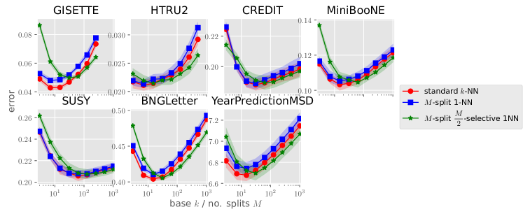
Figure C.2: Validation error profiles from 10-fold cross validation. Here, as expected, the optimal $M$ chosen for $(M,1)$-NN rules is in the same order of the optimal $k$ for the standard $k$-NN rules.

References

• Alabduljalil et al. (2013) Alabduljalil, M. A., Tang, X., and Yang, T. Optimizing parallel algorithms for all pairs similarity search. In Proc. Int. Conf. Web Search Data Mining, pp.  203–212, 2013.
• Anastasiu & Karypis (2019) Anastasiu, D. C. and Karypis, G. Parallel cosine nearest neighbor graph construction. J. Parallel. Distrib. Comput., 129:61–82, 2019.
• Angiulli & Pizzuti (2002) Angiulli, F. and Pizzuti, C. Fast outlier detection in high dimensional spaces. In Euro. Conf. Princ. Data Mining Knowledge Discov., pp. 15–27. Springer, 2002.
• Audibert et al. (2007) Audibert, J.-Y., Tsybakov, A. B., et al. Fast learning rates for plug-in classifiers. Ann. Statist., 35(2):608–633, 2007.
• Baldi et al. (2014) Baldi, P., Sadowski, P., and Whiteson, D. Searching for exotic particles in high-energy physics with deep learning. Nat. Commun, 5(1):1–9, 2014.
• Balsubramani et al. (2019) Balsubramani, A., Dasgupta, S., Freund, Y., and Moran, S. An adaptive nearest neighbor rule for classification. In Adv. Neural Inf. Process. Syst., volume 32, pp. 7579–7588, 2019.
• Bentley (1975) Bentley, J. L. Multidimensional binary search trees used for associative searching. Commun. ACM, 18(9):509–517, 1975.
• Beygelzimer et al. (2006) Beygelzimer, A., Kakade, S., and Langford, J. Cover trees for nearest neighbor. In Proc. Int. Conf. Mach. Learn., pp.  97–104, 2006.
• Bhattacharjee & Chaudhuri (2020) Bhattacharjee, R. and Chaudhuri, K. When are non-parametric methods robust? In Proc. Int. Conf. Mach. Learn., pp.  832–841, July 2020.
• Biau & Devroye (2015) Biau, G. and Devroye, L. Lectures on the Nearest Neighbor Method. Springer International Publishing, 2015.
• Biau et al. (2010) Biau, G., Cérou, F., and Guyader, A. On the rate of convergence of the bagged nearest neighbor estimate. J. Mach. Learn. Res., 11(Feb):687–712, 2010.
• Breiman (1996) Breiman, L. Bagging predictors. Mach. Learn., 24(2):123–140, 1996.
• Breiman (1999) Breiman, L. Pasting small votes for classification in large databases and on-line. Mach. Learn., 36(1):85–103, 1999.
• Chaudhuri & Dasgupta (2014) Chaudhuri, K. and Dasgupta, S. Rates of convergence for nearest neighbor classification. In Adv. Neural Inf. Process. Syst., volume 27, pp. 3437–3445. Curran Associates, Inc., 2014.
• Chen et al. (2018) Chen, G. H., Shah, D., et al. Explaining the success of nearest neighbor methods in prediction. Now Publishers, 2018.
• Cover (1968a) Cover, T. M. Estimation by the nearest neighbor rule. IEEE Trans. Inf. Theory, 14(1):50–55, 1968a.
• Cover (1968b) Cover, T. M. Rates of convergence for nearest neighbor procedures. In Proc. Hawaii Int. Conf. Sys. Sci., volume 415, 1968b.
• Cover & Hart (1967) Cover, T. M. and Hart, P. Nearest neighbor pattern classification. IEEE Trans. Inf. Theory, 13(1):21–27, 1967.
• Dasgupta & Kpotufe (2014) Dasgupta, S. and Kpotufe, S. Optimal rates for $k$-NN density and mode estimation. In Adv. Neural Inf. Process. Syst., volume 27, pp. 2555–2563. Curran Associates, Inc., 2014.
• Dasgupta & Kpotufe (2019) Dasgupta, S. and Kpotufe, S. Nearest-neighbor classification and search. In Roughgarden, T. (ed.), Beyond Worst-Case Analysis, chapter 1. Cambridge University Press, 2019.
• Datar et al. (2004) Datar, M., Immorlica, N., Indyk, P., and Mirrokni, V. S. Locality-sensitive hashing scheme based on p-stable distributions. In Proc. 20th Ann. Symp. Comput. Geom., pp.  253–262, 2004.
• Devroye et al. (1994) Devroye, L., Gyorfi, L., Krzyzak, A., and Lugosi, G. On the strong universal consistency of nearest neighbor regression function estimates. Ann. Statist., pp.  1371–1385, 1994.
• Devroye et al. (1996) Devroye, L., Györfi, L., and Lugosi, G. A probabilistic theory of pattern recognition, volume 31. Springer Science & Business Media, 1996.
• Dua & Graff (2019) Dua, D. and Graff, C. UCI Machine Learning Repository, 2019. URL http://archive.ics.uci.edu/ml.
• Duan et al. (2020) Duan, J., Qiao, X., and Cheng, G. Statistical guarantees of distributed nearest neighbor classification. In Adv. Neural Inf. Process. Syst., volume 33. Curran Associates, Inc., 2020.
• Efremenko et al. (2020) Efremenko, K., Kontorovich, A., and Noivirt, M. Fast and Bayes-consistent nearest neighbors. In Proc. Int. Conf. Artif. Int. Statist., pp.  1276–1286. PMLR, 2020.
• Fix & Hodges (1951) Fix, E. and Hodges, J. Discriminatory analysis: Nonparametric discrimination, consistency properties. Technical Report 4; 21-49-004, USAF School of Aviation Medicine, 1951.
• Fritz (1975) Fritz, J. Distribution-free exponential error bound for nearest neighbor pattern classification. IEEE Trans. Inf. Theory, 21(5):552–557, 1975.
• Fukunaga & Hostetler (1973) Fukunaga, K. and Hostetler, L. Optimization of $k$ nearest neighbor density estimates. IEEE Trans. Inf. Theory, 19(3):320–326, 1973.
• Gadat et al. (2016) Gadat, S., Klein, T., Marteau, C., et al. Classification in general finite dimensional spaces with the $k$-nearest neighbor rule. Ann. Statist., 44(3):982–1009, 2016.
• Gottlieb et al. (2014) Gottlieb, L.-A., Kontorovich, A., and Krauthgamer, R. Efficient classification for metric data (extended abstract COLT 2010). IEEE Trans. Inf. Theory, 60(9):5750–5759, 2014.
• Gottlieb et al. (2018) Gottlieb, L.-A., Kontorovich, A., and Nisnevitch, P. Near-optimal sample compression for nearest neighbors. IEEE Trans. Inf. Theory, 64(6):4120–4128, 2018.
• Gu et al. (2019) Gu, X., Akoglu, L., and Rinaldo, A. Statistical analysis of nearest neighbor methods for anomaly detection. In Adv. Neural Inf. Process. Syst., volume 32. Curran Associates, Inc., 2019.
• Guyon et al. (2004) Guyon, I., Gunn, S. R., Ben-Hur, A., and Dror, G. Result Analysis of the NIPS 2003 Feature Selection Challenge. In Adv. Neural Inf. Process. Syst., volume 4, pp.  545–552. Curran Associates, Inc., 2004.
• Gyorfi (1981) Gyorfi, L. The rate of convergence of $k_{n}$-nn regression estimates and classification rules. IEEE Trans. Inf. Theory, 27(3):362–364, 1981.
• Györfi & Weiss (2021) Györfi, L. and Weiss, R. Universal consistency and rates of convergence of multiclass prototype algorithms in metric spaces. J. Mach. Learn. Res., 22(151):1–25, 2021.
• Hall & Samworth (2005) Hall, P. and Samworth, R. J. Properties of bagged nearest neighbour classifiers. J. R. Stat. Soc. B, 67(3):363–379, 2005.
• Hanneke et al. (2020) Hanneke, S., Kontorovich, A., Sabato, S., and Weiss, R. Universal Bayes consistency in metric spaces. Ann. Statist., pp.  to appear, 2020.
• Har-Peled et al. (2012) Har-Peled, S., Indyk, P., and Motwani, R. Approximate nearest neighbor: Towards removing the curse of dimensionality. Theory Comput., 8(1):321–350, 2012.
• Hastie et al. (2009) Hastie, T., Tibshirani, R., and Friedman, J. The elements of statistical learning: data mining, inference, and prediction. Springer Science & Business Media, 2009.
• Heinonen (2012) Heinonen, J. Lectures on analysis on metric spaces. Springer Science & Business Media, 2012.
• Indyk & Motwani (1998) Indyk, P. and Motwani, R. Approximate nearest neighbors: towards removing the curse of dimensionality. In Proc. Symp. Theory Comput., pp.  604–613, 1998.
• Kibriya & Frank (2007) Kibriya, A. M. and Frank, E. An empirical comparison of exact nearest neighbour algorithms. In Euro. Conf. Princ. Data Mining Knowledge Discov., pp. 140–151. Springer, 2007.
• Kontorovich & Weiss (2015) Kontorovich, A. and Weiss, R. A Bayes consistent 1-NN classifier. In Lebanon, G. and Vishwanathan, S. V. N. (eds.), Proc. Int. Conf. Artif. Int. Statist., volume 38 of Proc. Mach. Learn. Res., pp.  480–488, San Diego, California, USA, 09–12 May 2015. PMLR.
• Kontorovich et al. (2017) Kontorovich, A., Sabato, S., and Weiss, R. Nearest-neighbor sample compression: Efficiency, consistency, infinite dimensions. In Adv. Neural Inf. Process. Syst., volume 30, pp. 1572–1582. Curran Associates, Inc., 2017.
• Kozachenko & Leonenko (1987) Kozachenko, L. F. and Leonenko, N. N. Sample estimate of the entropy of a random vector. Probl. Inf. Transm., 23(2):9–16, 1987. (Russian).
• Kpotufe & Verma (2017) Kpotufe, S. and Verma, N. Time-accuracy tradeoffs in kernel prediction: controlling prediction quality. J. Mach. Learn. Res., 18(1):1443–1471, 2017.
• Kulkarni & Posner (1995) Kulkarni, S. R. and Posner, S. E. Rates of convergence of nearest neighbor estimation under arbitrary sampling. IEEE Trans. Inf. Theory, 41(4):1028–1039, 1995.
• Leonenko et al. (2008) Leonenko, N., Pronzato, L., and Savani, V. A class of Rényi information estimators for multidimensional densities. Ann. Statist., 36(5):2153–2182, October 2008.
• Liu et al. (2021) Liu, R., Xu, G., and Shang, Z. Distributed adaptive nearest neighbor classifier: Algorithm and theory. arXiv preprint arXiv:2105.09788, 2021.
• Loftsgaarden & Quesenberry (1965) Loftsgaarden, D. O. and Quesenberry, C. P. A nonparametric estimate of a multivariate density function. Ann. Math. Statist., 36(3):1049–1051, 1965.
• Lyon et al. (2016) Lyon, R. J., Stappers, B., Cooper, S., Brooke, J., and Knowles, J. Fifty years of pulsar candidate selection: From simple filters to a new principled real-time classification approach. Mon. Not. R. Astron. Soc, 459(1):1104–1123, 2016. Data doi: 10.6084/m9.figshare.3080389.v1.
• Mack & Rosenblatt (1979) Mack, Y. and Rosenblatt, M. Multivariate k-nearest neighbor density estimates. J. Multivar. Anal., 9(1):1–15, 1979.
• Pedregosa et al. (2011) Pedregosa, F., Varoquaux, G., Gramfort, A., Michel, V., Thirion, B., Grisel, O., Blondel, M., Prettenhofer, P., Weiss, R., Dubourg, V., Vanderplas, J., Passos, A., Cournapeau, D., Brucher, M., Perrot, M., and Duchesnay, E. Scikit-learn: Machine learning in Python. J. Mach. Learn. Res., 12:2825–2830, 2011.
• Qiao et al. (2019) Qiao, X., Duan, J., and Cheng, G. Rates of convergence for large-scale nearest neighbor classification. In Adv. Neural Inf. Process. Syst., volume 32, pp. 10768–10779. Curran Associates, Inc., 2019.
• Ramaswamy et al. (2000) Ramaswamy, S., Rastogi, R., and Shim, K. Efficient algorithms for mining outliers from large data sets. In Proc. ACM Int. Conf. Manag. Data, pp.  427–438, 2000.
• Samworth (2012) Samworth, R. J. Optimal weighted nearest neighbour classifiers. Ann. Statist., 40(5):2733–2763, 2012.
• Slaney & Casey (2008) Slaney, M. and Casey, M. Locality-sensitive hashing for finding nearest neighbors. IEEE Signal Process. Mag., 25(2):128–131, 2008.
• Sun et al. (2016) Sun, W. W., Qiao, X., and Cheng, G. Stabilized nearest neighbor classifier and its statistical properties. J. Am. Statist. Assoc., 111(515):1254–1265, 2016.
• Uhlmann (1991) Uhlmann, J. K. Satisfying general proximity/similarity queries with metric trees. Inf. Process. Lett., 40(4):175–179, 1991.
• Vanschoren et al. (2013) Vanschoren, J., van Rijn, J. N., Bischl, B., and Torgo, L. OpenML: Networked Science in Machine Learning. SIGKDD Explor., 15(2):49–60, 2013. doi: 10.1145/2641190.2641198.
• Wagner (1971) Wagner, T. Convergence of the nearest neighbor rule. IEEE Trans. Inf. Theory, 17(5):566–571, 1971.
• Wang et al. (2018) Wang, Y., Jha, S., and Chaudhuri, K. Analyzing the robustness of nearest neighbors to adversarial examples. In Proc. Int. Conf. Mach. Learn., pp.  5133–5142, 2018.
• Xue & Kpotufe (2018) Xue, L. and Kpotufe, S. Achieving the time of 1-NN, but the accuracy of $k$-NN. In Proc. Int. Conf. Artif. Int. Statist., pp.  1628–1636, 2018.