The ALPINE-ALMA [CII] Survey: the population of [CII]-undetected galaxies and their role in the $\mathrm{L_{[CII]}}$-SFR relation

The [CII] 158 $\mu$m emission line represents so far one of the most profitable tools for the investigation of the high-redshift galaxies in the early Universe. Being one of the brightest cooling lines in the rest-frame far-infrared regime of star-forming galaxies, it has been successfully exploited as a tracer of star-formation rate (SFR) in local sources. The picture is more complex at higher redshifts, where its usability in this context is still under investigation. Recent results from the ALMA Large Program to INvestigate [CII] at Early times (ALPINE) survey suggest that there is no (or weak) evolution of the L_[CII]-SFR relation up to $z\sim 6$ but their reliability is hampered by the presence of a large population of [CII] non-detected galaxies. In this work, we characterize the population of [CII] non-detections in ALPINE. By stacking their ALMA spectra, we obtain a signal detected at $\sim 5.1\sigma$, resulting in a [CII] luminosity of $\mathrm{log(L_{\mathrm{[CII]}}}/\mathrm{L_{\odot}})$ $\sim 7.8$. When combining this value with those from the [CII] detections, we find a $\mathrm{L_{[CII]}}$-SFR relation with a slope $b=1.14\pm 0.11$, in agreement within the uncertainties both with the linear relation found in the local Universe, and with the previous findings from ALPINE at $z\sim 5$. This suggests that the [CII] line can be considered a good tracer of star formation up to the distant Universe. Finally, we show that the galaxies of our sample that most deviate from the observed L_[CII]-SFR relation could suffer from a less precise redshift estimation, perhaps artificially reducing their [CII] luminosity. In this respect, we claim that there is no evidence in favour of a deficit of [CII] content in high-z galaxies, in contrast with earlier studies.

1 Introduction

Over the last years, observations of the [CII] line emission at 158 $\mu$m rest-frame in galaxies have progressively improved to the point of being able to characterize the first sources of light during or near the epoch of cosmic Reionization (e.g., Wagg et al. 2012; Carilli & Walter 2013; Wang et al. 2013; Capak et al. 2015; Pentericci et al. 2016; Carniani et al. 2018b; Smit et al. 2018; Hashimoto et al. 2019; Matthee et al. 2019; Bakx et al. 2020; Harikane et al. 2020; Le Fèvre et al. 2020; Bouwens et al. 2021; Fudamoto et al. 2021).

The widespread interest in detecting the [CII] emission from local and distant galaxies is highly justified. This is the brightest line arising from the rest-frame far-infrared (FIR) spectra of star-forming galaxies (SFGs), representing one of the main coolants of their interstellar medium (ISM; e.g., Stacey et al. 1991; Carilli & Walter 2013). The bulk of its emission originates from photo-dissociation regions (PDRs; Hollenbach & Tielens 1999), possibly tracing the formation of new stars from giant molecular clouds. However, given its low ionization potential (11.3 eV, compared to the 13.6 eV of neutral hydrogen), this line deserves a thoughtful physical interpretation as it can also trace the diffuse neutral medium (e.g., Wolfire et al. 2003; Vallini et al. 2015), the molecular (e.g., Zanella et al. 2018; Dessauges-Zavadsky et al. 2020) and ionized (e.g., Cormier et al. 2012) gas. Furthermore, there is evidence that [CII] can reasonably trace the total HI content of galaxies (Heintz et al. 2021). The continuum surrounding this line lies close to the peak of the FIR dust-emission, making detection easier and helping to constrain the total FIR luminosity and obscured star formation (e.g., Gruppioni et al. 2020; Khusanova et al. 2021; Pozzi et al. 2021). Moreover, the [CII] emission can provide important information on a variety of ISM properties, such as the star-formation rate (SFR; e.g., De Looze et al. 2014; Olsen et al. 2017), the presence of outflows (e.g., Gallerani et al. 2018; Ginolfi et al. 2020), and the kinematics of the ISM (e.g., Jones et al. 2021; Romano et al. 2021). Therefore, the comparison of [CII] observations with simulations is mandatory to disentangle the diverse processes that take place in galaxies, in order to understand how they shape the observed morphology and kinematics of the line (e.g., Vallini et al. 2017; Ferrara et al. 2019; Kohandel et al. 2019).

In this context, the ALMA Large Program to INvestigate [CII] at Early times (ALPINE) survey (Béthermin et al. 2020; Faisst et al. 2020; Le Fèvre et al. 2020) has recently provided the first statistically significant sample of high-redshift normal galaxies (i.e., lying along a well-defined “main-sequence” of galaxies, with a relatively tight dispersion ($<0.3$ dex) in the SFR versus stellar mass plane; e.g., Noeske et al. 2007; Rodighiero et al. 2011; Speagle et al. 2014) detected in [CII] at the end of the reionization epoch ($4.4<z<5.9$). ALPINE observed a sample of 118 SFGs selected in UV and with redshifts spectroscopically confirmed by previous campaigns (Le Fèvre et al. 2015; Tasca et al. 2017; Hasinger et al. 2018) in order to ensure precise detections of the [CII] line. In particular, considering as detections those galaxies with a [CII] emission $\geq 3.5\sigma$ (corresponding to a 95% sample purity), ALPINE reached a successful rate of 64%, resulting in 75 detections and 43 non-detections (Béthermin et al. 2020; Le Fèvre et al. 2020).

Béthermin et al. (2020) first investigated the $\mathrm{L_{[CII]}}$-SFR relation by taking advantage of the ALPINE continuum-detected galaxies. They computed the average SFRs in different [CII] luminosity bins as the sum of the UV rest-frame data (Faisst et al. 2020) and of the mean obscured SFRs derived through the stacking of the continuum data (i.e., $\rm SFR_{total}=SFR_{UV}+SFR_{IR}$). Their results are in good agreement with the local and predicted relations. Then, Schaerer et al. (2020) took advantage of the full ALPINE sample (including both [CII]-detected galaxies and upper limits on non-detections; see Section 4) to study the evolution of the $\mathrm{L_{[CII]}}$-SFR relation over cosmic time, and to understand if the [CII] line is a good tracer of SFR at high redshift as it is in the local Universe (e.g., De Looze et al. 2014; Pineda et al. 2014). They found that the [CII] luminosity of the ALPINE galaxies scales linearly with their total SFRs (as traced by the sum of UV and IR contributions; see Schaerer et al. 2020), with a slight steepening of the slope depending on the [CII] non-detections upper limits used (Béthermin et al. 2020). However, to fully establish the connection between $\mathrm{L_{[CII]}}$ and SFR in distant galaxies a more in depth investigation of the ALPINE non-detections is needed.

In this work, we derive the average properties of the population of [CII] undetected galaxies in ALPINE through line stacking and use them to investigate the [CII] as a tracer of SFR at high redshift, and to put additional constraints on the already thoroughly studied $\mathrm{L_{[CII]}}$-SFR relation (Schaerer et al. 2020).

The structure of the paper is the following: in Section 2 we introduce the available data and observations used to compute the [CII] line profile resulting from the average population of non-detections. The procedure adopted to obtain the stacked line is described in Section 3. The results are reported in Section 4 and discussed in Section 5, respectively. Summary and conclusions are provided in Section 6.

Throughout this work, we adopt a $\mathrm{\Lambda-CDM}$ cosmology with $H_{0}=70$ km s^-1 Mpc^-1, $\mathrm{\Omega_{m}}=0.3$ and $\mathrm{\Omega_{\Lambda}}=0.7$. Furthermore, we use a Chabrier (2003) initial mass function (IMF).

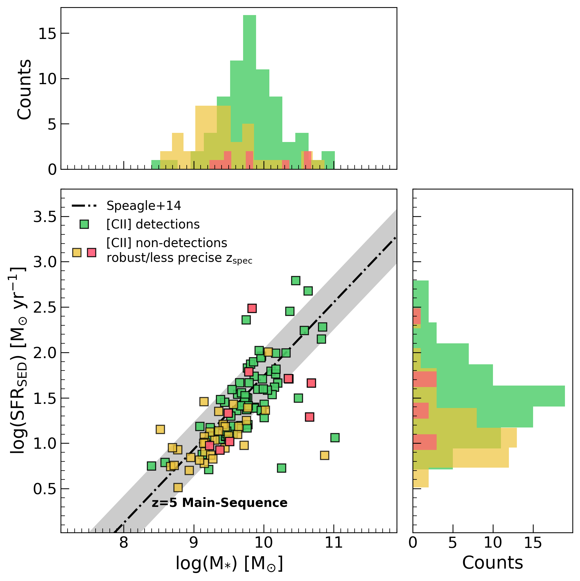
Figure 1: SFRs vs stellar masses of the ALPINE [CII]-detected (green squares) and undetected (yellow squares) galaxies. Red symbols represent [CII] non-detections with less precise spectroscopic redshift (see Section 2.2). The main-sequence of star-forming galaxies by Speagle et al. (2014) is shown as the black dot-dashed line, with its $\pm 0.3$ dex width represented by the grey shaded region. The top and right panels report the distributions in stellar mass and SFR, respectively, for both the detections and non-detections.

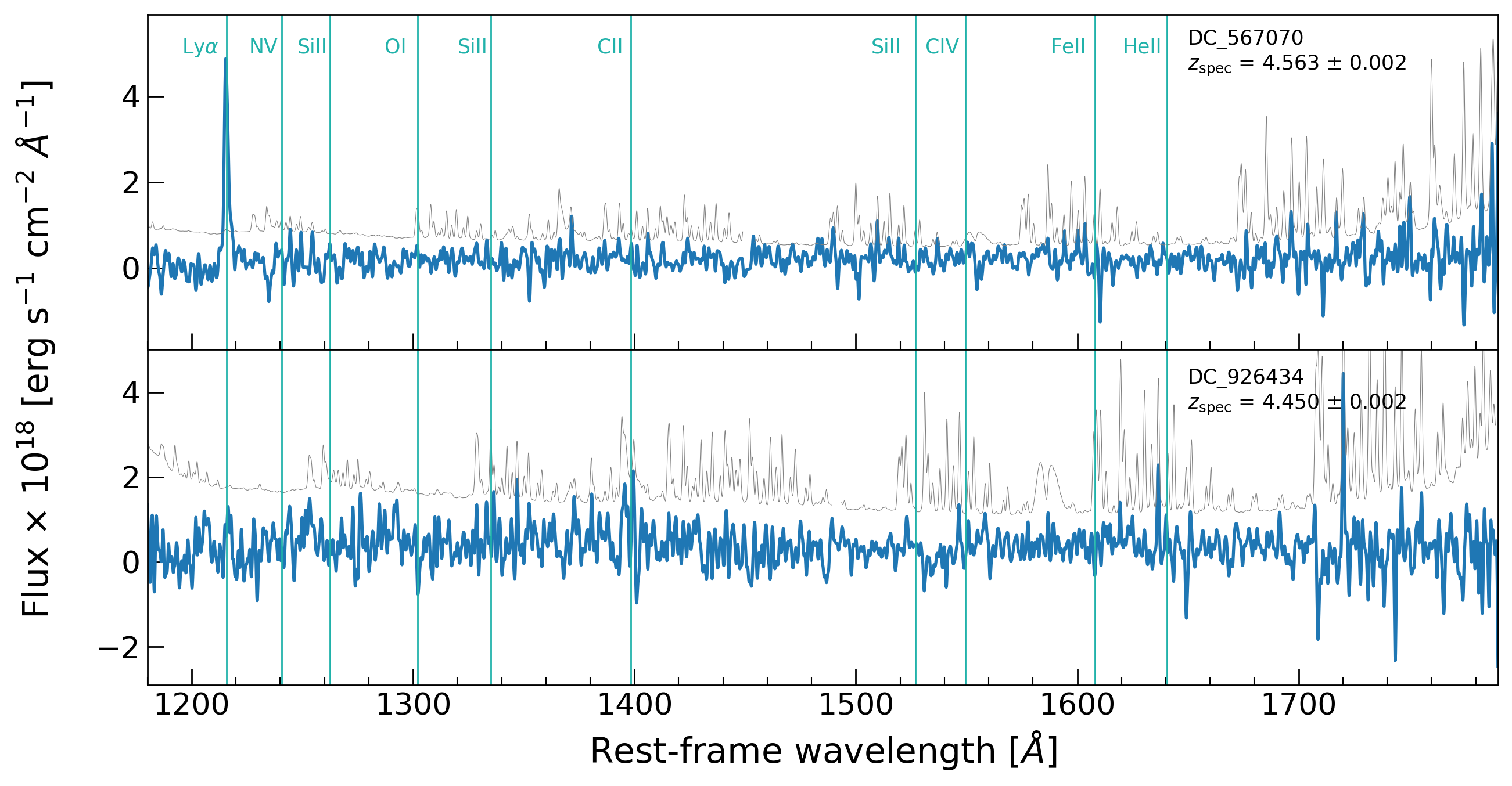
Figure 2: Examples of optical spectra of two [CII] non-detections with robust (top) and less precise (bottom) rest-frame UV spectroscopic redshift. The typical redshift uncertainty due to the spectral resolution (i.e., $\mathrm{R\sim 2700}$ from Hasinger et al. 2018) of the observations is also shown. Both panels report UV emission and absorption features, such as the Ly$\alpha$ line or the ISM Si II, C IV and He II absorption lines. The spectra (in blue) and the noise (in gray) are smoothed with a Gaussian filter with size of $2\leavevmode\nobreak\ \AA$ for a better visualization of the emission/absorption features.

2 Data and observations

2.1 Multi-wavelength and ALMA data

The ALPINE survey was designed to observe the [CII] line at 158 $\mu$m rest-frame and the surrounding FIR continuum emission from a sample of 118 SFGs at $4.4<z<5.9$, avoiding the redshift range $4.6<z<5.1$ due to a low-transmission atmospheric window. The campaign spent $\sim 70$ hours of observation in ALMA Band 7 (275-373 GHz) during cycles 5 and 6. The targets are drawn from the well-studied Cosmic Evolution Survey (COSMOS; Scoville et al. 2007a, b) and Extended Chandra Deep Field South (E-CDFS; Giavalisco et al. 2004; Cardamone et al. 2010) fields and have been observed in large optical/NIR spectroscopic campaigns such as VIMOS UltraDeep Survey (VUDS; Le Fèvre et al. 2015; Tasca et al. 2017) and DEIMOS 10K Spectroscopic Survey (Hasinger et al. 2018). They are selected in the rest-frame UV ($\mathrm{L_{UV}>0.6\leavevmode\nobreak\ L^{*}}$) and lie on the main-sequence, thus being representative of the average population of star-forming galaxies at $z\sim 5$ (e.g., Speagle et al. 2014). A wealth of multi-wavelength data is available for these sources, from the UV to the near-IR (e.g., Koekemoer et al. 2007; Sanders et al. 2007; McCracken et al. 2012; Guo et al. 2013; Nayyeri et al. 2017), allowing us to recover physical quantities such as stellar masses ($\mathrm{9\lesssim log(M_{*}/M_{\odot})\lesssim 11}$) and star-formation rates ($\mathrm{1\lesssim log(SFR/M_{\odot}yr^{-1})\lesssim 3}$) through spectral energy distribution (SED)-fitting (Faisst et al. 2020). Data are also available in the X-ray and radio bands (e.g., Hasinger et al. 2007; Smolčić et al. 2017).

The ALMA data-cubes were reduced and calibrated using the standard Common Astronomy Software Applications (CASA; McMullin et al. 2007) pipeline. Each cube was continuum-subtracted in the $uv$-plane in order to obtain line-only cubes with channel width of $\sim 25\leavevmode\nobreak\ \mathrm{km\leavevmode\nobreak\ s^{-1}}$ and beam size of $\sim 1^{\prime\prime}$ (with a pixel scale of $\sim 0.15^{\prime\prime}$; Béthermin et al. 2020). A line search algorithm was then applied to each continuum-subtracted cube resulting in 75 [CII] detections (signal-to-noise ratio; $\mathrm{S/N>3.5}$) and 43 non-detections. In Figure 1 we show the distributions of [CII]-detected and undetected galaxies along the $z\sim 5$ main-sequence of SFGs. The stellar masses and SFRs are those from the SED-fitting (Faisst et al. 2020). As evident, the ALPINE non-detections lie on the bottom-left side of the main-sequence, at lower stellar masses and SFRs with respect to those detected in [CII] (except for a few massive sources below the sequence).

For a more in-depth description of the overall ALPINE survey, the observations, data processing, and multi-wavelength analysis see Le Fèvre et al. (2020), Béthermin et al. (2020) and Faisst et al. (2020), respectively.

2.2 Rest-frame UV spectroscopic data

The 118 ALPINE galaxies have confirmed rest-frame UV spectroscopic redshifts from the VUDS (Le Fèvre et al. 2015; Tasca et al. 2015) and DEIMOS 10K (Hasinger et al. 2018) surveys. These are obtained both from the Ly$\alpha$ line and from UV rest-frame ISM absorption lines. However, these features are not always the best tracers of the systemic redshift of a source. The Ly$\alpha$ emission line is typically redshifted (with respect to the systemic velocity) because of the resonant scattering of the Ly$\alpha$ photons (e.g., Dijkstra 2014; Verhamme et al. 2015). On the opposite, ISM lines are usually blueshifted, suggesting the presence of outflowing gas (e.g., Steidel et al. 2010, 2018). The [CII] line is not affected by this kind of issues and, in principle, it can be used to stack together the ALMA spectra of the ALPINE non-detections to search for a significant signal. Moreover, it is not absorbed by dust and can be observed across the entire galaxy, resulting in a better tracer of the systemic redshift than optical nebular lines (e.g., Cassata et al. 2020; Faisst et al. 2020).

We do not have the systemic redshift information for the 43 ALPINE non-detections, therefore we can just rely on their UV redshifts. In particular, we need to know the UV spectroscopic redshifts of our sources with good accuracy, in order to exclude objects with less precise redshift estimates for which the [CII] line could lie outside of the ALMA observational window or that could alter the $\Delta v_{\mathrm{Ly}\alpha}$ statistics in our stacking analysis (see Section 3). For this reason, we visually inspected the optical spectra of the non-detections. We found that 34 out of 43 sources present multiple high S/N spectral features, all of them showing a prominent Ly$\alpha$ line in emission, allowing for a precise and accurate estimate of their spectroscopic redshifts. The remaining 9 galaxies have very weak or no Ly$\alpha$ in emission and less prominent and sharp UV absorption lines. Although it is likely that the redshift is generally accurate for these sources as well, we decide to exclude them from our stacking analysis, in order not to include additional uncertainties due to possible strong [CII] offsets with respect to the expected position of the line. Figure 2 reports an example of UV/optical spectra of two [CII] non-detections with a robust and less precise spectroscopic redshift, respectively. In the first case, the galaxy shows a clear Ly$\alpha$ line in emission and some other possible absorption features at longer wavelengths that provide a precise estimate of the spectroscopic redshift. On the other hand, the spectrum of the second source is quite noisy, with fewer recognizable spectral features. We thus obtain a final sample of 34 [CII] non-detections. The rest-frame UV and ALMA emissions of these galaxies are shown in Figure 3, where it is evident that no significant [CII] signal is present in these sources. The 9 galaxies with less precise $z_{\mathrm{spec}}$ are also reported for completeness in Figure 1 as red squares.

For these reasons, in the following analysis, we make use of the redshift obtained from the peak of the Ly$\alpha$ line, and then correct it for the observed velocity offsets between Ly$\alpha$ and the systemic velocity traced by [CII] ($0<\Delta v_{\mathrm{Ly}\alpha}<400$ km s^-1) for the ALPINE detections (Cassata et al. 2020).

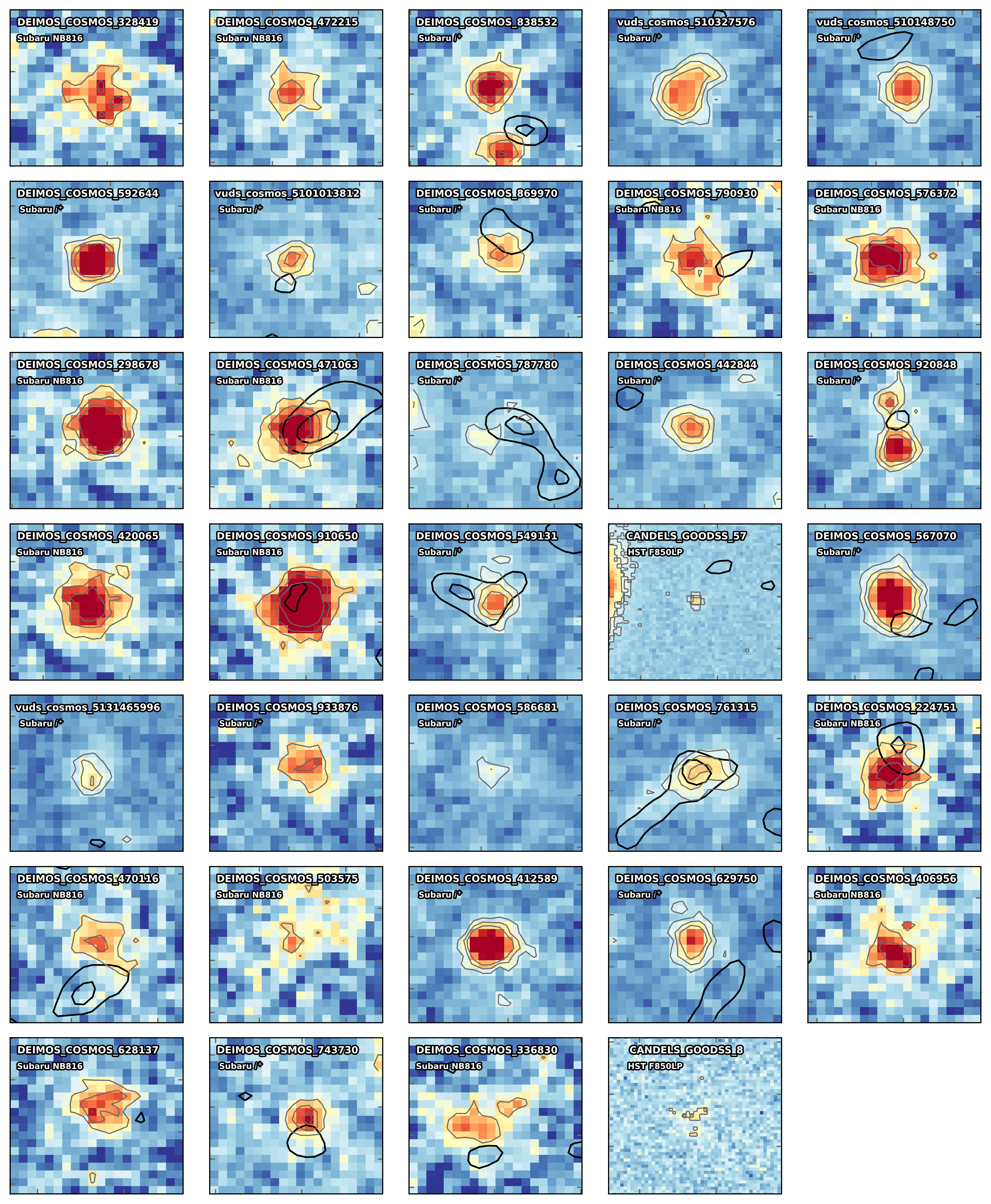
Figure 3: Cutouts of the 34 [CII] non-detections centered on their optical positions. Depending on the method used to pre-select each galaxy before the spectroscopic observation, i.e., Lyman-break, Ly$\alpha$, or $i$-band dropout selection, we show the emission from the Subaru broad-band $i^{+}$ and narrow-band NB816 filters (Taniguchi et al. 2007, 2015; Laigle et al. 2016), or from the HST/ACS F850LP (Giavalisco et al. 2004), respectively (see Faisst et al. 2020). Each image is $3^{\prime\prime}\times 3^{\prime\prime}$ wide. Grey contours show 3, 5, and 7$\sigma$ optical emission. Black contours (if present) represent 2 and 3$\sigma$ ALMA [CII] emission. The name of each non-detection, as well as the filter used, are reported in the upper-left corner of the corresponding cutout.

3 Stacking of non-detections

We proceed with a mean stacking of the ALMA spectra of the 34 ALPINE [CII] non-detections to search for a signal emerging from the noise of individual galaxies.

In principle, the stacking analysis can be done both in the image and uv planes. In the first case, it is possible to perform both 1D and 3D stacking through the extraction of individual spectra and by exploring the full data-cubes, respectively (e.g., Bischetti et al. 2019; Stanley et al. 2019). 2D stacking can be performed as well, by aligning and summing intensity maps of different sources (e.g., Méndez-Hernández et al. 2020). The stacking in the uv plane is instead based on the analysis of the visibility data associated to the emission line in the Fourier space, before the imaging process (e.g., Fujimoto et al. 2019; Carvajal et al. 2020). Lindroos et al. (2015) made use of several simulated uv continuum data sets to compare the performances of image and uv stacking. They found that the two procedures yield similar results within the uncertainties, although in some cases stacking in the uv plane could lead to higher S/N, also avoiding possible issues during the deconvolution process from the Fourier to the image domain. Méndez-Hernández et al. (2020) also made a comparison between the image and uv stacking of CO emission lines in a sample of 27 low-$z$ SFGs drawn from the Valparaíso ALMA/APEX Line Emission Survey (VALES; Villanueva et al. 2017; Cheng et al. 2018). They retrieved similar flux densities with both methods, with the uv stacking producing similar or slightly higher S/N as compared to the image one, depending on the brightness of the line. Regardless of the adopted method, all the above techniques need a good knowledge of the systemic redshift of the source. Furthermore, to select the spectral channels including the emission line in the case of uv stacking or for the production of the intensity maps, an estimate of the full width at half maximum (FWHM) of each source is also required. In the analysis of the ALPINE [CII] undetected galaxies, we do not know at which frequency the expected line is (because of the observed velocity offset between Ly$\alpha$ and [CII]), and we do not have any information on the FWHM of each source. For these reasons, and considering that both image and uv planes provide similar results, we decide to proceed with a 1D spectral stacking of the [CII] non-detections starting from the image plane.

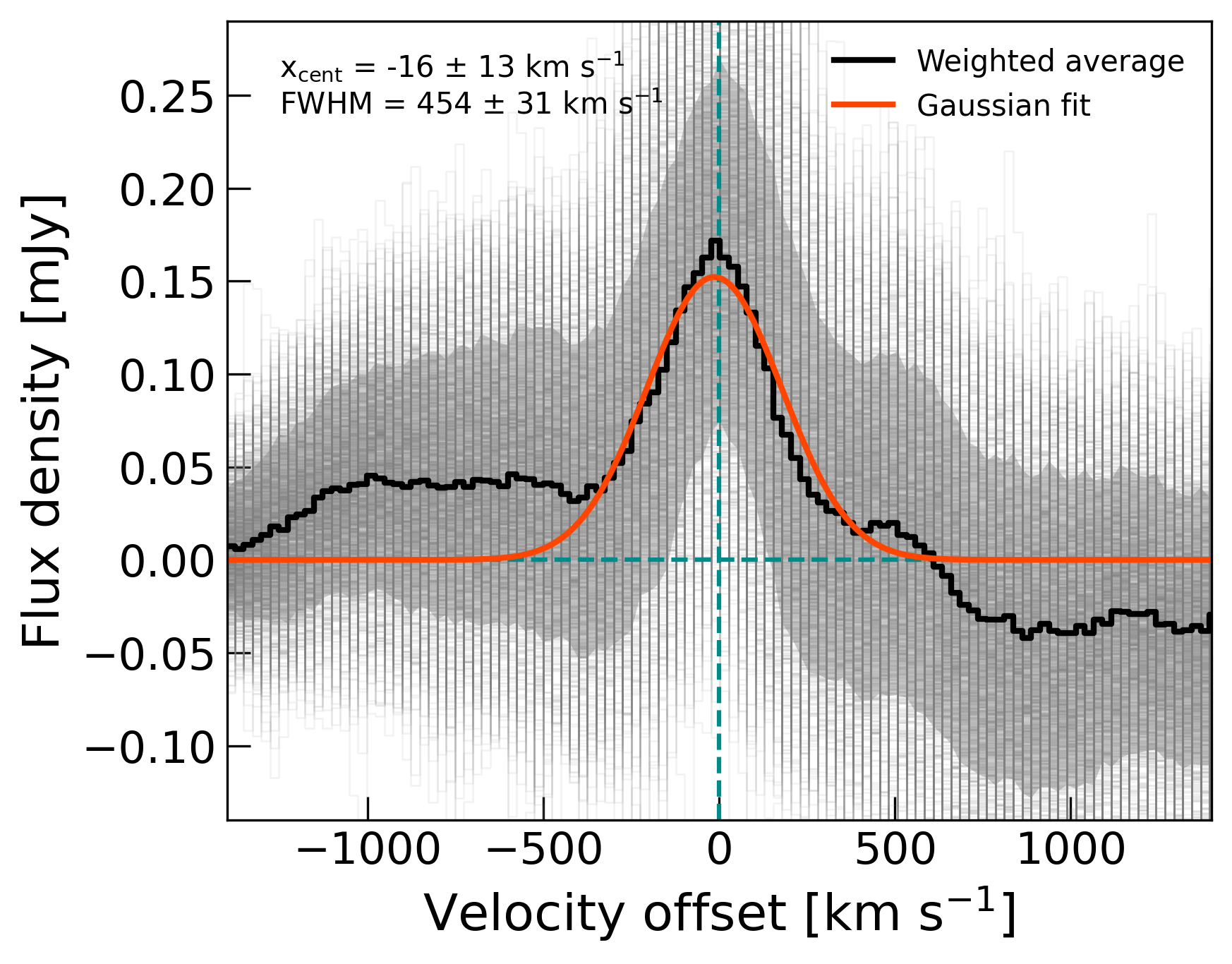
Figure 4: Average spectrum of the ALPINE [CII] non-detections weighted for the S/N of the individual stacked spectra with $\mathrm{FWHM}\leq 400$ km s^-1 (solid black line). The thin lines represent the individual realizations after taking into account the observed shift between the [CII] and Ly$\alpha$ lines (Cassata et al. 2020). The solid red line represents the Gaussian fit on the average line profile. The shaded area shows the uncertainty associated to the average line profile as taken from the 16th and 84th percentiles of the 1000 spectra distribution. The dashed dark cyan lines mark the zero flux and velocity offset levels. The centroid and FWHM computed from the Gaussian fit on the average line profile are shown on the top left corner.

In particular, we extract each spectrum from the original data-cubes of the ALPINE data release 1 (DR1; Béthermin et al. 2020), within a fixed aperture of 1” of radius (defining the central regions of the ALPINE targets; see Béthermin et al. 2020) centered at the optical position of the source, and covering a spectral range of $\sim 3$ GHz around the expected peak frequency of the emission line (as traced by the Ly$\alpha$ emission). At first, we use the Ly$\alpha$-based spectroscopic redshifts of the non-detections to align them to the same reference frame, and then we stack them together. Because the Ly$\alpha$ line is typically shifted to the red relative to the systemic redshift as defined by the [CII] line (Cassata et al. 2020), it is likely that our stacked emission is offset from the systemic by some amount. Further, the velocity offset between Ly$\alpha$ and systemic is not constant, but is rather a complicated function of various physical conditions within a given galaxy (e.g., Erb et al. 2004; Pentericci et al. 2016; Marchi et al. 2019), meaning that the signal recovered in a stack where these offsets were not accounted for would be broadened and dampened. For these reasons, we apply to each source a spectral offset randomly extracted from the $\Delta v_{\mathrm{Ly}\alpha}$ distribution obtained by Cassata et al. (2020) from a sub-sample of the ALPINE detections, and then compute the mean stack on the shifted spectra. Certainly, by drawing random values out of the $\Delta v_{\mathrm{Ly}\alpha}$ we expect to introduce an artificial broadening of the stacked line, as well. In particular, the further (nearer) the rest-frame UV spectroscopic redshift (as traced by the Ly$\alpha$ line) from the systemic one (as traced by the [CII] line), the wider (narrower) the stacked line. To avoid this issue, we compute each time a Gaussian fit on the stacked line, estimating its full width at half maximum as $\mathrm{FWHM}=2.355\sigma$, where $\sigma$ is the standard deviation of the Gaussian. For each stacked spectrum, we then require that $\mathrm{FWHM}\leq 400$ km s^-1, which defines the 84th percentile of the observed FWHM distribution of the ALPINE [CII] detections (see Béthermin et al. 2020), until reaching 1000 realizations.

We show the result of this procedure in Figure 4, where the grey histograms represent the spectra that satisfy the above requirements on the FWHM. To produce the averaged line profile, we weight each realization of the stacked spectra in different ways. We assume $w=1$ in case of no weighting, $w=1/\sigma_{rms}^{2}$ for an inverse-variance weighting (where $\sigma_{rms}$ is the standard deviation of each stacked spectrum), and $w=\mathrm{S/N}$ to weight each stacked spectrum by its S/N. In the latter case, we estimate the S/N as the ratio between the peak flux of the stacked line and the standard deviation of the spectral channels at velocities greater and smaller than $\pm 600$ km s^-1 from the peak, in order to avoid contamination from the stacked emission line. The line profiles obtained by applying these different weightings are similar to each other, although resulting in a slightly higher S/N for the case with $w=\mathrm{S/N}$. For this reason, we decide to show in Figure 4 only the average stacked spectrum obtained by weighting each realization by its S/N.

We then check the effect of the random extraction on the final average stacked profile, by making the following test. We select a sub-sample of [CII] detections having, in addition to the [CII]-traced systemic redshift, also the redshift measurements from Ly$\alpha$. We first stack together the ALMA spectra basing on their systemic redshifts (i.e., without applying any spectral offset), to obtain the real FWHM and flux of the line. Then, we repeat the stacking by using our method, i.e., by extracting random shifts from the $\Delta v_{\mathrm{Ly\alpha}}$ distribution, and compare the two results. We find that the random extraction method produces a $\sim 2$ times broader FWHM than the true value computed by stacking the spectra at their correct wavelengths. At the same time, there is no significant difference in the retrieved S/N and integrated fluxes. As an additional check, we re-do the entire stacking procedure by considering, for each source, the mean value of the Ly$\alpha$-[CII] offset distribution found by Cassata et al. (2020) (i.e., $\sim 183\leavevmode\nobreak\ \mathrm{km\leavevmode\nobreak\ s^{-1}}$), obtaining a FWHM $\sim 150\leavevmode\nobreak\ \mathrm{km\leavevmode\nobreak\ s^{-1}}$ narrower than what previously found. On the other hand, the integrated flux and S/N of the resulting line are slightly lower, but still comparable, than those computed by assuming the random $\Delta v_{\mathrm{Ly}\alpha}$ offsets. This further suggests that the random extraction has only a significant effect on the FWHM of the stacked line. Therefore, we are confident that the stacking method used in this work does not under/overestimate the true value of the [CII] luminosity of the non-detections population under study.

By fitting the stacked line profile with a Gaussian function, we find the signal peaking at $\mathrm{x_{cent}}=-16\pm 13$ km s^-1, consistent with the systemic velocity traced by the [CII] line, and having $\mathrm{FWHM}=454\pm 31$ km s^-1. The computed S/N is $\sim 5.1$, revealing the presence of an underlying population of [CII] emitters likely suffering from low S/N (in terms of [CII] emission) possibly caused by the low SFRs and stellar masses which characterize them (see Figure 1). Following Solomon et al. (1992), we also compute $\mathrm{L_{[CII]}}$ as

$$\mathrm{L_{[CII]}}=1.04\times 10^{-3}\leavevmode\nobreak\ S_{\mathrm{[CII]}}\leavevmode\nobreak\ \Delta v\leavevmode\nobreak\ D_{L}^{2}\leavevmode\nobreak\ \nu_{obs}\leavevmode\nobreak\ [\mathrm{L_{\odot}}],$$ (1)

where $S_{\mathrm{[CII]}}\leavevmode\nobreak\ \Delta v$ is the velocity-integrated line flux in units of Jy km s^-1, $D_{L}$ is the luminosity distance in Mpc at the median redshift of the sample (i.e., $z_{\mathrm{med}}=5.52$), and $\nu_{obs}$ is the observed peak frequency in GHz.

To attribute an uncertainty on the velocity-integrated flux (and hence on the [CII] luminosity) we perform a delete-$d$ jackknife resampling (Shao & Wu 1989). We produce 500 jackknife realizations following the same method described above, but randomly removing each time 20% of the 34 spectra in the parent sample and computing again the integrated flux of the stacked spectra. The error on $S_{\mathrm{[CII]}}\leavevmode\nobreak\ \Delta v$ is then computed from the 16th and 84th percentiles of the fluxes distribution of the 500 jackknife realizations. As a result, we obtain $S_{\mathrm{[CII]}}\leavevmode\nobreak\ \Delta v=(73\pm 11)\times 10^{-3}$ Jy km s^-1.

We thus find $\mathrm{log(L_{\mathrm{[CII]}}}/\mathrm{L_{\odot}})=7.8\pm 0.3$, where the error is computed by propagating the uncertainty on the [CII] flux and the redshift on Equation 1. We test that this result is not significantly different from the one obtained by removing the constraint on the FWHM of the stacked spectra, which thus affects only the width of the line.

Furthermore, given the wide range spanned by the [CII] non-detections both in stellar mass (i.e., $\mathrm{9\lesssim log(M_{*}/M_{\odot})\lesssim 11}$) and star-formation rates (i.e., $\mathrm{0.5\lesssim log(SFR/M_{\odot}yr^{-1})\lesssim 2.0}$; see Figure 1), we decide to split our sample in two bins of SFR to check if the above result from stacking is dominated by the most massive and star-forming sources. We use the median SFR of the sample ($\mathrm{log(SFR_{TOT,med}/M_{\odot}\leavevmode\nobreak\ yr^{-1}})=1.16$; as defined in Section 4) to make two bins composed of 17 objects each, repeating for both of them the previously described stacking procedure. We do not find any significant emission in the low-SFR bin. On the contrary, a S/N $\sim 6.8$ emission is produced in the high-SFR bin, suggesting that most of the signal in Figure 4 is due to the most massive SFGs. By adopting the above-described stacking procedure on the whole sample, we find $\mathrm{log(L_{\mathrm{[CII]}}}/\mathrm{L_{\odot}})=8.0\pm 0.2$ in the high-SFR bin. In the lower bin with no detection, we consider instead the average of the [CII] non-detections with robust spectroscopic redshift, computed as the addition in quadrature of the corresponding [CII] upper limits divided by the square root of the number of sources in the bin (e.g., Cohen 1988), finding $\mathrm{log(L_{\mathrm{[CII]}}}/\mathrm{L_{\odot}})\lesssim 7.8$. We show these results in Figure 5, along with the previous result from the stacking of all the [CII] non-detections.

Finally, Figure 4 shows that the average [CII] profile presents a negative (positive) continuum at the right (left) of the line. By analyzing each spectrum individually, we attribute this behaviour to different sources that present a negative (positive) continuum at positive (negative) velocity offset with respect to the expected line. However, we believe that this issue is only due to statistical fluctuations originated from the small size of the sample, rather than to calibration problems in the ALMA data reductions or physical processes in these sources. This is also confirmed by the dispersion of the 1000 realizations of the stacked line in the figure, which shows that the above-mentioned continuum levels are not significant and consistent with zero.

4 Results

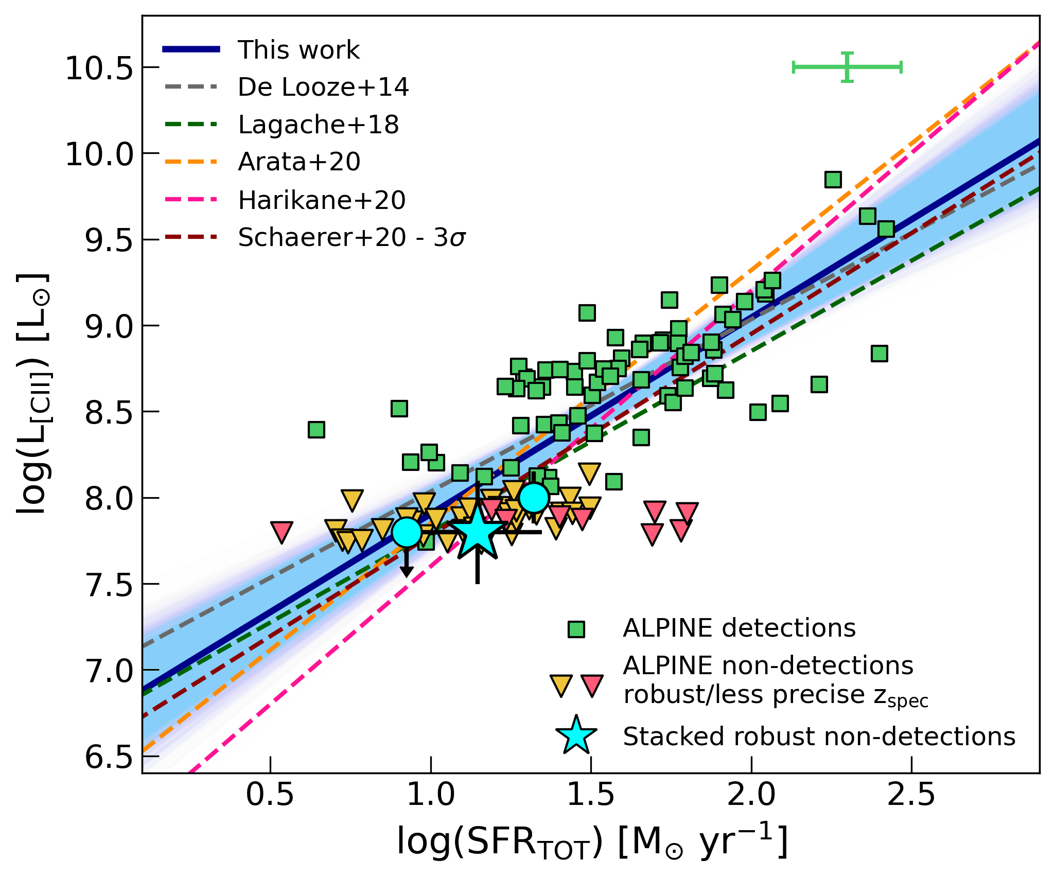
Figure 5: [CII] luminosity as a function of total SFR (UV+FIR; see text) for the ALPINE detections (green squares) and non-detections (as $3\sigma$ upper limits; yellow triangles). The red markers represent the [CII]-undetected galaxies with less precise $z_{\mathrm{spec}}$ (see Section 2). The green errobars in the upper right corner show the average uncertainties of [CII] detections on both L_[CII] and SFR. The cyan big star shows the result of this work for the stacked non-detections, with the error on L_[CII] computed as described in Section 3. The cyan circles are the [CII] upper limit and detection found in the low- and high-SFR bins introduced in the text, respectively. We also report different L_[CII]-SFR relations from the literature: the local relation by De Looze et al. (2014) (dashed gray line), the predicted relation by the models of Lagache et al. (2018) at $z\sim 5$ (dashed green line), the predicted relation by Arata et al. (2020) for galaxies at $z>6$ (dashed yellow line), the fitted relation by Harikane et al. (2020) on $z>6$ galaxies (dashed pink line), the latest results obtained by Schaerer et al. (2020) at $z\sim 5$ with ALPINE considering non-detections as $3\sigma$ upper limits (dashed red line). Finally, the solid blue line and shaded area report our best-fit and uncertainties to the [CII] detections + stacked robust non-detections.

By taking advantage of the [CII] luminosity computed from the stack of the ALPINE non-detections, we explore the relation between $\mathrm{L_{[CII]}}$ and SFR in these galaxies in order to compare them to the results obtained for the combined [CII] detections and non-detections upper limits (Schaerer et al. 2020).

Following Schaerer et al. (2020), we report in Figure 5 the [CII] luminosities and SFRs of the ALPINE detections and non-detections (as 3$\sigma$ upper limits; see also Figure 4 by Schaerer et al. 2020). Contrarily to Figure 1 in which we show the SFRs obtained through SED-fitting (for consistency with the stellar mass values obtained with the same procedure; Faisst et al. 2020), we use in this case the total SFRs obtained as $\mathrm{SFR_{TOT}=SFR(UV)+SFR(IR)}$, where SFR(UV) comes from the observed UV absolute magnitude at 1500 $\AA$, and SFR(IR) is obtained both through the ALMA continuum measurements and, for galaxies undetected in continuum, through predictions of the IRX-$\beta$ relation by Fudamoto et al. (2020), obtained from a stacking analysis of all ALMA continuum images, including both individual detections and non-detections. In this way, we are able to compare our results with those previously found in ALPINE by Schaerer et al. (2020) and with other $\mathrm{L_{[CII]}}$-SFR relations already present in the literature. Among these, we show: i) the local $\mathrm{L_{[CII]}}$-SFR relation found by De Looze et al. (2014) for a sample of low-z HII/starburst galaxies; ii) the predicted relation found by Lagache et al. (2018) at $z=5$; iii) the predictions from simulations for $z>6$ galaxies by Arata et al. (2020); iv) the relation found by Harikane et al. (2020) for galaxies observed in [CII] at $6<z<9$; iv) the relation fitted to the ALPINE data only (including 3$\sigma$ upper limits on non-detections) by Schaerer et al. (2020). Furthermore, we show our results from the stacking of ALPINE [CII] non-detections (i.e., $\mathrm{log(L_{\mathrm{[CII]}}}/\mathrm{L_{\odot}})=7.8\pm 0.3$), adopting their mean $\mathrm{SFR_{TOT}}$ (i.e., $\mathrm{log(SFR_{TOT,mean}/M_{\odot}\leavevmode\nobreak\ yr^{-1}})=1.14\pm 0.20$, that is also in good agreement with the upper limit found by Béthermin et al. (2020) by stacking the ALMA continuum of the [CII] non-detections. For further information, see their Section 7.5). For comparison, we also report the [CII] upper-limit and detection found in the low- and high-SFR bin respectively, as described in Section 3.

Our $\mathrm{L_{\mathrm{[CII]}}}$ value is consistent with the $3\sigma$ upper limits found by Béthermin et al. (2020) and used by Schaerer et al. (2020) in their analysis. This result suggests that the [CII] non-detections are not drawn from a different population of galaxies with respect to the ALPINE detections. Rather, these are galaxies lying on the bottom-left region of the $z\sim 5$ main-sequence with lower SFRs and stellar masses, and possibly with fainter [CII] emission (see also Section 5 for possible caveats causing low [CII] content in high-$z$ galaxies).

We fit the combined [CII] luminosity and SFR from the stacking of non-detections with the ALPINE [CII]-detected galaxies with a linear relation of the form

$$\mathrm{log(L_{\mathrm{[CII]}}/L_{\odot})}=a+b\times\mathrm{log(SFR/M_{\odot}\leavevmode\nobreak\ yr^{-1}}),$$ (2)

where $a$ and $b$ are the intercept and slope of the relation, respectively. For consistency with Schaerer et al. (2020), we use the linmix package by Kelly (2007) which makes use of a Bayesian approach to account for measurement errors in both variables in linear regressions. The errors on the [CII] luminosities are taken from Béthermin et al. (2020) for the ALPINE detections, and from the stacking for the non-detected sources. Regarding the individual uncertainties on the SFRs, we propagate the errors of SFR(UV) and SFR(IR) on the total SFR (obtaining on average $\sim 0.2$ dex for both detections and non-detections).

With our stacked non-detections, we obtain a best-fit relation with $a=6.76\pm 0.17$ and $b=1.14\pm 0.11$. This is consistent with the slope obtained from local galaxies ($b=1.00\pm 0.04$; De Looze et al. 2014), and in agreement with that previously found by Schaerer et al. (2020) considering detections and $3\sigma$ upper limits on non-detections (i.e., $b=1.17\pm 0.12$). Table 1 summarizes the parameters describing the L_[CII]-SFR relations found in the literature and in this work.

Table 1: Summary of L_[CII]-SFR relations from the literature and from this work, as parameterized in Equation 2.

Literature	Sample	Redshift	a	b
(1)	(2)	(3)	(4)	(5)
De Looze et al. (2014)	HII/starburst	$<0.5$	$7.06\pm 0.33$	$1.00\pm 0.04$
Lagache et al. (2018)	G.A.S. + CLOUDY	4 - 6	$6.75\pm 0.07$	$1.05\pm 0.07$
Arata et al. (2020)	GADGET-3 + ART2	¿6	6.38	1.47
Harikane et al. (2020)	LBGs/SMGs	6 - 9	6.00	1.60
Schaerer et al. (2020)	ALPINE ($3\sigma$ limits)	4 - 6	$6.61\pm 0.20$	$1.17\pm 0.12$
This work	ALPINE det + stacked non-det	4 - 6	$6.76\pm 0.17$	$1.14\pm 0.11$

5 Discussion

A large scatter in the $\mathrm{L_{[CII]}}$-SFR relation is in place for sources at $z>4$ (i.e., $\gtrsim 0.4$ dex, that is $\sim 2$ times larger than the intrinsic dispersion of local galaxies; Carniani et al. 2018a; Schaerer et al. 2020). Such a scatter is produced by the multitude of [CII] detections and non-detections now available in the high-$z$ Universe, and could be due both to different physical conditions in the ISM of distant galaxies, or to systematic in the [CII] and SFR derivation.

Jolly et al. (2021) analyzed a sample of 52 gravitationally lensed galaxies at $z\gtrsim 6$ as part of the ALMA Lensing Cluster Survey (ALCS) searching for [CII] emission through spectral stacking. They found no [CII] detection in their sample, providing $3\sigma$ upper limits on the [CII] luminosity of $\mathrm{log(L_{\mathrm{[CII]}}}/\mathrm{L_{\odot}})<7-8$, depending on the considered sub-sample (e.g., sources with high SFR, or with secure spectroscopic redshift) and stacking method (i.e., weighted mean and median stacking). Their findings are comparable with (or lower than) our average [CII] luminosity from the ALPINE non-detections (i.e., $\mathrm{log(L_{\mathrm{[CII]}}}/\mathrm{L_{\odot}})=7.8\pm 0.3$). However, these authors claim that the [CII] upper limits they found could be underestimated because some potential biases in the analyzed galaxy sample. First, they do not account for the spectroscopic offset between Ly$\alpha$ and [CII] that, as mentioned in Section 3, could alter the stacked line profile and lower the average amount of [CII] luminosity arising from non-detections. Astrometric offsets between ALMA and ancillary data could affect the [CII] luminosity estimate, as well. This issue was well-studied by many authors in the literature (e.g., Dunlop et al. 2017; Franco et al. 2018), and in ALPINE by Faisst et al. (2020) and Fujimoto et al. (2020), who found a typical shift between [CII] and UV rest-frame emission of 0.15” (corresponding to $\sim 1$ kpc at $z=5$). We overcome this problem by considering a fixed aperture of 1” of radius to extract the ALMA spectra of the [CII] non-detections (which is also $\sim 3$ times larger than the typical [CII] size of individual detections in ALPINE, i.e., 2.1 kpc). The surface brightness distribution of the [CII] emission and its FWHM could also reduce the [CII] luminosity and cause non-detections. For instance, Fujimoto et al. (2020) found that [CII] emission is typically 2-3 times more extended than rest-frame UV emission, which could result in a large underestimation of the total [CII] flux, depending on the resolution of the observations (e.g., Carniani et al. 2020). Kohandel et al. (2019) studied instead the effect of FWHM and inclination of the galaxy on the [CII] detectability, finding that an edge-on galaxy with a large line width (i.e., FWHM $>400$ km s^-1) could result in a non-detection, biasing the [CII] luminosity estimates in high-$z$ sources. Finally, Jolly et al. (2021) noticed that their results may be lowered by the presence of a large number of Ly$\alpha$ emitters in their sample, that could in principle have small content of dust, resulting in low [CII] and FIR emission. This issue has been minimized in the ALPINE sample by a heterogeneous pre-selection of the spectroscopically observed galaxies done with a variety of diverse selection methods (Faisst et al. 2020). In addition, Cassata et al. (2020) found that 44% of the ALPINE sources are Ly$\alpha$ emitters, with the probability of detecting [CII] not strongly dependent on the presence of bright Ly$\alpha$ emission.

Apart from the above caveats, the little [CII] content found by Jolly et al. (2021) in their galaxies could also be due to low metallicity levels. Indeed, many simulations show that low metallicity in high-$z$ galaxies could result in a lower Carbon abundance, and stronger radiation field that could decrease the [CII] content (e.g., Vallini et al. 2015; Ferrara et al. 2019; Vallini et al. 2020). About this, it is interesting to note that our L_[CII]-SFR slope (i.e., $b=1.14\pm 0.11$) is also consistent with that found by De Looze et al. (2014) for metal-poor dwarf galaxies in the local Universe (i.e., $b\sim 1.25$). This is in line with the results from Faisst et al. (2020) who compared the H$\alpha$ (which is a good tracer of the star-formation properties of galaxies) and [CII] luminosities for a sub-sample of the ALPINE galaxies. They found that bright [CII] galaxies are in good agreement with the local relation between H$\alpha$ and [CII] found by De Looze et al. (2014). However, for lower [CII] luminosities ($<5\times 10^{8}\leavevmode\nobreak\ \mathrm{L_{\odot}}$, as those probed by the [CII] non-detections), the galaxies seem to be more consistent with the relation found for local metal-poor dwarf galaxies, although with a large scatter. The possible effect of metallicity on [CII] is also suggested by the results of Faisst et al. (2020) who noticed that the strength of [CII] emission increases along the main-sequence, with a significant decrease of [CII] content in galaxies with $\mathrm{log(M_{*}/M_{\odot})<9.3}$ and $\mathrm{log(SFR/M_{\odot}yr^{-1})<1}$ (i.e., in [CII]-undetected sources). This further suggests that the metallicity of galaxies (along with the strength of their [CII] emission) could play an important role in the derivation of the L_[CII]-SFR relation (Vallini et al. 2015; Olsen et al. 2017; Lagache et al. 2018; Narayanan et al. 2018; Ferrara et al. 2019). Future investigations of this topic will be possible thanks to the forthcoming near- and mid-infrared observations of the James Webb Space Telescope, through which we will be able to provide measurements of the metallicity content of distant galaxies.

To better understand the relation between [CII] and SFR in normal $z\sim 5$ galaxies, we compare our result with those of different simulations. Lagache et al. (2018) used the semi-analytical model G.A.S. (Galaxy Assembly from dark-matter Simulations) in combination with the photoionization code CLOUDY (Ferland et al. 2013, 2017) to predict the [CII] luminosity of a large number of galaxies at $z\sim 5$. They found an average relation with a slope in agreement with the one by De Looze et al. (2014) for HII/starburst galaxies at low redshift, but that is dependent on several parameters, such as the metallicity of the galaxies and the intensity of their interstellar radiation field. More recently, Arata et al. (2020) combined cosmological hydrodynamic simulations performed with the GADGET-3 code (Springel 2005), with the All-wavelength Radiative Transfer with Adaptive Refinement Tree (ART²) code (Li et al. 2008; Yajima et al. 2012) to predict the relation between [CII] and SFR for galaxies well within the Reionization epoch, at $z>6$. They found a steep slope (i.e., $b=1.47$) of the relation, suggesting that the deviation from the local Universe is caused by changes in the distribution of neutral gas in high-$z$ galaxies. Observationally, similar results were obtained by Harikane et al. (2020) who found a very steep slope (i.e., $b=1.6$) by analyzing a sample of $6<z<9$ LBGs and SMGs. They used CLOUDY to investigate the physics below their results, finding that such a slope (that is mainly caused by galaxies with low $\mathrm{L_{[CII]}/SFR}$ ratios at low SFRs) could be produced by a high ionization parameter (as a result of a strong correlation between gas-phase metallicity and SFR, or of a bursty star formation in galaxies) and/or by a low PDR covering fraction (that is where most of the [CII] emission comes from).

Our results differ significantly from those obtained by Harikane et al. (2020) and simulated by Arata et al. (2020). As suggested by Schaerer et al. (2020), this could be due to the fact that we use uniform estimation of the total SFR based on rest-frame UV and FIR measurements, instead of using SED-based SFRs which are typically affected by the choice of the star-formation histories, dust-attenuation curves, and stellar populations (e.g., Carniani et al. 2020). On the other hand, Harikane et al. (2020) claimed that the difference in the method of computing SFRs does not significantly affect the estimate of the L_[CII]-SFR relation, rather the different slope could be ascribed to a change in the properties of galaxies from $z\sim 5$ to higher redshift, or to a diverse selection of the parent sample. However, in order to put stronger constraints on the [CII] properties in the early Universe, further observations at $\mathrm{log(SFR/M_{\odot}yr^{-1})<1}$ are needed.

Finally, it is worth noting that, both in the stack and in the fit, we do not include 9 non-detections having less precise spectroscopic redshifts than those from the other galaxies in the sample (see Section 2.2). As evidenced in Figure 5, some of these sources show the largest deviation from the derived L_[CII]-SFR relation, suggesting the possible presence of the so-called ‘[CII]-deficit’ (e.g., Malhotra et al. 2001; Vallini et al. 2015; Lagache et al. 2018; Harikane et al. 2020). However, these galaxies are likely affected by a poor estimate of their spectroscopic redshifts with respect to the other ALPINE non-detections. Indeed, for the analysis undertaken in this work, an inaccurate derivation of $z_{\mathrm{spec}}$ could induce an not physical offset between the rest-frame UV spectroscopic redshift and the systemic one as traced by the [CII] line that we are not able to correct based on the observed $\Delta v_{\mathrm{Ly\alpha}}$ distribution. At worst, the expected emission line could be moved outside of the ALMA spectral window of observation. In this scenario, we claim that there is no evidence of [CII]-deficit within the ALPINE sample, as also suggested by Schaerer et al. (2020).

6 Summary and conclusions

It is now well established that, in the local Universe, a linear relation between the [CII] luminosity and the SFR of galaxies is in place (e.g., De Looze et al. 2014). Whether this relation holds at earlier epochs is still debated. At high redshifts, the number of [CII] detections is increasing, but there are still few constraints from the low SFR, stellar mass regime, which are fundamental to properly characterize the $\mathrm{L_{[CII]}}$-SFR relation over cosmic time. Indeed, only a handful of low-SFR, high-$z$ sources have been detected (or undetected) so far in [CII], most of them as strongly lensed galaxies (e.g., Knudsen et al. 2016; Carniani et al. 2017; Laporte et al. 2019; Fujimoto et al. 2021; Jolly et al. 2021; Laporte et al. 2021).

In this work, we perform a spectral stacking of 34 [CII]-undetected galaxies at $z\sim 5$, as part of the ALPINE survey, taking into account the typical observed rest-frame UV-FIR spectral offset between the Ly$\alpha$ and [CII] lines (Cassata et al. 2020). The stack reveals a [CII] detection at $\sim 5.1\sigma$, providing one of the few constraints on the L_[CII]-SFR relation at high redshift and in the low-SFR regime, and resulting in a line luminosity of $\mathrm{log(L_{\mathrm{[CII]}}}/\mathrm{L_{\odot}})\sim 7.8$. By fitting the average [CII] luminosity from the stacking of the non-detections with that from the individual ALPINE [CII]-detected galaxies as a function of their total SFRs, we find a linear relation that is comparable with the local one ($1.14\pm 0.11$ from this work against $1.00\pm 0.04$ from De Looze et al. 2014) and in agreement with the previous results by Schaerer et al. (2020), suggesting that [CII] is still a good tracer of star formation in the early Universe. In this respect, we do not even find evidence of the so-called [CII]-deficit, that could steepen the L_[CII]-SFR slope as found in previous works (e.g., Harikane et al. 2020).

However, further and deeper observations are needed in order to confirm these results, especially in the low SFR regime, where the L_[CII]-SFR relation is consistent from the spatially-resolved and the entire galaxy scales, and where only a handful of strongly lensed galaxies have been detected so far at $\mathrm{log(SFR/M_{\odot}\leavevmode\nobreak\ yr^{-1}})\lesssim 0.5$ (e.g., Knudsen et al. 2016; Fujimoto et al. 2021). Current simulations provide different results at high redshift, suggesting that many physical mechanisms could be in place in the ISM of distant galaxies (e.g., Lagache et al. 2018; Arata et al. 2020). Further constraints, as the one provided in this work, on the low L_[CII] and SFR tail of normal high-$z$ SFGs could serve as input for such cosmological simulations in order to shed light on the physics of [CII] in the early Universe.