Isothermal Limit of Entropy Solutions of the Euler Equations for Isentropic Gas Dynamics

Abstract.

We are concerned with the isothermal limit of entropy solutions in $L^{\infty}$, containing the vacuum states, of the Euler equations for isentropic gas dynamics. We prove that the entropy solutions in $L^{\infty}$ of the isentropic Euler equations converge strongly to the corresponding entropy solutions of the isothermal Euler equations, when the adiabatic exponent $\gamma\rightarrow 1$. This is achieved by combining careful entropy analysis and refined kinetic formulation with compensated compactness argument to obtain the required uniform estimates for the limit. The entropy analysis involves careful estimates for the relation between the corresponding entropy pairs for the isentropic and isothermal Euler equations when the adiabatic exponent $\gamma\to 1$. The kinetic formulation for the entropy solutions of the isentropic Euler equations with the uniformly bounded initial data is refined, so that the total variation of the dissipation measures in the formulation is locally uniformly bounded with respect to $\gamma>1$. The explicit asymptotic analysis of the Riemann solutions containing the vacuum states is also presented.

1. Introduction

We are concerned with the isothermal limit of entropy solutions in $L^{\infty}$, containing the vacuum states, of the Euler equations for isentropic gas dynamics which is the oldest, but still most prominent, paradigm for the analysis of hyperbolic systems of conservation laws. The one-dimensional Euler equations for barotropic gas dynamics take the form:

$$\begin{cases}\partial_{t}\rho+\partial_{x}m=0,\\[2.84526pt] \partial_{t}m+\partial_{x}\big{(}\frac{m^{2}}{\rho}+p\big{)}=0,\\ \end{cases}$$ (1.1)

where $\rho$ denotes the fluid density, $p=p(\rho)$ is the pressure, and $m=\rho u$ is the momentum. When $\rho>0$, $u:=\frac{m}{\rho}$ represents the fluid velocity.

The pressure-density relation under consideration can be written by scaling as

$$p=\frac{\rho^{\gamma}}{\gamma}\qquad\mbox{for $\gamma>1$}$$ (1.2)

for ideal isentropic gases, while

$$p=\rho$$ (1.3)

for the isothermal gas.

Consider the Cauchy problem for system (1.1) with large Cauchy data:

$$(\rho,m)|_{t=0}=(\rho_{0},m_{0})(x),$$ (1.4)

with $\rho_{0}(x)\geq 0$.

The global existence of solutions with large initial data in $L^{\infty}$ was first established in DiPerna [14] for $\gamma=1+\frac{2}{2n+1}$ with $n\geq 2$ integer. For the general interval $1<\gamma\leq\frac{5}{3}$, the global existence problem was solved in Ding-Chen-Luo [12, 13] and Chen [2]. The adiabatic exponent range $\gamma\geq 3$ was solved in Lions-Perthame-Tadmor [19], and the remaining case $\frac{5}{3}<\gamma<3$ was closed in Lions-Perthame-Souganidis [18]. Later, the existence problem for the general pressure $p(\rho)$ with (1.2) as its leading asymptotic term as $\rho\to 0$ was solved in Chen-LeFloch [6], whose approach further simplifies the proofs for the $\gamma$-law case for all $\gamma>1$.

For the isothermal case (1.3), the first existence result was obtained in Nishida [21] for $BV$ solutions without vacuum for large initial data. For general $L^{\infty}$ solutions containing the vacuum states, it was first solved in Huang-Wang [16]; see also [17] for a different approach.

For the isothermal limit when the adiabatic exponent $\gamma\rightarrow 1$, the previous analysis is in the framework of $BV$ solutions away from the vacuum. The first result was established by Nishida-Smoller [22] in the Lagrangian coordinates. Chen-Christoforou-Zhang [4] established the $L^{1}$–dependence estimate of the $BV$ solutions with respect to $\gamma>1$ in the Eulerian coordinates. The isothermal limit for the BV solutions from the full Euler equations away from the vacuum was solved by Chen-Christoforou-Zhang in [5]. It is well-known that the vacuum states occur generically in the entropy solutions of the Euler equations, even starting with the initial data without vacuum states. A prototypical example is the Riemann problem with Riemann initial data away from the vacuum for which there exists a global Riemann solution consisting of two rarefaction waves with an intermediate vacuum state for the isentropic Euler equations; see [3] and §7 below. For the Riemann solution containing the vacuum states, the fluid velocity $u$ is bounded for $\gamma>1$ near the vacuum, however, $|u|$ goes to $\infty$ as the density goes to $0$ for $\gamma=1$; see also §7. Another difference is the sound speed as the speed of pressure disturbance travelling through the medium vanishes as the density goes to $0$ for $\gamma>1$, while the sound speed $c$ is a fixed constant independent of the density for $\gamma=1$. Therefore, the isothermal limit of entropy solutions in $L^{\infty}$, containing the vacuum states, with large initial data has been a longstanding open problem in the analysis of nonlinear partial differential equations and mathematical fluid mechanics.

The main objective of this paper is to provide an affirmative answer to this problem by providing a rigorous convergence proof of the isothermal limit. More precisely, we prove that the entropy solutions in $L^{\infty}$, containing the vacuum states, of the isentropic Euler equations converge strongly to the corresponding entropy solutions of the isothermal Euler equations when the adiabatic exponent $\gamma\rightarrow 1$. This is achieved by combining careful entropy analysis and refined kinetic formulation with compensated compactness argument to obtain the required uniform estimates for the isothermal limit. These effective approaches for the analysis of the isentropic Euler equations are based on the subtle analysis for the Euler–Poisson–Darboux equation, while the entropy equation of the isothermal Euler equations is not governed by the Euler-Poisson-Darboux equation. The entropy analysis involves careful estimates for the relation between the corresponding entropy pairs for the isentropic and isothermal Euler equations when the adiabatic exponent $\gamma\to 1$. The kinetic formulation for the entropy solutions of the isentropic Euler equations with the uniformly bounded initial data is refined, so that the total variation of the dissipation measures in the formulation is locally uniformly bounded with respect to $\gamma>1$. The compensated compactness argument is based on the $H^{-1}$–compactness of entropy dissipation measures, the div-curl lemma in [20, 25], and the Young measure presentation theorem (cf. [1, 25]); see also [11, 15].

The rest of this paper is organized as follows: In §2, we state some existence results and properties of entropy solutions of the compressible Euler equations and present the main theorem of this paper, Theorem 2.3, regarding the isothermal limit of the entropy solutions. The uniform $L^{\infty}$ estimate of the entropy solutions with respect to the adiabatic exponents $\gamma>1$ is shown in §3, while the refined kinetic formulation is obtained in §4. The uniform relation between the corresponding entropy pairs for the isentropic and isothermal Euler equations is established in §5. In §6, we complete the proof of the main theorem, Theorem 2.3. Finally, in §7, the explicit asymptotic analysis of the Riemann solutions containing the vacuum states is presented. In particular, the phenomenon of decavitation is shown as $\gamma\to 1$, which is different from the formation of cavitation and concentration in the vanishing pressure limit (equivalently, the high Mach limit) presented in Chen-Liu [8].

2. Entropy Solutions of the Compressible Euler Equations

In this section, we first present some existence results and properties of entropy solutions of the compressible Euler equations (1.1), which can be rewritten as a hyperbolic system of conservation laws of the form:

$$\partial_{t}U+\partial_{x}F^{(\theta)}(U)=0$$ (2.1)

with $U=(\rho,m)$, $F^{(\theta)}(U)=(m,\frac{m^{2}}{\rho}+p^{(\theta)}(\rho))$, and $\theta:=\frac{\gamma-1}{2}\geq 0$. The pressure-density relation (1.2) can be rewritten as

$$p^{(\theta)}(\rho)=\frac{\rho^{2\theta+1}}{2\theta+1}.$$ (2.2)

System (2.1) represents the isentropic Euler equations when $\theta>0$ and the isothermal Euler equations when $\theta=0$. Then the entropy pair $(\eta^{(\theta)}_{*},q^{(\theta)}_{*})$ of the mechanical energy and energy flux is of the form:

$$(\eta^{(\theta)}_{*},q^{(\theta)}_{*})(\rho,m)=(\frac{1}{2}\frac{m^{2}}{\rho}+\rho e^{(\theta)}(\rho),\,\frac{1}{2}\frac{m^{3}}{\rho^{2}}+m\frac{{\rm d}(\rho e^{(\theta)}(\rho))}{{\rm d}\rho}),$$ (2.3)

where $e^{(\theta)}(\rho)=\int^{\rho}_{1}\frac{p^{(\theta)}(\tau)}{\tau^{2}}d\tau$ is the specific internal energy. Notice that $c^{(\theta)}(\rho)=\rho^{\theta}$, which implies that $\lim_{\rho\rightarrow 0}c^{(\theta)}(\rho)=0$, while $c^{(0)}(\rho)\equiv 1$.

We now introduce the following broad class of entropy solutions:

Definition 2.1.

Let $\theta\geq 0$. A vector function $U(t,x)=(\rho,m)(t,x)\in L^{\infty}(\mathbb{R}^{2}_{+})$ is called an entropy solution of the Cauchy problem (1.1)–(1.4) with initial data $(\rho_{0},m_{0})(x)\in L^{\infty}(\mathbb{R})$ if, for any test function $\phi\in C_{0}^{\infty}(\mathbb{R}^{2}_{+})$,

$$\int_{\mathbb{R}_{+}^{2}}\big{(}U\,\partial_{t}\phi+F^{(\theta)}(U)\,\partial_{x}\phi\big{)}\,{\rm d}x{\rm d}t+\int_{\mathbb{R}}U_{0}(x)\phi(0,x)\,{\rm d}x=0,$$ (2.4)

and, for any test function $\phi\in C_{0}^{\infty}(\mathbb{R}^{2}_{+})$ with $\phi\geq 0$,

$$\int_{\mathbb{R}_{+}^{2}}\big{(}\eta^{(\theta)}_{*}(U)\,\partial_{t}\phi+q^{(\theta)}_{*}(U)\,\partial_{x}\phi\big{)}\,{\rm d}x{\rm d}t+\int_{\mathbb{R}}\eta^{(\theta)}_{*}(U_{0})(x)\phi(0,x)\,{\rm d}x\geq 0.$$ (2.5)

For system (2.1), a general entropy pair $(\eta,q)$ obeys the following linear hyperbolic system:

$$\nabla q(\rho,m)=\nabla\eta(\rho,m)\nabla F^{(\theta)}(\rho,m).$$ (2.6)

A weak entropy is an entropy $\eta(\rho,m)$ that vanishes at $\rho=0$ (vacuum), and then the corresponding pair $(\eta,q)$ is called a weak entropy pair. Notice that $u(t,x):=\frac{m(t,x)}{\rho(t,x)}$ is not well defined on the vacuum set $\{\rho(t,x)=0\}$, which is one of the main reasons why the weak entropy is used, while the momentum function $m(t,x)$ itself is well-defined to be $0$ on $\{\rho(t,x)=0\}$ almost everywhere. We will often use $m$ and $u=\frac{m}{\rho}$ alternatively when $\rho>0$ without ambiguity.

Any entropy solution $(\rho,m)(t,x)$ is also required (whenever available) to satisfy the additional entropy inequality:

$$\partial_{t}\eta(\rho,m)+\partial_{x}q(\rho,m)\leq 0$$ (2.7)

in the sense of distributions for any weak entropy pair $(\eta,q)(\rho,m)$ satisfying that $\eta(\rho,m)$ is a convex function with respect to $(\rho,m)$.

As in [2, 6, 12, 14, 16, 18, 19], the weak entropy $\eta(\rho,u)$ satisfies

$$\begin{cases}\partial_{\rho\rho}\eta-\frac{p^{\prime}(\rho)}{\rho^{2}}\partial_{uu}\eta=0\qquad\,\,\mbox{for $\rho>0$},\\[2.84526pt] \eta|_{\rho=0}=0,\end{cases}$$ (2.8)

and the corresponding entropy flux $q(\rho,u)$ satisfies

$$\partial_{\rho}q(\rho,u)=u\partial_{\rho}\eta+\frac{p^{\prime}(\rho)}{\rho}\partial_{u}\eta,\qquad\partial_{u}q(\rho,u)=\rho\partial_{\rho}\eta+u\partial_{u}\eta$$

for a general pressure function $p(\rho)$, including $p^{(\theta)}(\rho)$ for $\theta\geq 0$.

2.1. Isentropic case

When $\theta>0$, the Riemann invariants of system (2.1) are

$$w_{j}^{(\theta)}=\frac{m}{\rho}+(-1)^{j+1}\frac{\rho^{\theta}}{\theta}\qquad\mbox{for $j=1,2$}.$$

The weak entropy kernel of (2.1) is

$$\chi^{(\theta)}(\rho;s-u)=a_{\theta}\big{[}(\frac{\rho^{\theta}}{\theta})^{2}-(s-u)^{2}\big{]}_{+}^{\frac{1-\theta}{2\theta}}=a_{\theta}[(w_{1}-s)(s-w_{2})]_{+}^{\frac{1-\theta}{2\theta}}$$ (2.9)

with $a_{\theta}=\theta^{\frac{1}{\theta}}\big{(}\int_{-1}^{1}[1-\tau^{2}]_{+}^{\frac{1-\theta}{2\theta}}\,{\rm d}\tau\big{)}^{-1}$, which is a fundamental solution of (2.8), determined by

$$\begin{cases}\partial_{\rho\rho}\chi^{(\theta)}-\rho^{\gamma-3}\partial_{uu}\chi^{(\theta)}=0\qquad\,\,\mbox{for $\rho>0$},\\[5.69054pt] \chi^{(\theta)}|_{\rho=0}=0,\quad\chi^{(\theta)}_{\rho}|_{\rho=0}=\delta_{u=s},\end{cases}$$

where we have used the notation: $[x]_{+}=\max(0,x)$. Then we have the following representation of weak entropy pairs:

Lemma 2.1.

For $\theta>0$, the weak entropy pair of (2.1) can be represented as

$$\eta^{(\theta)}(\rho,m;\psi)=\int_{\mathbb{R}}\chi^{(\theta)}(\rho;s-\frac{m}{\rho})\psi(s)\,{\rm d}s,$$

$$q^{(\theta)}(\rho,m;\psi)=\int_{\mathbb{R}}\big{(}\theta s+(1-\theta)\frac{m}{\rho}\big{)}\chi^{(\theta)}(\rho;s-\frac{m}{\rho})\psi(s)\,{\rm d}s,$$

for any $\psi\in C^{2}(\mathbb{R})$. Furthermore, $\eta^{(\theta)}(\rho,m;\psi)$ is convex if and only if $\psi$ is convex $($cf. [19]$)$.

Using the standard change of variable $s=u+\frac{\rho^{\theta}}{\theta}\tau$, we have

$$\eta^{(\theta)}(\rho,m;\psi) = a_{\theta}\int_{\mathbb{R}}\big{[}\big{(}\frac{\rho^{\theta}}{\theta}\big{)}^{2}-(u-s)^{2}\big{]}_{+}^{\frac{1-\theta}{2\theta}}\psi(s)\,{\rm d}s$$ (2.10)

$$= \frac{\rho\int_{\mathbb{R}}\psi(u+\frac{\rho^{\theta}}{\theta}\tau)[1-\tau^{2}]_{+}^{\frac{1-\theta}{2\theta}}\,{\rm d}\tau}{\int_{\mathbb{R}}[1-\tau^{2}]_{+}^{\frac{1-\theta}{2\theta}}\,{\rm d}\tau},\qquad$$

$$q^{(\theta)}(\rho,m;\psi) = a_{\theta}\int_{\mathbb{R}}(\theta s+(1-\theta){u})\big{[}\big{(}\frac{\rho^{\theta}}{\theta}\big{)}^{2}-({u}-s)^{2}\big{]}_{+}^{\frac{1-\theta}{2\theta}}\psi(s)\,{\rm d}s$$ (2.11)

$$= \frac{\rho\int_{\mathbb{R}}\left(u+\rho^{\theta}\tau\right)\psi(u+\frac{\rho^{\theta}}{\theta}\tau)[1-\tau^{2}]_{+}^{\frac{1-\theta}{2\theta}}{\rm d}\tau}{\int_{\mathbb{R}}[1-\tau^{2}]_{+}^{\frac{1-\theta}{2\theta}}\,{\rm d}\tau}.$$

In particular, the energy and energy flux $(\eta^{(\theta)}_{*},q^{(\theta)}_{*})$ may also be obtained by choosing $\psi=\frac{1}{2}s^{2}-\frac{1}{2\theta(2\theta+1)}$.

Theorem 2.1 (Existence Theorem for $\theta>0$).

For any $\theta>0$, there exist both a bounded entropy solution $(\rho,m)$ of the Cauchy problem (1.1) and (1.4) on $\mathbb{R}^{2}_{+}$ and a corresponding bounded dissipation measure $D^{(\theta)}\leq 0$ on $\mathbb{R}_{+}^{2}\times\mathbb{R}$ such that the weak entropy kernel $\chi^{(\theta)}(\rho;s-\frac{m}{\rho})$ satisfies the kinetic formulation:

$$\partial_{t}\chi^{(\theta)}+\partial_{x}\big{(}(\theta s+(1-\theta)\frac{m}{\rho})\chi^{(\theta)}\big{)}=\partial_{ss}D^{(\theta)}(t,x;s)$$ (2.12)

with initial data $(\rho_{0},m_{0})$ such that $\rho_{0}(x)\geq 0$ a.e. $x\in\mathbb{R}$ and $(\rho_{0},\frac{m_{0}}{\rho_{0}})(x)\in L^{\infty}(\mathbb{R})$. Moreover, $(\rho,m)$ satisfies that

$$\frac{|m(t,x)|}{\rho(t,x)}+\frac{\rho(t,x)^{\theta}-1}{\theta}\leq\Big{\|}\frac{|m_{0}|}{\rho_{0}}+\frac{\rho_{0}^{\theta}-1}{\theta}\Big{\|}_{L^{\infty}(\mathbb{R})}=:w_{0}^{(\theta)},$$ (2.13)

and $\mbox{\rm supp}\,D^{(\theta)}(t,x;\cdot)\subset[-w_{0}^{(\theta)},w_{0}^{(\theta)}]$.

See [2, 6, 7, 12, 14, 18, 19, 23] for the details.

Remark 2.1.

The kinetic formulation (2.12) is equivalent to the weak entropy inequality (2.7) for $L^{\infty}$ solutions. See Chen-Perepelitsa [9] and Perthame [23].

2.2. Isothermal case

When $\theta=0$, the Riemann invariants are

$$w_{j}^{(0)}=\rho e^{(-1)^{j+1}\frac{m}{\rho}}\qquad\mbox{for $j=1,2$}.$$

Then typical weak entropy pairs are

$$\eta_{\xi}(\rho,m)=\rho^{\frac{1}{1-\xi^{2}}}e^{\frac{\xi}{1-\xi^{2}}\frac{m}{\rho}},\ \ q_{\xi}(\rho,m)=(\frac{m}{\rho}+\xi)\eta_{\xi}\qquad\,\,\mbox{for $\xi\in(-1,1)$}.$$ (2.14)

This generates the following family of weak entropy pairs:

Lemma 2.2.

When $\theta=0$, the entropy pair $(\eta^{(0)},q^{(0)})$:

$$\eta^{(0)}(\rho,m;\psi)=\int_{-1}^{1}\eta_{\xi}(\rho,m)\psi(\xi)\,{\rm d}\xi,\quad q^{(0)}(\rho,m;\psi)=\int_{-1}^{1}\big{(}\frac{m}{\rho}+\xi\big{)}\eta_{\xi}(\rho,m)\psi(\xi)\,{\rm d}\xi$$ (2.15)

is a weak entropy pair of (2.1) for any $\psi\in L^{\infty}(\mathbb{R})$ with $\mbox{\rm supp}\,\psi(\cdot)\Subset(-1,1)$. Furthermore, $\eta^{(0)}(\rho,m;\psi)$ is convex if and only if $\psi\geq 0$.

The representation formula (2.15) is the result in [16, Lemma 2.1]. It has also been shown in [16, Lemma 3.1], for any $\xi\in(-1,1)$, $\eta_{\xi}(\rho,m)$ is strictly convex, which implies that $\eta^{(0)}(\rho,m;\psi)$ is convex if and only if $\psi$ is nonnegative.

Theorem 2.2 (Compactness Framework for $\theta=0$).

Let $(\rho^{\varepsilon},m^{\varepsilon})$ be a sequence of approximate solutions of (2.1) with $\theta=0$ satisfying

$$0\leq\rho^{\varepsilon}(t,x)\leq C,\ \ |m^{\varepsilon}(t,x)|\leq\rho^{\varepsilon}(t,x)\big{(}|\ln\rho^{\varepsilon}(t,x)|+C\big{)}\qquad\mbox{{\it a.e.} $(t,x)\in\mathbb{R}_{+}^{2}$},$$ (2.16)

where $C>0$ is a constant independent of $\varepsilon$. Assume that there exists a small constant $\delta>0$ such that, for any $\xi\in(-\delta,\delta)$,

$$\partial_{t}\eta_{\xi}(\rho^{\varepsilon},m^{\varepsilon})+\partial_{x}q_{\xi}(\rho^{\varepsilon},m^{\varepsilon})\quad\ \mbox{is compact in }H^{-1}_{\rm loc}$$ (2.17)

for the weak entropy pairs $(\eta_{\xi},q_{\xi})$ defined in (2.14). Then there exist both a subsequence $($still denoted$)$ $(\rho^{\varepsilon},m^{\varepsilon})$ and a vector function $(\rho,m)(t,x)$ such that

$$(\rho^{\varepsilon},m^{\varepsilon})(t,x)\rightarrow(\rho,m)(t,x)\qquad\,\,\mbox{in $L^{p}_{\rm loc}(\mathbb{R}^{2}_{+})$ for all $p\in[1,\infty)\,$ as $\varepsilon\to 0$}.$$

Remark 2.2.

In [16], Theorem 2.2 is stated when condition (2.17) holds for the case that $\delta=1$. It can be directly checked that Theorem 2.2 is still valid as stated above for some small constant $\delta>0$, by following the same argument in [16].

Remark 2.3.

Condition (2.16) is equivalent to

$$0\leq w_{j}^{(0)}(\rho^{\varepsilon},m^{\varepsilon})\leq C\qquad\,\,\mbox{for $j=1,2$},$$

where $C>0$ is a constant independent of $\varepsilon$.

2.3. Main Theorem

We now state the main theorem of this paper. Since our main focus is on the isothermal limit $\theta\to 0$, we always assume $\theta\in(0,\theta_{0}]$ for some fixed $\theta_{0}\in(0,\infty)$ without loss of generality; for simplicity, we take any fixed $\theta_{0}\in(0,1)$ in our analysis from now on throughout this paper.

Theorem 2.3 (Main Theorem).

For $\theta>0$, let $(\rho^{(\theta)},m^{(\theta)})(t,x)$ be entropy solutions of (2.1) satisfying (2.12)–(2.13) with initial data $(\rho^{(\theta)}_{0},m^{(\theta)}_{0})(x)$, as constructed in Theorem 2.1. Assume that there exists a constant $w_{0}>0$ (e.g., $w_{0}=\sup_{0<\theta\leq\theta_{0}}w_{0}^{(\theta)}$) independent of $\theta\in(0,\theta_{0}]$ such that the initial data $(\rho^{(\theta)}_{0},m^{(\theta)}_{0})(x)$ satisfy that

$$\frac{|m_{0}^{(\theta)}(x)|}{\rho_{0}^{(\theta)}(x)}+\frac{(\rho_{0}^{(\theta)}(x))^{\theta}-1}{\theta}\leq w_{0}\qquad\,\,\,\mbox{{\it a.e.} $x\in\mathbb{R}$}.$$ (2.18)

Then there exist both a subsequence $($still denoted$)$ $(\rho^{(\theta)},m^{(\theta)})$ and a vector function $(\rho,m)$ such that

$$(\rho^{(\theta)},m^{(\theta)})(t,x)\rightarrow(\rho,m)(t,x)\quad\,\,\mbox{in $L^{p}_{\rm loc}(\mathbb{R}^{2}_{+})$ for all $p\in[1,\infty)\,\,$ as $\theta\to 0$},$$

and $(\rho,m)(t,x)$ is an entropy solution of (2.1) with $\theta=0$ satisfying

$$0\leq\rho(t,x)\leq e^{w_{0}},\ \ |m(t,x)|\leq\rho(t,x)\big{(}|\ln\rho(t,x)|+w_{0}\big{)}\qquad\,\,\mbox{{\it a.e.} $(t,x)\in\mathbb{R}_{+}^{2}$}$$

and the entropy inequality (2.7) in the sense of distributions for any weak entropy pair $(\eta_{\xi},q_{\xi})$ for $\xi\in(-\sqrt{2}+1,\sqrt{2}-1)$. In particular, for any nonnegative function $\psi(\xi)\in L^{\infty}(\mathbb{R})$ with ${\rm supp}\,\psi(\xi)\Subset(-\sqrt{2}+1,\sqrt{2}-1)$, $(\rho,m)$ satisfies

$$\partial_{t}\eta^{(0)}(\rho,m;\psi)+\partial_{x}q^{(0)}(\rho,m;\psi)\leq 0$$

in the sense of distributions.

3. Uniform $L^{\infty}$–Estimate

In this section, we establish the uniform $L^{\infty}$–estimate of the entropy solutions in Theorem 2.1 with respect to the adiabatic exponents $\gamma>1$, i.e., $\theta>0$.

Lemma 3.1 (Uniform $L^{\infty}$–Bound with respect to $\theta>0$).

Let $(\rho^{(\theta)},m^{(\theta)})(t,x)$ be the entropy solutions of (2.1) with initial data $(\rho^{(\theta)}_{0},m^{(\theta)}_{0})(x)$ satisfying (2.18), as constructed in Theorem 2.1. Then, for almost everywhere $(t,x)\in\mathbb{R}^{2}_{+}$,

$$0\leq\rho^{(\theta)}(t,x)\leq e^{w_{0}},\qquad|m^{(\theta)}(t,x)|\leq\rho^{(\theta)}(t,x)\big{(}|\ln\rho^{(\theta)}(t,x)|+w_{0}\big{)},$$ (3.1)

and $(\eta^{(\theta)}_{*},q^{(\theta)}_{*})(\rho^{(\theta)},m^{(\theta)})$ are uniformly bounded with respect to $\theta\in(0,\theta_{0}]$.

Proof.

Using Theorem 2.1 and condition (2.18), for each fixed $\theta>0$, the entropy solution $(\rho^{(\theta)},m^{(\theta)})$ of (2.1) satisfies

$$0\leq\frac{(\rho^{(\theta)}(t,x))^{\theta}}{\theta}\leq w_{0}+\frac{1}{\theta},\,\,\,\,\frac{|m^{(\theta)}(t,x)|}{\rho^{(\theta)}(t,x)}\leq w_{0}+\frac{1-(\rho^{(\theta)}(t,x))^{\theta}}{\theta}\qquad\mbox{for {\it a.e.} $(t,x)\in\mathbb{R}^{2}_{+}$},$$ (3.2)

which implies

$$0\leq\rho^{(\theta)}(t,x)\leq(1+\theta w_{0})^{\frac{1}{\theta}}\leq e^{w_{0}}\qquad\mbox{for {\it a.e.} $(t,x)\in\mathbb{R}^{2}_{+}$}.$$ (3.3)

On the other hand,

$$\rho^{(\theta)}(t,x)e^{\frac{|m^{(\theta)}(t,x)|}{\rho^{(\theta)}(t,x)}}\leq\rho^{(\theta)}(t,x)e^{-\frac{\left(\rho^{(\theta)}(t,x)\right)^{\theta}-1}{\theta}}e^{w_{0}}\qquad\mbox{for {\it a.e.} $(t,x)\in\mathbb{R}^{2}_{+}$}.$$

Using

$$\rho^{\theta}-1-\theta\ln\rho\geq 0\qquad\mbox{for any $\rho\geq 0$ and $\theta>0$},$$ (3.4)

we see that $\rho^{(\theta)}e^{-\frac{(\rho^{(\theta)})^{\theta}-1}{\theta}}=e^{-\frac{1}{\theta}((\rho^{(\theta)})^{\theta}-1-\theta\ln\rho^{(\theta)})}\leq 1$, which leads to

$$\rho^{(\theta)}(t,x)e^{\frac{|m^{(\theta)}|}{\rho^{(\theta)}}}\leq e^{w_{0}}\qquad\mbox{for {\it a.e.} $(t,x)\in\mathbb{R}^{2}_{+}$},$$

which is uniformly bounded with respect to $\theta\in(0,\theta_{0}]$.

We now show the uniform boundedness of the energy-energy flux pair $(\eta^{(\theta)}_{*},q^{(\theta)}_{*})(\rho,m)$. From (2.3), for $\theta>0$, we have

$$(\eta^{(\theta)}_{*},q^{(\theta)}_{*})(\rho,m)=(\frac{1}{2}\frac{m^{2}}{\rho}+\rho\frac{\rho^{2\theta}-1}{2\theta(2\theta+1)},\,\frac{1}{2}\frac{m^{3}}{\rho^{2}}+m(\frac{\rho^{2\theta}-1}{2\theta}+\frac{1}{2\theta+1})).$$ (3.5)

Based on estimates (3.2)–(3.3) and formula (3.5), it suffices to estimate $\frac{m^{(\theta)}}{(\rho^{(\theta)})^{\frac{2}{3}}}$. We first obtain from (3.3)–(3.4) that

$$\frac{|m^{(\theta)}|}{(\rho^{(\theta)})^{\frac{2}{3}}}\leq w_{0}(\rho^{(\theta)})^{\frac{1}{3}}+(\rho^{(\theta)})^{\frac{1}{3}}\frac{1-(\rho^{(\theta)})^{\theta}}{\theta}\leq w_{0}e^{\frac{w_{0}}{3}}-(\rho^{(\theta)})^{\frac{1}{3}}\ln\rho^{(\theta)}\leq w_{0}e^{\frac{w_{0}}{3}}+3e^{-1}.$$

Then there exists a universal constant $C:=C(w_{0},\theta_{0})>0$ independent of $\theta\in(0,\theta_{0}]$ such that

$$|m^{(\theta)}|+\frac{|m^{(\theta)}|^{2}}{\rho^{(\theta)}}\leq C(\rho^{(\theta)})^{\frac{1}{3}}\leq C,\qquad\big{|}m^{(\theta)}\frac{\rho^{2\theta}-1}{2\theta}\big{|}\leq C(\rho^{(\theta)})^{\frac{1}{3}}\frac{(\rho^{(\theta)})^{\theta}-1}{\theta}\leq C.$$

Thus, the uniform boundedness of $(\eta^{(\theta)}_{*},q^{(\theta)}_{*})(\rho,m)$ with respect to $\theta\in(0,\theta_{0}]$ follows. This completes the proof. ∎

4. Refined Kinetic Formulation for $\theta>0$

In this section, we show that the total variation of the dissipation measures in the kinetic formulation of the entropy solutions of the isentropic Euler equations (2.1) with initial data satisfying (2.18) is locally uniformly bounded with respect to $\theta\in(0,\theta_{0}]$. As indicated in Theorem 2.1, for fixed $\theta>0$, $(\rho^{(\theta)},m^{(\theta)})$ is an entropy solution of (2.1) satisfying the kinetic equation (2.12) with kernel $\chi^{(\theta)}$ defined in (2.9) and the dissipation measure $D^{(\theta)}$ on $\mathbb{R}_{+}^{2}\times\mathbb{R}$.

Lemma 4.1 (Uniformly Bounded Total Variation of the Dissipation Measures).

Let the initial data $(\rho^{(\theta)}_{0},m^{(\theta)}_{0})(x)$ satisfy (2.18). Assume that the entropy solutions $(\rho^{(\theta)},m^{(\theta)})(t,x)$ and the dissipation measures $D^{(\theta)}(t,x;s)$ are as constructed in Theorem 2.1. Then the total variation of the dissipation measures $D^{(\theta)}(t,x;s)$ is locally uniformly bounded with respect to $\theta\in(0,\theta_{0}]$: For any compact set $K\Subset\mathbb{R}^{2}_{+}$, there exists $C(w_{0};K)>0$ such that

$$\int_{\mathbb{R}}|D^{(\theta)}(\cdot,\cdot;s)|(K)\,{\rm d}s\leq C(w_{0};K),$$ (4.1)

and $\mbox{\rm supp}\,D^{(\theta)}(t,x;\cdot)\subset[-w_{0},w_{0}]$.

Proof.

For any convex function $\psi(s)$, i.e., $\psi^{\prime\prime}(s)\geq 0$, it follows from Theorem 2.1 that the entropy solutions $(\rho^{(\theta)},m^{(\theta)})$ satisfy

$$\partial_{t}\eta^{(\theta)}(\rho^{(\theta)},m^{(\theta)};\psi)+\partial_{x}q^{(\theta)}(\rho^{(\theta)},m^{(\theta)};\psi)=\int_{\mathbb{R}}D^{(\theta)}(t,x;s)\psi^{\prime\prime}(s)\,{\rm d}s\leq 0$$ (4.2)

in the sense of distributions, since $D^{(\theta)}(t,x;s)\leq 0$ on $\mathbb{R}_{+}^{2}\times\mathbb{R}$.

In (4.2), we choose $\psi(s)=\psi_{*}(s):=\frac{1}{2}s^{2}-\frac{1}{2\theta(2\theta+1)}$ with $\psi_{*}^{\prime\prime}(s)=1$, which leads to

$$\partial_{t}\eta^{(\theta)}_{*}(\rho^{(\theta)},m^{(\theta)};\psi)+\partial_{x}q^{(\theta)}_{*}(\rho^{(\theta)},m^{(\theta)};\psi)=-\int_{\mathbb{R}}D^{(\theta)}(t,x;s)\,{\rm d}s=\int_{\mathbb{R}}|D^{(\theta)}(t,x;s)|\,{\rm d}s$$ (4.3)

in the sense of distributions. Then we take the smooth cut-off function $\varphi(t,x)\geq 0$ as a test function in (4.3) such that $\varphi\equiv 1$ on $K$, and $\hat{K}:=\mbox{\rm supp}\,\varphi$ is compact in $\mathbb{R}^{2}_{+}$ so that $K\subset\hat{K}\Subset\mathbb{R}^{2}_{+}$. Then we have

$$\int_{\mathbb{R}}|D^{(\theta)}(\cdot,\cdot;s)|(K)\,{\rm d}s \leq -\int_{\mathbb{R}}\langle D^{(\theta)}(\cdot,\cdot;s),\phi\rangle\,{\rm d}s$$

$$= \int_{\hat{K}}\Big{(}\eta^{(\theta)}_{*}(\rho^{(\theta)},m^{(\theta)})\partial_{t}\phi+q^{(\theta)}_{*}(\rho^{(\theta)},m^{(\theta)})\partial_{x}\phi\Big{)}\,{\rm d}x{\rm d}t$$

$$\leq C(w_{0};K),$$

where we have used Lemma 3.1, $D^{(\theta)}(t,x;s)\leq 0$, and equation (4.2) by taking $\varphi$ as the test function. Therefore, we conclude that the total variation of $D^{(\theta)}(t,x;s)$ is locally uniformly bounded with respect to $\theta\in(0,\theta_{0}]$ as measures, as indicated in (4.1).

Moreover, we know that $\mbox{\rm supp}\,D^{(\theta)}(t,x;\cdot)\subset[-w_{0}^{(\theta)},w_{0}^{(\theta)}]$. Since $0\leq w_{0}^{(\theta)}\leq w_{0}$, we conclude that $\mbox{\rm supp}\,D^{(\theta)}(t,x;\cdot)\subset[-w_{0},w_{0}]$. ∎

5. Relation between $(\eta^{(\theta)},q^{(\theta)})$ and $(\eta_{\xi},q_{\xi})$

In this section, we show that a uniform relation between a family of weak entropy pairs $(\eta^{(\theta)}_{\xi},q^{(\theta)}_{\xi})$ and the corresponding entropy pair $(\eta_{\xi},q_{\xi})$ on any function $(\rho^{(\theta)},m^{(\theta)})$ satisfying (3.1) with respect to $\theta\in(0,\theta_{0}]$.

The weak entropy pairs $(\eta^{(\theta)}_{\xi},q^{(\theta)}_{\xi})$ of system (2.1) with $\theta>0$ under consideration are

$$\eta^{(\theta)}_{\xi}(\rho,m):=\frac{\rho\int_{\mathbb{R}}e^{\frac{\xi}{1-\xi^{2}}(\frac{m}{\rho}+\frac{\rho^{\theta}}{\theta}\tau)}[1-\tau^{2}]_{+}^{\frac{1-\theta}{2\theta}}{\rm d}\tau}{\int_{\mathbb{R}}e^{\frac{\xi\tau}{\theta(1-\xi^{2})}}[1-\tau^{2}]_{+}^{\frac{1-\theta}{2\theta}}{\rm d}\tau}\geq 0,$$ (5.1)

$$q^{(\theta)}_{\xi}(\rho,m):=\frac{\rho\int_{\mathbb{R}}(\frac{m}{\rho}+\rho^{\theta}\tau)e^{\frac{\xi}{1-\xi^{2}}(\frac{m}{\rho}+\frac{\rho^{\theta}}{\theta}\tau)}[1-\tau^{2}]_{+}^{\frac{1-\theta}{2\theta}}{\rm d}\tau}{\int_{\mathbb{R}}e^{\frac{\xi\tau}{\theta(1-\xi^{2})}}[1-\tau^{2}]_{+}^{\frac{1-\theta}{2\theta}}{\rm d}\tau}.$$ (5.2)

These entropy pairs are obtained by choosing $\psi(s)$ in (2.10)–(2.11) as

$$\psi^{(\theta)}_{\xi}(s)=\frac{\int_{\mathbb{R}}[1-\tau^{2}]_{+}^{\frac{1-\theta}{2\theta}}{\rm d}\tau}{\int_{\mathbb{R}}e^{\frac{\xi\tau}{\theta(1-\xi^{2})}}[1-\tau^{2}]_{+}^{\frac{1-\theta}{2\theta}}{\rm d}\tau}\,e^{\frac{\xi}{1-\xi^{2}}s}.$$ (5.3)

We first consider the uniform boundedness of $(\eta_{\xi}^{(\theta)},q_{\xi}^{(\theta)})$.

Lemma 5.1.

For any function $(\rho^{(\theta)},m^{(\theta)})$ satisfying (3.1), $(\eta_{\xi}^{(\theta)},q_{\xi}^{(\theta)})(\rho^{(\theta)},m^{(\theta)})$ defined in (5.1)–(5.2) are uniformly bounded with respect to $\theta\in(0,\theta_{0}]$ when $\xi\in[-\sqrt{2}+1,\sqrt{2}-1]$,

Proof.

For simplicity of notation, we drop the superscript in $(\rho^{(\theta)},m^{(\theta)})$ in this proof.

First, $\xi\in[-\sqrt{2}+1,\sqrt{2}-1]$ is equivalent to the inequality: $\frac{2|\xi|}{1-\xi^{2}}\leq 1$. By definition, we have

$$\big{|}\eta^{(\theta)}_{\xi}(\rho,m)\big{|} = \frac{\int_{-1}^{1}\big{(}\rho e^{\frac{\xi}{1-\xi^{2}}\frac{m}{\rho}}e^{\frac{\xi\tau}{1-\xi^{2}}\frac{\rho^{\theta}-1}{\theta}}\big{)}e^{\frac{\xi\tau}{\theta(1-\xi^{2})}}[1-\tau^{2}]_{+}^{\frac{1-\theta}{2\theta}}{\rm d}\tau}{\int_{-1}^{1}e^{\frac{\xi\tau}{\theta(1-\xi^{2})}}[1-\tau^{2}]_{+}^{\frac{1-\theta}{2\theta}}{\rm d}\tau}$$

$$\leq \sup_{\tau\in[-1,1]}\Big{(}\rho e^{\frac{\xi}{1-\xi^{2}}\frac{m}{\rho}}e^{\frac{\xi\tau}{1-\xi^{2}}\frac{\rho^{\theta}-1}{\theta}}\Big{)}$$

$$\leq \big{(}\rho e^{\frac{|m|}{\rho}}\big{)}^{\frac{|\xi|}{1-\xi^{2}}}\sup_{\tau\in[-1,1]}\Big{(}\rho^{1-\frac{|\xi|}{1-\xi^{2}}}e^{\frac{\xi\tau}{1-\xi^{2}}\frac{\rho^{\theta}-1}{\theta}}\Big{)}$$

$$\leq e^{\frac{|\xi|}{1-\xi^{2}}w_{0}}\sup_{\tau\in[-1,1]}\Big{(}\rho^{1-\frac{|\xi|}{1-\xi^{2}}}e^{\frac{\xi\tau}{1-\xi^{2}}\frac{\rho^{\theta}-1}{\theta}}\Big{)}.$$

When $\rho\geq 1$,

$$\sup_{\tau\in[-1,1]}\big{(}\rho^{1-\frac{|\xi|}{1-\xi^{2}}}e^{\frac{\xi\tau}{1-\xi^{2}}\frac{\rho^{\theta}-1}{\theta}}\big{)}=\rho^{1-\frac{|\xi|}{1-\xi^{2}}}e^{\frac{|\xi|}{1-\xi^{2}}\frac{\rho^{\theta}-1}{\theta}}\leq e^{\big{(}1-\frac{|\xi|}{1-\xi^{2}}\big{)}w_{0}+\frac{|\xi|}{1-\xi^{2}}w_{0}}\leq e^{w_{0}};$$

when $\rho\in[0,1)$,

$$\sup_{\tau\in[-1,1]}\big{(}\rho^{1-\frac{|\xi|}{1-\xi^{2}}}e^{\frac{\xi\tau}{1-\xi^{2}}\frac{\rho^{\theta}-1}{\theta}}\big{)}=\rho^{1-\frac{|\xi|}{1-\xi^{2}}}e^{-\frac{|\xi|}{1-\xi^{2}}\frac{\rho^{\theta}-1}{\theta}}\leq\rho^{1-\frac{2|\xi|}{1-\xi^{2}}}\leq 1\leq e^{w_{0}},$$

where we have used (3.4) and $\frac{\rho^{\theta}-1}{\theta}\leq w_{0}$. The argument for the uniform boundedness of $q_{\xi}^{(\theta)}(\rho^{(\theta)},m^{(\theta)})$ is similar. ∎

The main estimate of this section is

Proposition 5.1.

Given any $\theta>0$ and any function $(\rho^{(\theta)},m^{(\theta)})$ satisfying (3.1), then, for any interval $[a,b]\Subset(-\sqrt{2}+1,\sqrt{2}-1)$, there exists $C:=C(w_{0};a,b)>0$ independent of $\theta\in(0,\theta_{0}]$ such that

$$\big{|}\eta^{(\theta)}_{\xi}(\rho^{(\theta)},m^{(\theta)})-\eta_{\xi}(\rho^{(\theta)},m^{(\theta)})\big{|}+\big{|}q^{(\theta)}_{\xi}(\rho^{(\theta)},m^{(\theta)})-q_{\xi}(\rho^{(\theta)},m^{(\theta)})\big{|}\leq C\sqrt{\theta}$$

for any $\xi\in[a,b]$.

Proof.

For simplicity, we drop the superscript in $(\rho^{(\theta)},m^{(\theta)})$ in the proof. We divide the proof into four steps.

1. The difference between $\eta_{\xi}^{(\theta)}$ and $\eta_{\xi}$ is

$$\eta^{(\theta)}_{\xi}(\rho,m)-\eta_{\xi}(\rho,m) = \frac{\int_{-1}^{1}\rho e^{\frac{\xi}{1-\xi^{2}}\frac{m}{\rho}}\big{(}e^{\frac{\xi}{1-\xi^{2}}\frac{\rho^{\theta}-1}{\theta}\tau}-\rho^{\frac{\xi^{2}}{1-\xi^{2}}}\big{)}e^{\frac{\xi\tau}{\theta(1-\xi^{2})}}[1-\tau^{2}]_{+}^{\frac{1-\theta}{2\theta}}{\rm d}\tau}{\int_{-1}^{1}e^{\frac{\xi\tau}{\theta(1-\xi^{2})}}[1-\tau^{2}]_{+}^{\frac{1-\theta}{2\theta}}{\rm d}\tau}$$ (5.4)

$$=: \langle\nu_{\xi}^{(\theta)}(\cdot),\,f_{\xi}(\cdot)\rangle$$

$$= \langle\nu_{\xi}^{(\theta)}(\cdot),\,f_{\xi}(\cdot)-f_{\xi}(\xi)\rangle+f_{\xi}(\xi),$$

where

$$f_{\xi}(\tau)=\rho e^{\frac{\xi}{1-\xi^{2}}\frac{m}{\rho}}\Big{(}e^{\frac{\xi}{1-\xi^{2}}\frac{\rho^{\theta}-1}{\theta}\tau}-\rho^{\frac{\xi^{2}}{1-\xi^{2}}}\Big{)}$$ (5.5)

is a $C^{1}$–function in $\tau\in[-1,1]$, and

$$\nu_{\xi}^{(\theta)}(\tau)=\frac{e^{\frac{\xi\tau}{\theta(1-\xi^{2})}}[1-\tau^{2}]_{+}^{\frac{1-\theta}{2\theta}}}{\int_{-1}^{1}e^{\frac{\xi\tau}{\theta(1-\xi^{2})}}[1-\tau^{2}]_{+}^{\frac{1-\theta}{2\theta}}{\rm d}\tau}$$

may be regarded as a probability measure over $C([-1,1])$ for each fixed $\theta>0$.

2. Claim 1: For any $C^{1}$–function $f(\tau)$ and $\theta\in(0,\theta_{0}]$,

$$|\langle\nu^{(\theta)}_{\xi},f(\cdot)-f(\xi)\rangle|\leq C\|f^{\prime}\|_{L^{\infty}}\sqrt{\theta}\qquad\,\,\mbox{for any $\xi\in(-\sqrt{2}+1,\sqrt{2}-1)$},$$

where $C>0$ is a constant independent of $\theta\in(0,\theta_{0}]$, $f\in C^{1}([-1,1])$, and $\xi\in(-\sqrt{2}+1,\sqrt{2}-1)$.

The claim can be shown as follows: Notice that

$$|\langle\nu^{(\theta)}_{\xi},f(\cdot)-f(\xi)\rangle| = \left|\frac{\int_{\mathbb{R}}(f(\tau)-f(\xi))e^{\frac{\xi}{\theta(1-\xi^{2})}\tau}[1-\tau^{2}]_{+}^{\frac{1}{2\theta}}[1-\tau^{2}]_{+}^{-\frac{1}{2}}{\rm d}\tau}{\int_{\mathbb{R}}e^{\frac{\xi}{\theta(1-\xi^{2})}\tau}[1-\tau^{2}]_{+}^{\frac{1}{2\theta}}[1-\tau^{2}]_{+}^{-\frac{1}{2}}{\rm d}\tau}\right|$$ (5.6)

$$\leq \frac{\int_{\mathbb{R}}|f(\tau)-f(\xi)|e^{\frac{\xi}{1-\xi^{2}}\tau}\big{(}e^{\frac{\xi}{1-\xi^{2}}\tau}[1-\tau^{2}]_{+}^{\frac{1}{2}}\big{)}^{\frac{1-\theta}{\theta}}\big{(}e^{\frac{\xi}{1-\xi^{2}}\xi}(1-\xi^{2})^{\frac{1}{2}}\big{)}^{-\frac{1-\theta}{\theta}}{\rm d}\tau}{\int_{\mathbb{R}}e^{\frac{\xi}{1-\xi^{2}}\tau}\big{(}e^{\frac{\xi}{1-\xi^{2}}\tau}[1-\tau^{2}]_{+}^{\frac{1}{2}}\big{)}^{\frac{1-\theta}{\theta}}\big{(}e^{\frac{\xi}{1-\xi^{2}}\xi}(1-\xi^{2})^{\frac{1}{2}}\big{)}^{-\frac{1-\theta}{\theta}}{\rm d}\tau}$$

$$= \frac{\int_{-1}^{1}|f(\tau)-f(\xi)|e^{\frac{\xi}{1-\xi^{2}}\tau}e^{\frac{g(\tau)-g(\xi)}{h(\theta)}}{\rm d}\tau}{\int_{-1}^{1}e^{\frac{\xi}{1-\xi^{2}}\tau}e^{\frac{g(\tau)-g(\xi)}{h(\theta)}}{\rm d}\tau},$$

where $h(\theta)=\frac{\theta}{1-\theta}>0$, and $g(\tau)=\frac{\xi}{1-\xi^{2}}\tau+\frac{1}{2}\ln(1-\tau^{2})$ with $g^{\prime}(\xi)=0$ and $g^{\prime\prime}(\tau)=-\frac{1+\tau^{2}}{(1-\tau^{2})^{2}}$ which is singular near $\tau=\pm 1$. Again, using the Taylor expansion, we have

$$g(\tau)-g(\xi)=\frac{1}{2}g^{\prime\prime}(\tilde{\tau})(\tau-\xi)^{2}=-\frac{1+{\tilde{\tau}}^{2}}{2(1-{\tilde{\tau}}^{2})^{2}}(\tau-\xi)^{2}\leq-\frac{1}{2}(\tau-\xi)^{2}$$

for some $\tilde{\tau}$ between $\xi$ and $\tau$.

On the other hand, when $\tau\in(-\frac{1}{2},\frac{1}{2})$, $\tilde{\tau}$ must be in $(-\frac{1}{2},\frac{1}{2})$ for any $\xi\in(-\sqrt{2}+1,\sqrt{2}-1)$. Then we have

$$g(\tau)-g(\xi)\geq-\frac{1+\frac{1}{4}}{2(1-\frac{1}{4})^{2}}(\tau-\xi)^{2}=-\frac{10}{9}(\tau-\xi)^{2}\qquad\,\,\,\mbox{if $\tau\in(-\frac{1}{2},\frac{1}{2})$}.$$ (5.7)

Thus, we see from (5.6)–(5.7) that

$$|\langle\nu^{(\theta)}_{\xi},f(\cdot)-f(\xi)\rangle| \leq \frac{e^{\frac{2|\xi|}{1-\xi^{2}}}\int_{-1}^{1}|f(\tau)-f(\xi)|e^{-\frac{(\xi-\tau)^{2}}{2h(\theta)}}{\rm d}\tau}{\int_{-\frac{1}{2}}^{\frac{1}{2}}e^{-\frac{10(\xi-\tau)^{2}}{9h(\theta)}}{\rm d}\tau}$$

$$\leq \frac{\int_{-\frac{1+\xi}{\sqrt{h(\theta)}}}^{\frac{1-\xi}{\sqrt{h(\theta)}}}|f(\xi+\sqrt{h(\theta)}s)-f(\xi)|e^{-\frac{1}{2}s^{2}}{\rm d}s}{\int_{-\frac{1+2\xi}{2\sqrt{h(\theta)}}}^{\frac{1-2\xi}{2\sqrt{h(\theta)}}}e^{-\frac{10}{9}s^{2}}{\rm d}s}$$

$$\leq C\|f^{\prime}\|_{L^{\infty}}\sqrt{h(\theta)}\frac{\int_{-\infty}^{\infty}|s|e^{-\frac{1}{2}s^{2}}{\rm d}s}{\int_{-\frac{3}{2}+\sqrt{2}}^{\frac{3}{2}-\sqrt{2}}e^{-\frac{10}{9}s^{2}}{\rm d}s}\leq C\|f^{\prime}\|_{L^{\infty}}\sqrt{\theta}.$$

We conclude the proof of Claim 1.

3. Claim 2: For any interval $[a,b]\Subset(-\sqrt{2}+1,\sqrt{2}-1)$, there exists $C=C(w_{0};a,b)>0$ independent of $\theta\in(0,\theta_{0}]$ such that, for any $(\rho,m)$ satisfying (3.1), $f_{\xi}(\tau)$ defined in (5.5) satisfies that

$$|f^{\prime}_{\xi}(\tau)|\leq C(w_{0};a,b)\qquad\mbox{for any $\xi\in[a,b]$ and $\tau\in[-1,1]$}.$$

This can be seen as follows: First, we have

$$f_{\xi}^{\prime}(\tau)=\frac{\xi}{1-\xi^{2}}\frac{\rho^{\theta}-1}{\theta}\rho e^{\frac{\xi}{1-\xi^{2}}(\frac{m}{\rho}+\frac{\rho^{\theta}-1}{\theta}\tau)}.$$

We consider two cases:

Case 1: $\rho\geq 1$. Then

$$|f^{\prime}_{\xi}(\tau)|\leq\frac{|\xi|}{1-\xi^{2}}\frac{\rho^{\theta}-1}{\theta}\rho e^{\frac{|\xi|}{1-\xi^{2}}(|\frac{m}{\rho}|+\frac{\rho^{\theta}-1}{\theta})}\leq\frac{|\xi|}{1-\xi^{2}}w_{0}e^{w_{0}}e^{\frac{|\xi|}{1-\xi^{2}}w_{0}}\leq\frac{w_{0}}{2}e^{\frac{3w_{0}}{2}},$$ (5.8)

where we have used that

$$\frac{|\xi|}{1-\xi^{2}}\leq\frac{1}{2},\quad\rho^{\theta}-1\leq\theta w_{0},\quad\rho\leq e^{w_{0}},\quad\frac{|m|}{\rho}+\frac{\rho^{\theta}-1}{\theta}\leq w_{0}.$$ (5.9)

Case 2: $\rho\in[0,1)$. Then, for any $\xi\in[a,b]\Subset(-\sqrt{2}+1,\sqrt{2}-1)$,

$$|f^{\prime}_{\xi}(\tau)|\leq\frac{1-\rho^{\theta}}{2\theta}\rho e^{\frac{|\xi|}{1-\xi^{2}}(|\frac{m}{\rho}|+\frac{1-\rho^{\theta}}{\theta})}\\ \leq\frac{1}{2}|\ln\rho|\rho e^{\frac{|\xi|}{1-\xi^{2}}(w_{0}-2\ln\rho)}\\ \leq\frac{1}{2}e^{\frac{w_{0}}{2}}\rho^{1-{\frac{2|\xi|}{1-\xi^{2}}}}|\ln\rho|\\ \leq C(w_{0};a,b)$$ (5.10)

for $C(w_{0};a,b)>0$ depending only on $w_{0}$ and $(a,b)$, but independent of $\theta\in(0,\theta_{0}]$, where we have used (5.9) and $1-{\frac{2|\xi|}{1-\xi^{2}}}\geq\delta(a,b)>0$ for some $\delta(a,b)$ depending on $(a,b)$.

Therefore, Claim 2 follows by combining estimates (5.8)–(5.10) together.

4. Claim 3: For any $(\rho,m)$ satisfying (3.1),

$$|f_{\xi}(\xi)|\leq C\theta\qquad\mbox{for any $\xi\in(-\sqrt{2}+1,\sqrt{2}-1)$},$$ (5.11)

where $C:=C(w_{0})>0$ is a constant depending only on $w_{0}$, but independent of $\theta\in(0,\theta_{0}]$ and $\xi\in(-\sqrt{2}+1,\sqrt{2}-1)$.

This can be seen as follows: Similar to Lemma 5.1, we have

$$|f_{\xi}(\xi)|\leq(\rho e^{\frac{|m|}{\rho}})^{\frac{|\xi|}{1-\xi^{2}}}\rho^{1-\frac{|\xi|}{1-\xi^{2}}}\Big{|}e^{\frac{\xi^{2}}{1-\xi^{2}}\frac{\rho^{\theta}-1}{\theta}}-\rho^{\frac{\xi^{2}}{1-\xi^{2}}}\Big{|}\leq e^{\frac{|\xi|}{1-\xi^{2}}w_{0}}\rho^{1-\frac{|\xi|}{1-\xi^{2}}}\Big{|}e^{\frac{\xi^{2}}{1-\xi^{2}}\frac{\rho^{\theta}-1}{\theta}}-\rho^{\frac{\xi^{2}}{1-\xi^{2}}}\Big{|}.$$

Then statement (5.11) is clear when $\rho=0$. When $\rho>0$, we use that $\lim\limits_{\theta\rightarrow 0}e^{\beta\frac{\rho^{\theta}-1}{\theta}}=\rho^{\beta}$ for any $\beta$ to obtain

$$e^{\frac{\xi^{2}}{1-\xi^{2}}\frac{\rho^{\theta}-1}{\theta}}-\rho^{\frac{\xi^{2}}{1-\xi^{2}}}=\int_{0}^{\theta}\frac{{\rm d}}{{\rm d}s}\Big{(}e^{\frac{\xi^{2}}{1-\xi^{2}}\frac{\rho^{s}-1}{s}}\Big{)}{\rm d}s=\frac{\xi^{2}}{1-\xi^{2}}\int_{0}^{\theta}e^{\frac{\xi^{2}}{1-\xi^{2}}\frac{\rho^{s}-1}{s}}\frac{{\rm d}}{{\rm d}s}\Big{(}\frac{\rho^{s}-1}{s}\Big{)}\,{\rm d}s.$$

Then

$$|f_{\xi}(\xi)| \leq C\frac{|\xi|^{2}}{1-\xi^{2}}\rho^{1-\frac{|\xi|}{1-\xi^{2}}}\left|\int_{0}^{\theta}e^{\frac{\xi^{2}}{1-\xi^{2}}\frac{\rho^{s}-1}{s}}\frac{{\rm d}}{{\rm d}s}\Big{(}\frac{\rho^{s}-1}{s}\Big{)}\,{\rm d}s\right|$$

$$\leq C\rho^{1-\frac{|\xi|}{1-\xi^{2}}}\max_{s\in(0,\theta)}\Big{(}e^{\frac{\xi^{2}}{1-\xi^{2}}\frac{\rho^{s}-1}{s}}\Big{)}\int_{0}^{\theta}\left|\frac{{\rm d}}{{\rm d}s}\Big{(}\frac{\rho^{s}-1}{s}\Big{)}\right|\,{\rm d}s$$

$$\leq Ce^{\frac{\xi^{2}}{1-\xi^{2}}w_{0}}\rho^{1-\frac{|\xi|}{1-\xi^{2}}}\frac{\rho^{\theta}-1-\theta\ln\rho}{\theta}$$

$$\leq C\rho^{1-\frac{|\xi|}{1-\xi^{2}}}\frac{\rho^{\theta}-1-\theta\ln\rho}{\theta},$$

since $\rho^{\theta}-1-\theta\ln\rho\geq 0$, where we have used the fact that

$$\frac{{\rm d}}{{\rm d}s}\Big{(}\frac{\rho^{s}-1}{s}\Big{)}=\frac{1}{s^{2}}\big{(}s\rho^{s}\ln\rho-\rho^{s}+1\big{)}=\frac{1}{s^{2}}\big{(}\rho^{s}\ln\rho^{s}-\rho^{s}+1\big{)}\geq 0\qquad\mbox{for $s\in(0,\theta]$}.$$

On the other hand, the Taylor expansion with respect to $\theta$ gives

$$\rho^{1-\frac{|\xi|}{1-\xi^{2}}}\big{(}\rho^{\theta}-1-\theta\ln\rho\big{)}=\frac{1}{2}\rho^{1-\frac{|\xi|}{1-\xi^{2}}}(\ln\rho)^{2}{\tilde{\theta}}^{2}\leq C\theta^{2}\qquad\,\,\mbox{for some $\tilde{\theta}\in(0,\theta)$}.$$ (5.12)

Then we conclude Claim 3.

5. Combining Claims 1–3 above together, we see from (5.4) that

$$\big{|}\eta^{(\theta)}_{\xi}(\rho,m)-\eta_{\xi}(\rho,m)\big{|} \leq |\langle\nu_{\xi}^{(\theta)}(\tau),\,f_{\xi}(\tau)-f_{\xi}(\xi)\rangle|+|f_{\xi}(\xi)|$$

$$\leq C\|f^{\prime}\|_{L^{\infty}}\sqrt{\theta}+C\theta\leq C\sqrt{\theta}.$$

The proof for the estimate that $|q^{(\theta)}_{\xi}(\rho^{(\theta)},m^{(\theta)})-q_{\xi}(\rho^{(\theta)},m^{(\theta)})|\leq C\sqrt{\theta}$ follows the same argument. This completes the proof. ∎

By the similar computation to (5.12), we obtain

$$\big{|}\eta^{(\theta)}_{*}(\rho^{(\theta)},m^{(\theta)})-\eta^{(0)}_{*}(\rho^{(\theta)},m^{(\theta)})\big{|}\leq C\theta,\quad\,\big{|}q^{(\theta)}_{*}(\rho^{(\theta)},m^{(\theta)})-q^{(0)}_{*}(\rho^{(\theta)},m^{(\theta)})\big{|}\leq C\theta.$$ (5.13)

Remark 5.1.

From this lemma, we can see that the restriction that $\xi\in(-\sqrt{2}+1,\sqrt{2}-1)$ is natural for Claims 1–2 in Steps 2–3 in the proof above.

6. Proof of the Main Theorem

We divide the proof of the main theorem, Theorem 2.3, into three steps.

1. For any $\theta>0$, assume that $(\rho^{(\theta)},m^{(\theta)})$ is the corresponding entropy solution of (2.1), constructed in Theorem 2.1. It follows from (3.1) that the solution sequence $(\rho^{(\theta)},m^{(\theta)})$ is uniformly bounded with respect to $\theta\in(0,\theta_{0}]$, which satisfies condition (2.16) in Theorem 2.2.

We now show that the solution sequence $(\rho^{(\theta)},m^{(\theta)})$ satisfies condition (2.17) in Theorem 2.2 for any $\delta\in(0,\sqrt{2}-1)$. Notice that

$$\partial_{t}\eta_{\xi}(\rho^{(\theta)},m^{(\theta)})+\partial_{x}q_{\xi}(\rho^{(\theta)},m^{(\theta)})=:J_{1}^{(\theta)}+J_{2}^{(\theta)},$$ (6.1)

with

$$J_{1}^{(\theta)}=\partial_{t}\big{(}\eta_{\xi}(\rho^{(\theta)},m^{(\theta)})-\eta^{(\theta)}_{\xi}(\rho^{(\theta)},m^{(\theta)})\big{)}+\partial_{x}\big{(}q_{\xi}(\rho^{(\theta)},m^{(\theta)})-q^{(\theta)}_{\xi}(\rho^{(\theta)},m^{(\theta)})\big{)},$$

$$J_{2}^{(\theta)}=\int_{-w_{0}}^{w_{0}}(\psi_{\xi}^{(\theta)})^{\prime\prime}(s)\,D^{(\theta)}(t,x;s)\,{\rm d}s.$$

By Proposition 5.1, we have

$$\|J_{1}^{(\theta)}\|_{H^{-1}(K)}\leq C_{K}\sqrt{\theta}\to 0\qquad\mbox{as $\theta\to 0$}$$

for any subset $K\Subset\mathbb{R}_{+}^{2}$. This implies that $J_{1}^{(\theta)}$ is compact in $H^{-1}_{\rm loc}$.

Notice that $\mbox{supp}\,D^{(\theta)}(t,x;\,\cdot)\subset[-w_{0},w_{0}]$. By (5.3), we see that, for $s\in[-w_{0},w_{0}]$,

$$(\psi_{\xi}^{(\theta)})^{\prime\prime}=\frac{\xi^{2}}{(1-\xi^{2})^{2}}\frac{e^{\frac{\xi}{1-\xi^{2}}s}\int_{-1}^{1}(1-\tau^{2})^{\frac{1-\theta}{2\theta}}\,{\rm d}\tau}{\int_{-1}^{1}e^{\frac{\xi\tau}{\theta(1-\xi^{2})}}(1-\tau^{2})^{\frac{1-\theta}{2\theta}}{\rm d}\tau}\leq\frac{2\xi^{2}}{(1-\xi^{2})^{2}}e^{\frac{|\xi|w_{0}}{1-\xi^{2}}}\leq C,$$

where we have used the fact that $e^{\frac{\xi\tau}{\theta(1-\xi^{2})}}\geq 1$ when $\xi\tau\geq 0$. Thus, $J_{2}^{(\theta)}$ is uniformly bounded as a Radon measure sequence, which implies that $J_{2}^{(\theta)}$ is compact in $W^{-1,q}_{\rm loc}$ for $q\in(1,2)$.

Combining the compactness of both $J_{1}^{(\theta)}$ and $J_{2}^{(\theta)}$ above together, we conclude that

$$J^{(\theta)}_{1}+J^{(\theta)}_{2}\qquad\,\mbox{is compact in $W^{-1,q}_{\rm loc}$ for $q\in(1,2)$}.$$

On the other hand,

$$J^{(\theta)}_{1}+J^{(\theta)}_{2}=\partial_{t}\eta_{\xi}(\rho^{(\theta)},m^{(\theta)})+\partial_{x}q_{\xi}(\rho^{(\theta)},m^{(\theta)})\qquad\mbox{is uniformly bounded in $W^{-1,\infty}_{\rm loc}$}.$$

Then the interpolation embedding compactness (cf. [12]) implies that $J^{(\theta)}_{1}+J^{(\theta)}_{2}$ is the $H^{-1}_{\rm loc}$–compact. Therefore, the solution sequence $(\rho^{(\theta)},m^{(\theta)})$ satisfies condition (2.17).

We now employ Theorem 2.2 to conclude that $(\rho^{(\theta)},m^{(\theta)})(t,x)$ (extracting a subsequence if necessary) strongly converges to a function $(\rho,m)(t,x)\in L^{\infty}$ a.e. $(t,x)\in\mathbb{R}_{+}^{2}$. From the uniform estimates in §3, we conclude

$$0\leq\rho(t,x)\leq e^{w_{0}},\ \ |m(t,x)|\leq\rho(t,x)\big{(}|\ln\rho(t,x)|+w_{0}\big{)}\qquad\mbox{{\it a.e.} $(t,x)\in\mathbb{R}_{+}^{2}$}.$$

2. We next prove that $(\rho,m)(t,x)$ satisfies the energy inequality. For any fixed $\theta>0$, $(\rho^{(\theta)},m^{(\theta)})$ satisfies

$$\partial_{t}{\eta}^{(\theta)}_{*}(\rho^{(\theta)},m^{(\theta)})+\partial_{x}{q}^{(\theta)}_{*}(\rho^{(\theta)},m^{(\theta)})\leq 0$$ (6.2)

in the sense of distributions. Notice that (5.13) holds for any $(\rho,m)$ satisfying (3.1). Taking $\theta\rightarrow 0$ in (6.2), we have

$$\partial_{t}\eta^{(0)}_{*}(\rho,m)+\partial_{x}q^{(0)}_{*}(\rho,m)\leq 0$$

in the sense of distributions. This shows that $(\rho,m)$ is an entropy solutions of system (2.1) with $\theta=0$ in the sense of Definition 2.1.

3. For $\xi\in(-\sqrt{2}+1,\sqrt{2}-1)$, there exists a non-positive measure $D(t,x;\xi)$ such that

$$\int_{\mathbb{R}}(\psi_{\xi}^{(\theta)})^{\prime\prime}(s)\,D^{(\theta)}(t,x;s)\,{\rm d}s\,\rightharpoonup\,D(t,x;\xi)\qquad\mbox{in Radon measures as $\theta\rightarrow 0$}.$$

Taking the weak limit in (6.1), we conclude that, for each $\xi\in(-\sqrt{2}+1,\sqrt{2}-1)$,

$$\partial_{t}\eta_{\xi}(\rho,m)+\partial_{x}q_{\xi}(\rho,m)=D(t,x;\xi)\leq 0$$

in the sense of distributions. This implies that $(\rho,m)$ satisfies the entropy inequality (2.7) with entropy pairs $(\eta_{\xi},q_{\xi})$ in the sense of distributions.

In particular, for any nonnegative $\psi(\xi)\in L^{\infty}(\mathbb{R})$ with ${\rm supp}\,\psi(\xi)\Subset[-\sqrt{2}+1,\sqrt{2}-1]$, $(\rho,m)$ satisfies

$$\partial_{t}\eta^{(0)}(\rho,m;\psi)+\partial_{x}q^{(0)}(\rho,m;\psi)\leq 0$$

in the sense of distributions.

This completes the proof of Theorem 2.3.

7. Convergence of Riemann Solutions Containing the Vacuum States

In this section, we show the pointwise convergence of Riemann solutions, which includes the vanishing vacuum states between the two rarefaction waves and the limit of one-side vacuum states. Consider the Riemann solutions of system (2.1) for $\theta\geq 0$ with initial data:

$$(\rho_{0},\frac{m_{0}}{\rho_{0}})=\begin{cases}(\rho_{L},u_{L})\qquad\mbox{for $x<0$},\\[2.84526pt] (\rho_{R},u_{R})\qquad\mbox{for $x>0$}.\end{cases}$$

Lemma 7.1.

For $\theta>0$, the shock curves are

$$S^{\left(\theta\right)}_{1}:\,\,\,u_{R}=u_{L}-\sqrt{\Big{(}\frac{1}{\rho_{L}}-\frac{1}{\rho_{R}}\Big{)}\frac{\rho^{2\theta+1}_{R}-\rho^{2\theta+1}_{L}}{2\theta+1}}\qquad\,\,\mbox{for $u_{L}>u_{R}$ and $\rho_{L}<\rho_{R}$},$$ (7.1)

$$S^{\left(\theta\right)}_{2}:\,\,\,u_{R}=u_{L}-\sqrt{\Big{(}\frac{1}{\rho_{L}}-\frac{1}{\rho_{R}}\Big{)}\frac{\rho^{2\theta+1}_{R}-\rho^{2\theta+1}_{L}}{2\theta+1}}\qquad\,\,\mbox{for $u_{L}>u_{R}$ and $\rho_{L}>\rho_{R}$},$$ (7.2)

and the respective solutions of shocks $S^{(\theta)}_{j}$, $j=1,2$, are

$$(\rho^{(\theta)},u^{(\theta)})=\begin{cases}(\rho_{L},u_{L})\qquad\mbox{for $x<\sigma t$},\\[2.84526pt] (\rho_{R},u_{R})\qquad\mbox{for $x>\sigma t$},\end{cases}$$

with shock speed $\sigma:=\frac{[\rho u]}{[\rho]}=\frac{\rho_{R}u_{R}-\rho_{L}u_{L}}{\rho_{R}-\rho_{L}}$. Correspondingly, the rarefaction curves are

$$R^{\left(\theta\right)}_{1}:\,\,\,w^{(\theta)}_{1}(\rho_{R},u_{R})=w^{(\theta)}_{1}(\rho_{L},u_{L})=:w^{(\theta)}_{1}\qquad\,\,\mbox{for $u_{L}<u_{R}$ and $\rho_{L}>\rho_{R}$},$$ (7.3)

$$R^{\left(\theta\right)}_{2}:\,\,\,w^{(\theta)}_{2}(\rho_{R},u_{R})=w^{(\theta)}_{2}(\rho_{L},u_{L})=:w^{(\theta)}_{2}\qquad\,\,\mbox{for $u_{L}<u_{R}$ and $\rho_{L}<\rho_{R}$},$$ (7.4)

where the respective solutions of rarefaction waves $R^{(\theta)}_{j}$, $j=1,2$, are

$$(\rho^{(\theta)},u^{(\theta)})=\begin{cases}(\rho_{L},u_{L})\qquad\,&\mbox{for $x\leq\lambda^{(\theta)}_{j}(\rho_{L},u_{L})t$},\\[2.84526pt] ((\frac{(-1)^{j}\theta(\frac{x}{t}-w^{(\theta)}_{j})}{\theta+1})^{\frac{1}{\theta}},\frac{\frac{x}{t}+\theta w^{(\theta)}_{j}}{\theta+1})\qquad\,&\mbox{for $\lambda^{(\theta)}_{j}(\rho_{L},u_{L})t<x<\lambda^{(\theta)}_{j}(\rho_{R},u_{R})t$},\\[2.84526pt] (\rho_{R},u_{R})\qquad\,&\mbox{for $x\geq\lambda^{(\theta)}_{j}(\rho_{R},u_{R})t$},\end{cases}$$

where $\lambda^{(\theta)}_{j}(\rho,u)=u+(-1)^{j}\rho^{\theta}$, $j=1,2$, are two eigenvalues.

For $\theta=0$, the shock curves are

$$S^{\left(0\right)}_{1}:\,\,\,u_{R}=u_{L}-\sqrt{\Big{(}\frac{1}{\rho_{L}}-\frac{1}{\rho_{R}}\Big{)}\left(\rho_{R}-\rho_{L}\right)}\qquad\,\,\mbox{for $u_{L}>u_{R}$ and $\rho_{L}<\rho_{R}$},$$ (7.5)

$$S^{\left(0\right)}_{2}:\,\,\,u_{R}=u_{L}-\sqrt{\Big{(}\frac{1}{\rho_{L}}-\frac{1}{\rho_{R}}\Big{)}\left(\rho_{R}-\rho_{L}\right)}\qquad\,\,\mbox{for $u_{L}>u_{R}$ and $\rho_{L}>\rho_{R}$},$$ (7.6)

and the respective solutions of shocks $S^{\left(0\right)}_{j}$, $j=1,2$, are

$$(\rho^{(0)},u^{(0)})=\begin{cases}(\rho_{L},u_{L})\qquad\mbox{for $x<\sigma t$},\\[2.84526pt] (\rho_{R},u_{R})\qquad\mbox{for $x>\sigma t$},\end{cases}$$

with shock speed $\sigma:=\frac{[\rho u]}{[\rho]}=\frac{\rho_{R}u_{R}-\rho_{L}u_{L}}{\rho_{R}-\rho_{L}}$. Correspondingly, the rarefaction curves are

$$R^{\left(0\right)}_{1}:\,\,\,w^{(0)}_{1}(\rho_{R},u_{R})=w^{(0)}_{1}(\rho_{L},u_{L})=:w^{(0)}_{1}\qquad\,\mbox{for $u_{L}<u_{R}$ and $\rho_{L}>\rho_{R}$},$$ (7.7)

$$R^{\left(0\right)}_{2}:\,\,\,w^{(0)}_{2}(\rho_{R},u_{R})=w^{(0)}_{2}(\rho_{L},u_{L})=:w^{(0)}_{2}\qquad\,\mbox{for $u_{L}<u_{R}$ and $\rho_{L}<\rho_{R}$},$$ (7.8)

where the respective solutions of rarefaction waves $R^{(\theta)}_{j}$ are:

$$(\rho^{(0)},u^{(0)})=\begin{cases}(\rho_{L},u_{L})\qquad\,&\mbox{for $x\leq\lambda^{(0)}_{j}(\rho_{L},u_{L})t$},\\[2.84526pt] (w^{(0)}_{j}e^{(-1)^{j}\frac{x}{t}-1},\frac{x}{t}-(-1)^{j})\qquad\,&\mbox{for $\lambda^{(0)}_{j}(\rho_{L},u_{L})t<x<\lambda^{(0)}_{j}(\rho_{R},u_{R})t$},\\[2.84526pt] (\rho_{R},u_{R})\qquad\,&\mbox{for $x\geq\lambda^{(0)}_{j}(\rho_{R},u_{R})t$},\end{cases}$$

where $\lambda^{(0)}_{j}(\rho,u)=u+(-1)^{j}$, $j=1,2$, are two eignevalues.

From (7.1)–(7.2) and (7.5)–(7.6), if $\rho_{L}=0$ or $\rho_{R}=0$, then $\rho_{L}=\rho_{R}=0$, which indicates that, for $\theta\geq 0$, shock waves can not connect with a vacuum state. However, for $\theta\geq 0$, (7.3) and (7.7) show that the right-states of $R^{(\theta)}_{1}$ and $R^{(0)}_{1}$ may be a vacuum state $\rho_{R}=0$, while (7.4) and (7.8) show the left-states of $R^{(\theta)}_{2}$ and $R^{(0)}_{2}$ may also be a vacuum state $\rho_{L}=0$. Based on the above analysis, we now separate our discussion to the two-side non-vacuum case and the one-side vacuum case. For the two-side non-vacuum case, we have

Proposition 7.1.

For fixed $(\rho_{L},u_{L})$ and $(\rho_{R},u_{R})$ with $\rho_{L}>0$ and $\rho_{R}>0$, there exists an unique Riemann solution $(\rho^{(\theta)},u^{(\theta)})$ for $\theta\geq 0$, and $(\rho^{(\theta)},u^{(\theta)})\to(\rho^{(0)},u^{(0)})$ as $\theta\rightarrow 0$.

Proof.

We divide the proof into four steps.

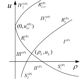
Figure 7.1.

1. For $\theta>0$, by [11], we have the following phase plane for fixed $(\rho_{L},u_{L})$ as shown in Fig. 7.1, on which $(0,u_{cr}^{(\theta)})$ with $u_{cr}^{(\theta)}=u_{L}+\frac{\rho_{L}^{\theta}}{\theta}$ is the intersect point of $R^{(\theta)}_{1}$ and $\{\rho=0\}$, and $R^{(\theta)}_{2,cr}$ is the $2$-rarefaction curve starting from $(0,u_{cr}^{(\theta)})$ separating region $IV_{2}^{(\theta)}$ from $IV_{1}^{(\theta)}$.

• If $(\rho_{R},u_{R})\in I^{(\theta)}$, then solution $(\rho^{(\theta)},u^{(\theta)})$ is $S^{(\theta)}_{1}+R^{(\theta)}_{2}$.

• If $(\rho_{R},u_{R})\in II^{(\theta)}$, then solution $(\rho^{(\theta)},u^{(\theta)})$ is $S^{(\theta)}_{1}+S^{(\theta)}_{2}$.

• If $(\rho_{R},u_{R})\in III^{(\theta)}$, then solution $(\rho^{(\theta)},u^{(\theta)})$ is $R^{(\theta)}_{1}+S^{(\theta)}_{2}$.

• If $(\rho_{R},u_{R})\in IV_{1}^{(\theta)}$, then solution $(\rho^{(\theta)},u^{(\theta)})$ is $R^{(\theta)}_{1}+R^{(\theta)}_{2}$ with the middle state $\rho_{M}^{(\theta)}>0$.

• If $(\rho_{R},u_{R})\in IV_{2}^{(\theta)}$, then solution $(\rho^{(\theta)},u^{(\theta)})$ is $R^{(\theta)}_{1}+R^{(\theta)}_{2}$ with the middle state $\rho_{M}^{(\theta)}=0$.

The criterion for the last case is $\rho_{M}^{\left(\theta\right)}=0$ if and only if $\xi_{1}^{(\theta)}:=u_{L}+\frac{\rho^{\theta}_{L}}{\theta}\leq u_{R}-\frac{\rho^{\theta}_{R}}{\theta}=:\xi_{2}^{(\theta)}$.

Figure 7.2.

2. For $\theta=0$, we have the following phase plane for fixed $(\rho_{L},u_{L})$ as shown in Fig. 7.2 similarly, on which $R^{(0)}_{1}$ and $\{\rho=0\}$ do not intersect.

• If $(\rho_{R},u_{R})\in I^{(0)}$, then solution $(\rho^{(0)},u^{(0)})$ is $S^{(0)}_{1}+R^{(0)}_{2}$.

• If $(\rho_{R},u_{R})\in II^{(0)}$, then solution $(\rho^{(0)},u^{(0)})$ is $S^{(0)}_{1}+S^{(0)}_{2}$.

• If $(\rho_{R},u_{R})\in III^{(0)}$, then solution $(\rho^{(0)},u^{(0)})$ is $R^{(0)}_{1}+S^{(0)}_{2}$.

• If $(\rho_{R},u_{R})\in IV^{(0)}$, then solution $(\rho^{(0)},u^{(0)})$ is $R^{(0)}_{1}+R^{(\theta)}_{2}$.

Then we have the existence and uniqueness of the Riemann solution $(\rho^{(\theta)},u^{(\theta)})$ for all $\theta\geq 0$.

3. For the shock curves, a direct computation yields that $(S^{(\theta)}_{1},S^{(\theta)}_{2})\rightarrow(S^{(0)}_{1},S^{(0)}_{2})$ and the shock speed $\sigma^{(\theta)}\rightarrow\sigma^{(0)}$ uniformly as $\theta\rightarrow 0$, since $\rho_{L}$ and $\rho_{R}>0$. Similar to the computation of (5.12), for the case that $\rho_{L}>0$ and $\rho_{R}>0$, $(R^{(\theta)}_{1},R^{(\theta)}_{2})\rightarrow(R^{(0)}_{1},R^{(0)}_{2})$ and

$$(\lambda^{(\theta)}_{1},\lambda^{(\theta)}_{2})=(u-\rho^{\theta},u+\rho^{\theta})\,\rightarrow\,(\lambda^{(0)}_{1},\lambda^{(0)}_{2})=(u-1,u+1)\qquad\mbox{uniformly as $\theta\rightarrow 0$}.$$

Thus, we conclude that the shock and rarefaction wave curves converge strongly, for the two-side non-vacuum case.

4. With the convergence of each wave curve, we turn to the convergence of the corresponding Riemann solutions $(\rho^{(\theta)},u^{(\theta)})$. The argument is divided into two cases:

Case 1: $\rho^{(\theta)}_{M}>0$ for all $\theta>0$. In this case, for the fixed left-state $(\rho_{L},u_{L})$, the right-state $(\rho_{R},u_{R})$ belongs to $\bigcap_{\theta\in(0,\theta_{0}]}\big{(}I^{(\theta)}\cup II^{(\theta)}\cup III^{(\theta)}\cup IV^{(\theta)}_{1}\big{)}$. The conclusion of Step 3 leads to the uniform convergence of $(\rho^{(\theta)},u^{(\theta)})\to(\rho^{(0)},u^{(0)})$ as $\theta\rightarrow 0$.

Case 2: There exists $\theta_{*}$ such that $\rho^{(\theta_{*})}_{M}=0$. For this case, $(\rho_{R},u_{R})\in IV_{2}^{(\theta_{*})}$, then solution $(\rho^{(\theta_{*})},u^{(\theta_{*})})$ is $R^{(\theta_{*})}_{1}+R^{(\theta_{*})}_{2}$ with $\xi_{1}^{(\theta_{*})}\leq\xi_{2}^{(\theta_{*})}$. Notice that

$$\xi_{2}^{(\theta)}-\xi_{1}^{(\theta)}=\big{(}u_{R}-\frac{\rho^{\theta}_{R}}{\theta}\big{)}-\big{(}u_{L}+\frac{\rho^{\theta}_{L}}{\theta}\big{)}=(u_{R}-u_{L})-\frac{\rho^{\theta}_{L}+\rho^{\theta}_{R}}{\theta}.$$

There exists $\underline{\theta}_{*}<\theta_{*}$ such that $\xi_{2}^{(\theta)}<\xi_{1}^{(\theta)}$ for $\theta<\underline{\theta}_{*}$, which leads to $\rho^{(\theta)}_{M}>0$. The rest of the argument is same as Case 1. ∎

Remark 7.1.

From Case $2$, we observe that the centered vacuum state with $\rho^{(\theta)}_{M}=0$ vanishes when $\theta$ is small enough. This represents the phenomenon of decavitation as $\gamma\to 1$, which is different from the formation of cavitation and concentration in the vanishing pressure limit $($equivalently, the high Mach limit$)$ in presented in Chen-Liu [8].

Next, we consider the one-side vacuum case. Without loss of generality, we assume that $\rho_{L}=0$, which connects $R^{(\theta)}_{2}$ with $R^{(0)}_{2}$. Notice that the fluid velocity $u_{L}$ is not well-defined in the vacuum with $\rho_{L}=0$ in general. In the following analysis, we fix the right-state $(\rho_{R},u_{R})$.

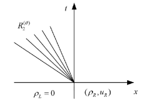
Figure 7.3.

For $\theta>0$, the Riemann solution $(\rho^{(\theta)},u^{(\theta)})$ as shown in Fig. 7.3 is

$$(\rho^{(\theta)},u^{(\theta)})=\begin{cases}((\frac{\theta\frac{x}{t}-\theta u_{L}+\rho_{R}^{\theta}}{\theta+1})^{\frac{1}{\theta}},\frac{\frac{x}{t}+\theta u_{L}-\rho_{R}^{\theta}}{\theta+1})\qquad\,&\mbox{for $u_{R}-\frac{\rho^{\theta}_{R}}{\theta}<\frac{x}{t}<u_{R}+\rho_{R}^{\theta}$},\\[2.84526pt] (\rho_{R},u_{R})\qquad\,&\mbox{for $\frac{x}{t}\geq u_{R}+\rho_{R}^{\theta}$},\end{cases}$$

and $\rho^{(\theta)}=0$ when $\frac{x}{t}\leq u_{R}-\frac{\rho^{\theta}_{R}}{\theta}$. Moreover, $u^{(\theta)}(t,x)=u_{R}-\frac{\rho^{\theta}_{R}}{\theta}$ at $\frac{x}{t}=u_{R}-\frac{\rho^{\theta}_{R}}{\theta}+0$.

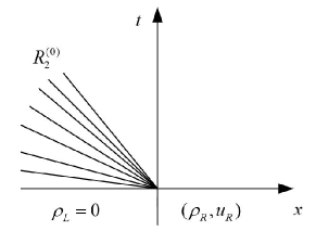
Figure 7.4.

For $\theta=0$, the Riemann solution $(\rho^{(0)},u^{(0)})$ as shown in Fig. 7.4 is

$$(\rho^{(0)},u^{(0)})=\begin{cases}(\rho_{L}e^{\frac{x}{t}-u_{L}-1},\frac{x}{t}-1)\qquad\,&\mbox{for $\frac{x}{t}<u_{R}+1$},\\[2.84526pt] (\rho_{R},u_{R})\qquad\,&\mbox{for $\frac{x}{t}\geq u_{R}+1$}.\end{cases}$$

Moreover, $u^{(0)}(t,x)\rightarrow-\infty$ as $\frac{x}{t}\rightarrow-\infty$.

For $\theta\rightarrow 0$, it is direct to see that $u_{R}-\frac{\rho^{\theta}_{R}}{\theta}\rightarrow-\infty$ and $u_{R}+\rho^{\theta}_{R}\rightarrow u_{R}+1$, which leads to $(\rho^{(\theta)},u^{(\theta)})\rightarrow(\rho^{(0)},u^{(0)})$.

Notice that

$$\lim_{\theta\rightarrow 0}\lim_{\frac{x}{t}\rightarrow u_{R}-\frac{\rho^{\theta}_{R}}{\theta}+0}c^{(\theta)}(\rho^{(\theta)}(t,x))=0,\qquad\lim_{\theta\rightarrow 0}c^{(\theta)}(\rho^{(\theta)}(t,x))\equiv 1,$$

which indicate the order of the limits on the sound speed $c^{(\theta)}$ close to the vacuum can not change in general.

The above case shows the convergence of the one-side vacuum states. However, $u_{L}$ is not well-defined in the vacuum with $\rho_{L}=0$, so that (2.18) is not well-defined as well.

Finally, we construct a family of Riemann solutions $(\rho^{(\theta)}_{A},u^{(\theta)}_{A})$ approaching $(\rho^{(0)},u^{(0)})$ with the initial data satisfying (2.18). Choose the initial data:

$$(\rho^{(\theta)}_{A},u^{(\theta)}_{A})(0,x)=\begin{cases}(\rho^{(\theta)}_{L},u^{(\theta)}_{L})\qquad\,&\mbox{for $x<0$},\\ (\rho_{R},u_{R})\qquad\,&\mbox{for $x>0$},\end{cases}$$

with $\rho^{(\theta)}_{L}=O(\theta^{\frac{1}{\theta}})$ and $u^{(\theta)}_{L}=u_{R}-\frac{\rho_{R}^{\theta}-(\rho^{(\theta)}_{L})^{\theta}}{\theta}$. It is direct to check that $(\rho^{(\theta)}_{A},u^{(\theta)}_{A})(0,x)$ satisfy (2.18).

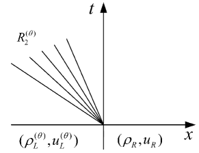
Figure 7.5.

Then the Riemann solutions $(\rho^{(\theta)}_{A},u^{(\theta)}_{A})$ as shown in Fig. 7.5 is

$$(\rho^{(\theta)}_{A},u^{(\theta)}_{A})=\begin{cases}(\rho^{(\theta)}_{L},u^{(\theta)}_{L})\qquad\,&\mbox{for $\frac{x}{t}\leq u^{(\theta)}_{L}+(\rho^{(\theta)}_{L})^{\theta}$},\\[2.84526pt] ((\frac{\theta\frac{x}{t}-\theta u_{L}+\rho_{R}^{\theta}}{\theta+1})^{\frac{1}{\theta}},\frac{\frac{x}{t}+\theta u_{L}-\rho_{R}^{\theta}}{\theta+1})\qquad\,&\mbox{for $u^{(\theta)}_{L}+(\rho^{(\theta)}_{L})^{\theta}<\frac{x}{t}<u_{R}+\rho_{R}^{\theta}$},\\[2.84526pt] (\rho_{R},u_{R})\qquad\,&\mbox{for $\frac{x}{t}\geq u_{R}+\rho_{R}^{\theta}$}.\end{cases}$$

When $\theta\rightarrow 0$, we see that $\rho^{(\theta)}_{L}\rightarrow 0$, $u^{(\theta)}_{L}\rightarrow-\infty$, $u^{(\theta)}_{L}+\big{(}\rho^{(\theta)}_{L}\big{)}^{\theta}\rightarrow-\infty$, and $u_{R}+\rho^{\theta}_{R}\rightarrow u_{R}+1$. Similarly, we conclude that $(\rho^{(\theta)}_{A},u^{(\theta)}_{A})\rightarrow(\rho^{(0)},u^{(0)})$.

Acknowledgments: The research of Gui-Qiang G. Chen was supported in part by the UK Engineering and Physical Sciences Research Council Awards EP/L015811/1, EP/V008854/1, and EP/V051121/1. The research of Fei-Min Huang was supported by the NSFC Grant No. 12288201. The research of Tian-Yi Wang was supported in part by the NSFC Grants 11971024 and 12061080.

References

- [1] J. Ball, A version of the fundamental theorem of Young measures, In: PDEs and Continuum Models of Phase Transitions, pp. 207–215, Lecture Notes of Physics, 344, Springer-Verlag, 1989.
- [2] G.-Q. Chen, Convergence of the Lax-Friedrichs scheme for isentropic gas dynamics (III), Acta Math. Sci. 6B (1986), 75–120 (in English); 8A (1988), 243–276 (in Chinese).
- [3] G.-Q. Chen, Vacuum states and global stability of rarefaction waves for compressible flow, Methods Appl. Anal. 7 (2000), 75–120.
- [4] G.-Q, Chen, C. Christoforou, and Y. Zhang, Dependence of entropy solutions in the large for the Euler equations on nonlinear flux functions, Indiana Univ. Math. J. 56 (2007), 2535–2568.
- [5] G.-Q. Chen, C. Christoforou, and Y. Zhang, Continuous dependence of entropy solutions to the Euler equations on the adiabatic exponent and Mach number, Arch. Ration. Mech. Anal. 189 (2008), 97–130.
- [6] G.-Q. Chen and P. LeFloch, Compressible Euler equations with general pressure law, Arch. Ration. Mech. Anal. 153 (2000), 221–259.
- [7] G.-Q. Chen and P. LeFloch, Existence theory for the isentropic Euler equations, Arch. Ration. Mech. Anal. 166 (2003), 81–98.
- [8] G.-Q. Chen and H. Liu, Formation of -shocks and vacuum states in the vanishing pressure limit of solutions to the Euler equations for isentropic fluids, SIAM J. Math. Anal. 34 (2003), 925–938.
- [9] G.-Q. Chen and M. Perepelitsa, Vanishing viscosity limit of the Navier-Stokes equations to the Euler equations for compressible fluid flow, Comm. Pure Appl. Math. 63(11) (2010), 1469–1504.
- [10] C. Christoforou, M. Galanopoulou, and A. E. Tzavaras, A symmetrizable extension of polyconvex thermoelasticity and applications to zero-viscosity limits and weak-strong uniqueness. Comm. Partial Diff. Equ. 43 (2018), 1019–1050.
- [11] C. M. Dafermos, Hyperbolic Conservation Laws in Continuum Physics, Springer-Verlag: Berlin, 2016.
- [12] X. Ding, G.-Q. Chen, and P. Luo, Convergence of the Lax-Friedrichs scheme for the isentropic gas dynamics (I)–(II), Acta Math. Sci. 5B (1985), 483–500, 501–540 (in English); 7A (1987), 467–480; 8A (1989), 61–94 (in Chinese).
- [13] X. Ding, G.-Q. Chen, and P. Luo, Convergence of the fractional step Lax-Friedrichs scheme and Godunov scheme for the isentropic system of gas dynamics, Commun. Math. Phys. 121 (1989), 63–84.
- [14] R. J. DiPerna, Convergence of the viscosity method for isentropic gas dynamics, Commun. Math. Phys. 91 (1983), 1–30.
- [15] L. C. Evans, Weak Convergence Methods for Nonlinear Partial Differential Equations, CBMS-RCSM, 74. AMS: Providence, RI, 1990.
- [16] F.-M. Huang and Z. Wang, Convergence of viscosity solutions for isothermal gas dynamics. SIAM J. Math. Anal. 34 (2002), 595–610.
- [17] P. LeFloch and V. Shelukhin, Symmetries and global solvability of the isothermal gas dynamics equations, arXiv Preprint arXiv:0701100, 2007.
- [18] P.-L. Lions, B. Perthame, and P. Souganidis, Existence and stability of entropy solutions for the hyperbolic systems of isentropic gas dynamics in Eulerian and Lagrangian coordinates, Comm. Pure Appl. Math. 49 (1996), 599–638.
- [19] P.-L. Lions, B. Perthame, and E. Tadmor, Kinetic formulation of the isentorpic gas dynamics and p-systems, Commun. Math. Phys. 163 (1994), 415–431.
- [20] F. Murat, Compacité par compensation, Ann. Scuola Norm. Sup. Pisa Sci. Fis. Mat. 5 (1978), 489–507.
- [21] T. Nishida, Global solution for an initial boundary value problem of a quasilinear hyperbolic system, Proc. Japan Acad. 44 (1968) 642–646.
- [22] T. Nishida and J. Smoller, Solutions in the large for some nonlinear hyperbolic conservation laws, Comm. Pure Appl. Math. 26 (1973), 183–200.
- [23] B. Perthame, Kinetic Formulation of Conservation Laws, Oxford University Press: Oxford, 2002.
- [24] M. R. Schrecker and S. Schulz, Vanishing viscosity limit of the compressible Navier-Stokes equations with general pressure law. SIAM J. Math. Anal. 51 (2019), 2168–2205.
- [25] L. Tartar, Compensated compactness and applications to partial differential equations, In: Research Notes in Mathematics, Nonlinear Analysis and Mechanics, Herriot-Watt Symposium, Vol. 4, R. J. Knops ed., Pitman Press, 1979.