Hyper-differential sensitivity analysis for nonlinear Bayesian inverse problems

Abstract

We consider hyper-differential sensitivity analysis (HDSA) of nonlinear Bayesian inverse problems governed by PDEs with infinite-dimensional parameters. In previous works, HDSA has been used to assess the sensitivity of the solution of deterministic inverse problems to additional model uncertainties and also different types of measurement data. In the present work, we extend HDSA to the class of Bayesian inverse problems governed by PDEs. The focus is on assessing the sensitivity of certain key quantities derived from the posterior distribution. Specifically, we focus on analyzing the sensitivity of the MAP point and the Bayes risk and make full use of the information embedded in the Bayesian inverse problem. After establishing our mathematical framework for HDSA of Bayesian inverse problems, we present a detailed computational approach for computing the proposed HDSA indices. We examine the effectiveness of the proposed approach on a model inverse problem governed by a PDE for heat conduction.

Keywords: Bayesian inverse problems, post optimality sensitivity analysis, model uncertainty, design of experiments.

1 Introduction

Many natural phenomena can be described by systems of partial differential equations (PDEs). The governing PDEs, however, often include parameters that are unknown and challenging to measure directly. This gives rise to inverse problems, in which one uses the PDE model and measurement data to estimate the unknown model parameters. In this article we consider Bayesian inverse problems [1, 2], whose solution is a posterior distribution that is informed by both our prior knowledge and the data measurements. Specifically, we focus on Bayesian inverse problems governed by PDEs with infinite-dimensional parameters.

In addition to the parameters being estimated, the governing PDEs typically contain parameters that are uncertain but needed for a full model specification. For clarity, we refer to the parameters being estimated by the inverse problem as inversion parameters and call the additional model parameters the auxiliary parameters. Another source of uncertainty in the inverse problem arises from the parameters specifying the experimental conditions, such as the location of measurement devices or their accuracy. We call these the experimental parameters. Throughout the article we will refer to the union of auxiliary and experimental parameters as complementary parameters. Our goal in this article is to develop methods for assessing the sensitivity of the solution of a Bayesian inverse problems with respect to perturbations of complementary parameters; see Section 2 for a simple illustrative example.

Understanding the sensitivity of an inverse problem to complementary parameters is important. These parameters may differ from their measured or estimated values, which in turn will result in a solution different from the one we would obtain if we had access to perfect measurements and true auxiliary parameters. Determining the sensitivity of the solution to perturbations in these parameters can inform our modeling assumptions and experimental design practices. Specifically, this can guide a goal oriented prioritization of resources and focus efforts on obtaining accurate values for the important auxiliary parameters. Moreover, if one has data that is informative to the important auxiliary parameters, the inverse problem may be redesigned to include these parameters in the set of inversion parameters.

The present work builds on previous efforts in hyper-differential sensitivity analysis (HDSA) [3, 4, 5, 6, 7, 8, 9, 10, 11, 12]. Traditional HDSA uses the derivative of the solution of an optimization problem with respect to complementary parameters to define sensitivity indices. These indices measure how much the solution of the optimization problem changes when the complementary parameters are perturbed. Specifically, in our previous work [3], which targets deterministic inverse problems, we define two types of sensitivity indices: pointwise sensitivities, and generalized sensitivities. Pointwise indices measure the sensitivity of the solution to perturbation in specific complementary parameters. Generalized indices measure the maximum possible change in the solution with respect to any unit perturbation of groups of complementary parameters. These indices provide a framework to study the sensitivity of the inverse problem solution; see [3] for more details.

In the present work, we extend HDSA to the class of Bayesian inverse problems, which allows us to study the change in the posterior distribution with respect to perturbations of the complementary parameters. We focus on HDSA of Bayesian inverse problems governed by PDEs with infinite-dimensional parameters. Section 3 provides a brief overview of the inverse problems under study. HDSA of a Bayesian inverse problem is difficult, because the solution of such problems is a statistical distribution. In general, the posterior distribution is difficult to approximate; this makes assessing the sensitivity of the posterior to complementary parameters challenging. A tractable approach is to instead focus on certain key aspects of the posterior distribution. Namely, we consider specific quantities of interest (QoIs) derived from the posterior distribution to perform HDSA on; we call such quantities the HDSA QoIs.

A first possibility, which we consider in this article, is to assess the sensitivity of the maximum a posteriori probability (MAP) point to the complementary parameters. This builds directly on the developments in [3]. Of greater difficulty is obtaining sensitivities of a measure of the posterior uncertainty. A natural setting for defining such measures is provided by the theory of optimal experimental design (OED) [13, 14, 15, 16, 17, 18]. Recall that in OED, one seeks experiments that minimize posterior uncertainty or, more generally, optimize the statistical quality of the estimated parameters. This is done by optimizing certain design criteria. Examples include the A-optimality criterion, which quantifies the average posterior variance, or the Bayesian D-optimality criterion, measuring the expected information gain; see e.g., [16]. In the present work, we consider the Bayes risk, which has been used previously in OED for PDE-constrained inverse problems [19, 20, 21]. Our motivations for using the Bayes risk as an HDSA QoI are two-fold. First, the Bayes risk is defined as an average error of the MAP estimator; see Section 4.1. Thus, HDSA of the Bayes risk builds further on methods for HDSA of the MAP point. Moreover, it is well-known [16, 22] that the Bayes risk, with respect to the $L^{2}$ loss function, reduces to the A-optimality criterion, in the case of Gaussian linear Bayesian inverse problem. Hence, up to a linearization, the Bayes risk may be considered as a proxy for the average posterior variance. Bayes risk is also a common utility function in decision theory.

The contributions of this article are as follows:

• We develop a mathematical framework to assess the sensitivity of the Bayes risk and the MAP point in nonlinear Bayesian inverse problems with respect to complementary parameters; see Section 4.

• We present a scalable computational framework for computing the HDSA indices for the MAP point and the Bayes risk; see Section 5. In that section, we also detail the computational cost of the various components of the proposed approach.

• We present comprehensive numerical results for a model problem of heat flow across a conductive surface that examine the effectiveness and efficiency of the proposed approach; see Section 6 for the description of the model under study and Section 7 for our computational results.

2 An Illustrative Example

We consider a simple example to motivate the problem considered in this work, which is to conduct sensitivity analysis on the solution of Bayesian inverse problems. Consider the heat equation,

$$\frac{\partial y(x,t)}{\partial t} =\exp(m)\frac{\partial^{2}y(x,t)}{\partial x^{2}}, x\in(0,\pi),t\in(0,1)$$ (1a)

$$y(0,t) =y(\pi,t)=0, t\in(0,1)$$ (1b)

$$y(x,0) =\sin(x)+\exp(\theta)\sin(2x), x\in(0,\pi).$$ (1c)

In this problem, $m$ is the inversion parameter and $\theta$ is an uncertain auxiliary parameter. For simplicity we let $m$ and $\theta$ be scalars here. Following a Bayesian framework, we endow $m$ with a Gaussian prior $m\sim\mathcal{N}(1.3,.1)$. The problem (1) can be solved analytically and the solution is given by,

$$y(x,t)=\exp(-\exp(m)t)\sin(x)+\exp(-4\theta\exp(m)t)\sin(2x).$$

We have collected data measurements with additive Gaussian noise at the final time $t=1$ at six evenly spaced points between $x=0$ and $x=\pi$ depicted in Figure 1. The Gaussian noise is unbiased with a standard deviation of 26 in this example. By Bayes rule, the posterior probability density function (pdf) is proportional to the product of the likelihood and prior pdfs. Because the auxiliary parameter is uncertain, we want to understand how the posterior distribution changes as the auxiliary parameter is perturbed. We view the posterior pdf of $m$ solved at the nominal value of $\theta=-.3$ and a perturbed value of $\theta=-.29$ in Figure 1.

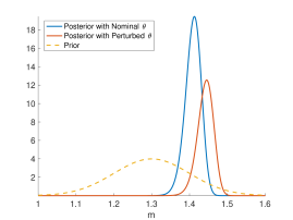
Figure 1: Left: the solution of the PDE at the final time with noisy data measurements, Right: the prior pdf of $m$ and its posterior pdf for both a nominal and perturbed value of the auxiliary parameter $\theta$.

We notice two primary changes in the posterior pdf as the auxiliary parameter is perturbed. First, there is a shift in the location of the distribution’s peak, which equates to a change in the MAP point. Second, there is a change in the spread or variance of the distribution which equates to a changing of the posterior uncertainty. We can see that perturbations of auxiliary parameters can have significant impact upon both of these posterior quantities.

3 Bayesian inverse problems and complementary parameters

We let $\boldsymbol{\theta}_{a}$ and $\boldsymbol{\theta}_{e}$ denote the auxiliary and experimental parameters, and call the augmented parameter vector $\boldsymbol{\theta}=\begin{bmatrix}\boldsymbol{\theta}_{a}\\ \boldsymbol{\theta}_{e}\end{bmatrix}$ the complementary parameters. Note that it is possible to have some auxiliary parameters that are functions (see [3]) but to keep the presentation simple, we consider finite-dimensional complementary parameters. The precise definition of the experimental parameters is, in general, application dependent, but in what follows we consider a particular case. Our goal is to provide a comprehensive framework for analyzing the sensitivity of the solution of the inverse problems under study to perturbations in $\boldsymbol{\theta}$.

We assume that the governing PDE (the state equation), represented abstractly by

$$v(u,m,\boldsymbol{\theta}_{a})=0,$$ (2)

has a unique solution $u$ for a given $m$ and fixed auxiliary parameters $\boldsymbol{\theta}_{a}$. The inversion parameter $m$ belongs to an infinite-dimensional Hilbert space $\mathcal{M}$ that is equipped with an inner product $\langle\cdot,\cdot\rangle_{\mathcal{M}}$ and the induced norm $\|\cdot\|_{\mathcal{M}}$. The state variable $u$ belongs to an infinite dimensional reflexive Banach space $U$. In the present work, $\mathcal{M}=L^{2}(\Omega)$ where $\Omega$ is a suitable physical domain and $\langle\cdot,\cdot\rangle_{\mathcal{M}}$ is the standard $L^{2}$ inner product.

To infer $m$, we solve a Bayesian inverse problem that uses observed measurements along with information known about the governing system of PDEs. We assume that (noisy) measurement data is related to $m$ according to the following model:

$$\boldsymbol{y}=\boldsymbol{F}(m,\boldsymbol{\theta}_{a})+\boldsymbol{\eta}(\boldsymbol{\theta}_{e}),$$ (3)

where $\boldsymbol{y}$ is a vector of $n_{y}$ experimental measurements, $\boldsymbol{F}$ the parameter-to-observable map that takes in the inversion parameter $m$ and maps it to a vector of measurements, and $\boldsymbol{\eta}$ a vector that models additive Gaussian noise, $\boldsymbol{\eta}\sim\mathcal{N}(\boldsymbol{0},\mathbf{{\Gamma}}_{\text{noise}}(\boldsymbol{\theta}_{e}))$. Evaluating $\boldsymbol{F}(m,\boldsymbol{\theta}_{a})$ requires solving the state equation (2) followed by application of an observation operator $\mathcal{O}$ which evaluates the state $u$ at the $n_{y}$ sensor locations. In the present work we let $\boldsymbol{\theta}_{e}$ parameterize the noise levels of the sensors. This can correspond to situations where the experimental error at various sensors can be controlled either by repeated measurements or by choice of the measurement device, or possibly recalibration of existing devices. Our model for the experimental parameters is detailed in Section 6.

The Bayesian inverse problem setup. To solve an inverse problem with the data model (3) we define the data likelihood pdf $\pi_{\text{like}}(\boldsymbol{y}|m;\boldsymbol{\theta})$, which describes the distribution of data measurements $\boldsymbol{y}$, given a particular inversion parameter $m$. Given our assumption of an additive Gaussian noise model, we have $\boldsymbol{y}|m\sim\mathcal{N}(\boldsymbol{F}(m),\mathbf{{\Gamma}}_{\text{noise}})$, and thus,

$$\pi_{\text{like}}(\boldsymbol{y}|m;\boldsymbol{\theta})\propto\exp\left(-\frac{1}{2}(\boldsymbol{F}(m,\boldsymbol{\theta}_{a})-\boldsymbol{y}(\boldsymbol{\theta}_{e}))^{\top}\mathbf{{\Gamma}}_{\text{noise}}^{-1}(\boldsymbol{\theta}_{e})(\boldsymbol{F}(m,\boldsymbol{\theta}_{a})-\boldsymbol{y}(\boldsymbol{\theta}_{e}))\right).$$ (4)

Note that in (4) the auxiliary parameters appear in the parameter-to-observable map $\boldsymbol{F}$ while we assume the experimental parameters for our problem appear only in the data measurements themselves and the noise covariance matrix.

In a Bayesian paradigm, we model our uncertainty regarding the inversion parameter by modeling $m$ as a random variable. Accordingly, we endow the inversion parameter $m$ with a prior distribution that reflects our knowledge of $m$ a priori. In the present work, we let the prior distribution law be a Gaussian $\mu_{\text{pr}}=\mathcal{N}(m_{\text{pr}},\mathcal{C}_{\text{pr}})$, with mean $m_{\text{pr}}$ and covariance operator $\mathcal{C}_{\text{pr}}$. We let $\mathcal{C}_{\text{pr}}=\mathcal{A}^{-2}$ where $\mathcal{A}$ is a Laplace-like differential operator; see, e.g.,[18, 2, 23]. The Gaussian prior measure is meaningful since $\mathcal{A}^{-2}$ is a trace class operator which guarantees bounded variance and almost surely pointwise well-defined samples. The prior measure induces the Cameron-Martin space $\mathscr{E}=\text{range}(\mathcal{C}_{\text{pr}}^{1/2})$, which is endowed with the following inner product,

$$\langle x,y\rangle_{\mathscr{E}}=\langle\mathcal{A}x,\mathcal{A}y\rangle.$$

We assume $m_{\text{pr}}\in\mathscr{E}$.

The definition of the prior measure and the data likelihood completes the description of the Bayesian inverse problem. The solution of this inverse problem is called the posterior measure $\mu_{\text{post}}^{\boldsymbol{y}}$, which describes the probability law of $m$ conditioned on experimental measurements $\boldsymbol{y}$. We will often denote the posterior measure as $\mu_{\text{post}}$ for notational simplicity when no confusion arises from doing so. The Bayes formula takes the following form in the infinite-dimensional Hilbert space setting [2]

$$\frac{d\mu_{\text{post}}}{d\mu_{\text{pr}}}\propto\pi_{\text{like}}(\boldsymbol{y}|m;\boldsymbol{\theta}).$$

Also, for a fixed $\boldsymbol{\theta}$, the maximum a posteriori probability (MAP) estimator of $m$ is found by solving

$$m^{*}(\boldsymbol{\theta})\coloneqq\underset{{m\in\mathscr{E}}}{\operatorname{argmin}}\ J(m,\boldsymbol{\theta}),$$ (5)

where

$$J(m,\boldsymbol{\theta})\coloneqq\frac{1}{2}\big{(}\boldsymbol{F}(m,\boldsymbol{\theta}_{a})-\boldsymbol{y}(\boldsymbol{\theta}_{e})\big{)}^{\top}\mathbf{{\Gamma}}_{\text{noise}}^{-1}(\boldsymbol{\theta}_{e})\big{(}\boldsymbol{F}(m,\boldsymbol{\theta}_{a})-\boldsymbol{y}(\boldsymbol{\theta}_{e})\big{)}+\frac{1}{2}\langle m-m_{\text{pr}},m-m_{\text{pr}}\rangle_{\mathscr{E}}.$$ (6)

Discretization. In the present work, we follow a continuous Galerkin finite element discretization and let $\boldsymbol{m}$ and $\boldsymbol{u}$ be the discretizations of their continuous counterparts $m$ and $u$. We let $n_{m}$ be the the dimension of the discretized parameter. The discretized space is $\mathbb{R}^{n_{m}}$ equipped with the inner product

$$\langle{\boldsymbol{a}},{\boldsymbol{b}}\rangle_{\mathbf{{M}}}=\boldsymbol{a}^{\top}\mathbf{{M}}\boldsymbol{b},\quad\boldsymbol{a},\boldsymbol{b}\in\mathbb{R}^{n_{m}},$$

where $\mathbf{{M}}$ is the finite element mass matrix, and the norm $\|\cdot\|_{\mathbf{{M}}}$ induced by this inner product. Note that when working with linear operators on $(\mathbb{R}^{n_{m}},\|\cdot\|_{\mathbf{{M}}})$ or linear transformations between $(\mathbb{R}^{n},\|\cdot\|_{\mathbf{{M}}})$ and $(\mathbb{R}^{n},\|\cdot\|)$, where $\|\cdot\|$ is the Euclidean inner product, the adjoint operators need to be defined appropriately; see [23] for this and further details on discretization of different components of infinite-dimensional Bayesian inverse problems. In the remainder of this article, we present the proposed methods in the discretized setting.

4 HDSA for Nonlinear Bayesian Inverse Problems

In this section, we outline a framework for HDSA of nonlinear Bayesian inverse problems.

4.1 The HDSA QoIs

As discussed in the introduction, we consider two HDSA QoIs for a Bayesian inverse problem: (i) the MAP point, which is obtained by minimizing (6) and (ii) the Bayes risk. The Bayes risk, for a fixed vector $\boldsymbol{\theta}$ of complementary parameters, is defined by

$$\Psi_{\text{risk}}(\boldsymbol{\theta})=\int_{\mathcal{M}}\int_{\mathbb{R}^{d}}\|\boldsymbol{m}^{*}(\boldsymbol{\theta})-\boldsymbol{m}\|_{\mathbf{{M}}}^{2}\pi_{\text{like}}(\boldsymbol{y}|\boldsymbol{m};\boldsymbol{\theta})d\boldsymbol{y}\mu_{\text{pr}}^{n_{m}}(d\boldsymbol{m}).$$ (7)

Note that here we expressed the Bayes risk for the discretized version of the Bayesian inverse problem, and $\boldsymbol{m}^{*}$ is the discretized MAP point. The discretized prior measure, which we denote by $\mu_{\text{pr}}^{n_{m}}$ should be defined appropriately, as described in [23].

In practice, Bayes Risk is approximated via sample averaging. Namely, we draw $n_{s}$ samples $\{\boldsymbol{m}_{1},\dots,\boldsymbol{m}_{n_{s}}\}$ from the prior distribution to compute data samples $\{\boldsymbol{y}_{1},\dots,\boldsymbol{y}_{n_{s}}\}$ with the forward data model,

$$\boldsymbol{y_{i}}=\boldsymbol{F}(\boldsymbol{m}_{i},\boldsymbol{\theta}_{a})+\boldsymbol{\eta}_{i}(\boldsymbol{\theta}_{e}),\qquad i=1,\dots,n_{s},$$

where $\boldsymbol{\eta}_{i}$ are sample draws from noise distribution $\mathcal{N}(0,\mathbf{{\Gamma}}_{\text{noise}}(\boldsymbol{\theta}_{e}))$. We can then rewrite the approximate Bayes Risk as

$$\widehat{\Psi}_{\text{risk}}(\boldsymbol{\theta})=\frac{1}{n_{s}}\sum_{i=1}^{n_{s}}\|\boldsymbol{m}^{*}(\boldsymbol{y}_{i},\boldsymbol{\theta})-\boldsymbol{m}_{i}\|_{\mathcal{M}}^{2}.$$ (8)

4.2 Sensitivity operator of Bayes risk

To compute the sensitivity operator of the approximate Bayes risk estimator, we first discretize (8) and denote its discretization by $\widehat{\mathbf{{\Psi}}}_{\text{risk}}(\boldsymbol{\theta})$. We assess the sensitivity of Bayes risk by differentiating $\widehat{\mathbf{{\Psi}}}_{\text{risk}}(\boldsymbol{\theta})$ with respect to $\theta_{j}$, the $j^{\text{th}}$ component of $\boldsymbol{\theta}$, and evaluate at a set of nominal complementary parameter values $\boldsymbol{\theta}^{*}$:

$$D^{\text{R}}_{j}\coloneqq\frac{\partial}{\partial\theta_{j}}\widehat{\mathbf{{\Psi}}}_{\text{risk}}(\boldsymbol{\theta}^{*})=\frac{2}{n_{s}}\sum_{i=1}^{n_{s}}\frac{\partial}{\partial\theta_{j}}(\boldsymbol{m}^{*}(\boldsymbol{y}_{i},\boldsymbol{\theta}^{*}))^{\top}\mathbf{{M}}\boldsymbol{m}^{*}(\boldsymbol{y}_{i},\boldsymbol{\theta}^{*})-\frac{\partial}{\partial\theta_{j}}(\boldsymbol{m}^{*}(\boldsymbol{y}_{i},\boldsymbol{\theta}^{*}))^{\top}\mathbf{{M}}\boldsymbol{m}_{i}.$$

We define the discretized sensitivity operator of the approximate Bayes risk as

$$\mathbf{{D}}^{\text{R}}=\begin{bmatrix}D^{\text{R}}_{1}&D^{\text{R}}_{2}&\dots&D^{\text{R}}_{n_{\theta}}\end{bmatrix},$$ (9)

where $n_{\theta}$ denotes the dimension of the complementary parameter vector. Note that $\mathbf{{D}}^{\text{R}}\tilde{\boldsymbol{\theta}}$ can be interpreted as the sensitivity of the approximate Bayes risk with respect to a perturbation of the complementary parameters in the direction $\tilde{\boldsymbol{\theta}}$.

To compute the derivative of the approximate Bayes risk, we need $\frac{\partial\boldsymbol{m}^{*}}{\partial\theta}(\boldsymbol{y}_{i},\boldsymbol{\theta}^{*})$, $i=1,\ldots,n_{s}$, which measures the sensitivity of the MAP points (for each data sample $\boldsymbol{y}_{i}$) to the complementary parameters . For clarity, we denote the discretized cost functional by $\boldsymbol{J}$. As discussed in [3], under mild regularity assumptions [4, 5, 24] using the implicit function theorem, we obtain

$$\mathbf{{D}}^{\text{M}}=\frac{\partial\boldsymbol{m}^{*}}{\partial\boldsymbol{\theta}}=-\left(\frac{\partial^{2}\boldsymbol{J}}{\partial\boldsymbol{m}^{2}}\right)^{-1}\frac{\partial^{2}\boldsymbol{J}}{\partial\boldsymbol{m}\partial\boldsymbol{\theta}}=-\mathbf{{H}}^{-1}\mathbf{{B}},$$ (10)

where $\mathbf{{H}}$ and $\mathbf{{B}}$ are evaluated at the solution $\boldsymbol{m}^{*}$ with fixed nominal parameters $\boldsymbol{\theta}^{*}$. By averaging these computed sensitivities over the number of data samples $n_{s}$, we can simultaneously measure both the average MAP point and Bayes risk sensitivities.

It is important to note the significance of this process. In a deterministic formulation  [3], the sensitivities of the inverse problem solution $\boldsymbol{m}^{*}$ require data measurements to compute. That is, some experimental measurements would be needed before conducting sensitivity analysis. In contrast, the method proposed here does not require experimental measurements and can be computed a priori by using the information encoded in the Bayesian inverse problem to generate likely data realizations. This makes the methodology applicable to a broad range of problems where data is not available at the time of performing HDSA.

4.3 Sensitivity Indices

Given a sensitivity operator, we define sensitivity indices to provide a scalar which measures the magnitude of the change in the solution with respect to a particular perturbation of the complementary parameters. We first group related complementary parameters together into $K$ subsets. For example, we group data measurements corresponding to the same state variable together, scalar auxiliary parameters form their own group (of size 1), while all parameters defining the discretization of an uncertain function may form another group. Let $\Theta_{k}$ be the inner product space containing the $k$th set of parameters for $k=1,\dots,K$ and $\{\boldsymbol{b}_{k}^{1},\boldsymbol{b}_{k}^{2},\dots,\boldsymbol{b}_{k}^{n_{k}}\}$ be a basis for $\Theta_{k}$ of dimension $n_{k}$. We then define $\{\boldsymbol{e}_{k}^{j}\}$ as the basis of $\Theta=\Theta_{1}\times\Theta_{2}\times\dots\times\Theta_{K}$ for $k=1,\dots,K$ and $j=1,\dots,n_{k}$ where

$$\boldsymbol{e}_{k}^{j}=\begin{pmatrix}\boldsymbol{0}_{1}&\dots&\boldsymbol{0}_{k-1}&\boldsymbol{b}_{k}^{j}&\boldsymbol{0}_{k+1}&\dots&\boldsymbol{0}_{K}\end{pmatrix}^{\top}.$$

We can now define pointwise sensitivity indices to measure the sensitivity of both the MAP point and the approximate Bayes risk as,

$$S_{k}^{j}=\frac{\|\mathbf{{D}}^{\text{M}}\boldsymbol{e}_{k}^{j}\|_{\mathbf{{M}}}}{\|\boldsymbol{e}_{k}^{j}\|_{\Theta}}\qquad\text{and}\qquad\mathbb{S}_{k}^{j}=\frac{|\mathbf{{D}}^{\text{R}}\boldsymbol{e}_{k}^{j}|}{\|\boldsymbol{e}_{k}^{j}\|_{\Theta}}$$ (11)

respectively. These pointwise sensitivities measure the change in the MAP point or Bayes risk, respectively, to a perturbation of the $k$th parameter in the $j$th direction $\boldsymbol{b}_{k}^{j}$.

We would also like to determine the importance of the $K$ parameter subgroups relative to one another. To do so, we define generalized sensitivity indices which provide a single measure of sensitivity for each parameter subgroup. Let $\mathbf{{T}}_{k}:\Theta\to\Theta$ be a selection operator that zeros out components of $\boldsymbol{\theta}$ not in $\Theta_{k}$. We define the generalized sensitivity of the $k$th subgroup of complementary parameters with respect to the MAP point and approximate Bayes risk respectively as,

$$S_{k}=\max_{\boldsymbol{\theta}\in\Theta}\frac{\|\mathbf{{D}}^{\text{M}}\mathbf{{T}}_{k}\boldsymbol{\theta}\|_{\mathbf{{M}}}}{\|\boldsymbol{\theta}\|_{\Theta}}\qquad\text{and}\qquad\mathbb{S}_{k}=\max_{\boldsymbol{\theta}\in\Theta}\frac{|\mathbf{{D}}^{\text{R}}\mathbf{{T}}_{k}\boldsymbol{\theta}|}{\|\boldsymbol{\theta}\|_{\Theta}}.$$ (12)

The generalized sensitivities measure the maximum change that can be observed in the HDSA QoIs to a norm-1 perturbation of the $k$th parameter subgroup. We can interpret this as a “worst case scenario” sensitivity because it measures the maximum change in the solution. More importantly, the generalized sensitivities provide a single measure of sensitivity for each parameter subgroup which can be used to compare their relative importance, despite their potentially diverse range of physical characteristics. Note that the parameter groupings should be specified by the user and are problem dependent. In the model problem considered in Section 6 we allow scalar auxiliary parameters to each consist of their own subgroup while the experimental parameters, corresponding to noise in the data measurements, are grouped together. It is important to note that if a subgroup consists of a single scalar parameter, its pointwise and generalized sensitivities will be identical. We direct the reader to [3] for additional details on the construction of these sensitivities.

To compare the MAP point and Bayes risk sensitivities it is important to note that each sensitivity is endowed with specific units. If we were only concerned with a single HDSA QoI, this would not matter because we would be primarily concerned with the relative differences between sensitivities of that measure. When comparing the sensitivities of the MAP point to Bayes risk however, we must normalize with respect to the QoI to compare the sensitivities to each other in a reasonable fashion. To do so, we divide the sensitivities with respect to the MAP point by the average norm of the computed MAP points, $\frac{1}{n_{s}}\sum_{i=1}^{n_{s}}\|\boldsymbol{m}^{*}(\boldsymbol{y}_{i},\boldsymbol{\theta}^{*})\|_{\mathbf{{M}}}$, and the sensitivities with respect to Bayes risk by the computed value of Bayes risk, $\widehat{\mathbf{{\Psi}}}_{\text{risk}}(\boldsymbol{\theta}^{*})$.

5 Computational Methods

In this section, we present computational methods to implement the framework proposed in Section 4.

5.1 Computing the sensitivity indices

With the discretization of $\boldsymbol{m}$ and its prior, we can write the sensitivity operator of the approximate Bayes risk with respect to the complementary parameters (9) as,

$$\mathbf{{D}}^{\text{R}}=\frac{2}{n_{s}}\sum_{i=1}^{n_{s}}(\mathbf{{D}}^{\text{M}_{i}})^{\top}\mathbf{{M}}\left(\boldsymbol{m}^{*}(\boldsymbol{y}_{i},\boldsymbol{\theta}^{*})-\boldsymbol{m}_{i}\right)=\frac{2}{n_{s}}\sum_{i=1}^{n_{s}}-\mathbf{{B}}_{i}^{\top}\mathbf{{H}}_{i}^{-\top}\mathbf{{M}}\left(\boldsymbol{m}^{*}(\boldsymbol{y}_{i},\boldsymbol{\theta}^{*})-\boldsymbol{m}_{i}\right).$$ (13)

We let the subscript $i$ on the operators $\mathbf{{D}}^{\text{M}_{i}}\in\mathbb{R}^{n_{m}\times n_{\theta}}$, $\mathbf{{B}}_{i}\in\mathbb{R}^{n_{m}\times n_{\theta}}$, and $\mathbf{{H}}_{i}\in\mathbb{R}^{n_{m}\times n_{m}}$ indicate the dependence on the $i$th data sample.

To compute matrix-free actions of $\mathbf{{H}}$ and $\mathbf{{B}}$ to vectors, we use a discretized formal Lagrangian approach. We note that this method is utilized to both compute sensitivity indices as well as solve for the MAP point. We begin by defining the discrete Lagrangian as

$$\mathcal{L}(\boldsymbol{u},\boldsymbol{m},\boldsymbol{p};\boldsymbol{\theta})=\boldsymbol{J}(\boldsymbol{m},\boldsymbol{\theta})-\langle{\boldsymbol{p}},{\boldsymbol{v}(\boldsymbol{u},\boldsymbol{m},\boldsymbol{\theta}_{a})}\rangle_{\mathbf{{M}}}$$ (14)

where $\boldsymbol{v}(\boldsymbol{u},\boldsymbol{m},\boldsymbol{\theta}_{a})$ is the discretized form of the PDE $v$, and $\boldsymbol{p}$ is the adjoint variable. Next, we use variational derivatives to compute the action of the discretized gradient of the cost function. We let $\mathcal{L}_{\boldsymbol{p}}[\hat{\boldsymbol{p}}]$ denote the variational derivative of (14) with respect to $\boldsymbol{p}$, acting on $\hat{\boldsymbol{p}}$, with the input arguments suppressed for brevity. A similar notation is used for the variational derivatives with respect to $\boldsymbol{u}$ and $\boldsymbol{m}$. We can also compute the action of the Hessian by constructing a meta-Lagrangian,

$$\mathcal{L}^{H}(\boldsymbol{u},\boldsymbol{m},\boldsymbol{p},\hat{\boldsymbol{u}},\hat{\boldsymbol{m}},\hat{\boldsymbol{p}};\boldsymbol{\theta})=\mathcal{L}_{\boldsymbol{p}}[\hat{\boldsymbol{p}}]+\mathcal{L}_{\boldsymbol{u}}[\hat{\boldsymbol{u}}]+\mathcal{L}_{\boldsymbol{m}}[\hat{\boldsymbol{m}}].$$ (15)

By computing variational derivatives of the meta-Lagrangian, we can evaluate the action of the discretized Hessian to vectors. The basic steps of this solution process are outlined in Algorithm 1, and we direct the reader to [25, 26] for additional details.

Algorithm 1 Compute the gradient g($\boldsymbol{m}$) and action of the Hessian $\mathbf{{H}}$ in the direction $\hat{\boldsymbol{m}}$

1:  Solve the state equation $\mathcal{L}_{\boldsymbol{p}}=0\quad$ for the state variable $\boldsymbol{u}$

2:  Solve the adjoint equation $\mathcal{L}_{\boldsymbol{u}}=0\quad$ for the adjoint variable $\boldsymbol{p}$

3:  Evaluate $g(\boldsymbol{m})^{\top}=\mathcal{L}_{\boldsymbol{m}}$

4:  Solve the incremental state equation $\mathcal{L}^{H}_{\boldsymbol{p}}=0\quad$ for the incremental state variable $\hat{\boldsymbol{u}}$

5:  Solve the incremental adjoint equation $\mathcal{L}^{H}_{\boldsymbol{u}}=0\quad$ for the incremental adjoint variable $\hat{\boldsymbol{p}}$

6:  Evaluate the Hessian apply $\mathbf{{H}}(\boldsymbol{m})[\hat{\boldsymbol{m}}]=\mathcal{L}^{H}_{\boldsymbol{m}}$

Next, we discuss computing the action of the mixed derivative operator $\mathbf{{B}}^{\top}$. We follow a similar approach as one used to compute the action of the Hessian using the meta-Lagrangian $\mathcal{L}^{H}$. Namely, we differentiate the mata-Lagrangian with respect to $\boldsymbol{\theta}$ to obtain

$$\mathcal{L}^{H}_{\boldsymbol{\theta}}(\boldsymbol{u},\boldsymbol{m},\boldsymbol{p},\hat{\boldsymbol{u}},\hat{\boldsymbol{m}},\hat{\boldsymbol{p}};\boldsymbol{\theta})[\tilde{\boldsymbol{\theta}}]=\tilde{\boldsymbol{\theta}}^{\top}\mathbf{{B}}^{\top}\hat{\boldsymbol{m}},$$

where $\hat{\boldsymbol{u}}$ and $\hat{\boldsymbol{p}}$ satisfy the incremenal state and and adjoint equations, respectively.

Note that we can also compute the action of $\mathbf{{B}}$ by reversing the order of differentiation, deriving through the Lagrangian by $\boldsymbol{\theta}$ and the meta-Lagrangian by $\boldsymbol{m}$, which will result in modified incremental equations. These adjoint based methods provide a computationally efficient method to evaluate the sensitivity operators $\mathbf{{D}}^{\text{M}}$ and $\mathbf{{D}}^{\text{R}}$.

To compute the discretized sensitivity operator $\mathbf{{D}}^{\text{R}}$, we must first generate data samples $\boldsymbol{y}_{i}$ for $i=1,\dots,n_{s}$ and then evaluate (13) which requires non-trivial computational cost. We also compute sensitivities of the MAP point, efficiently reusing PDE solves whenever applicable. This process is summarized in Algorithm 2. Note that for clarity, we have separated the processes of data generation and sensitivity operator computation in the algorithm. Furthermore, in Algorithm 2 the second subscript in sensitivity indices $S_{k,i}$ denotes dependence of the index upon the $i$th data sample.

Algorithm 2 Compute the sensitivity indices

1:  % Data sample generation

2:  for $i=1$ to $n_{s}$ do

3:     Draw prior sample $\boldsymbol{m}_{i}$

4:     Solve the forward equation $\boldsymbol{v}(\boldsymbol{u}_{i},\boldsymbol{m}_{i},\boldsymbol{\theta}^{*}_{a})=\boldsymbol{0}$ for $\boldsymbol{u}_{i}$

5:     Synthesize data samples $\boldsymbol{y}_{i}=\mathcal{O}\boldsymbol{u}_{i}+\boldsymbol{\eta}_{i}(\boldsymbol{\theta}^{*}_{e})$ {$\mathcal{O}$ observes $\boldsymbol{u}$ at measurement locations}

6:  end for

7:  % Computation of the Bayes risk sensitivities

8:  for $i=1$ to $n_{s}$ do

9:     Solve the discretized inverse problem for $\boldsymbol{m}_{i}^{*}(\boldsymbol{d}_{i},\boldsymbol{\theta}^{*})$

10:     Solve $-\mathbf{{H}}_{i}\boldsymbol{z}_{i}=\mathbf{{M}}(\boldsymbol{m}_{i}^{*}-\boldsymbol{m}_{i})$ for $\boldsymbol{z}_{i}$

11:     Compute $\boldsymbol{r}_{i}=\mathbf{{B}}_{i}^{\top}\boldsymbol{z}_{i}$

12:  end for

13:  $\mathbf{{D}}^{\text{R}}$ = $\frac{2}{n_{s}}$$\sum_{i=1}^{n_{s}}\boldsymbol{r}_{i}$

14:  Compute $\mathbb{S}_{k}$ and $\mathbb{S}_{k}^{j}$ for all $k=1,\dots,K$ and $j=1,\dots,n_{\theta}$, see (11)

15:  % Computation of the average MAP point sensitivities

16:  for $i=1$ to $n_{s}$ do

17:     Compute $S_{k,i}$ for $k=1,\dots,K$

18:     for $j=1$ to $n_{\theta}$ do

19:        Compute $S_{k,i}^{j}$ for $k=1,\dots,K$

20:     end for

21:  end for

22:  Compute averaged generalized sensitivities $S_{k}\approx\bar{S}_{k}=\frac{1}{n_{s}}\sum_{i=1}^{n_{s}}S_{k,i}$, see (12)

23:  Compute averaged pointwise sensitivities $S_{k}^{j}\approx\bar{S}_{k}^{j}=\frac{1}{n_{s}}\sum_{i=1}^{n_{s}}S_{k,i}^{j}$, see (12)

5.2 Computational Costs

Here we discuss the areas of high computational cost in Algorithm 2. To gain computational efficiency, we rely on some key tools from PDE-constrained optimization: inexact Newton-CG for MAP estimation, adjoint methods gradient and Hessian computation, and low-rank approximations for efficient computation of inverse Hessian applies [23, 27, 28, 29]. In particular, by combining methods that make maximum use of the problem structure, we ensure that the computational complexity of our approach, in the terms of the number of PDEs solves, does not scale with the dimension of the discretized inversion parameter.

Generate data samples. We solve the forward problem $n_{s}$ times and use the resulting solutions to generate data.

MAP point solves. We solve the inverse problem $n_{s}$ times (line 9) using an inexact Newton conjugate gradient line search algorithm with Armijo backtracking. Each Newton step requires 2 PDE solves to compute the gradient and an additional $2I$ PDE solves to compute the Hessian apply where $I$ is the number of iterations required by the CG solver to find an appropriate search direction. Thus the total cost is $2L+2LI$ PDE solves where $L$ is the number of Newton steps taken. This cost in PDE solves multiplied by the number of samples $n_{s}$ becomes quite significant. However, since the samples drawn from the prior are independent of each other, these computations can be performed in parallel. We also note that we initialize the MAP point solves with the prior samples used to generate data samples.

Evaluating inverse Hessian applies. We now address the problem of repeated application of the inverse Hessian, which is required to compute both Bayes risk and MAP point sensitivities in lines 10, 17, and 19. We note that if one only wishes to compute Bayes risk sensitivities, this will not require repeated use of the same Hessian inverse, and line 10 can be evaluated with PCG. Assuming that MAP point sensitivities are also desired, we can offset this cost by computing a low-rank approximation with the Lancoz method to apply the Hessian inverse efficiently, as detailed in [23]. After computing this low-rank approximation, application of the Hessian inverse can be approximated by matrix-vector products. The computational cost of the Lanczos method is $2r+2$ PDE solves, where $r$ is the rank of the desired approximation.

Computing Bayes risk sensitivities. The sensitivity operator of Bayes risk is a vector, so we built this operator directly before computing indices. We begin this discussion by noting that we can solve the state and adjoint equations around the MAP point once for each data sample, and reuse these solves for each Hessian $\mathbf{{H}}_{i}$ and mixed derivative operator $\mathbf{{B}}_{i}$ or $\mathbf{{B}}^{\top}_{i}$ apply. Each Hessian apply requires 2 additional PDE solves (in addition to the forward and adjoint solves) for the incremental state and incremental adjoint equations. These incremental equation solves can be reused to compute the application of $\mathbf{{B}}^{\top}_{i}$, while $\mathbf{{B}}_{i}$ apply requires 2 more PDE solves for the modified incremental equations.

Computing MAP point sensitivities. The greatest computational cost in estimating the MAP point sensitivities comes in the repeated application of $\mathbf{{D}}^{\text{M}}$ to standard basis vectors $\boldsymbol{e}_{i}$ (line 19) to compute $n_{\theta}$ pointwise sensitivity indices for all $n_{s}$ data samples. As mentioned previously, this cost is significantly reduced by pre-computing a low-rank approximation that allows for fast Hessian inverse applications. It is also important to note that we reuse the inverse problem solves from computing the Bayes risk sensitivities in computing the MAP point sensitivities and we do not require any additional inverse problem solves here. Due to these various computational savings, we can estimate the MAP point sensitivities through sample averaging at a significantly reduced cost.

Table 1: Computational costs summary

Computation	Significant Cost per Sample ($n_{s}$)
Data Generation	1 PDE solve
Inverse Problem Solves	$2L+2LI$ PDE solves for $L$ Newton steps
	and $I$ PCG iterations
Hessian Inverse Approximation	$2r+2$ PDE solves where $r$ is the rank of
	the desired approximation
Bayes risk sensitivities	2 PDE solves
MAP point sensitivities	$2n_{\theta}$ PDE solves

The discussed computational costs are summarized in Table 1 for clarity. We remark that for the problem considered in the present work $n_{\theta}$ is not very large. For problems with a large number of complementary parameters, computing a suitable low-rank approximation of $\mathbf{{B}}$ may be helpful to reduce the cost of computing many MAP point sensitivities. We plan to investigate this in our future work.

6 Model Problem

In this section, we present a model inverse problem, involving heat flow across a conductive surface, that will be used to study our HDSA framework. We begin by describing the forward problem in Section 6.1 followed by the setup of the Bayesian inverse problem in Section 6.2.

6.1 Forward Model

Consider the problem of infering the log-conductivity field of a medium from measurements of temperature. Focusing on a cross section, we consider the problem in two space dimensions. The forward problem is governed by the following elliptic PDE, modeling steady state heat conduction on a unit square domain $\Omega$ with boundary $\partial\Omega=\cup_{i=1}^{4}\Gamma_{i}$, where $\Gamma_{1}$, $\Gamma_{2}$, $\Gamma_{3}$, and $\Gamma_{4}$ denote the bottom, right, top, and left edges of $\Omega$ respectively,

$$-\nabla\cdot(e^{m}\nabla u) =f \qquad\text{in }\Omega,$$ (16a)

$$e^{m}\nabla u\cdot n =0 \qquad\text{on }\Gamma_{1}\cup\Gamma_{3},$$ (16b)

$$e^{m}\nabla u\cdot n =\beta(T_{\text{amb}}-u) \qquad\text{on }\Gamma_{2},$$ (16c)

$$e^{m}\nabla u\cdot n =s \qquad\text{on }\Gamma_{4}.$$ (16d)

In this model, the inversion parameter $m(\boldsymbol{x})$ is a function representing the log of the heat conductivity of the non-homogeneous two-dimensional surface. We let $u(\boldsymbol{x})$ denote the temperature, $f(\boldsymbol{x})$ the heat source in the domain, $\beta$ the heat transfer coefficient of the medium, $T_{\text{amb}}$ the ambient temperature of the medium, and $s(x_{2})$ a boundary heat source function representing heat entering the domain from the left boundary. In this model problem, the equations in (16) are dimensionless and we let $T_{\text{amb}}=22$ and consider the heat transfer coefficient $\beta$ to be an uncertain auxiliary parameter with a nominal value of $\beta=1$.

The boundary heat source $s(x_{2})$ is modeled as follows,

$$s(x_{2})=s_{1}\exp\left(-\left(\frac{x_{2}-s_{3}}{s_{2}}\right)^{2}\right)$$

with auxiliary parameters $s_{1},s_{2},\text{and }s_{3}$ fixed at nominal values $s_{1}=30,s_{2}=.1,\text{and }s_{3}=.65$. The auxiliary parameters consist of the amplitude, spread, and location of the boundary heat source respectively. The heat source in the domain $f(\boldsymbol{x})$ is modeled as,

$$f(\boldsymbol{x})=f_{1}\exp\left[-\frac{1}{2}(\boldsymbol{x}-\boldsymbol{w})^{\top}\mathbf{{C}}_{1}(\boldsymbol{x}-\boldsymbol{w})\right]+f_{2}\exp\left[-\frac{1}{2}(\boldsymbol{x}-\boldsymbol{z})^{\top}\mathbf{{C}}_{2}(\boldsymbol{x}-\boldsymbol{z})\right],\quad\text{with}$$

$$\mathbf{{C}}_{1}=\begin{bmatrix}\frac{\cos^{2}(\gamma_{1})}{\sigma_{x_{1}}^{2}}+\frac{\sin^{2}(\gamma_{1})}{\sigma_{x_{2}}^{2}}&\frac{\sin(2\gamma_{1})}{2\sigma_{x_{2}}^{2}}-\frac{\sin(2\gamma_{1})}{2\sigma_{x_{1}}^{2}}\\ \frac{\sin(2\gamma_{1})}{2\sigma_{x_{2}}^{2}}-\frac{\sin(2\gamma_{1})}{2\sigma_{x_{1}}^{2}}&\frac{\sin^{2}(\gamma_{1})}{\sigma_{x_{1}}^{2}}+\frac{\cos^{2}(\gamma_{1})}{\sigma_{x_{2}}^{2}}\end{bmatrix}\text{ and }\mathbf{{C}}_{2}=\begin{bmatrix}\frac{\cos^{2}(\gamma_{2})}{\sigma_{x_{1}}^{2}}+\frac{\sin^{2}(\gamma_{2})}{\sigma_{x_{2}}^{2}}&\frac{\sin(2\gamma_{2})}{2\sigma_{x_{2}}^{2}}-\frac{\sin(2\gamma_{2})}{2\sigma_{x_{1}}^{2}}\\ \frac{\sin(2\gamma_{2})}{2\sigma_{x_{2}}^{2}}-\frac{\sin(2\gamma_{2})}{2\sigma_{x_{1}}^{2}}&\frac{\sin^{2}(\gamma_{2})}{\sigma_{x_{1}}^{2}}+\frac{\cos^{2}(\gamma_{2})}{\sigma_{x_{2}}^{2}}\end{bmatrix}.$$

In this formulation, $f_{1}$ and $f_{2}$ control the amplitude of the heat sources, $\boldsymbol{w}$ and $\boldsymbol{z}$ control the centers of the two sources, $\gamma_{1}$ and $\gamma_{2}$ their respective tilt angles, and $\sigma_{x_{1}}$ and $\sigma_{x_{2}}$ the spread of the heat sources in the $x_{1}$ and $x_{2}$ directions respectively. For this problem we fix these parameters at the following nominal values: $f_{1}=100,f_{2}=105,\boldsymbol{w}=(.8,.25),\boldsymbol{z}=(.5,.8),\gamma_{1}=-\pi/4,\gamma_{2}=.15,\sigma_{x_{1}}=.8,\sigma_{x_{2}}=.1$. We consider the amplitude, center point, and angle of each bar to be uncertain and thus let $f_{1},f_{5},w_{1},w_{2},z_{1},z_{2},\gamma_{1},$ and $\gamma_{2}$ be the auxiliary parameters for the right hand side heat source $f(\boldsymbol{x})$. Figure 2 depicts this heat source in the domain.

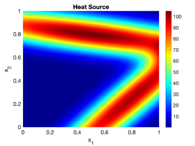
Figure 2: The heat source function $f(\boldsymbol{x})$

We note that this model problem has been kept intentionally simple to aid in the interpretation and understanding of the complicated algorithmic methodology. Even so, this example is motivated by many uncertainties surrounding additive manufacturing processes (such as powered bed laser fusion) that cause high residual stresses and even defects in final parts. Variability in the powder material, boundary conditions, rasterization patterns, and laser power result in uneven heat distribution with problematic micro-crystallographic structures and inhomogeneous material properties. Although the underlying physics for additive manufacturing is more complicated, our model problem conceptually demonstrates the ability of our approach to provide insight into a complicated application area.

6.2 Prior Measure and State Solution

In many inverse problems a “true solution” is chosen to synthesize data and evaluate the accuracy of the proposed methodology. Note that we do not have any such “true solution” here and instead we compute data from samples of the prior distribution. We specify the Bayesian prior on $m$ as a Gaussian random field on $\Omega$ with mean $m_{pr}$ and covariance operator $\mathcal{C}_{\text{pr}}$. We model the prior mean as a sinusoidal function:

$$m_{pr}(\boldsymbol{x})=1.5\sin(2\pi x_{1})\cos(2\pi x_{2})+2.$$

We let the covariance operator $\mathcal{C}_{\text{pr}}$ be the inverse of a squared elliptic differential operator $\mathcal{A}$, where $m=\mathcal{A}^{-1}s$ satisfies

$$\alpha\int_{\Omega}(\Phi\nabla m)\cdot\nabla q+mq\ d\boldsymbol{x}=\int_{\Omega}sq\ d\boldsymbol{x}$$

for all $q\in H^{1}(\Omega)$, with $\alpha=5$, and $\Phi=.01$. This formulation of the prior covariance ensures that $\mathcal{C}_{\text{pr}}$ is trace class and provides a computationally convenient formulation. For more details see [23].

Measurements are collected on an evenly spaced 5$\times$5 grid of observation locations depicted in Figure 3. We consider the standard deviation of the noise in each data measurement to be our uncertain experimental parameters. Additive Gaussian noise models “error” in our data and we assume the measurements are uncorrelated, with nominal standard deviations of $\sigma=.1$, thus $\mathbf{{\mathbf{{\Gamma}}_{\text{noise}}}}=\sigma^{2}\mathbf{{I}}$. Although we allow the measurement standard deviations to take the same nominal value, we consider each standard deviation individually when computing sensitivities of the solution. Perturbing the noise standard deviation will also result in a perturbation of the noise realization $\eta_{i}\sim\mathcal{N}(0,\mathbf{{\Gamma}}_{\text{noise}})$, directly proportional to the multiplicative perturbation of $\sigma_{i}$. Therefore the experimental parameters $\boldsymbol{\theta}_{e}$ enter the inverse problem through the cost function (6), both in the noise covariance matrix $\mathbf{{\Gamma}}_{\text{noise}}(\boldsymbol{\theta}_{e})$ and the data measurements $y(\boldsymbol{\theta}_{e})$ which depend on the noise realizations.

The solution of the governing PDE system detailed in (16) at the nominal parameter values with $m$ fixed at the prior mean is depicted in Figure 3.

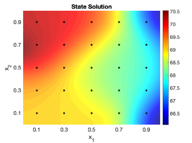
Figure 3: The state solution of the governing system of partial differential equations with the experimental sensor locations indicated by filled black circles.

7 Results

Using the model of heat flow across a conductive surface from Section 6, we solve an inverse problem to estimate the posterior distribution. Following Algorithm 2 to evaluate our Bayesian hyper-differential sensitivities, we take samples from the prior distribution on $m$ and push them through the forward mapping to generate noisy data. Each data sample is then used to solve (5), giving a unique MAP point reconstruction for each sample. To illustrate this process, we present three prior samples and their corresponding MAP point reconstructions in Figure 4.

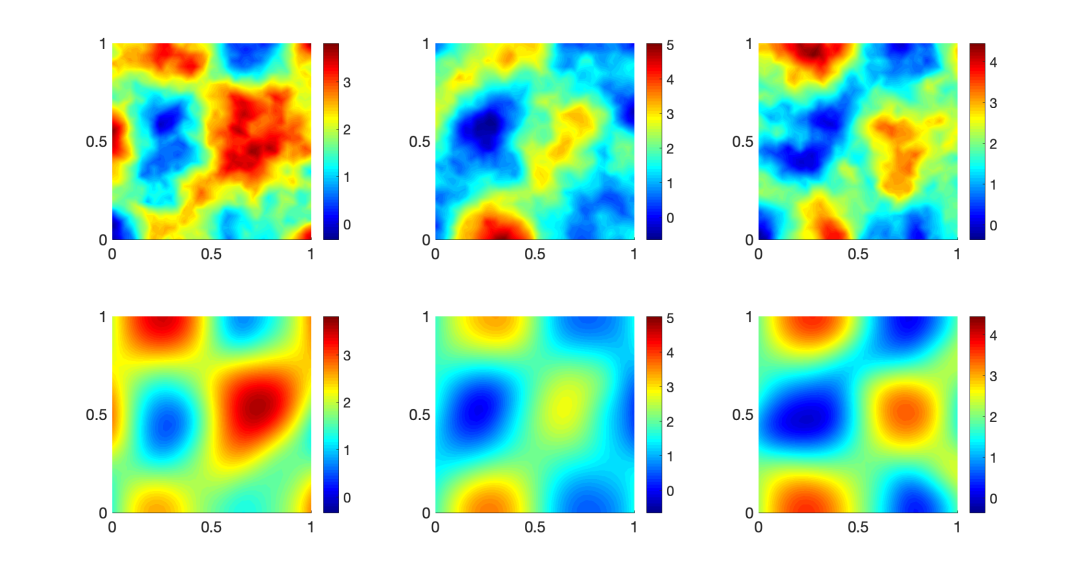
Figure 4: Top: three samples from the log-conductivity prior. Bottom: inverse problem MAP point estimates solved using data generated by the above prior sample.

Each MAP point is attempting to estimate the above prior sample from noisy data. This example is illustrative in that it gives us some insight into Bayes risk, which measures the average difference in norm between the prior samples (top) and the inferred MAP points (bottom).

In Section 7.1 we detail how perturbations of the complementary parameters are modeled. Following this we present and discuss the significance of the generalized sensitivities of the complementary parameters as well as the pointwise sensitivities of the experimental parameters with respect to Bayes risk (Section 7.2) and the MAP point (Section 7.3). We note that the pointwise sensitivities of the auxiliary parameters are identical to their generalized sensitivities as each auxiliary parameter is scalar valued in this model problem.

7.1 Modeling Parameter Perturbations

Suppose $\rho$ is an uncertain scalar parameter. We model our uncertainty in $\rho$ as,

$$\rho=\tilde{\rho}(1+a\theta)$$ (17)

where $\tilde{\rho}$ is the nominal value, $a$ is a scaling coefficient quantifying our degree of uncertainty, and $\theta\in[-1,1]$ defines a perturbation of $\tilde{\rho}$. Perturbations of vector valued complementary parameters, such as data measurements, are modeled as componentwise scalar perturbations as in (17).

In this particular model problem we use a perturbation scaling coefficient of $a=.05$ for each auxiliary parameter, which represents our uncertainty in that parameter’s estimate being $5\%$ of the parameter’s nominal value. For the experimental parameters we instead use a scaling coefficient of $a=1$ to represent that our uncertainty in the standard deviation of the data noise is the full quantity of the standard deviation.

7.2 Sensitivities of Bayes Risk

The approximate Bayes risk is computed as a sample average as detailed in (8). We present the generalized sensitivities of each complementary parameter with respect to Bayes risk in Figure 5. We study the effect of the sample size on the computed sensitivities by comparing generalized sensitivities for Bayes risk computed from ten groups of 20 samples, ten groups of 100 samples, and ten groups of 500 samples, each taken randomly from a group of 3000 pre-computed samples.

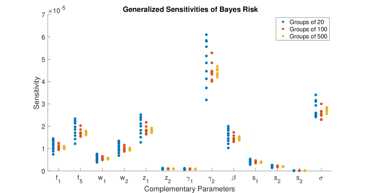
Figure 5: Generalized sensitivities of Bayes Risk to complementary parameters computed for 10 groups of samples of size 20, 100, and 500.

First let us discuss the spread of the samples. We can see that while the groups of 100 samples can sometimes vary significantly, such as in the case of $\gamma_{2}$, they generally capture the rankings of the parameters relative to one another correctly. Thus, if we are primarily concerned with determining the relative importance of the parameters compared to each other we may conclude that 100 samples provides sensitivity estimates that suit our needs.

Next, we note that Bayes risk is most sensitive to the tilt angle of the second domain heat source $\gamma_{2}$. We observe that as the tilt angles $\gamma_{1}$ and $\gamma_{2}$ are changed, they can overlap in the domain interior, causing a large increase in heat where the overlap occurs and will result a significant change in $f$. One possible reason $\gamma_{2}$ is so important is that even a relatively small perturbation will result in increased or decreased overlap of these bars in the domain. Of secondary importance are the heat amplitude ($f_{5}$) and center in the $x_{1}$ direction ($z_{1}$) of the second domain heat source, heat transfer coefficient ($\beta$), and the standard deviations of data noise ($\boldsymbol{\sigma}$). This sensitivity information can then be used by an experimenter to inform their experimental design choices for this problem. To accurately estimate the Bayes risk for this problem as a measure of posterior uncertainty, it is more important to invest resources in ensuring that the parameters $\gamma_{2},f_{5},z_{1},\beta$, and $\boldsymbol{\sigma}$ are accurately estimated than the other complementary parameters. Specifically, we can interpret these sensitivities as “a 5% perturbation in the scalar auxiliary parameters or a norm-1 perturbation in the experimental parameters ($\boldsymbol{\sigma}$) will result in a perturbation of Bayes risk proportional to the sensitivity.”

While these sensitivities appear to be very small, we note that the problem is highly diffusive and steady state. Both of these factors are likely making the problem highly insensitive to perturbations of complementary parameters. This in of itself showcases the benefits of using HDSA. For such an insensitive problem, it would be extremely difficult to gather any kind of intuition or conclusion as to the relative importance of various parameters a priori. With our framework however, we can rigorously determine the relative importance of uncertain parameters before any physical experimentation is done, even for highly insensitive problems, which is valuable to experimenters who seek to efficiently allocate experimental resources.

Next we study the pointwise sensitivities of Bayes risk to the experimental parameters, the standard deviation of noise in the data measurements, presented in Figure 6. By perturbing the noise, we model perturbations of each collected data measurement in a way that we can experimentally control through sensor accuracy.

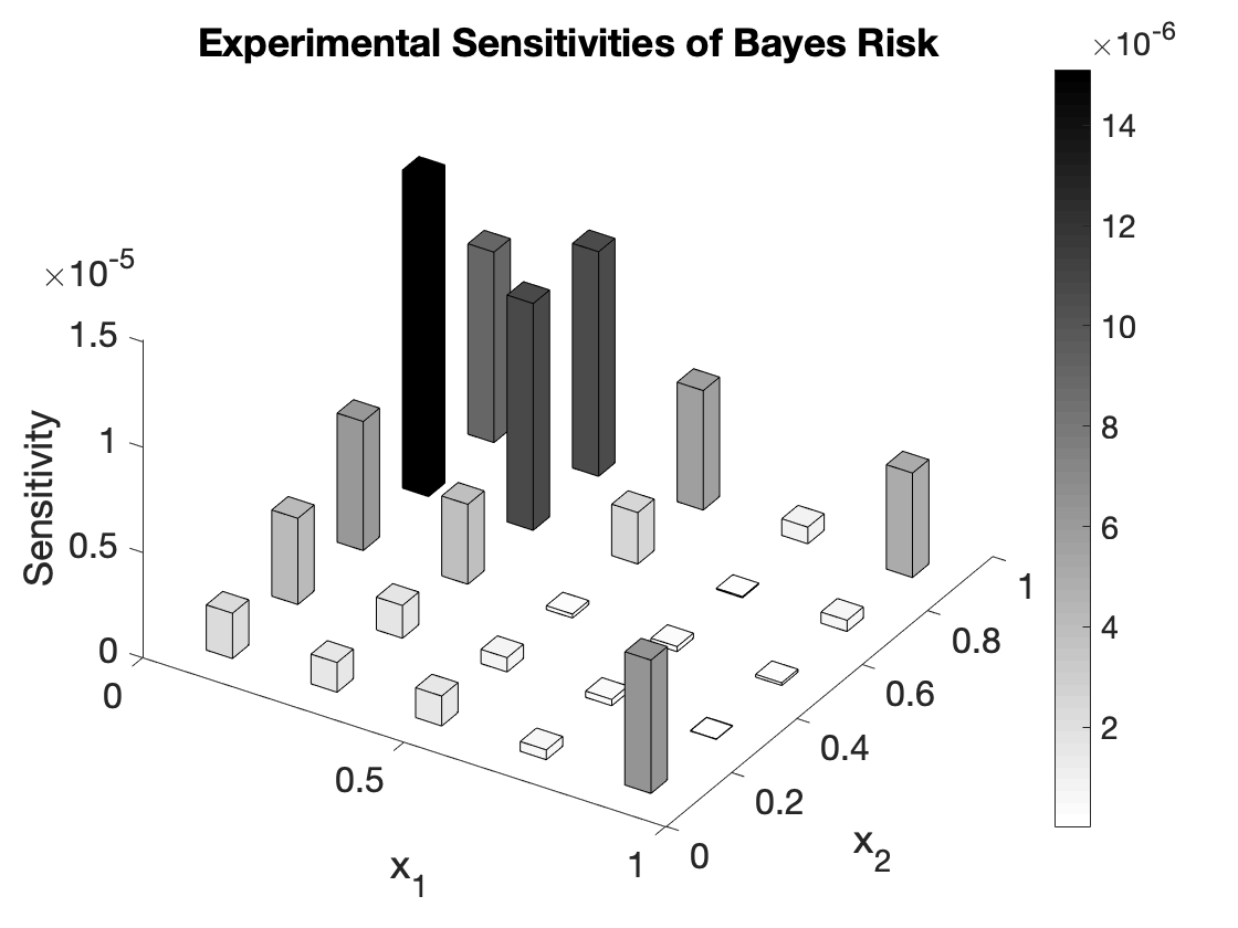
Figure 6: Point-wise sensitivities of Bayes Risk to experimental parameters computed from 1000 samples. Each bar represents the sensitivity of perturbing the standard deviation of the data noise at that particular sensor location.

We first note the scale of sensitivities presented in Figure 6. Although these sensitivities are very small (on the order of $10^{-5}$ or $10^{-6}$), this is not entirely unexpected given the scale of the generalized sensitivities presented in Figure 5. Indeed, we would expect that perturbing a single data measurement’s noise would not result in a very large change in Bayes risk. We can see that the sensors grouped around small values of $x_{1}$ and large values of $x_{2}$ are most important with respect to Bayes risk. Thus, we can conclude that the data measured at these sensors is the most important to collect accurately for the purposes of estimating our measure of posterior uncertainty. We observe that these sensors are located in the region that the state solution depicted in Figure 3 is largest. This is also the region near the boundary source term $s$. We also note that the sensors at (.9,.1) and (.9,.9) are relatively important, which are located in the areas where the state solution is smallest. These results provide information that may not be obvious a priori and helps practitioners understand what parameters and sensor measurements the solution is most sensitive to.

7.3 Sensitivities of the MAP Point

We now study the averaged generalized sensitivities of the MAP point. As was done previously, we study the effect of the sample size on the generalized sensitivities. This is done by computing generalized MAP point sensitivities for 3000 data samples. We then randomly select and average ten groups of 20 sensitivities, ten groups of 100 sensitivities, and ten groups of 500 sensitivities, which are plotted in Figure 7.

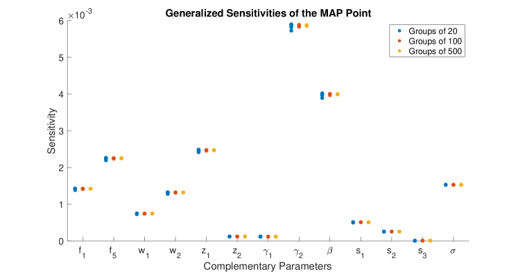
Figure 7: Averaged generalized sensitivities of the MAP point to complementary parameters computed for 10 groups of sensitivities of size 20, 100, and 500.

In this case we can see that even groups of 20 sensitivities produce little variation in the averaged sensitivity measure. Thus, we can conclude that for this application, using a sample average of just 20 sensitivities provides sufficient accuracy for our purposes. Furthermore, we notice that the generalized sensitivities of the MAP point are significantly greater in magnitude than those computed for Bayes risk. For this problem, it appears that the MAP point is more sensitive to perturbations in the complementary parameters than the posterior uncertainty is. We see that the MAP point has greatest sensitivity to $\gamma_{2},\beta,z_{1}$, and $f_{5}$. It is interesting to note that for Bayes risk, $\boldsymbol{\sigma}$ and $\beta$ had the second and fifth greatest sensitivity, respectively. In contrast, the sensitivity rankings of these two parameters have switched places with respect to the MAP point.

Finally, we examine the pointwise sensitivities of the MAP point to the experimental parameters depicted in Figure 8. Each pointwise sensitivity is computed as an average of 20 sensitivities computed from different data samples. We compared these pointwise sensitivities with those computed from an average of 1000 sensitivities, and as our study on sample size in Figure 7 would indicate, there was minimal difference.

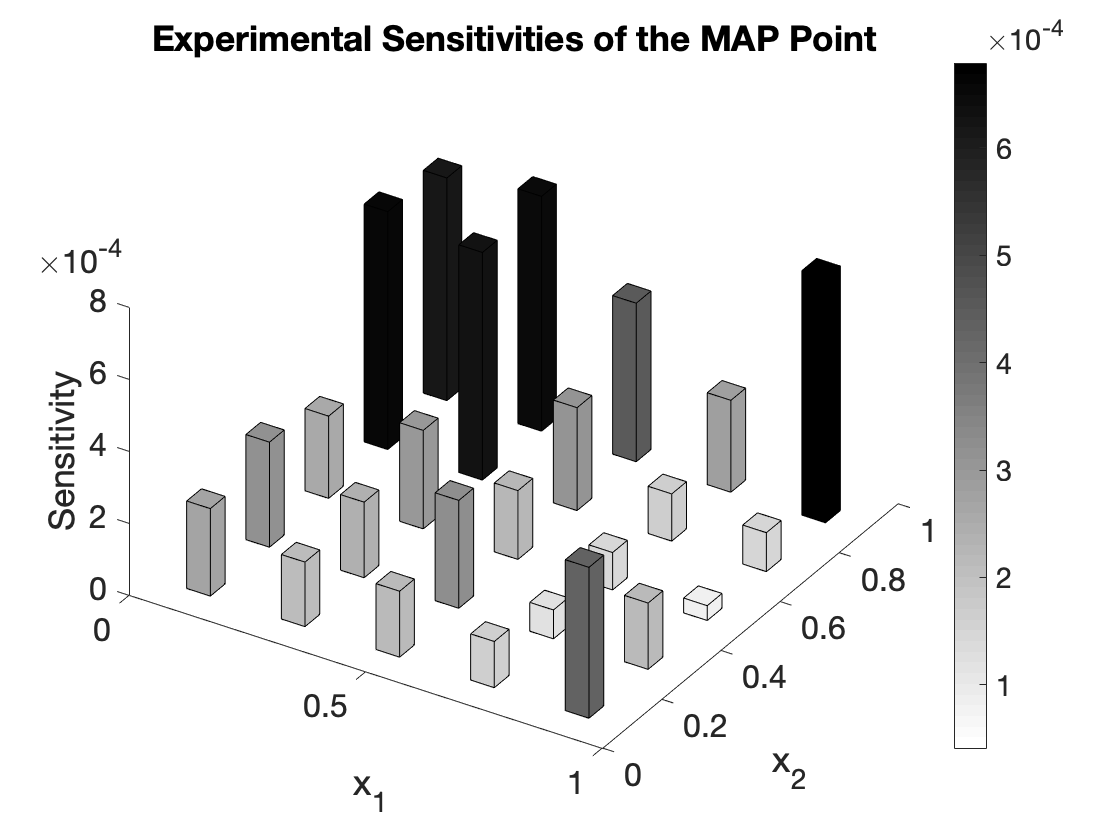
Figure 8: Point-wise sensitivities of the MAP point to experimental parameters computed as an average of 20 sample sensitivities.

We can again see that the sensors grouped around small values of $x_{1}$ and large values of $x_{2}$ are most important with respect to the MAP point. We observe that for this problem the sensors with greatest importance to the MAP point coincide closely with those sensors that are important for Bayes risk.

8 Conclusion

In this article we take foundational steps in applying hyper-differential sensitivity analysis (HDSA) to large-scale nonlinear Bayesian inverse problems. In particular, we focus on HDSA of the MAP point and Bayes risk to the auxiliary and experimental parameters and present efficient methods for computing the corresponding HDSA indices. Performing HDSA is important as it reveals the auxiliary parameters the inverse problem is most sensitive to. Moreover, HDSA with respect to measurement data helps identify the measurements that are important to the solution of the inverse problem, and can guide design of experiments by investing resources to obtain good quality data from important measurement points.

It is also important to note that the Bayesian formulation allows for the computation of HDSA indices prior to conducting experiments. Namely, we use the information encoded in the Bayesian inverse problem to obtain likely realizations of measurement data, which are used to compute the Bayes risk sensitivities and average MAP point sensitivities. This is a key factor that makes this approach attractive for HDSA of Bayesian inverse problems, while minimizing experimental costs.

While the steady state heat conduction model presented in Section 6 is an academic model problem, it has many features that are seen in real applications. We found that the tilt angle, heat amplitude, and center in the horizontal direction of volume heat source as well as the heat transfer coefficient and data noise were the parameters that both the Bayes risk and the MAP point were most sensitive to. We also determined which sensors provide the most informative data and found that for this problem the Bayes risk is generally less sensitive to perturbations of the complementary parameters than the MAP point is. Such observations can be instrumental in areas such as additive manufacturing. By applying the proposed methods to additive manufacturing problems, one can determine a priori which experimental factors the inverse problem solution will be most sensitive to and thereby guide the calibration of equipment tolerances with this information.

The MAP point is a key point estimator for the inversion parameters and performing HDSA on this quantity provides valuable insight regarding the sensitivity of the inverse problem to complementary parameters. On the other hand, Bayes risk provides a measure of the statistical quality of the estimated parameters, and is a common utility function in decision theory. Additionally, up to a linearization, Bayes risk can be considered as a proxy for posterior uncertainty. These considerations, coupled with the fact that the methods for HDSA of Bayes risk build on methods for HDSA of MAP point, made Bayes risk a suitable HDSA QoI in first steps towards HDSA of Bayesian inverse problems.

In our future work, we plan to investigate HDSA of different quantities such as average posterior variance or expected information gain. Suitable approximations of the posterior, such as a Laplace approximation, can be considered, to mitigate the high cost of HDSA of such quantities in large-scale nonlinear inverse problems. Another interesting line of inquiry is to use HDSA within the context of optimal experimental design (OED) under uncertainty [30, 31]. HDSA can reveal model uncertainties that the OED criterion is most sensitive to and thus must be accounted for in the optimal design process. On the other hand, model uncertainties the design criterion is less sensitive to may be fixed at some nominal values, hence reducing the complexity of OED under uncertainty problem.

Bibliography

Bibliography

- [1] Albert Tarantola. Inverse Problem Theory and Methods for Model Parameter Estimation. Society for Industrial and Applied Mathematics, 2005.
- [2] A M. Stuart. Inverse problems: A Bayesian perspective. Acta Numerica, 19:451–559, 05 2010.
- [3] Isaac Sunseri, Joseph Hart, Bart van Bloemen Waanders, and Alen Alexanderian. Hyper-differential sensitivity analysis for inverse problems constrained by partial differential equations. Inverse Problems, 36(12):125001, 2020.
- [4] Joseph Hart, Bart van Bloemen Waanders, and Roland Herzog. Hyper-differential sensitivity analysis of uncertain parameters in PDE-constrained optimization. International Journal for Uncertainty Quantification, 10(3):225–248, 2020.
- [5] Kerstin Brandes and Roland Griesse. Quantitative stability analysis of optimal solutions in PDE-constrained optimization. Journal of Computational and Applied Mathematics, 2006.
- [6] Roland Griesse and Andrea Walther. Parametric sensitivities for optimal control problems using automatic differentiation. Optimal Control Applications and Methods, 24:297–314, 2003.
- [7] Roland Griesse and Boris Vexler. Numerical sensitivity analysis for the quantity of interest in PDE-Constrained optimization. SIAM Journal on Scientific Computing, 29(1):22–48, 2007.
- [8] Roland Griesse. Stability and sensitivity analysis in optimal control of partial differential equations. Habilitation Thesis, Faculty of Natural Sciences, Karl-Franzens University, 2007.
- [9] Roland Griesse. Parametric sensitivity analysis in optimal control of a reaction diffusion system. I. solution differentiability. Numerical Functional Analysis and Optimization, 25(1-2):93–117, 2004.
- [10] Roland Griesse. Parametric sensitivity analysis in optimal control of a reaction-diffusion system – part II: practical methods and examples. Optimization Methods and Software, 19(2):217–242, 2004.
- [11] C. Büskens and R. Griesse. Parametric sensitivity analysis of perturbed PDE optimal control problems with state and control constraints. Journal of Optimization Theory and Applications, 131(1):17–35, 2006.
- [12] R. Griesse and S. Volkwein. Parametric sensitivity analysis for optimal boundary control of a 3D reaction-difusion system. In G. Di Pillo and M. Roma, editors, Nonconvex Optimization and its Applications, volume 83. Springer, Berlin, 2006.
- [13] A. C. Atkinson and A. N. Donev. Optimum Experimental Designs. Oxford, 1992.
- [14] A. Pázman. Foundations of Optimum Experimental Designs. D. Reidel Publishing Co., 1986.
- [15] F. Pukelsheim. Optimal Design of Experiments. John Wiley & Sons, New-York, 1993.
- [16] K. Chaloner and I. Verdinelli. Bayesian experimental design: A review. Statistical Science, 10(3):273–304, 1995.
- [17] Dariusz Uciński. Optimal Measurement Methods for Distributed Parameter System Identification. CRC Press, Boca Raton, 2005.
- [18] Alen Alexanderian. Optimal experimental design for infinite-dimensional bayesian inverse problems governed by pdes: a review. Inverse Problems, 2021.
- [19] Eldad Haber, Lior Horesh, and Luis Tenorio. Numerical methods for experimental design of large-scale linear ill-posed inverse problems. Inverse Problems, 24(055012):125–137, 2008.
- [20] Eldad Haber, Lior Horesh, and Luis Tenorio. Numerical methods for the design of large-scale nonlinear discrete ill-posed inverse problems. Inverse Problems, 26(2):025002, 2010.
- [21] Lior Horesh, Eldad Haber, and Luis Tenorio. Optimal Experimental Design for the Large-Scale Nonlinear Ill-Posed Problem of Impedance Imaging, pages 273–290. Wiley, 2010.
- [22] Alen Alexanderian, Philip J. Gloor, and Omar Ghattas. On Bayesian A- and D-Optimal Experimental Designs in Infinite Dimensions. Bayesian Analysis, 11(3):671–695, 2016.
- [23] Tan Bui-Thanh, Omar Ghattas, James Martin, and Georg Stadler. A computational framework for infinite-dimensional Bayesian inverse problems Part I: The linearized case, with application to global seismic inversion. SIAM Journal on Scientific Computing, 35(6):A2494–A2523, 2013.
- [24] Antonio Ambrosetti and Giovanni Prodi. A Primer of Nonlinear Analysis. Cambridge University Press, 1995.
- [25] Umberto Villa, Noemi Petra, and Omar Ghattas. hippylib: An extensible software framework for large-scale inverse problems governed by pdes: Part i: Deterministic inversion and linearized bayesian inference. ACM Transactions on Mathematical Software (TOMS), 47(2):1–34, 2021.
- [26] Max D. Gunzburger. Perspectives in Flow Control and Optimization. SIAM, 2003.
- [27] Noemi Petra, James Martin, Georg Stadler, and Omar Ghattas. A computational framework for infinite-dimensional bayesian inverse problems, part ii: Stochastic newton mcmc with application to ice sheet flow inverse problems. SIAM Journal on Scientific Computing, 36(4):A1525–A1555, 2014.
- [28] H Pearl Flath, Lucas C Wilcox, Volkan Akçelik, Judith Hill, Bart van Bloemen Waanders, and Omar Ghattas. Fast algorithms for bayesian uncertainty quantification in large-scale linear inverse problems based on low-rank partial hessian approximations. SIAM Journal on Scientific Computing, 33(1):407–432, 2011.
- [29] James Martin, Lucas C Wilcox, Carsten Burstedde, and Omar Ghattas. A stochastic newton mcmc method for large-scale statistical inverse problems with application to seismic inversion. SIAM Journal on Scientific Computing, 34(3):A1460–A1487, 2012.
- [30] Alen Alexanderian, Noemi Petra, Georg Stadler, and Isaac Sunseri. Optimal design of large-scale bayesian linear inverse problems under reducible model uncertainty: good to know what you don’t know. SIAM/ASA Journal on Uncertainty Quantification, 9(1):163–184, 2021.
- [31] Karina Koval, Alen Alexanderian, and Georg Stadler. Optimal experimental design under irreducible uncertainty for inverse problems governed by PDEs. Submitted, 2019. https://arxiv.org/abs/1912.08915.