The Generalized Fibonacci Oscillator as an Open Quantum System

The Generalized Fibonacci Oscillator
as an Open Quantum System

Franco FAGNOLA ^a, Chul Ki KO ^b and Hyun Jae YOO ^c

F. Fagnola, C.K. Ko and H.J. Yoo

^a) Mathematics Department, Politecnico di Milano, Piazza L. da Vinci 32, I-20133 Milano, Italy franco.fagnola@polimi.it https://www.mate.polimi.it/qp/

^b) University College, Yonsei University, 85 Songdogwahak-ro, Yeonsu-gu, Incheon 21983, Korea kochulki@yonsei.ac.kr

^c) School of Computer Engineering and Applied Mathematics,
^c) Institute for Integrated Mathematical Sciences, Hankyong National University,
^c) 327 Jungang-ro, Anseong-si, Gyeonggi-do 17579, Korea yoohj@hknu.ac.kr

Received February 07, 2022, in final form April 19, 2022; Published online May 11, 2022

We consider an open quantum system with Hamiltonian $H_{S}$ whose spectrum is given by a generalized Fibonacci sequence weakly coupled to a Boson reservoir in equilibrium at inverse temperature $\beta$. We find the generator of the reduced system evolution and explicitly compute the stationary state of the system, that turns out to be unique and faithful, in terms of parameters of the model. If the system Hamiltonian is generic we show that convergence towards the invariant state is exponentially fast and compute explicitly the spectral gap for low temperatures, when quantum features of the system are more significant, under an additional assumption on the spectrum of $H_{S}$.

open quantum system; Fibonacci Hamiltonian; deformation of canonical commutation relations; spectral gap; weak-coupling limit; quantum Markov semigroup

81S22; 81S05; 60J80

1 Introduction

Deformations of CCR and CAR have been extensively investigated in the literature. $q$-deformed commutation relations are defined by means of a single parameter $q$ in the interval $[-1,1]$ of annihilation and creation operators $a$ and $a^{\dagger}$ satisfying $aa^{\dagger}-qa^{\dagger}a=\hbox{\rm 1\kern-2.8ptl}$ and the CCR or CAR are recovered in the limit as $q\to 1^{-}$ or $q\to-1^{+}$ (see [7, 8, 9, 26] and the references therein).

Recently, the inclusion of two distinct deformation parameters $r$, $q$ has been proposed to allow more flexibility while retaining the good properties and the possibility of finding explicit formulas as in the case of single parameter deformations (see [6, 14, 20, 25] and the references therein). The two parameters deformed commutation relations become $aa^{\dagger}-ra^{\dagger}a=q^{N}$, $aa^{\dagger}-qa^{\dagger}a=r^{N}$ where $N$ is the number operator (see Section 2 for precise definitions) in their one-mode Fock space representation.

In this way one finds a quantum system with Hamiltonian $H_{S}=a^{\dagger}a$ which is a two parameter deformation of the harmonic oscillator whose spectrum $\{(r^{n}-q^{n})/(r-q)\}_{n\geq 0}$ is a generalized Fibonacci sequence (that turns out to be the well-known Fibonacci sequence for $r=\big{(}1+\sqrt{5}\big{)}/2$, $q=\big{(}1-\sqrt{5}\big{)}/2$) and therefore is called Fibonacci Hamiltonian. Two parameters Hermite polynomials have been computed and the energy spectrum has been studied showing that the deformation is more effective in highly excited states (see [20, 25]). Deformed Fock spaces and deformed Gaussian processes have been analyzed in connection with the single-parameter deformation of the full Fock space of free probability [6]. Moreover, the arising quantum algebra with two deformation parameters has been considered in applications to certain physical models [14, 20].

In this paper we consider the $r$, $q$ deformed oscillator with Hamiltonian $H_{S}$ weakly coupled to a boson reservoir at inverse temperature $\beta$ as an open quantum system. At first, we rigorously deduce the reduced dynamics of the open system in the weak coupling limit [3] getting a quantum Markov semigroup (QMS) which is a natural two-parameter deformation of the so-called quantum Ornstein–Uhlenbeck semigroup [12, 13] and has a generator in the well-known Gorini–Kossakowski–Lindblad–Sudharshan (GKLS) form, generalized to allow unbounded operators in the case where one of the parameters is bigger than $1$ that presents more difficulties (see [7]). We emphasize that, as the reader may immediately note from the proof of Theorem 4.2, the choice of a parameter bigger than $1$ is necessary in order to find an equilibrium state for the dynamics of the reduced system in order not to break the physical principle of thermal relaxation [1, 3].

In our analysis, we pay a special attention to the structure of the spectrum of $H_{S}$ whose order plays an important role in determining the GKLS generator motivating the emergence of natural inequalities among the two parameters $r$, $q$. In particular, the key conditions $-1\leq q\leq 1<r$ and $r+q\geq 1$ that appear throughout the paper, are not for mere convenience because they affect the order of the spectrum and, as a consequence, the QMS that emerges after the weak coupling limit. However, they still allow us to analyze the behaviour of the system for parameters $r\to 1^{+}$ and $q\to 1^{-}$, when the $r$, $q$ deformed commutation are “near” the CCR, for comparison with the quantum Ornstein–Uhlenbeck semigroup [12, 13].

We then focus on the case where the spectrum of $H_{S}$ is generic (see last part of Section 3 for the precise definition) in which the GKLS generator takes a simpler form (see [11, 19] and the references therein). We emphasize that this happens for almost all choices of the deformation parameters $r$, $q$ (in the sense of Lebesgue measure on $\mathbb{R}^{2}$, for instance). We show that the arising QMS has a normal invariant state, which is unique and faithful, and investigate the speed of convergence towards the invariant state determining the spectral gap in the $L_{2}$ space of the invariant state.

Taking advantage of the structure of the GKLS generator we are able to compute explicitly the spectral gap for low temperatures, when quantum features of the dynamics are more significant, if $r+q\geq 2$ (Theorem 5.6). We also provide evidence (see Remark 5.4) that the spectral gap is strictly positive but it is not possible to obtain a simple closed-form expression for high temperatures.

The case where a parameter $r$, $q$ is strictly bigger than $1$ is the most difficult when considering deformations of the CCR (see [7]) not only because of unboundedness of creation and annihilation operators, as in the boson case, but also because of additional pathologies that arise. It is well-known, for instance, that field operators are not essentially self-adjoint on the domain of finite particle vectors. However, our results complement those obtained for special cases $q=r=1$ (Boson), $r=1$, $q=-1$ (Fermi) and $r=1$, $q=0$ scattered in the literature.

In addition the computation of the spectral gap of a GKLS generator has its own interest because of applications in the study of strong ergodicity of open quantum systems [5, 16, 27, 28] and the explicit result is known only in few cases.

The paper is organized as follows. In Section 2 we discuss the structure of the spectrum of generalized Fibonacci oscillators in order to justify the emergence of conditions on parameters $r$, $q$ that will be assumed in the paper. The deduction from the weak coupling limit of form generators of QMSs for generalized Fibonacci Hamiltonians viewed as open quantum systems is illustrated in Section 3 and the construction of QMSs from form generators by the minimal semigroup method (see [17, Section 3]) is presented in Section 4. The spectral gap is computed in Section 5 in a simple explicit formula for small temperatures of the reservoir and for parameters satisfying $-1<q\leq 1<r$, $r+q\geq 2$ also providing evidence that an explicit formula in the general case cannot be achieved.

2 Fibonacci oscillators

Let $q$, $r$ be two real numbers with $q\not=r$. $(q,r)$-integers are defined by

$$\varepsilon_{0}=0,\qquad\varepsilon_{1}=1,\qquad\varepsilon_{n}=\frac{r^{n}-q^{n}}{r-q}\quad\text{for\ }n\geq 2,$$

where we can assume $r>q$ without loss of generality. In the case where $q\to 1^{-}$ and $r\to 1^{+}$ one finds the natural numbers and, if $r=1$ the usual $q$-integers (also allowing $q>1$). It is worth noticing that, in the special case where $r=\big{(}\sqrt{5}+1\big{)}/2$, $q=\big{(}1-\sqrt{5}\big{)}/2$, one finds the sequence of Fibonacci numbers. For this reason $(\varepsilon_{n})_{n\geq 0}$ is called generalized Fibonacci sequence. Note that $\varepsilon_{n}\geq 0$ for all $n\geq 0$.

Let $\mathsf{h}=\Gamma(\mathbb{C})$ be the one-mode Fock space with canonical orthonormal basis $(e_{n})_{n\geq 0}$. The Fibonacci oscillator is the quantum system with Hamiltonian

$$H_{S}=\sum_{n\geq 0}\varepsilon_{n}|e_{n}\rangle\langle e_{n}|,$$ (2.1)

whose spectrum is the generalized Fibonacci sequence. Defining the $(q,r)$ annihilation and creation operators

$$\operatorname{Dom}(a)=\bigg{\{}u\in\mathsf{h}\,\bigg{|}\,\sum_{n\geq 0}\varepsilon_{n}|u_{n}|^{2}<\infty\bigg{\}},\qquad ae_{n}=\sqrt{\varepsilon_{n}}e_{n-1},$$ (2.2)

$$\operatorname{Dom}\big{(}a^{\dagger}\big{)}=\bigg{\{}u\in\mathsf{h}\,\bigg{|}\,\sum_{n\geq 0}\varepsilon_{n+1}|u_{n}|^{2}<\infty\bigg{\}},\qquad a^{\dagger}e_{n}=\sqrt{\varepsilon_{n+1}}e_{n+1},$$

one can write $H_{S}=a^{\dagger}a$ on the domain $F$ of finite linear combinations of vectors of the canonical orthonormal basis, also called finite particle vectors.

One immediately checks that $a$ and $a^{\dagger}$ are bounded operators if and only if $-1\leq q<r\leq 1$, they are mutually adjoint and satisfy the commutation relations

$$aa^{\dagger}-ra^{\dagger}a=q^{N},\qquad aa^{\dagger}-qa^{\dagger}a=r^{N},$$ (2.3)

where $N$ is the usual number operator defined by

$$\operatorname{Dom}(N)=\bigg{\{}u\in\mathsf{h}\,\bigg{|}\,\sum_{n\geq 0}n^{2}|u_{n}|^{2}<\infty\bigg{\}},\qquad Nu=\sum_{n\geq 1}nu_{n}e_{n}.$$

Paying attention to the operator domains these properties can be extended to the general case $q<r$. In particular, for $r=1$, we have the $q$-commutation relations $aa^{\dagger}-qa^{\dagger}a=\hbox{\rm 1\kern-2.8ptl}$. These commutation relations can be found also considering creations and annihilations on interacting Fock spaces (see [2, 21] and the references therein) but it is more convenient to consider the usual one-mode Fock space for our analysis. Moreover, we would like to mention that two parameter deformed commutation relations lead to remarkable combinatorial formulas (e.g., for moments of field operators) as those of canonical commutation and anti-commutation relations (see [22]).

Since we are interested in the generalized Fibonacci oscillator as an open quantum system weakly coupled with a reservoir and the weak coupling crucially depends on ordering of the spectrum of $H_{S}$, throughout the paper assume that eigenvalues $\varepsilon_{n}$ of $H_{S}$ form an increasing sequence. Clearly, this is not the case, for example, if $0<q<r<1$ because $r^{n+1}-q^{n+1}<r^{n}-q^{n}$ for big $n$. Moreover, in order to exclude high oscillatory behaviours also for reasons that will be clear in the next section, we are mostly interested in the case $-1\leq q\leq 1<r$ therefore this inequality will also be assumed throughout the paper.

Note that $\varepsilon_{2}\geq\varepsilon_{1}$ if and only if $r^{2}-q^{2}\geq r-q$, i.e., $r+q-1\geq 0$, therefore we need at least this additional condition. Once it holds, the sequence $(\varepsilon_{n})_{n\geq 0}$ is obviously increasing if $r>1>q\geq 0$ because

$$r^{n+1}-q^{n+1}-(r^{n}-q^{n})=r^{n}(r-1)+q^{n}(1-q)>0.$$

The case $-1\leq q<0<1<r$ needs a slightly more detailed analysis. First of all note that, since $r$, $q$ solve the equation $0=(x-r)(x-q)=x^{2}-(r+q)x+rq$ and $\varepsilon_{0}=0,\varepsilon_{1}=1$ then $\varepsilon_{n+2}-(r+q)\varepsilon_{n+1}+rq\varepsilon_{n}=0$. Therefore, since $r+q-1\geq 0$ and $-rq>0$, the identity

$$\varepsilon_{n+2}-\varepsilon_{n+1}=(r+q-1)\varepsilon_{n+1}-rq\,\varepsilon_{n}$$

shows that the sequence $(\varepsilon_{n})_{n\geq 0}$ is non decreasing whenever $r+q-1\geq 0$.

The above discussion is summarized by the following

Lemma 2.1.

Assume $-1\leq q\leq 1<r$. The sequence $(\varepsilon_{n})_{n\geq 0}$ is non-decreasing $($resp. strictly increasing$)$ if and only if $r+q-1\geq 0$ $($resp. $r+q-1>0)$.

Remark 2.2.

The “free” $r=1$, $q=0$ and Fibonacci $r=\big{(}\sqrt{5}+1\big{)}/2$, $q=\big{(}1-\sqrt{5}\big{)}/2$ cases lie on the boundary of the region. Note that the $q=r=1$ (Bose) and $q=1=-r$ (Fermi) cases, are formally excluded, but can arise as limiting cases. However, the spectrum of system Hamiltonian is no more generic and the study of QMS arising from the weak coupling limit has been carried on separately [13].

3 QMS of weak coupling limit type

Let $H_{S}$ be a Hamiltonian with spectral decomposition

$$H_{S}=\sum_{m\geq 0}\varepsilon_{m}P_{\varepsilon_{m}},$$

where $\varepsilon_{m}$, with $\varepsilon_{m}<\varepsilon_{n}$ for $m<n$, are the eigenvalues of $H_{S}$ and $P_{\varepsilon_{m}}$ are the corresponding eigenspaces. QMSs of weak coupling limit type (WCLT), associated with the Hamiltonian $H_{S}$ (see [3, 18] and the references therein), have generators of the form ${\mathcal{L}}=\sum_{\omega\in B_{+}}{\mathcal{L}}_{\omega}$ where $B_{+}$ is the set of all Bohr frequencies (Arveson spectrum)

$$B_{+}:=\{\varepsilon_{n}-\varepsilon_{m}\colon\varepsilon_{n}-\varepsilon_{m}>0\}.$$

Given a system operator $D$, whose domain contains ranges of projections $P_{\varepsilon_{m}}$, depending on the interaction of the system with a reservoir, for every Bohr frequency $\omega$, consider a generator ${\mathcal{L}}_{\omega}$ with the Gorini–Kossakowski–Lindblad–Sudarshan (GKLS) structure

$${\mathcal{L}}_{\omega}(x)=\mathrm{i}[H_{\omega},x]-\frac{\Gamma^{-}_{\omega}}{2}\left(D_{\omega}^{*}D_{\omega}x-2D_{\omega}^{*}xD_{\omega}+xD_{\omega}^{*}D_{\omega}\right)$$

$$\hphantom{{\mathcal{L}}_{\omega}(x)=}{}-\frac{\Gamma^{+}_{\omega}}{2}\left(D_{\omega}D_{\omega}^{*}x-2D_{\omega}xD_{\omega}^{*}+xD_{\omega}D_{\omega}^{*}\right)$$ (3.1)

for all $x\in{\mathcal{B}}(\mathsf{h})$, with Kraus operators $D_{\omega}$ defined by

$$D_{\omega}=\sum_{(\varepsilon_{n},\varepsilon_{m})\in B_{+,\omega}}P_{\varepsilon_{m}}DP_{\varepsilon_{n}},$$

where $B_{+,\omega}=\{(\varepsilon_{n},\varepsilon_{m})\,|\,\varepsilon_{n}-\varepsilon_{m}=\omega\}$, $\Gamma^{-}_{\omega}$, $\Gamma^{+}_{\omega}$ are non-negative real constants with $\Gamma^{-}_{\omega}+\Gamma^{+}_{\omega}>0$ and $H_{\omega}$ is a bounded self-adjoint operator on $\mathsf{h}$ commuting with $H_{S}$.

In the case when the set of Bohr frequencies is infinite, for $\mathcal{L}$ to be the generator of a norm continuous QMS the series

$$\sum_{\omega\in B_{+}}\left(\Gamma^{-}_{\omega}D_{\omega}^{*}D_{\omega}+\Gamma^{+}_{\omega}D_{\omega}D_{\omega}^{*}\right)$$

must be strongly convergent in ${\mathcal{B}}(\mathsf{h})$, the von Neumann algebra of all bounded operators on $\mathsf{h}$ (see [29, Corollary 30.13, p. 268 and Theorem 30.16, p. 271]).

QMSs generators in this form arise in the weak coupling limit of a system with Hamiltonian $H_{S}$ coupled to a Boson reservoir in equilibrium at inverse temperature $\beta$ with coupling

$$D\otimes A^{\dagger}(\phi)+D^{*}\otimes A(\phi),$$

where $A^{\dagger}(\phi),A(\phi)$ are the creation and annihilation operator of the reservoir with test function $\phi$. Constants $\Gamma^{\pm}_{\omega}=f_{\omega}\gamma^{\pm}_{\omega}$ are given explicitly by

$$\gamma^{-}_{\omega}=\frac{{\rm e}^{\beta\omega}}{{\rm e}^{\beta\omega}-1},\qquad\gamma^{+}_{\omega}=\frac{1}{{\rm e}^{\beta\omega}-1},\qquad f_{\omega}=\int_{\{y\in\mathbb{R}^{3}\,|\,|y|=\omega\}}|\phi(y)|^{2}{\rm d}_{s}y,$$ (3.2)

where ${\rm d}_{s}$ denotes the surface integral and the cut-off $\phi$ is a square-integrable function on $\mathbb{R}^{3}$. A realistic cut-off could be a function which is constant in some bounded “big” region and slowly vanishes as $\omega$ goes to infinity. For this reason, slightly modifying generators $\mathcal{L}_{\omega}$ after the weak coupling limit, if necessary, it looks reasonable to assume throughout the paper $f_{\omega}$ constant and fix $f_{\omega}=1$.

From the above discussion it is clear that the spectral decomposition of the Hamiltonian $H_{S}$ plays a key role. In particular, if we consider the case $r=1$, $q=0$ (in which (2.3) are the well-known free commutation relations) the Hamiltonian $H_{S}$ becomes

$$H_{S}=a^{\dagger}a=\sum_{n\geq 1}|e_{n}\rangle\langle e_{n}|=P_{1}$$

with $P_{1}$ projection. Therefore there is only the Bohr frequency $\omega=1$,

$$D_{1}=|e_{0}\rangle\langle e_{0}|DP_{1}=\left|e_{0}\right\rangle\left\langle P_{1}D^{*}e_{0}\right|$$

is determined by the vector $v=P_{1}D^{*}e_{0}$ orthogonal to $e_{0}$ so that

$$D_{1}=\left|e_{0}\right\rangle\left\langle v\right|,\qquad D_{1}^{*}=\left|v\right\rangle\left\langle e_{0}\right|,\qquad D_{1}^{*}D_{1}=\left|v\right\rangle\left\langle v\right|,\qquad D_{1}D_{1}^{*}=\|v\|^{2}\left|e_{0}\right\rangle\left\langle e_{0}\right|$$

and $H_{1}$ is a multiple of $P_{1}$ up to addition of a multiple of the identity operator. In this way, calling $e$ the normalized vector $v$, we get the GKLS generator

$${\mathcal{L}}_{\omega}(x)=\mathrm{i}\kappa[\,|e\rangle\langle e|,x]-\frac{\Gamma^{-}_{1}\|v\|^{2}}{2}\left(\left|e\right\rangle\left\langle e\right|x-2\left|e\right\rangle\left\langle e_{0}\right|x\left|e_{0}\right\rangle\left\langle e\right|+x\left|e\right\rangle\left\langle e\right|\right)$$

$$\hphantom{{\mathcal{L}}_{\omega}(x)=}{}-\frac{\Gamma^{+}_{1}\|v\|^{2}}{2}\left(\left|e_{0}\right\rangle\left\langle e_{0}\right|x-2\left|e_{0}\right\rangle\left\langle e\right|x\left|e\right\rangle\left\langle e_{0}\right|+x\left|e_{0}\right\rangle\left\langle e_{0}\right|\right).$$

This GKLS generator essentially describes the dynamics of a $2$-level system than can be explicitly computed. One finds the same dramatic simplification for $r=1$, $q=-1$ and so we are not interested in these special cases.

It is worth noticing that the GKLS generator written down just by analogy with the Boson case, namely

$${\mathcal{L}}(x)=\mathrm{i}\kappa[\,a^{\dagger}a,x]-\frac{\Gamma^{-}_{1}}{2}\big{(}aa^{\dagger}x-2axa^{\dagger}+xaa^{\dagger}x\big{)}-\frac{\Gamma^{+}_{1}}{2}\big{(}a^{\dagger}ax-2a^{\dagger}xa+xa^{\dagger}a\big{)}$$

has another structure.

It is well-known that, when the system Hamiltonian $H_{S}$ is generic namely:

• Its spectrum is pure point and each eigenvector has multiplicity one,

• For all $\omega\in B_{+}$ there exists a unique pair $(n,m)$ of energy levels such that $\varepsilon_{n}-\varepsilon_{m}=\omega$,

the structure of the generator is very simple (see, e.g., [19]) because operators $D_{\omega}$ are multiples of rank one operators $|e_{m}\rangle\langle e_{n}|$, where $n$, $m$ are determined by the unique pair of such that $\varepsilon_{n}-\varepsilon_{m}=\omega$. In particular each off-diagonal rank one operator $|e_{i}\rangle\langle e_{j}|$ is an eigenvector for $\mathcal{L}$ and the action of maps $\mathcal{T}_{t}$ of the QMS $(\mathcal{T}_{t})_{t\geq 0}$ generated by $\mathcal{L}$ (see Section 4 for details) on $|e_{i}\rangle\langle e_{j}|$ is explicit.

The Fibonacci type Hamiltonian $H_{S}$ as in (2.1) is clearly generic for almost all choices of parameters $r$, $q$. However, in other cases, the WCLT generator might be more complex because of the structure of $B_{+}$ (see [15] for a detailed analysis of the structure of norm-continuous QMSs). Indeed, if $(\varepsilon_{n})_{n\geq 0}$ is the Fibonacci sequence, then $\varepsilon_{0}=0$, $\varepsilon_{1}=1$ and $\varepsilon_{n+1}=\varepsilon_{n}+\varepsilon_{n-1}$ for $n\geq 1$ so that $B_{+}=\{\varepsilon_{n}\,|\,n\geq 1\}$ because, for all $n\geq 1$

$$\varepsilon_{n+1}-\varepsilon_{n}=\varepsilon_{n}-\varepsilon_{n-2}=\varepsilon_{n-1}$$

and, for $k\geq 3$,

$$\varepsilon_{n+k}-\varepsilon_{n}=\varepsilon_{n+k-1}+\varepsilon_{n+k-2}-\varepsilon_{n}=2\varepsilon_{n+k-2}+\varepsilon_{n+k-3}-\varepsilon_{n}\geq 2\varepsilon_{n+k-2}>\varepsilon_{n^{\prime}}-\varepsilon_{m^{\prime}}$$

for all $n^{\prime}<n+k-2$ and so, in particular, for all $n^{\prime}<n$. In this case, as a consequence,

$$D_{\varepsilon_{1}}=D_{1}=\langle e_{0},De_{1}\rangle|e_{0}\rangle\langle e_{1}|+\langle e_{0},De_{2}\rangle|e_{0}\rangle\langle e_{2}|$$

$$\hphantom{D_{\varepsilon_{1}}=D_{1}=}{}+\langle e_{1},De_{3}\rangle|e_{1}\rangle\langle e_{3}|+\langle e_{2},De_{3}\rangle|e_{2}\rangle\langle e_{3}|+\langle e_{3},De_{4}\rangle|e_{3}\rangle\langle e_{4}|.$$

Clearly, the operator $D$ also plays a key role in the GKLS generator $\mathcal{L}$ because transitions between levels $\varepsilon_{n}$ and $\varepsilon_{m}$ $(\varepsilon_{n}-\varepsilon_{m}=\omega>0$) can be forbidden if $\langle e_{m},De_{n}\rangle$ is zero even if $\Gamma^{\pm}_{\omega}$ is strictly positive. The most natural choice for $D$ is the annihilator $D=a$ defined by (2.2). With this choice of $D$ and the Fibonacci sequence as $(\varepsilon_{n})_{n\geq 0}$ we find

$$D_{\varepsilon_{1}}=|e_{0}\rangle\langle e_{1}|+\sqrt{2}|e_{2}\rangle\langle e_{3}|+\sqrt{3}|e_{3}\rangle\langle e_{4}|.$$

However, with other choices of the operator $D$, Kraus operators $D_{\omega}$ can be rank one also in the case where $(\varepsilon_{n})_{n\geq 0}$ is the Fibonacci sequence.

4 Generic open Fibonacci type oscillators

From now on we consider the GKLS form generator

$$\mathcal{L}=\sum_{n\geq 1}\mathcal{L}_{n},$$ (4.1)

where

$$\mathcal{L}_{n}(x)=\mathrm{i}\left[\kappa^{-}_{n}|e_{n}\rangle\langle e_{n}|+\kappa^{+}_{n}|e_{n-1}\rangle\langle e_{n-1}|,x\right]$$

$$\hphantom{\mathcal{L}_{n}(x)=}{}-\frac{\Gamma^{-}_{n}}{2}\frac{r^{n}-q^{n}}{r-q}\left(|e_{n}\rangle\langle e_{n}|x-2|e_{n}\rangle\langle e_{n-1}|x|e_{n-1}\rangle\langle e_{n}|+x|e_{n}\rangle\langle e_{n}|\right)$$

$$\hphantom{\mathcal{L}_{n}(x)=}{}-\frac{\Gamma^{+}_{n}}{2}\frac{r^{n}-q^{n}}{r-q}\left(|e_{n-1}\rangle\langle e_{n-1}|x-2|e_{n-1}\rangle\langle e_{n}|x|e_{n}\rangle\langle e_{n-1}|+x|e_{n-1}\rangle\langle e_{n-1}|\right),$$

$\Gamma^{\pm}_{n}$ are as in (3.2) and $\kappa^{\pm}_{n}$ are real constants. As explained in the previous section, these are generators (3.1) where all operators $D_{\omega}$ are rank-one because either $H_{S}$ is generic or by suitable choice of the operator $D$. The set of $\omega$ with terms contributing to the generator is in one-to-one correspondence with $\mathbb{N}^{*}=\{1,2,3,\dots\}$ and transitions from level $\varepsilon_{n}$ ($n>0$) can occur only to levels $\varepsilon_{n+1}$ and $\varepsilon_{n-1}$ for $n>0$ and from level $\varepsilon_{0}=0$ to $\varepsilon_{1}=1$ so that the graph of the process is as follows:

Graph of the nearest neighbour jump process.

The definition of $\mathcal{L}$ is only formal because the sum on $n$ in (4.1) is infinite, therefore some clarifications are now in order. First of all note that the operator

$$G=\sum_{n\geq 0}\left(\mathrm{i}(\kappa^{-}_{n}+\kappa^{+}_{n+1})-\frac{\Gamma^{-}_{n}}{2}\frac{r^{n}-q^{n}}{r-q}-\frac{\Gamma^{+}_{n+1}}{2}\frac{r^{n+1}-q^{n+1}}{r-q}\right)|e_{n}\rangle\langle e_{n}|$$

is well defined as a normal operator on the domain Dom$(G)$ of vectors $u=\sum_{n}u_{n}e_{n}\in\mathsf{h}$, i.e., such that $\sum_{n\geq 0}|u_{n}|^{2}<\infty$ for which

$$\sum_{n\geq 0}\left(\left|\kappa^{-}_{n}+\kappa^{+}_{n+1}\right|^{2}+\left|\frac{\Gamma^{-}_{n}}{2}\frac{r^{n}-q^{n}}{r-q}+\frac{\Gamma^{+}_{n+1}}{2}\frac{r^{n+1}-q^{n+1}}{r-q}\right|^{2}\right)|u_{n}|^{2}<\infty.$$

In particular, if sequences $(\kappa^{-}_{n}+\kappa^{+}_{n})_{n\geq 1}$ and $((\Gamma^{-}_{n}+\Gamma^{+}_{n})(r^{n}-q^{n}))_{n\geq 1}$ are bounded, then $G$ is bounded, $\mathcal{L}$ is a bounded operator on $\mathcal{B}(\mathsf{h})$ and generates a norm continuous QMS on $\mathcal{B}(\mathsf{h})$ with Kraus operators $L_{\ell}$ $(\ell\geq 1)$ which are rank-one and given by

$$L_{2\ell}=\left(\frac{\Gamma^{-}_{\ell}(r^{\ell}-q^{\ell})}{r-q}\right)^{1/2}\kern-8.0pt|e_{\ell-1}\rangle\langle e_{\ell}|,\qquad L_{2\ell+1}=\left(\frac{\Gamma^{+}_{\ell}(r^{\ell}-q^{\ell})}{r-q}\right)^{1/2}\kern-8.0pt|e_{\ell}\rangle\langle e_{\ell-1}|.$$

However, even if $G$ is unbounded as in typical cases with $r>1$, it is possible to construct a uniquely determined QMS on $\mathcal{B}(\mathsf{h})$ by the minimal semigroup method (see, e.g., [17, Sections 3.3 and 3.4] and also [23] and the references therein). Indeed, $G$ generates a strongly continuous semigroup $(P_{t})_{t\geq 0}$ on $\mathsf{h}$ and the explicit form of the operators $P_{t}$ is immediately written. For $x\in\mathcal{B}(\mathsf{h})$ let $\pounds(x)$ be the quadratic form with domain $\operatorname{Dom}(G)\times\operatorname{Dom}(G)$

$$\pounds(x)[v,u]=\left\langle Gv,xu\right\rangle+\sum_{\ell\geq 1}\left\langle L_{\ell}v,xL_{\ell}u\right\rangle+\left\langle v,xGu\right\rangle.$$ (4.2)

The minimal semigroup associated with operators $G$, $L_{\ell}$ is constructed, on elements $x$ of ${\mathcal{B}}(\mathsf{h})$, by means of the non decreasing sequence of positive maps $({\mathcal{T}}^{(n)}_{t})_{n\geq 0}$ defined, by recurrence, as follows

$${\mathcal{T}}^{(0)}_{t}(x)=P_{t}^{*}xP_{t},$$ (4.3)

$$\big{\langle}v,{\mathcal{T}}^{(n+1)}_{t}(x)u\big{\rangle}=\langle P_{t}v,xP_{t}u\rangle+\sum_{\ell\geq 1}\int_{0}^{t}\big{\langle}L_{\ell}P_{t-s}v,{\mathcal{T}}^{(n)}_{s}(x)L_{\ell}P_{t-s}u\big{\rangle}\,{\rm d}s$$

for all $x\in{\mathcal{B}}(\mathsf{h})$, $t\geq 0$, $v,u\in\operatorname{Dom}(G)$. Indeed, we have

$${\mathcal{T}}_{t}(x)=\sup_{n\geq 0}{\mathcal{T}}^{(n)}_{t}(x)$$

for all positive $x\in{\mathcal{B}}(\mathsf{h})$ and all $t\geq 0$. The definition of positive maps ${\mathcal{T}}_{t}$ is then extended to all the elements of ${\mathcal{B}}(\mathsf{h})$ by linearity. The minimal semigroup associated with $G$, $L_{\ell}$ satisfies the integral equation

$$\langle v,{\mathcal{T}}_{t}(x)u\rangle=\langle v,xu\rangle+\int_{0}^{t}\pounds(\mathcal{T}_{s}(x))[v,u]\,{\rm d}s$$ (4.4)

for all $x\in{\mathcal{B}}(\mathsf{h})$, $t\geq 0$, $v,u\in\operatorname{Dom}(G)$. Moreover, it is the unique solution to the above equation if and only if it is conservative (or Markov), i.e., ${\mathcal{T}}_{t}(\hbox{\rm 1\kern-2.8ptl})=\hbox{\rm 1\kern-2.8ptl}$ for all $t\geq 0$ (see, e.g., [17, Corollary 3.23]).

In our framework it is not difficult to show that conservativity is equivalent to the Karlin–McGregor condition for non-explosion of Markov jump processes. Indeed, one immediately checks that the diagonal algebra generated by projections $|e_{n}\rangle\langle e_{n}|$ is invariant for maps $\mathcal{T}_{t}^{(n)}$ (for all $n\geq 0$) defined recursively by (4.3) because each vector $e_{n}$ is an eigenvector of $G$ so that $P^{*}_{t}|e_{j}\rangle\langle e_{j}|P_{t}={\rm e}^{z_{j}t}|e_{j}\rangle\langle e_{j}|$ for some $z_{j}\in\mathbb{C}$ and, looking at iterations (4.3), if $\mathcal{T}^{(n)}_{s}(|e_{j}\rangle\langle e_{j}|)$ belongs to the diagonal algebra, then

$$P_{t-s}^{*}L_{\ell}^{*}\mathcal{T}^{(n)}_{s}(|e_{j}\rangle\langle e_{j}|)L_{\ell}P_{t-s}$$

belongs to the diagonal algebra as well for all $0\leq s\leq t$, and so also $\mathcal{T}^{(n+1)}_{s}(|e_{j}\rangle\langle e_{j}|)$ belongs to the diagonal algebra. It follows that $\mathcal{T}_{s}(|e_{j}\rangle\langle e_{j}|)$ belongs to the diagonal algebra which is invariant for the QMS $\mathcal{T}$, as expected from the quadratic form computation

$$\pounds(f(a^{\dagger}a))=\sum_{n\geq 1}\Gamma^{-}_{n}\epsilon_{n}\left(f(\epsilon_{n-1})-f(\epsilon_{n})\right)|e_{n}\rangle\langle e_{n}|+\sum_{n\geq 0}\Gamma^{+}_{n+1}\epsilon_{n+1}\left(f(\epsilon_{n+1})-f(\epsilon_{n})\right)|e_{n}\rangle\langle e_{n}|$$

for all bounded function $f$ on the spectrum of $H_{S}$. In this way, we see that the restriction of maps $\mathcal{T}_{t}$ to the diagonal algebra coincides with the minimal semigroup of the classical birth-and-death process with birth (resp. death) rates $\lambda_{n}$ (resp. $\mu_{n}$)

$$\lambda_{n}=\Gamma^{+}_{n+1}\frac{r^{n+1}-q^{n+1}}{r-q}=\Gamma^{+}_{n+1}\varepsilon_{n+1},\qquad\mu_{n}=\Gamma^{-}_{n}\frac{r^{n}-q^{n}}{r-q}=\Gamma^{-}_{n}\varepsilon_{n}.$$ (4.5)

Moreover, writing (4.4) for $x=|e_{j}\rangle\langle e_{j}|$, $u=v=e_{i}$ and recalling that $\langle e_{i},\mathcal{T}_{t}(|e_{j}\rangle\langle e_{j}|)e_{i}\rangle$ is the probability of visiting $j$ at time $t$ starting from $i$ at time $0$, we find the backward Kolmogorov equations of the birth-and-death process. Therefore the minimal semigroup is Markov if and only if the minimal semigroup of the classical birth-and-death process with the above rates is conservative.

Let $\pi_{0}=1$ and, for $n\geq 1$,

$$\pi_{n}=\left(\lambda_{0}\lambda_{1}\cdots\lambda_{n-1}\right)/\left(\mu_{1}\mu_{2}\cdots\mu_{n}\right)={\rm e}^{-\beta\varepsilon_{n}}.$$

It is well-known [4, Theorem 2.2, p. 100] that the minimal semigroup of the classical birth-and-death process with these rates is conservative (more precisely, the minimal semigroup is identity preserving and it is the unique solution of the backward Kolmogorov equations) if and only if

$$\sum_{n\geq 1}\frac{1}{\lambda_{n}\pi_{n}}\sum_{k=1}^{n}\pi_{k}=+\infty.$$

Theorem 4.1.

The minimal semigroup associated with the above $G$, $L_{\ell}$ is Markov for all $-1\leq q\leq 1<r$ with $r+q\geq 1$.

Proof.

Notice that $\omega_{n}=\epsilon_{n}-\epsilon_{n-1}$ and so, by (3.2), we have

$$\Gamma^{+}_{n}=\frac{1}{{\rm e}^{\beta\omega_{n}}-1},\qquad\Gamma^{-}_{n}=\frac{{\rm e}^{\beta\omega_{n}}}{{\rm e}^{\beta\omega_{n}}-1}.$$

Thus we get $\pi_{n}={\rm e}^{-\beta\varepsilon_{n}}$ for all $n\geq 0$ and

$$\frac{1}{\lambda_{n}\pi_{n}}=\frac{{\rm e}^{\beta\varepsilon_{n+1}}-{\rm e}^{\beta\varepsilon_{n}}}{\varepsilon_{n+1}}=\frac{{\rm e}^{\beta\varepsilon_{n}}}{\varepsilon_{n+1}}\big{(}{\rm e}^{\beta(r^{n}(r-1)+q^{n}(1-q))/(r-q)}-1\big{)}.$$

Since the sequence $(1/\lambda_{n}\pi_{n})_{n\geq 0}$ diverges as $n$ goes to $+\infty$ and

$$\sum_{n=1}^{\infty}\frac{1}{\lambda_{n}\pi_{n}}\sum_{k=1}^{n}\pi_{k}>\pi_{1}\sum_{n=1}^{\infty}\frac{1}{\lambda_{n}\pi_{n}}=+\infty.$$

This completes the proof. ∎

In the sequel we will assume that parameters $-1\leq q\leq 1<r$ satisfy $r+q\geq 1$. Theorem 4.1 also implies that [17, Proposition 3.33] the domain of the generator of $\mathcal{T}$ is the space of $x\in\mathcal{B}(\mathsf{h})$ for which the quadratic form $\pounds(x)$ (4.2) with domain $\operatorname{Dom}(G)\times\operatorname{Dom}(G)$ is bounded. This happens, in particular, for all off diagonal rank-one operators $|e_{j}\rangle\langle e_{k}|$ $(j\not=k$)

$$\mathcal{L}(|e_{j}\rangle\langle e_{k}|)=\Bigg{(}\mathrm{i}(\kappa^{-}_{j}-\kappa^{-}_{k}+\kappa^{+}_{j+1}-\kappa^{+}_{k+1})$$

$$\hphantom{\mathcal{L}(|e_{j}\rangle\langle e_{k}|)=}{}-\frac{\Gamma^{-}_{j}}{2}\varepsilon_{j}-\frac{\Gamma^{+}_{j+1}}{2}\varepsilon_{j+1}-\frac{\Gamma^{-}_{k}}{2}\varepsilon_{k}-\frac{\Gamma^{+}_{k+1}}{2}\varepsilon_{k+1}\Bigg{)}|e_{j}\rangle\langle e_{k}|,$$ (4.6)

that are eigenvectors of $\mathcal{L}$ with nonzero eigenvalue. This remark allows us to prove in a simple way existence and uniqueness of a normal invariant state.

Theorem 4.2.

Suppose that $-1\leq q\leq 1<r$ and $r+q\geq 1$. The QMS admits a unique invariant state $\rho$

$$\rho=\frac{1}{Z_{\beta}}\sum_{n\geq 0}{\rm e}^{-\beta\varepsilon_{n}}|e_{n}\rangle\langle e_{n}|,\qquad Z_{\beta}=\sum_{n\geq 0}{\rm e}^{-\beta\varepsilon_{n}}.$$ (4.7)

Proof.

First of all note that $\sum_{n>0}{\rm e}^{-\beta\varepsilon_{n}}<+\infty$. Let $\rho$ be a normal invariant state. Since rank one operators $|e_{j}\rangle\langle e_{k}|$ $(j\not=k$) belong to the domain of the generator $\mathcal{L}$ and are eigenvectors with nonzero eigenvalue $\xi_{jk}$, say, differentiating the identity $\operatorname{tr}(\rho\mathcal{T}_{t}(|e_{j}\rangle\langle e_{k}|))=\operatorname{tr}(\rho|e_{j}\rangle\langle e_{k}|)$ at $t=0$, we get

$$0=\operatorname{tr}\left(\rho\mathcal{L}(|e_{j}\rangle\langle e_{k}|)\right)=\xi_{jk}\langle e_{k},\rho e_{j}\rangle$$

and so $\rho$ is diagonal in the same basis as $H_{S}$, i.e., $\rho=\sum_{n\geq 0}\rho_{n}|e_{n}\rangle\langle e_{n}|$. Now a simple computation shows that the probability density $(\rho_{n})_{n\geq 0}$ on $\mathbb{N}$ is an invariant measure for the associated classical birth-and-death process. Therefore (see, e.g., [4, Example 4.2, p. 197]) the state $\rho$ given by (4.7) is invariant because $\rho_{n}:={\rm e}^{-\beta\varepsilon_{n}}/Z_{\beta}$ defines an invariant density for classical birth-and-death process.

Uniqueness follows immediately because we proved that a normal invariant state is diagonal and it determines an invariant density for the associated classical birth-and-death process which is unique because the birth-and-death process has strictly positive transition rates whence it is irreducible. ∎

Remark 4.3.

Note that the invariant state (4.7) is faithful.

The rest of the paper is dedicated to the study of the speed of convergence of $\mathcal{T}$ towards the invariant state.

5 Spectral gap

Strong ergodic properties, such as the speed of convergence towards the invariant state, are a natural problem on the behaviour of an open quantum system with a unique faithful normal invariant state. In this section we discuss the spectral gap of the generator in (4.1) that solves this problem in suitable norm.

Given a QMS with a faitful normal invariant state we may embed $\mathcal{B}(\mathsf{h})$ into $L_{2}(\mathsf{h})$, the space of Hilbert-Schmidt operators on $\mathsf{h}$ with inner product $\langle x,y\rangle=\operatorname{tr}(x^{*}y)$, in the following way:

$$\iota\colon\ \mathcal{B}(\mathsf{h})\to L_{2}(\mathsf{h}),\qquad\iota(x)=\rho^{1/4}x\rho^{1/4}.$$

Let $T=(T_{t})_{t\geq 0}$ be the strongly continuous contraction semigroup on $L_{2}(\mathsf{h})$ defined by

$$T_{t}(\iota(x))=\iota(\mathcal{T}_{t}(x))$$

and let $L$ be the generator of the semigroup $(T_{t})_{t\geq 0}$. We can check that

$$L\big{(}\rho^{1/4}x\rho^{1/4}\big{)}=\rho^{1/4}\mathcal{L}(x)\rho^{1/4},\qquad\text{for }x\in\operatorname{Dom}(\mathcal{L}).$$

The Dirichlet form, defined for $\xi\in\operatorname{Dom}(L)$, is the quadratic form $\mathcal{E}$

$$\mathcal{E}(\xi)=-\operatorname{Re}\langle\xi,L(\xi)\rangle.$$

The spectral gap of the operator $L$ is the nonnegative number

$${\rm gap}(L):=\inf\big{\{}\mathcal{E}(\xi)\,|\,\|\xi\|=1,\,\xi\in({\rm Ker}(L))^{\perp}\big{\}}.$$

Since rank-one operators $|e_{j}\rangle\langle e_{k}|$ $(j\not=k$) are eigenvectors for $\mathcal{L}$ (as for all generic QMSs [19]), and the diagonal algebra is invariant we have the same properties also for the induced semigroup $T$ on $L_{2}(\mathsf{h})$. Let $\mathcal{D}$ be diagonal operators $\sum_{n\geq 0}\xi_{n}|e_{n}\rangle\langle e_{n}|$ in $L_{2}(\mathsf{h})$, i.e., such that $\sum_{n\geq 0}|\xi_{n}|^{2}<+\infty$ and let $\mathcal{D}_{jk}$ be the linear space generated by $|e_{j}\rangle\langle e_{k}|\,j,k\geq 0$, $j\not=k$. One can easily check that

$$L_{2}(\mathsf{h})=\mathcal{D}\oplus_{j,k\geq 0,\,j\not=k}\mathcal{D}_{jk}$$

and, for all $\xi=\sum_{j,k\geq 0}\xi_{jk}|e_{j}\rangle\langle e_{k}|$ in $\operatorname{Dom}(L)$, defining $\xi_{0}=\sum_{j\geq 0}|\xi_{jj}|^{2}e_{j}\rangle\langle e_{j}|$, it turns out that

$$\mathcal{E}(\xi)=\mathcal{E}(\xi_{0})+\sum_{j,k\geq 0,\,j\not=k}|\xi_{jk}|^{2}\,\mathcal{E}(|e_{j}\rangle\langle e_{k}|).$$

As a consequence we have the following

Proposition 5.1.

Let $g_{0}=\inf\big{\{}\mathcal{E}(\xi)\,|\,\|\xi\|=1,\,\xi\in\mathcal{D},\,\xi\perp\rho^{1/2}\big{\}}$. The spectral gap of $L$ is

$$\operatorname{gap}(L)=\min\big{\{}g_{0},\,\inf_{j,k\geq 0,\,j\not=k}\mathcal{E}(|e_{j}\rangle\langle e_{k}|)\big{\}}.$$

We will now study separately the off-diagonal minimum and the diagonal spectral gap beginning by the former that we can compute explicitly.

5.1 The off-diagonal minimum

Note that, for $j\not=k$, $\mathcal{L}(|e_{j}\rangle\langle e_{k}|)$ is given by (4.6) and the action of the generator $L$ of the semigroup in $L_{2}(\mathsf{h})$ of the invariant state $L\big{(}\rho^{1/4}x\rho^{1/4}\big{)}=\rho^{1/4}\mathcal{L}(x)\rho^{1/4}$ is the same by

$$L(|e_{j}\rangle\langle e_{k}|)=\rho^{1/4}\mathcal{L}\big{(}\rho^{-1/4}|e_{j}\rangle\langle e_{k}|\rho^{-1/4}\big{)}\rho^{1/4}=\mathcal{L}(|e_{j}\rangle\langle e_{k}|).$$

Therefore, by (4.6), it suffices to find the minimum on $j\not=k$ of

$$\frac{1}{2}\big{(}\Gamma^{-}_{j}\varepsilon_{j}+\Gamma^{-}_{k}\varepsilon_{k}+\Gamma^{+}_{j+1}\varepsilon_{j+1}+\Gamma^{+}_{k+1}\varepsilon_{k+1}\big{)}$$

$$\qquad{}=\frac{1}{2}\left(\frac{{\rm e}^{\beta\omega_{j}}\,\varepsilon_{j}}{{\rm e}^{\beta\omega_{j}}-1}+\frac{{\rm e}^{\beta\omega_{k}}\,\varepsilon_{k}}{{\rm e}^{\beta\omega_{k}}-1}+\frac{\varepsilon_{j+1}}{{\rm e}^{\beta\omega_{j+1}}-1}+\frac{\varepsilon_{k+1}}{{\rm e}^{\beta\omega_{k+1}}-1}\right).$$ (5.1)

As a result, we can compute the off-diagonal minimum after the following preliminary

Lemma 5.2.

The following hold:

1. The sequence $(\omega_{k})_{k\geq 1}$ is non-decreasing if and only if $r+q\geq 2$.

2. If $r+q\geq 2$, for any $c\geq 0$ we have

   $$\frac{\varepsilon_{k}}{\omega_{k}}\geq 1+\frac{1}{r+q+c}$$ (5.2)

   for all $k\geq 2$ if and only if $(1+c)(r+q)+rq\geq 0$. In particular, if we fix $c=1$, the inequality (5.2) holds for all $r>1$ and $-2/3\leq q\leq 1$.

Proof.

1. Write $\omega_{k}=\left(r^{k-1}(r-1)+q^{k-1}(1-q)\right)/(r-q)$ and note that, for all $k\geq 1$,

$$(r-q)(\omega_{k+1}-\omega_{k}) =r^{k-1}(r-1)^{2}-q^{k-1}(1-q)^{2}$$

$$\geq(r-1)^{2}-(1-q)^{2}=(r-q)(r+q-2).$$

2. The claimed inequality is equivalent to $\omega_{k}/\varepsilon_{k}\leq 1-1/(r+q+c+1)$ which is, in turn, equivalent to

$$\frac{\varepsilon_{k}}{\varepsilon_{k-1}}=\frac{r^{k}-q^{k}}{r^{k-1}-q^{k-1}}\leq r+q+1+c.$$ (5.3)

We show that it is equivalent to $(1+c)(r+q)+rq\geq 0$ distinguishing two cases according to the sign of $q$.

If $0\leq q\leq 1$, then the sequence $(\varepsilon_{k}/\varepsilon_{k-1})_{k\geq 2}$ is non-increasing. Indeed defining $f\colon[2,+\infty[{}\to{}]0,+\infty[$ by

$$f(x)=\big{(}r^{x}-q^{x}\big{)}/\big{(}r^{x-1}-q^{x-1}\big{)}$$

we have

$$f^{\prime}(x) =\frac{(r^{x}\log(r)-q^{x}\log(q))\big{(}r^{x-1}-q^{x-1}\big{)}-\big{(}r^{x-1}\log(r)-q^{x-1}\log(q)\big{)}(r^{x}-q^{x})}{\left(r^{x-1}-q^{x-1}\right)^{2}}$$

$$=\frac{-(rq)^{x-1}(r-q)(\log(r)-\log(q))}{\big{(}r^{x-1}-q^{x-1}\big{)}^{2}}\leq 0.$$

Hence $\sup\limits_{k\geq 2}\varepsilon_{k}/\varepsilon_{k-1}=\varepsilon_{2}/\varepsilon_{1}=r+q$ and (5.3) is obviously true as well as $(1+c)(r+q)+rq\geq 0$.

If $-1\leq q<0$, then considering $g(x)=\big{(}r^{2x+1}+|q|^{2x+1}\big{)}/\big{(}r^{2x}-|q|^{2x}\big{)}$ and $h(x)=\big{(}r^{2x}-|q|^{2x}\big{)}/\big{(}r^{2x-1}+|q|^{2x-1}\big{)}$ instead of $f(x)$, we immediately get

$$\sup_{k\geq 1}\frac{\varepsilon_{2k}}{\varepsilon_{2k-1}}=\lim_{k\to\infty}\frac{\varepsilon_{2k}}{\varepsilon_{2k-1}}=r,\qquad\sup_{k\geq 1}\frac{\varepsilon_{2k+1}}{\varepsilon_{2k}}=\frac{\varepsilon_{3}}{\varepsilon_{2}}=\frac{r^{2}+rq+q^{2}}{r+q}.$$

We easily see that $r\leq\big{(}r^{2}+rq+q^{2}\big{)}/(r+q)$ and so, in the case $-1\leq q<0$, the supremum of $\varepsilon_{k}/\varepsilon_{k-1}$ for $k\geq 2$ is smaller than $r+q+1+c$ if and only if $\big{(}r^{2}+rq+q^{2}\big{)}/(r+q)\leq r+q+1+c$ which is equivalent to $(1+c)(r+q)+rq\geq 0$.

Finally, if we fix $c=1$, then $(1+c)(r+q)+rq\geq 0$ if and only if $q\geq-2r/(2+r)$, and from $r\geq 1$, we find $q\geq-2/3$. ∎

Theorem 5.3.

For $-1\leq q\leq 1<r$ such that $r+q>1$ there is a pair $(j_{0},k_{0})$ $(j_{0}\not=k_{0})$ such that ${\rm gap}_{\text{\rm off-diag}}(L)=\mathcal{E}(|e_{j_{0}}\rangle\langle e_{k_{0}}|)$. In particular, if $r+q\geq 2$, $-2/3\leq q\leq 1$ then the pair is $(0,1)$ or $(1,0)$ and the off-diagonal minimum is given by

$${\rm gap}_{\text{\rm off-diag}}(L)=\frac{1}{2}\left(\frac{{\rm e}^{\beta}+1}{{\rm e}^{\beta}-1}+\frac{r+q}{{\rm e}^{\beta(r+q-1)}-1}\right).$$

Proof.

The first claim is an immediate consequence of $\lim\limits_{j\to+\infty}\varepsilon_{j}=+\infty$ and $\lim\limits_{j\to+\infty}\omega_{j}=+\infty$ so that the first two terms in (5.1) diverge as $j$ and $k$ go to infinity.

Suppose now $r+q\geq 2$. In order to find the minimum for $j\not=k$ of (5.1) we first note that, for $j=1,k=2$ we have

$$\frac{{\rm e}^{\beta\omega_{j}}\varepsilon_{j}}{{\rm e}^{\beta\omega_{j}}-1}+\frac{{\rm e}^{\beta\omega_{k}}\varepsilon_{k}}{{\rm e}^{\beta\omega_{k}}-1}+\frac{\varepsilon_{j+1}}{{\rm e}^{\beta\omega_{j+1}}-1}+\frac{\varepsilon_{k+1}}{{\rm e}^{\beta\omega_{k+1}}-1}\Big{|}_{j=1,k=2}$$

$$\qquad{}=\frac{{\rm e}^{\beta}}{{\rm e}^{\beta}-1}+\frac{{\rm e}^{\beta\omega_{2}}\varepsilon_{2}}{{\rm e}^{\beta\omega_{2}}-1}+\frac{\varepsilon_{2}}{{\rm e}^{\beta\omega_{2}}-1}+\frac{\varepsilon_{3}}{{\rm e}^{\beta\omega_{3}}-1}$$

$$\qquad{}=\frac{{\rm e}^{\beta}}{{\rm e}^{\beta}-1}+\frac{{\rm e}^{\beta(r+q-1)}\,(r+q)}{{\rm e}^{\beta(r+q-1)}-1}+\frac{r+q}{{\rm e}^{\beta(r+q-1)}-1}+\frac{\varepsilon_{3}}{{\rm e}^{\beta\omega_{3}}-1}$$

$$\qquad{}\geq\frac{{\rm e}^{\beta}}{{\rm e}^{\beta}-1}+\frac{{\rm e}^{\beta(r+q-1)}(r+q)}{{\rm e}^{\beta(r+q-1)}-1}+\frac{r+q}{{\rm e}^{\beta(r+q-1)}-1}.$$

The right-hand side will be bigger or equal than

$$\frac{{\rm e}^{\beta}+1}{{\rm e}^{\beta}-1}+\frac{r+q}{{\rm e}^{\beta(r+q-1)}-1}$$

if the second term satisfies

$$\frac{{\rm e}^{\beta(r+q-1)}(r+q)}{{\rm e}^{\beta(r+q-1)}-1}\geq\frac{1}{{\rm e}^{\beta}-1},$$

i.e., taking inverses, $1-{\rm e}^{-\beta(r+q-1)}\leq(r+q)({\rm e}^{\beta}-1)$ which holds true because

$$1-{\rm e}^{-\beta(r+q-1)}\leq\beta(r+q-1)<\beta(r+q)<(r+q)\big{(}{\rm e}^{\beta}-1\big{)}.$$

If $2\leq j<k$, first recall that the sequence $(\omega_{k})_{k\geq 1}$ is non-decreasing by Lemma 5.2(1). for $r+q\geq 2$. Then note that functions on $]0,+\infty[$

$$x\mapsto\frac{x\,{\rm e}^{\beta x}}{{\rm e}^{\beta x}-1},\qquad x\mapsto\frac{x\big{(}{\rm e}^{\beta x}+1\big{)}}{{\rm e}^{\beta x}-1}$$ (5.4)

are increasing because

$$\frac{{\rm d}}{{\rm d}x}\frac{x{\rm e}^{\beta x}}{{\rm e}^{\beta x}-1}=\frac{{\rm e}^{\beta x}\big{(}{\rm e}^{\beta x}-1-\beta x\big{)}}{\big{(}{\rm e}^{\beta x}-1\big{)}^{2}}\geq 0,\qquad\frac{{\rm d}}{{\rm d}x}\frac{x\big{(}{\rm e}^{\beta x}+1\big{)}}{{\rm e}^{\beta x}-1}=\frac{\sinh(\beta x)-\beta x}{2(\sinh(\beta x))^{2}}\geq 0$$

by the elementary inequalities ${\rm e}^{\beta x}\geq 1+\beta x$ and $\sinh(\beta x)\geq\beta x$. Therefore we have the inequality

$$\frac{{\rm e}^{\beta\omega_{j}}\,\varepsilon_{j}}{{\rm e}^{\beta\omega_{j}}-1}+\frac{\varepsilon_{j+1}}{{\rm e}^{\beta\omega_{j+1}}-1}+\frac{{\rm e}^{\beta\omega_{k}}\,\varepsilon_{k}}{{\rm e}^{\beta\omega_{k}}-1}+\frac{\varepsilon_{k+1}}{{\rm e}^{\beta\omega_{k+1}}-1}\geq\frac{\varepsilon_{j}}{\omega_{j}}\frac{{\rm e}^{\beta\omega_{j}}\,\omega_{j}}{{\rm e}^{\beta\omega_{j}}-1}+\frac{\varepsilon_{j+1}}{{\rm e}^{\beta\omega_{j+1}}-1}+\frac{\varepsilon_{k}}{\omega_{k}}\frac{{\rm e}^{\beta\omega_{k}}\,\omega_{k}}{{\rm e}^{\beta\omega_{k}}-1}$$

dropping the last term in the left-hand side, multiplying and dividing the first (resp. third) by $\omega_{j}$ (resp. $\omega_{k}$). Now, by monotonicity of (5.4), multiplying and dividing the second term in the right-hand side by $\omega_{j+1}$, we find

$$\frac{{\rm e}^{\beta\omega_{j}}\varepsilon_{j}}{{\rm e}^{\beta\omega_{j}}-1}+\frac{\varepsilon_{j+1}}{{\rm e}^{\beta\omega_{j+1}}-1}+\frac{{\rm e}^{\beta\omega_{k}}\varepsilon_{k}}{{\rm e}^{\beta\omega_{k}}-1}+\frac{\varepsilon_{k+1}}{{\rm e}^{\beta\omega_{k+1}}-1}$$

$$\qquad{}\geq\frac{\varepsilon_{j}}{\omega_{j}}\frac{{\rm e}^{\beta\omega_{j}}\omega_{j}}{{\rm e}^{\beta\omega_{j}}-1}+\frac{\varepsilon_{j+1}}{\omega_{j+1}}\frac{\omega_{j+1}}{{\rm e}^{\beta\omega_{j+1}}-1}+\frac{\varepsilon_{k}}{\omega_{k}}\frac{{\rm e}^{\beta\omega_{j+1}}\omega_{j+1}}{{\rm e}^{\beta\omega_{j+1}}-1}.$$

Finally, by Lemma 5.2(2). and monotonicity of (5.4)

$$\frac{{\rm e}^{\beta\omega_{j}}\varepsilon_{j}}{{\rm e}^{\beta\omega_{j}}-1}+\frac{\varepsilon_{j+1}}{{\rm e}^{\beta\omega_{j+1}}-1}+\frac{{\rm e}^{\beta\omega_{k}}\varepsilon_{k}}{{\rm e}^{\beta\omega_{k}}-1}+\frac{\varepsilon_{k+1}}{{\rm e}^{\beta\omega_{k+1}}-1}$$

$$\qquad{}\geq\frac{r+q+2}{r+q+1}\left(\frac{{\rm e}^{\beta\omega_{j}}\omega_{j}}{{\rm e}^{\beta\omega_{j}}-1}+\frac{\left({\rm e}^{\beta\omega_{j+1}}+1\right)\omega_{j+1}}{{\rm e}^{\beta\omega_{j+1}}-1}\right)\geq\frac{r+q+2}{r+q+1}\left(\frac{{\rm e}^{\beta\omega_{2}}\omega_{2}}{{\rm e}^{\beta\omega_{2}}-1}+\frac{{\rm e}^{\beta}+1}{{\rm e}^{\beta}-1}\right).$$

The difference of the right-hand side and twice the claimed lower bound is

$$\frac{\omega_{2}+3}{\omega_{2}+2}\left(\frac{{\rm e}^{\beta\omega_{2}}\,\omega_{2}}{{\rm e}^{\beta\omega_{2}}-1}+\frac{{\rm e}^{\beta}+1}{{\rm e}^{\beta}-1}\right)-\left(\frac{\omega_{2}+1}{{\rm e}^{\beta\omega_{2}}-1}+\frac{{\rm e}^{\beta}+1}{{\rm e}^{\beta}-1}\right)$$

$$\qquad{}=\frac{1}{\omega_{2}+2}\left(\frac{{\rm e}^{\beta}+1}{{\rm e}^{\beta}-1}+\frac{{\rm e}^{\beta\omega_{2}}\,\omega_{2}(\omega_{2}+3)-(\omega_{2}+1)(\omega_{2}+2)}{{\rm e}^{\beta\omega_{2}}-1}\right)$$

$$\qquad{}\geq\frac{1}{\omega_{2}+2}\left(\frac{{\rm e}^{\beta}+1}{{\rm e}^{\beta}-1}+\frac{\omega_{2}(\omega_{2}+3)-(\omega_{2}+1)(\omega_{2}+2)}{{\rm e}^{\beta\omega_{2}}-1}\right)$$

$$\qquad{}=\frac{1}{\omega_{2}+2}\left(1+\frac{2}{{\rm e}^{\beta}-1}-\frac{2}{{\rm e}^{\beta\omega_{2}}-1}\right)\geq\frac{1}{\omega_{2}+2}\left(1+\frac{2}{{\rm e}^{\beta}-1}-\frac{2}{{\rm e}^{\beta}-1}\right)=\frac{1}{\omega_{2}+2}\geq 0.$$

This shows the desired inequality. ∎

Remark 5.4.

It is worth noticing that the lower bound $-2/3$ on $q$ can be relaxed to $q\geq q_{0}$ for some $q_{0}\in[-1,-2/3[$ at the price of a stronger lower bound the other parameter $r>r_{0}$ for some $r_{0}\in{}]1,2]$. It suffices to consider $r_{0}$ such that $q_{0}=-2r_{0}/(2+r_{0})$ so that, in Lemma 5.2 for $c=1$ we have $2(r+q)+rq\geq 0$.

Moreover, for $\beta$ small, it is not difficult to find values $r>1$ and $q$ near $-1$ for which the off-diagonal minimum is attained at some $(j_{0},j_{0}+1)$ with $j_{0}>0$.

In the following subsections we separately investigate the diagonal spectral gap for different regions of the parameters.

5.2 Diagonal spectral gap

As in the analysis of off-diagonal minima, parameters move in the region $-1\leq q\leq 1<r$ with a restriction $r+q-2\geq 0$ so that the sequence $(\omega_{n})_{n\geq 1}$ is monotone increasing.

5.2.1 Lower bound

We already noted that, when restricted to the diagonal subalgebra our QMS reduces to the Markov semigroup of a classical birth and death process with birth rates $(\lambda_{n})_{n\geq 0}$ and death rates $(\mu_{n})_{n\geq 1}$ given respectively by (4.5), namely

$$\lambda_{n}=\frac{1}{{\rm e}^{\beta\omega_{n+1}}-1}\frac{r^{n+1}-q^{n+1}}{r-q},\qquad\mu_{n}=\frac{{\rm e}^{\beta\omega_{n}}}{{\rm e}^{\beta\omega_{n}}-1}\frac{r^{n}-q^{n}}{r-q}.$$

In detail, let $\jmath$ be a map defined on the subspace of $L^{2}(\mathsf{h})$ consisting of the images of the diagonal elements under the embedding $\iota$ into the sequence space defined as follows: for each $x=\sum_{n\geq 0}x_{n}|e_{n}\rangle\langle e_{n}|\in\mathcal{B}(\mathsf{h})$,

$$\jmath\colon\ \iota(x)\mapsto\xi=(x_{n})_{n\geq 0}\in\ell^{2}(\tilde{\pi}),$$

where $\tilde{\pi}$ denotes the probability density of the invariant measure of the aforementioned birth and death process, i.e., $\tilde{\pi}_{n}=\pi_{n}/Z_{\beta}={\rm e}^{-\beta\varepsilon_{n}}/Z_{\beta}$. We easily check that $\jmath$ is a unitary isomorphism, namely $\|\iota(x)\|_{L^{2}(\mathsf{h})}=\|\xi\|_{\ell^{2}(\tilde{\pi})}$. Let $\mathcal{A}$ be the generator of the classical birth and death process with birth rates $(\lambda_{n})$ and death rates $(\mu_{n})$ defined by

$$(\mathcal{A}f)_{n}=\begin{cases}\mu_{n}(f_{n-1}-f_{n})+\lambda_{n}(f_{n+1}-f_{n}),&\text{for }n\geq 1,\\ \lambda_{0}(f_{1}-f_{0}),&\text{for }n=0\end{cases}$$

for $f=(f_{n})_{n\geq 0}\in\ell^{2}(\tilde{\pi})$. For each diagonal element $x=\sum_{n\geq 0}x_{n}|e_{n}\rangle\langle e_{n}|\in\mathcal{B}(\mathsf{h})$,

$$\jmath\circ L(\iota(x))=\mathcal{A}\circ\jmath(\iota(x)).$$

Therefore, the diagonal spectral gap of the generator of the QMS is equal to

$$\inf\left\{-\langle f,\mathcal{A}f\rangle\,|\,\|f\|^{2}=1,\,\sum_{n\geq 0}f_{n}\tilde{\pi}_{n}=0\right\},$$

where $\langle\cdot,\cdot\rangle$ and $\|\cdot\|$ denote the inner product and the induced norm of $\ell^{2}(\tilde{\pi})$:

$$\langle f,g\rangle=\sum_{n\geq 0}\overline{f}_{n}g_{n}\tilde{\pi}_{n}.$$

It is easy to see that

$$-\langle f,\mathcal{A}f\rangle=\sum_{n\geq 0}\tilde{\pi}_{n}\lambda_{n}(f_{n+1}-f_{n})^{2}.$$

In order to compute the diagonal spectral gap we adopt the method described in [24] as in [10, 16] and proceed as follows. or any $f\in\ell^{2}(\tilde{\pi})$ with $\sum_{n}f_{n}\tilde{\pi}_{n}=0$, by the Schwarz inequality,

$$\|f\|^{2}=\sum_{y<x}(f_{y}-f_{x})^{2}\tilde{\pi}_{x}\tilde{\pi}_{y}\leq Z_{\beta}^{-2}\sum_{x<y}\left(\sum_{u=x}^{y-1}(f_{u+1}-f_{u})^{2}\right)(y-x)\pi_{x}\pi_{y}$$

$$\hphantom{\|f\|^{2}}{}=Z_{\beta}^{-2}\sum_{u>0}(f_{u+1}-f_{u})^{2}\pi_{u}\lambda_{u}\left(\frac{\sum_{y>u}\pi_{y}}{\pi_{u}\lambda_{u}}\right)\sum_{x=0}^{u-1}(u-x)\pi_{x}$$

$$\hphantom{\|f\|^{2}=}{}+Z_{\beta}^{-2}\sum_{u\geq 0}(f_{u+1}-f_{u})^{2}\pi_{u}\lambda_{u}\left(\frac{\sum_{y>u}(y-u)\pi_{y}}{\pi_{u}\lambda_{u}}\right)\sum_{x=0}^{u}\pi_{x}.$$ (5.5)

From the estimation (5.5), by using Lemmas A.1, A.2, A.3 and recalling that $\pi_{u+1}/\pi_{u}={\rm e}^{-\beta\omega_{u+1}}$, we get

$$\|f\|^{2}\leq\sum_{u>0}(f_{u+1}-f_{u})^{2}\tilde{\pi}_{u}\lambda_{u}Z_{\beta}^{-1}\frac{1}{\varepsilon_{u+1}}\left(\frac{u}{1-{\rm e}^{-\beta}}-\frac{{\rm e}^{-\beta}\big{(}1-{\rm e}^{-\beta u}\big{)}}{\big{(}1-{\rm e}^{-\beta}\big{)}^{2}}\right)$$

$$\hphantom{\|f\|^{2}\leq}{}+\sum_{u\geq 0}(f_{u+1}-f_{u})^{2}\tilde{\pi}_{u}\lambda_{u}Z_{\beta}^{-1}\frac{1}{\varepsilon_{u+1}}\frac{1}{1-{\rm e}^{-\beta\omega_{u+1}}}\frac{1-{\rm e}^{-\beta(u+1)}}{1-{\rm e}^{-\beta}}.$$

Noting that, since $r+q\geq 2$ and so the sequence $(\omega_{k})_{k\geq 1}$ is non-decreasing,

$$\varepsilon_{u+1}=\sum_{k=1}^{u+1}\omega_{k}\geq\sum_{k=1}^{u+1}\omega_{1}=u+1$$ (5.6)

for all $u\geq 1$ we have

$$Z_{\beta}^{-1}\frac{1}{\varepsilon_{u+1}}\left(\frac{u}{1-{\rm e}^{-\beta}}-\frac{{\rm e}^{-\beta}\big{(}1-{\rm e}^{-\beta u}\big{)}}{\big{(}1-{\rm e}^{-\beta}\big{)}^{2}}+\frac{1}{1-{\rm e}^{-\beta\omega_{u+1}}}\frac{1-{\rm e}^{-\beta(u+1)}}{1-{\rm e}^{-\beta}}\right)$$

$$\qquad{}=Z_{\beta}^{-1}\frac{1}{\varepsilon_{u+1}}\left(\frac{u+1}{1-{\rm e}^{-\beta}}\right)\leq\frac{Z_{\beta}^{-1}}{1-{\rm e}^{-\beta}}.$$

In addition, for $u=0$,

$$Z_{\beta}^{-1}\frac{1}{\varepsilon_{u+1}}\frac{1}{1-{\rm e}^{-\beta\omega_{u+1}}}\frac{1-{\rm e}^{-\beta(u+1)}}{1-{\rm e}^{-\beta}}=\frac{Z_{\beta}^{-1}}{1-{\rm e}^{-\beta}},$$

and so

$$\|f\|^{2}\leq-\frac{Z_{\beta}^{-1}}{1-{\rm e}^{-\beta}}\langle f,\mathcal{A}f\rangle.$$

Finally, from the trivial inequality $Z_{\beta}\geq 1+{\rm e}^{-\beta}$, get the following result.

Theorem 5.5.

Suppose that $-1\leq q\leq 1<r$ with $r+q-2\geq 0$. Then for all $\beta>0$,

$$\operatorname{gap}(\mathcal{A})\geq Z_{\beta}\big{(}1-{\rm e}^{-\beta}\big{)}\geq 1-{\rm e}^{-2\beta}.$$

It turns out that, as the parameters change, in certain region the diagonal gap dominates and in some other region the off-diagonal minimum dominates. For example, let us compare the diagonal gap and off-diagonal minimum with fixed $q=1$. If $r>1$ is sufficiently large, then the diagonal gap dominates the off-diagonal minimum (see Figure 1). On the other hand, when $r>1$ is near to $1$ and $\beta>0$ is sufficiently small, then the off-diagonal minimum dominates (see Figure 2).

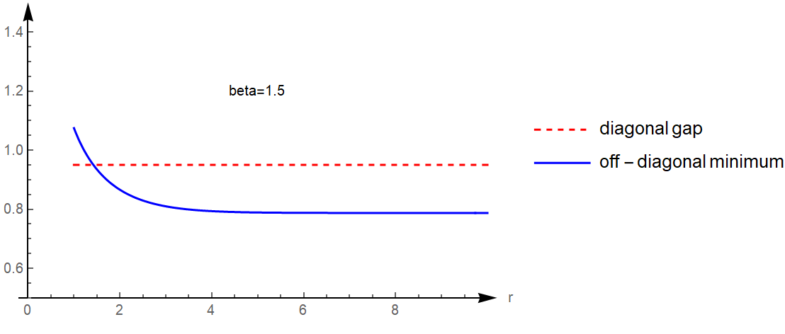
Figure 1: Diagonal lower bound and off-diagonal minimum, $\beta=1.5$, $q=1$.

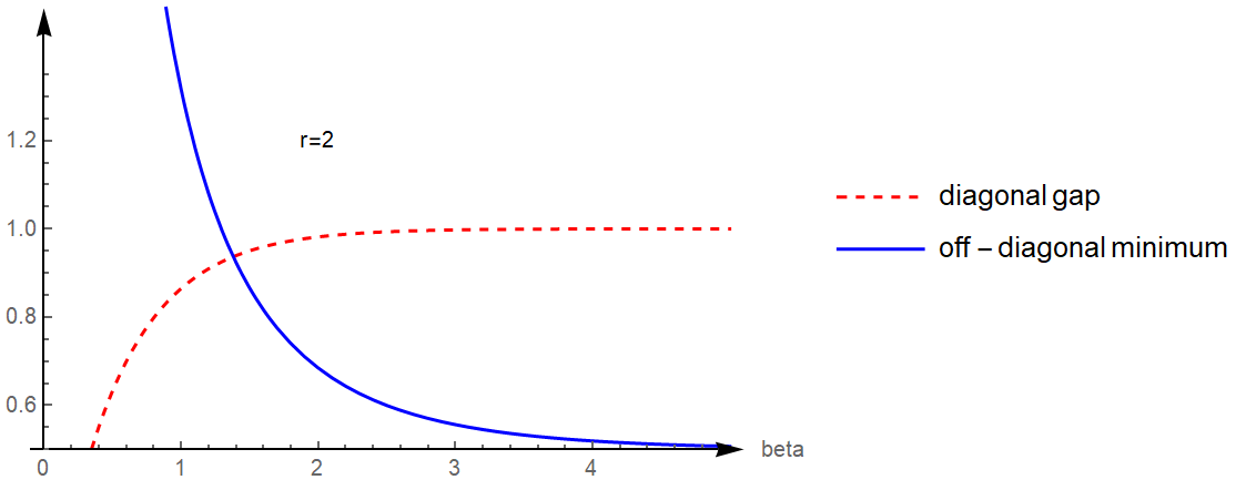
Figure 2: Diagonal lower bound and off-diagonal minimum, $r=2$.

In order to better understand which one among the off-diagonal minimum and the diagonal spectral gap is bigger and convince ourselves that, for $\beta$ small, the spectral gap of the generator $L$ is actually given by the spectral gap of $\mathcal{A}$, not just because of a poor estimate of the lower bound of Theorem 5.5, we can study the upper bound of the diagonal spectral gap.

In Appendix B, by choosing a special $f$ and evaluating $-\langle f,\mathcal{A}f\rangle/\|f\|^{2}$, we found

$$\operatorname{gap}(\mathcal{A})\leq 1/\big{(}\big{(}{\rm e}^{\beta}-1\big{)}\big{(}1-Z_{\beta}^{-1}\big{)}\big{)}$$

showing that if $\beta$ is sufficiently small and $r>1$, $q<1$ are sufficiently near to $1$, then the spectral gap of the generator $L$ coincides with the one of $\mathcal{A}$ the diagonal subalgebra. Moreover, we showed that the lower bound of Theorem 5.5 is near the optimal one for big $\beta$.

Summing up, from Proposition 5.1, Theorems 5.3 and 5.5, we get the following

Theorem 5.6.

Suppose that $-1\leq q\leq 1<r$ with $r+q-2\geq 0$. Then for all $\beta>0$,

$$\operatorname{gap}(L)=\min\left\{1-{\rm e}^{-2\beta},\,\frac{1}{2}\left(\frac{{\rm e}^{\beta}+1}{{\rm e}^{\beta}-1}+\frac{r+q}{{\rm e}^{\beta(r+q-1)}-1}\right)\right\}.$$

Appendix A Inequalities for partial sums

We collect here estimates on partial sums of series needed in the evaluation of the spectral gap.

Lemma A.1.

For all $u\in\mathbb{N}$ we have

$$\frac{\sum_{y>u}(y-u)\pi_{y}}{\pi_{u}\lambda_{u}}\leq\frac{1}{\varepsilon_{u+1}\big{(}1-{\rm e}^{-\beta\omega_{u+1}}\big{)}}.$$

Proof.

Recalling that the sequence $(\omega_{k})_{k\geq 1}$ is non-decreasing, by $r+q-2\geq 0$, we can write

$$\frac{\sum_{y>u}(y-u)\pi_{y}}{\pi_{u}\lambda_{u}} =\frac{{\rm e}^{\beta\omega_{u+1}}-1}{\varepsilon_{u+1}}\sum_{y>u}(y-u){\rm e}^{-\beta(\varepsilon_{y}-\varepsilon_{u})}=\frac{{\rm e}^{\beta\omega_{u+1}}-1}{\varepsilon_{u+1}}\sum_{y>u}(y-u){\rm e}^{-\beta\sum_{j=u+1}^{y}\omega_{j}}$$

$$\leq\frac{{\rm e}^{\beta\omega_{u+1}}-1}{\varepsilon_{u+1}}\sum_{y>u}(y-u){\rm e}^{-\beta(y-u)\omega_{u+1}}=\frac{1}{\varepsilon_{u+1}\left(1-{\rm e}^{-\beta\omega_{u+1}}\right)}.$$ ∎

Lemma A.2.

For all $u\in\mathbb{N}$, $u\geq 1$, we have

$$\sum_{x=0}^{u-1}(u-x)\pi_{x}\leq\frac{u}{1-{\rm e}^{-\beta}}-\frac{{\rm e}^{-\beta}\big{(}1-{\rm e}^{-\beta u}\big{)}}{\big{(}1-{\rm e}^{-\beta}\big{)}^{2}},$$

$$\sum_{x=0}^{u}\pi_{x}\leq\frac{1-{\rm e}^{-\beta(u+1)}}{1-{\rm e}^{-\beta}}.$$

Proof.

Notice that $\varepsilon_{x}=\sum_{j=1}^{x}\omega_{j}\geq x\omega_{1}=x$ (inequality (5.6)). Then both follow from the explicit summation formulae. ∎

Lemma A.3.

For the tail of the invariant measure we have the bound.

$$\pi_{u+1}\leq\sum_{y>u}\pi_{y}\leq\frac{\pi_{u+1}}{1-{\rm e}^{-\beta\omega_{u+1}}}.$$

Proof.

The lower bound is obvious. For the upper bound,

$$\sum_{y>u}\pi_{y} =\sum_{y>u}{\rm e}^{-\beta\varepsilon_{y}}={\rm e}^{-\beta\varepsilon_{u}}\sum_{y>u}{\rm e}^{-\beta(\varepsilon_{y}-\varepsilon_{u})}={\rm e}^{-\beta\varepsilon_{u}}\sum_{y>u}{\rm e}^{-\beta\sum_{j=u+1}^{y}\omega_{j}}$$

$$\leq{\rm e}^{-\beta\varepsilon_{u}}\sum_{y>u}{\rm e}^{-\beta(y-u)\omega_{u+1}}={\rm e}^{-\beta\varepsilon_{u}}\frac{{\rm e}^{-\beta\omega_{u+1}}}{1-{\rm e}^{-\beta\omega_{u+1}}}=\frac{{\rm e}^{-\beta\varepsilon_{u+1}}}{1-{\rm e}^{-\beta\omega_{u+1}}}=\frac{\pi_{u+1}}{1-{\rm e}^{-\beta\omega_{u+1}}}.$$ ∎

Appendix B An upper bound for the diagonal spectral gap

We first consider the limiting case: $r\to 1^{+}$, $q\to 1^{-}$. In that case the jump rates become

$$\lambda_{n}(\beta,r,q)\underset{r\to 1^{+},\,q\to 1^{-}}{\longrightarrow}\lambda_{n}(\beta,1,1)=\frac{n+1}{{\rm e}^{\beta}-1},\qquad\mu_{n}(\beta,r,q)\underset{r\to 1^{+},\,q\to 1^{-}}{\longrightarrow}\mu_{n}(\beta,1,1)=\frac{n\,{\rm e}^{\beta}}{{\rm e}^{\beta}-1}$$

and, for small $\beta$ (i.e., high temperatures), the diagonal spectral gap is near $1$ as expected by [10, Section 5] or [13, Section 7].

Next, we find an upper bound with a simple $(f_{n})_{n\geq 0}$. Define for $u\geq 0$, $Z_{\beta}(u):=\sum_{x\geq u}\pi_{x}$; $Z_{\beta}:=Z_{\beta}(0)$. Put $f=(f_{n})_{n\geq 0}$ as

$$f_{0}=1,\qquad f_{n}=-c,\quad\text{for }n\geq 1,$$

where $c$ is chosen so that $\sum_{x\geq 0}f_{x}\pi_{x}=0$, and hence $c=\pi_{0}/Z_{\beta}(1)=1/(Z_{\beta}-1)$,

$$\mathcal{E}(f)=\sum_{x=0}^{\infty}\tilde{\pi}_{x}\lambda_{x}(f_{x+1}-f_{x})^{2}=Z_{\beta}^{-1}\pi_{0}\lambda_{0}(1+c)^{2}=\frac{Z_{\beta}\,\lambda_{0}}{Z_{\beta}(1)^{2}},$$

$$\|f\|^{2}=\sum_{x=0}^{\infty}\tilde{\pi}_{x}f_{x}^{2}=Z_{\beta}^{-1}\left(\pi_{0}+c^{2}Z_{\beta}(1)\right)=\frac{1}{Z_{\beta}(1)}.$$

Therefore,

$${\rm gap}(\mathcal{A})\leq\frac{Z_{\beta}\,\lambda_{0}}{Z_{\beta}(1)}=\frac{1}{\big{(}{\rm e}^{\beta}-1\big{)}\big{(}1-Z_{\beta}^{-1}\big{)}}:=\alpha(\beta,r,q).$$

Noticing that $\alpha(\beta,r,q)$ is continuous with respect to both $\beta>0$, $r>1$ and $0<q<1$

$$\alpha(\beta,1,1):=\lim_{r\to 1^{+},\,q\to 1^{-}}\alpha(\beta,r,q)=\frac{1}{1-{\rm e}^{-\beta}}.$$

On the other hand, comparing with the off-diagonal minimum for $r=q=1$, which is $\big{(}1+3{\rm e}^{-\beta}\big{)}/2\big{(}1-{\rm e}^{-\beta}\big{)}$, we see that when $0<\beta<\log 3$,

$$\frac{1}{1-{\rm e}^{-\beta}}<\frac{1+3{\rm e}^{-\beta}}{2\big{(}1-{\rm e}^{-\beta}\big{)}},$$

which says, together with the continuity of both $\alpha(\beta,r,q)$ and the formula of off-diagonal minimum, that if $\beta$ is sufficiently small and $r>1$, $q<1$ are sufficiently near to $1$, then the spectral gap of the QMS occurs at the diagonal subalgebra.

Fix $q=1$ and let’s find regions in the $r$-$\beta$ plane to see which gap would dominates. In Figure 3, the upper line is the level curve found by equating the off-diagonal minimum and the diagonal lower bound, $1-{\rm e}^{-2\beta}$. In the above the curve, the off-diagonal minimum is less than the lower bound of the diagonal gap, and hence in that region the spectral gap occurs in the off-diagonal subspace. Similarly, the lower line in the figure is the level curve obtained by equating the off-diagonal minimum and the upper bound of the diagonal gap, $\alpha(\beta,r,1)$. In the region below the curve, the off-diagonal minimum dominates the diagonal upper bound and therefore the spectral gap occurs in the diagonal subspace.

Figure 3: Gap dominators: above the upper curve, the spectral gap occurs at off-diagonal subspaces and below the lower curve, the spectral gap occurs at the diagonal subspace ($q=1$, horizontal axis for $r$ and vertical axis for $\beta$).

Acknowledgements

The work of HJY was supported by the National Research Foundation of Korea (NRF) grant funded by the Korean government (MSIT) (no. 2020R1F1A101075). FF is a member of GNAMPA-INdAM Italy. FF first met Michael Schürmann at the conference Quantum Probability and Applications III held in Oberwolfach, January 25–31, 1987, organized by their respective advisors Professors Luigi Accardi and Wilhelm von Waldenfels [30]. Over most of these years he has had the pleasure of meeting him at the annual QP conferences, that nowadays reached the number 42, visiting him in Greifswald, exchange views and follow reports on his scientific work. He would like to congratulate Michael on his retirement and wish him endless happy days with his friends and family.

References

• [1] Accardi L., García-Corte J.C., Guerrero-Poblete F., Quezada R., Breaking of the similarity principle in Markov generators of low density limit type and the role of degeneracies in the landscape of invariant states, Open Syst. Inf. Dyn. 27 (2020), 2050018, 40 pages.
• [2] Accardi L., Lu Y.G., The Wigner semi-circle law in quantum electrodynamics, Comm. Math. Phys. 180 (1996), 605–632.
• [3] Accardi L., Lu Y.G., Volovich I., Quantum theory and its stochastic limit, Springer-Verlag, Berlin, 2002.
• [4] Anderson W.J., Continuous-time Markov chains: an applications-oriented approach, Springer Series in Statistics: Probability and its Applications, Springer-Verlag, New York, 1991.
• [5] Becker S., Datta N., Salzmann R., Quantum Zeno effect in open quantum systems, Ann. Henri Poincaré 22 (2021), 3795–3840, arXiv:2010.04121.
• [6] Blitvić N., The $(q,t)$-Gaussian process, J. Funct. Anal. 263 (2012), 3270–3305.
• [7] Bożejko M., Remarks on $q$-CCR relations for $|q|>1$, in Noncommutative Harmonic Analysis with Applications to Probability, Banach Center Publ., Vol. 78, Polish Acad. Sci. Inst. Math., Warsaw, 2007, 59–67.
• [8] Bożejko M., Kümmerer B., Speicher R., $q$-Gaussian processes: non-commutative and classical aspects, Comm. Math. Phys. 185 (1997), 129–154, arXiv:funct-an/9604010.
• [9] Bożejko M., Lytvynov E., Wysoczański J., Fock representations of $Q$-deformed commutation relations, J. Math. Phys. 58 (2017), 073501, 19 pages, arXiv:1603.03075.
• [10] Carbone R., Fagnola F., Exponential $L_{2}$-convergence of quantum Markov semigroups on $\mathcal{B}(h)$, Math. Notes 68 (2000), 452–463.
• [11] Carbone R., Sasso E., Umanità V., Structure of generic quantum Markov semigroup, Infin. Dimens. Anal. Quantum Probab. Relat. Top. 20 (2017), 1750012, 19 pages.
• [12] Carlen E.A., Maas J., Gradient flow and entropy inequalities for quantum Markov semigroups with detailed balance, J. Funct. Anal. 273 (2017), 1810–1869, arXiv:1609.01254.
• [13] Cipriani F., Fagnola F., Lindsay J.M., Spectral analysis and Feller property for quantum Ornstein–Uhlenbeck semigroups, Comm. Math. Phys. 210 (2000), 85–105.
• [14] Daoud M., Kibler M., Statistical mechanics of $qp$-bosons in $D$ dimensions, Phys. Lett. A 206 (1995), 13–17, arXiv:quant-ph/9512006.
• [15] Deschamps J., Fagnola F., Sasso E., Umanità V., Structure of uniformly continuous quantum Markov semigroups, Rev. Math. Phys. 28 (2016), 1650003, 32 pages, arXiv:1412.3239.
• [16] Dhahri A., Fagnola F., Yoo H.J., Quadratic open quantum harmonic oscillator, Lett. Math. Phys. 110 (2020), 1759–1782, arXiv:1905.09965.
• [17] Fagnola F., Quantum Markov semigroups and quantum flows, Proyecciones 18 (1999), 95–134.
• [18] Fagnola F., Quezada R., A characterization of quantum Markov semigroups of weak coupling limit type, Infin. Dimens. Anal. Quantum Probab. Relat. Top. 22 (2019), 1950008, 10 pages.
• [19] Fagnola F., Umanità V., Generic quantum Markov semigroups, cycle decomposition and deviation from equilibrium, Infin. Dimens. Anal. Quantum Probab. Relat. Top. 15 (2012), 1250016, 17 pages.
• [20] Gavrilik A.M., Kachurik I.I., Nonstandard deformed oscillators from $q$- and $p,q$-deformations of Heisenberg algebra, SIGMA 12 (2016), 047, 12 pages, arXiv:1602.07927.
• [21] Gerhold M., Skeide M., Interacting Fock spaces and subproduct systems, Infin. Dimens. Anal. Quantum Probab. Relat. Top. 23 (2020), 2050017, 53 pages, arXiv:1808.07037.
• [22] Gough J., Kupsch J., Quantum fields and processes: a combinatorial approach, Cambridge Studies in Advanced Mathematics, Vol. 171, Cambridge University Press, Cambridge, 2018.
• [23] Kumar D., Sinha K.B., Srivastava S., Stability of the Markov (conservativity) property under perturbations, Infin. Dimens. Anal. Quantum Probab. Relat. Top. 23 (2020), 2050009, 20 pages.
• [24] Liggett T.M., Exponential $L_{2}$ convergence of attractive reversible nearest particle systems, Ann. Probab. 17 (1989), 403–432.
• [25] Marinho A.A., Brito F.A., Hermite polynomials and Fibonacci oscillators, J. Math. Phys. 60 (2019), 012101, 9 pages, arXiv:1805.03229.
• [26] Mouayn Z., El Moize O., A generalized Euler probability distribution, Rep. Math. Phys. 87 (2021), 291–311.
• [27] Mukhamedov F., Al-Rawashdeh A., Generalized Dobrushin ergodicity coefficient and uniform ergodicities of Markov operators, Positivity 24 (2020), 855–890, arXiv:2001.06266.
• [28] Mukhamedov F., Al-Rawashdeh A., Generalized Dobrushin ergodicity coefficient and ergodicities of non-homogeneous Markov chains, Banach J. Math. Anal. 16 (2022), 18, 37 pages, arXiv:2001.07703.
• [29] Parthasarathy K.R., An introduction to quantum stochastic calculus, Modern Birkhäuser Classics, Birkhäuser/Springer Basel AG, Basel, 1992.
• [30] Schürmann M., von Waldenfels W., A central limit theorem on the free Lie group, in Quantum Probability and Applications, III (Oberwolfach, 1987), Lecture Notes in Math., Vol. 1303, Springer, Berlin, 1988, 300–318.
\LastPageEnding