Abstract

In modern classification tasks, the number of labels is getting larger and larger, as is the size of the datasets encountered in practice. As the number of classes increases, class ambiguity and class imbalance become more and more problematic to achieve high top-$1$ accuracy. Meanwhile, Top-$K$ metrics (metrics allowing $K$ guesses) have become popular, especially for performance reporting. Yet, proposing top-$K$ losses tailored for deep learning remains a challenge, both theoretically and practically. In this paper we introduce a stochastic top-$K$ hinge loss inspired by recent developments on top-$K$ calibrated losses. Our proposal is based on the smoothing of the top-$K$ operator building on the flexible ”perturbed optimizer” framework. We show that our loss function performs very well in the case of balanced datasets, while benefiting from a significantly lower computational time than the state-of-the-art top-$K$ loss function. In addition, we propose a simple variant of our loss for the imbalanced case. Experiments on a heavy-tailed dataset show that our loss function significantly outperforms other baseline loss functions.

1 Introduction

Fine-grained visual categorization (FGVC) has recently attracted a lot of attention Wang et al. (2022), in particular in the biodiversity domain Horn et al. (2018); Garcin et al. (2021); Van Horn et al. (2015). In FGVC, one aims to classify an image into subordinate categories (such as plant or bird species) that contain many visually similar instances. The intrinsic ambiguity among the labels makes it difficult to obtain high levels of top-1 accuracy as is typically the case with standard datasets such as CIFAR10 Krizhevsky (2009) or MNIST LeCun et al. (1998). For systems like Merlin Van Horn et al. (2015) or Pl@ntNet Affouard et al. (2017), due to the difficulty of the task, it is generally relevant to provide the user with a set of classes in the hope that the true class belongs to that set. In practical applications, the display limit of the device only allows to give a few labels back to the user. A straightforward strategy consists in returning a set of $K$ classes for each input, where $K$ is a small integer with respect to the total number of classes. Such classifiers are called top-$K$ classifiers, and their performance is evaluated with the well known top-$K$ accuracy Lapin et al. (2015); Russakovsky et al. (2015). While such a metric is very popular for evaluating applications, common learning strategies typically consist in learning a deep neural network with the cross-entropy loss, neglecting the top-$K$ constraint in the learning step.

Yet, recent works have focused on optimizing the top-$K$ accuracy directly. Lapin et al. (2015) have introduced the top-$K$ hinge loss and a convex upper-bound, following techniques introduced by Usunier et al. (2009) for ranking. A limit of this approach was raised by Berrada et al. (2018), as they have shown that the top-$K$ hinge loss by Lapin et al. (2015) can not be directly used for training a deep neural network. The main arguments put forward by the authors to explain this practical limitation are: (i) the non-smoothness of the top-$K$ hinge loss and (ii), the sparsity of its gradient. Consequently, they propose a smoothed alternative adjustable with a temperature parameter. However, their smoothing procedure is computationally costly when $K$ increases (as demonstrated in our experiments), despite the efficient algorithm they provide to cope with the combinatorial nature of the loss. Moreover, this approach has the drawback to be specific to the top-$K$ hinge loss introduced by Lapin et al. (2015).

In contrast, we propose a new top-$K$ loss that relies on the smoothing of the top-$K$ operator (the operator returning the $K$-th largest value of a vector). The smoothing framework we consider, the perturbed optimizers (Berthet et al., 2020), can be used to smooth variants of the top-$K$ hinge loss but could independently be considered for other learning tasks such as $K$-nearest neighbors or top-$K$ recommendation (He et al., 2019; Covington et al., 2016). Additionally, we introduce a simple variant of our loss to deal with imbalanced datasets. Indeed, for many real-world applications, a long-tailed phenomenon appears Reed (2001): a few labels enjoy a lot of items (e.g., images), while the vast majority of the labels receive only a few items, see for instance a dataset like Pl@ntnet-300k (Garcin et al., 2021) for a more quantitative overview. We find that the loss by Berrada et al. (2018) fails to provide satisfactory results on the tail classes in our experiments. On the contrary, our proposed loss based on uneven margins outperforms the loss from Berrada et al. (2018) and the LDAM loss (Cao et al., 2019), a loss designed for imbalance cases known for its very good performance in fine-grained visual classification challenges (Wang et al., 2021). To the best of our knowledge, our proposed loss is the first loss function tackling both the top-$K$ classification and class imbalance problems jointly.

2 Related work

Several top-$K$ losses have been introduced and experimented with in Lapin et al. (2015; 2016; 2017). However, the authors assume that the inputs are features extracted from a deep neural network and optimize their losses with SDCA Shalev-Shwartz & Zhang (2013). Berrada et al. (2018) have shown that the top-$K$ hinge loss from Lapin et al. (2015) could not be directly used in a deep learning optimization pipeline. Instead, we are interested in end-to-end deep neural network learning. The state-of-the art top-$K$ loss for deep learning is that of Berrada et al. (2018), which is a smoothing of a top-$K$ hinge loss by Lapin et al. (2015). The principle of the top-$K$ loss of Berrada et al. (2018) is based on the rewriting the top-$K$ hinge loss of Lapin et al. (2015) as a difference of two maxes on a combinatorial number of terms, smooth the max with the logsumexp, and use a divide-and-conquer approach to make their loss tractable. Instead, our approach relies on smoothing the top-$K$ operator and using this smoothed top-$K$ operator on a top-$K$ calibrated loss recently proposed by Yang & Koyejo (2020). Our approach could be used out-of-the box with other top-$K$ hinge losses. In contrast, the smoothing method of Berrada et al. (2018) is tailored for the top-$K$ hinge loss of Lapin et al. (2015), which is shown to be not top-$K$ calibrated in Yang & Koyejo (2020).

For a general theory of smoothing in optimization, we refer the reader to Beck & Teboulle (2012); Nesterov (2005) while for details on perturbed optimizers, we refer the reader to Berthet et al. (2020) and references therein. In the literature, other alternatives have been proposed to perform top-$K$ smoothing. Xie et al. (2020) formulate the smooth top-$K$ operator as the solution of a regularized optimal transport problem between well-chosen discrete measures. The authors rely on a costly optimization procedure to compute the optimal plan. Xie & Ermon (2019) propose a smoothing of the top-$K$ operator through $K$ successive softmax. Besides the additional cost with large $K$, the computation of $K$ successive softmax brings numerical instabilities.

Concerning imbalanced datasets, several recent contributions have focused on architecture design (Zhou et al., 2020; Wang et al., 2021). Instead, we focus here on the design of the loss function and leverage existing popular neural networks architectures. A popular loss for imbalanced classification is the focal loss (Lin et al., 2017) which is a modification of the cross entropy where well classified-examples induce a smaller loss, putting emphasis on difficult examples. Instead, we use uneven margins in our formulation, requiring examples of the rarest classes to be well classified by a larger margin than examples of the most common classes. Uneven margin losses have been studied in the binary case in (Scott, 2012; Li & Shawe-Taylor, 2003; Iranmehr et al., 2019). For the multi-class setting, the LDAM loss (Cao et al., 2019) is a widely used uneven margin loss which can be seen as a cross entropy incorporating uneven margins in the logits. Instead, our imbalanced top-$K$ loss relies on the smoothing of the top-$K$ operator.

3 Proposed method

(a) Top-$K$: C
$\ell=\ell^{K}$.$\ell=\ell_{\textrm{Cal.~{}Hinge}}^{K}$

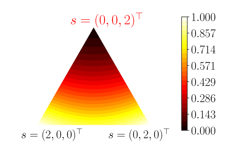
(b) Cross-entropy:
$\ell=\ell_{\textrm{CE}}$.$\ell=\ell_{\textrm{Cal.~{}Hinge}}^{K}$

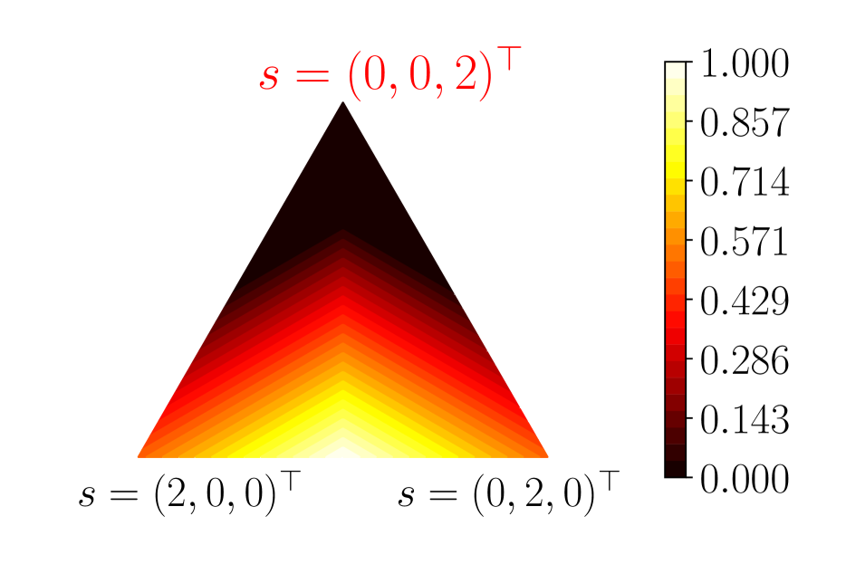
(c) Multi-class hinge:
$\ell=\ell_{\textrm{Hinge}}^{K}$.

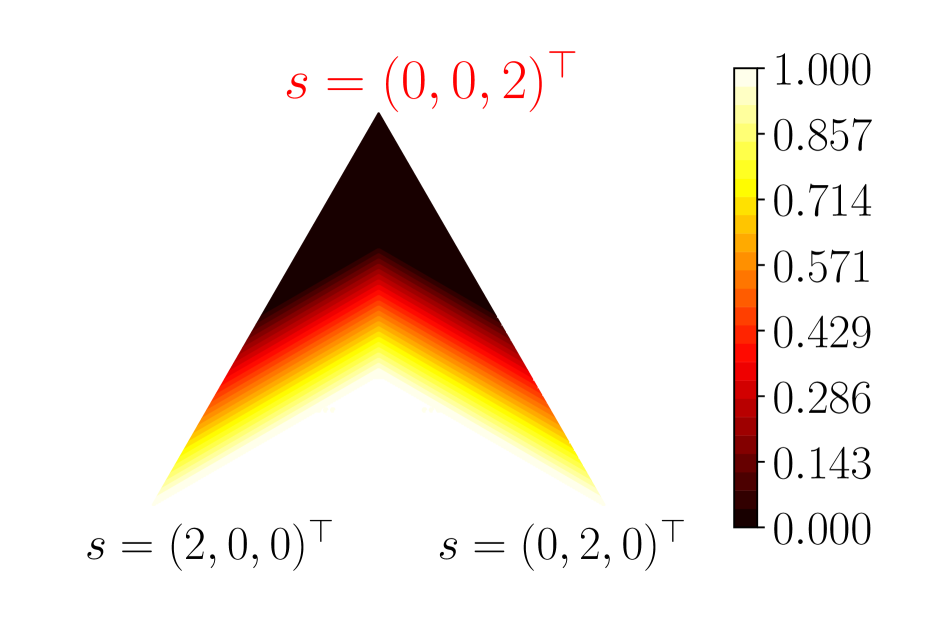
(d) Calibrated hinge:
$\ell=\ell_{\textrm{Cal.~{}Hinge}}^{K}$.

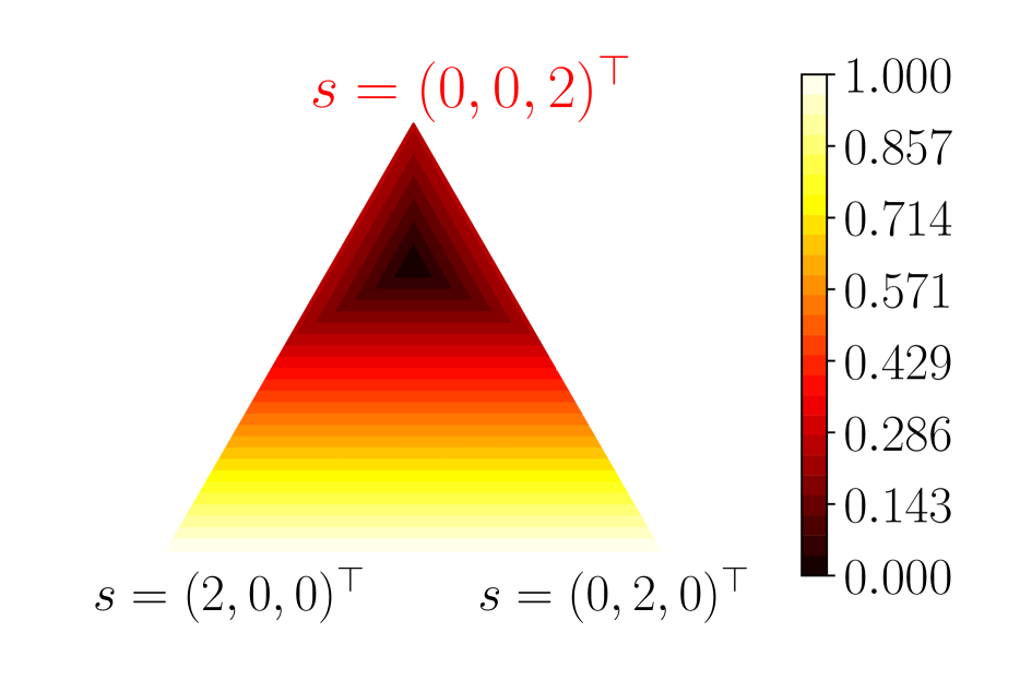
(e) Convexified hinge:
$\ell=\ell_{\textrm{CVXHinge}}^{K}$.

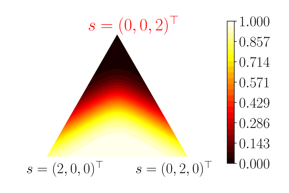
(f) Smoothed hinge
$\ell_{\text{Smoothed Hinge}}^{K,0.1}$.

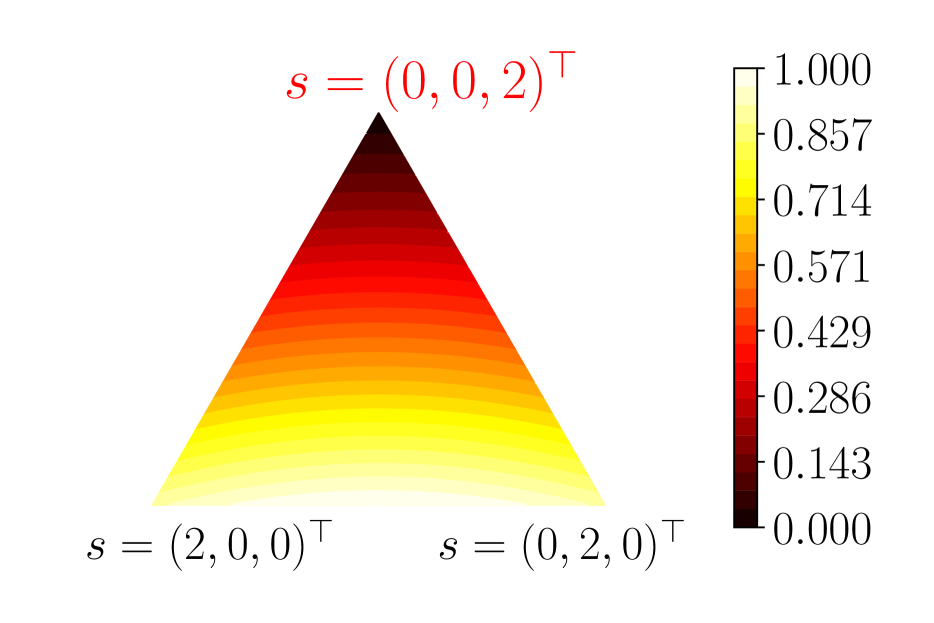
(g) Smoothed hinge
$\ell_{\text{Smoothed Hinge}}^{K,1}$.

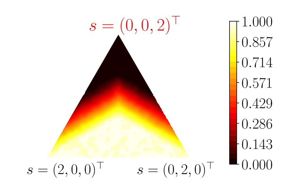
(h) Noised balanced: g
$\ell_{\text{Noised bal.}}^{K,0.3,30}$. $\ell_{\text{Smoothed Hinge}}^{K,0.4}$

(i) Noised balanced: g
$\ell_{\text{Noised bal.}}^{K,1,30}$. $\ell_{\text{Smoothed Hinge}}^{K,0.4}$

(j) Noised imbalanced: g
$\ell_{\text{Noised Imbal.}}^{K,1,30,5}$. $\ell_{\text{Smoothed Hinge}}^{K,0.4}$

Figure 1: Level sets of the function $\mathbf{s}\mapsto\ell(\mathbf{s},y)$ for different losses described in Table 1, for $L=3$ classes, $K=2$ and a true label $y=3$ (corresponding to the upper corner of the triangles). For visualization the loss are rescaled between 0 and 1, and the level sets are restricted to vector $\mathbf{s}\in 2\cdot\Delta_{3}$. The losses have been harmonized to display a margin equal to 1. For our proposed loss, we have averaged the level sets over 100 replications to avoid meshing artifacts.

Table 1: Summary of standard top-$K$ losses: vanilla top-$K$ $\ell^{K}$; Cross Entropy $\ell_{\textrm{CE}}$; hinge top-$K$ $\ell_{\textrm{Hinge}}^{K}$; Convexified hinge top-$K$ $\ell_{\textrm{CVXHinge}}^{K}$; Calibrated hinge top-$K$ $\ell_{\textrm{Cal.~{}Hinge}}^{K}$; Log-sum Smoothed hinge top-$K$ $\ell_{\text{Smoothed Hinge}}^{K,\tau}$; Noised balanced hinge top-$K$ $\ell_{\text{Noised bal.}}^{K,\epsilon,B}$ (proposed); Noised imbalanced hinge top-$K$ $\ell_{\text{Noised Imbal.}}^{K,\epsilon,B,m_{y}}$ (proposed).

Loss : $\ell(\mathbf{s},y)$	Expression	Param.	Reference
$\ell^{K}(\mathbf{s},y)$	$\mathds{1}_{\{\mathrm{top}_{K}(\mathbf{s})>s_{y}\}}$	$K$	Equation 3
$\ell_{\textrm{CE}}(\mathbf{s},y)$	$-\ln\Big{(}e^{s_{y}}/\sum_{k\in[L]}e^{s_{k}}\Big{)}$	—
$\ell_{\textrm{LDAM}}^{m_{y}}(\mathbf{s},y)$	$-\ln\Big{(}e^{s_{y}-m_{y}}/\big{[}e^{s_{y}-m_{y}}+\sum_{k\in[L],k\neq y}e^{s_{k}}\big{]}\Big{)}$	$m_{y}$	(Lin et al., 2017)
$\ell_{\textrm{focal}}^{\gamma}(\mathbf{s},y)$	$(1-\log\left[\ell_{\textrm{CE}}(\mathbf{s},y)\right]\Big{)}^{\gamma}\ell_{\textrm{CE}}(\mathbf{s},y)$	$\gamma$	(Cao et al., 2019)
$\ell_{\textrm{Hinge}}^{K}(\mathbf{s},y)$	$\left(1+\mathrm{top}_{K}(\mathbf{s}_{\setminus y})-s_{y}\right)_{+}$	$K$	Equation 4, Lapin et al. (2015)
$\ell_{\textrm{CVXHinge}}^{K}(\mathbf{s},y)$	$\left(\frac{1}{K}\sum_{k\in[K]}\mathrm{top}_{k}(\mathbf{1}_{L}-\delta_{y}+\mathbf{s})-s_{y}\right)_{+}$	$K$	Lapin et al. (2015)
$\ell_{\textrm{Cal.~{}Hinge}}^{K}(\mathbf{s},y)$	$(1+\mathrm{top}_{K+1}(\mathbf{s})-s_{y})_{+}$	$K$	Equation 17, Yang & Koyejo (2020)
$\ell_{\text{Smoothed Hinge}}^{K,\tau}(\mathbf{s},y)$	$\begin{aligned} \displaystyle\tau\ln\Big{[}\sum_{\begin{subarray}{c}A\subset[L],|A|=K\end{subarray}}e^{\tfrac{\mathds{1}_{\{y\notin A\}}}{\tau}+\sum\limits_{j\in A}\tfrac{s_{j}}{K\tau}}\Big{]}-\tau\ln\Big{[}\sum_{\begin{subarray}{c}A\subset[L],|A|=K\end{subarray}}e^{\sum\limits_{j\in A}\tfrac{s_{j}}{K\tau}}\Big{]}\end{aligned}$	$K$, $\tau$	Berrada et al. (2018)
$\ell_{\text{Noised bal.}}^{K,\epsilon,B}(\mathbf{s},y)$	$(1+\widehat{\mathrm{top}}_{K+1,\epsilon,B}(\mathbf{s})-s_{y})_{+}$, where $\widehat{\mathrm{top}}_{K+1,\epsilon,B}(\mathbf{s})$ is the noisy top-$K+1$	$K$, $\epsilon$, $B$	Equation 8, (proposed)
$\ell_{\text{Noised Imbal.}}^{K,\epsilon,B,m_{y}}(\mathbf{s},y)$	$(m_{y}+\widehat{\mathrm{top}}_{K+1,\epsilon,B}(\mathbf{s})-s_{y})_{+}$, where $\widehat{\mathrm{top}}_{K+1,\epsilon,B}(\mathbf{s})$ is the noisy top-$K+1$	$K$, $\epsilon$, $B$, $m_{y}$	Equation 13, (proposed)

3.1 Preliminaries

Following classical notation, we deal with multi-class classification that considers the problem of learning a classifier from $\mathcal{X}$ to $[L]\triangleq\{1,\dots,L\}$ based on $n$ pairs of (input, label) i.i.d. sampled from a joint distribution $\mathbb{P}$: $(x_{1},y_{1}),\dots,(x_{n},y_{n})\in\mathcal{X}\times[L]$, where $\mathcal{X}$ is the input data space ($\mathcal{X}$ is the space of RGB images of a given size in our vision applications) and the $y$’s are the associated labels among $L$ possible ones.

For a training pair of observed features and label $(x,y)$, $\mathbf{s}\in\mathbb{R}^{L}$ refers to the associated score vector (often referred to as logits). From now on, we use bold font to represent vectors. For $k\in[L]$, $s_{k}$ refers to the score attributed to the $k$-th class while $s_{y}$ refers to the score of the true label and $s_{(k)}$ refers to the $k$-th largest score, so that $s_{(1)}\geq\dots\geq s_{(k)}\geq\dots\geq s_{(L)}$. For $K\in[L]$, we define $\mathrm{top}_{K}$ and $\mathrm{top}\Sigma_{K}$, functions from $\mathbb{R}^{L}$ to $\mathbb{R}$ as:

$$\mathrm{top}_{K} :\mathbf{s}\mapsto s_{(K)}$$ (1)

$$\mathrm{top}\Sigma_{K} :\mathbf{s}\mapsto\sum_{k\in[K]}s_{(k)}\enspace.$$ (2)

We write $\mathbf{1}_{L}=(1,\dots,1)^{\top}\in\mathbb{R}^{L}$. For $\mathbf{s}\in\mathbb{R}^{L}$, the gradient $\nabla\mathrm{top}_{K}(\mathbf{s})$ is a vector with a single one at the $K$-th largest coordinate of $\mathbf{s}$ and 0 elsewhere (denoted as $\mathrm{arg\,top}_{K}(\mathbf{s})$). Similarly, $\nabla\mathrm{top}\Sigma_{K}(\mathbf{s})$ is a vector with $K$ ones at the $K$ largest coordinates of $\mathbf{s}$ and 0 elsewhere (denoted as $\mathrm{arg\,top}\Sigma_{K}(\mathbf{s})$).

The top-$K$ loss (a 0/1 loss) can now be written

$$\ell^{K}(\mathbf{s},y)=\mathds{1}_{\{\mathrm{top}_{K}(\mathbf{s})>s_{y}\}}\enspace.$$ (3)

This loss reports an error when the score of the true label $y$ is not among the $K$-th largest scores. One would typically seek to minimize this loss. Yet, being a piece-wise constant function w.r.t. to its first argument, numerical difficulties make solving this problem particularly hard in practice. In what follows we recall some popular surrogate top-$K$ losses from the literature before providing new alternatives. We summarize such variants in Table 1 and illustrate their differences in Figure 1 for $L=3,K=2$ (see also Figure 6 in Appendix, for $L=3,K=1$).

A first alternative introduced by Lapin et al. (2015) is a relaxation generalizing the multi-class hinge loss introduced by Crammer & Singer (2001) to the top-$K$ case:

$$\ell_{\textrm{Hinge}}^{K}(\mathbf{s},y)=\left(1+\mathrm{top}_{K}(\mathbf{s}_{\setminus y})-s_{y}\right)_{+}\enspace,$$ (4)

where $\mathbf{s}_{\setminus y}$ is the vector in $\mathbb{R}^{d-1}$ obtained by removing the $y$-th coordinate of $\mathbf{s}$, and $(\cdot)_{+}\triangleq\max(0,\cdot)$. The authors propose a convex loss function $\ell_{\textrm{CVXHinge}}^{K}$ (see Table 1) which upper bounds the loss function $\ell_{\textrm{Hinge}}^{K}$.

Berrada et al. (2018) have proposed a smoothed counterpart of $\ell_{\textrm{Hinge}}^{K}$, relying on a recursive algorithm tailored for their combinatorics smoothed formulation. Yet, a theoretical limitation of $\ell_{\textrm{Hinge}}^{K}$ and $\ell_{\textrm{CVXHinge}}^{K}$ was raised by Yang & Koyejo (2020) showing that they are not top-$K$ calibrated. Top-$K$ calibration is a property defined by Yang & Koyejo (2020). We recall some technical details in Appendix A and the precise definition of top-$K$ calibration is given in Definition A.2.

We let $\Delta_{L}\triangleq\{\boldsymbol{\pi}\in\mathbb{R}^{L}:\sum_{k\in[L]}\pi_{k}=1,\pi_{k}\geq 0\}$ denote the probability simplex of size $L$. For a score $\mathbf{s}\in\mathbb{R}^{L}$ and $\boldsymbol{\pi}\in\Delta_{L}$ representing the conditional distribution of $y$ given $x$, we write the conditional risk at $x\in\mathcal{X}$ as $\mathcal{R}_{\ell|x}(\mathbf{s},\boldsymbol{\pi})=\mathbb{E}_{y|x\sim\pi}(\ell(\mathbf{s},y))$ and the (integrated) risk as $\mathcal{R}_{\ell}(f)\triangleq\mathbb{E}_{(x,y)\sim\mathbb{P}}[\ell(f(x),y)]$ for a scoring function $f:\mathcal{X}\to\mathbb{R}^{L}$. The associated Bayes risks are defined respectively by $\mathcal{R}_{\ell|x}^{*}(\boldsymbol{\pi})\triangleq\inf_{\mathbf{s}\in\mathbb{R}^{L}}\mathcal{R}_{\ell|x}(\mathbf{s},\boldsymbol{\pi})$ and $\mathcal{R}_{\ell}^{*}\triangleq\inf_{f:\mathcal{X}\to\mathbb{R}^{L}}\mathcal{R}_{\ell}(f)$. The following result by (Yang & Koyejo, 2020) shows that a top-$K$ calibrated loss is top-$K$ consistent, meaning that a minimizer of such a loss would also lead to Bayes optimal classifiers:

Theorem 3.1.

(Yang & Koyejo, 2020, Theorem 2.2). Suppose $\ell$ is a nonnegative top-$K$ calibrated loss function. Then, $\ell$ is top-$K$ consistent, i.e., for any sequence of measurable functions $f^{(n)}:\mathcal{X}\rightarrow\mathbb{R}^{L}$, we have:

$$\mathcal{R}_{\ell}\left(f^{(n)}\right)\rightarrow\mathcal{R}_{\ell}^{*}\Longrightarrow\mathcal{R}_{\ell^{K}}\left(f^{(n)}\right)\rightarrow\mathcal{R}_{\ell^{K}}^{*}\enspace.$$

In their paper, Yang & Koyejo (2020) propose a slight modification of the multi-class hinge loss $\ell_{\textrm{Hinge}}^{K}$ and show that it is top-$K$ calibrated:

$$\ell_{\textrm{Cal.~{}Hinge}}^{K}(\mathbf{s},y)=(1+\mathrm{top}_{K+1}(\mathbf{s})-s_{y})_{+}\enspace.$$ (5)

The loss $\ell_{\textrm{Cal.~{}Hinge}}^{K}$ thus has an appealing theoretical guarantee that $\ell_{\textrm{Hinge}}^{K}$ does not have. Therefore we will use $\ell_{\textrm{Cal.~{}Hinge}}^{K}$ as the starting point of our smoothing proposal.

3.2 New loss for balanced top-$K$ classification

Berrada et al. (2018) have shown experimentally that a deep learning model trained with $\ell_{\textrm{Hinge}}^{K}$ does not learn. The authors claim that the reason for this is the non smoothness of the loss and the sparsity of its gradient.

We also show in Table 2 that a deep learning model trained with $\ell_{\textrm{Cal.~{}Hinge}}^{K}$ yields poor results. The problematic part stems from the top-$K$ function which is non-smooth and whose gradient has only one non-zero element (that is equal to one). In this paper we propose to smooth the top-$K$ function with the perturbed optimizers method developed by Berthet et al. (2020). We follow this strategy due to its flexibility and to the ease of evaluating associated first order information (a crucial point for deep neural network frameworks).

Definition 3.2.

For a smoothing parameter $\epsilon>0$, we define for any $\mathbf{s}\in\mathbb{R}^{L}$ the $\epsilon$-smoothed version of $\mathrm{top}\Sigma_{K}$ as:

$$\mathrm{top}\Sigma_{K,\epsilon}(\mathbf{s})\triangleq\mathbb{E}_{Z}[\mathrm{top}\Sigma_{K}(\mathbf{s}+\epsilon Z)]\enspace,$$ (6)

where $Z$ is a standard normal random vector, i.e., $Z\sim\mathcal{N}(0,\operatorname{Id}_{L})$.

Proposition 3.3.

For a smoothing parameter $\epsilon>0$,

• The function $\mathrm{top}\Sigma_{K,\epsilon}:\mathbb{R}^{L}\to\mathbb{R}$ is strictly convex, twice differentiable and $\sqrt{K}$-Lipschitz continuous.

• The gradient of $\mathrm{top}\Sigma_{K,\epsilon}$ reads:

  $$\nabla_{\mathbf{s}}\mathrm{top}\Sigma_{K,\epsilon}(\mathbf{s})=\mathbb{E}[\mathrm{arg\,top}\Sigma_{K}(\mathbf{s}+\epsilon Z)]\enspace.$$ (7)

• $\nabla_{\mathbf{s}}\mathrm{top}\Sigma_{K,\epsilon}$ is $\tfrac{\sqrt{KL}}{\epsilon}$-Lipschitz.

• When $\epsilon\rightarrow 0$, $\mathrm{top}\Sigma_{K,\epsilon}(\mathbf{s})\rightarrow\mathrm{top}\Sigma_{K}(\mathbf{s})$.

All proofs are given in the appendix.

The smoothing strategy introduced leads to a natural smoothed approximation of the top-$K$ operator, leveraging the link $\mathrm{top}_{K}(\mathbf{s})=\mathrm{top}\Sigma_{K}(\mathbf{s})-\mathrm{top}\Sigma_{K-1}(\mathbf{s})$ for any score $\mathbf{s}\in\mathbb{R}^{L}$ (where we use the convention $\mathrm{top}\Sigma_{0}=\mathbf{0}_{L}\in\mathbb{R}^{L})$:

Definition 3.4.

For any $s\in\mathbb{R}^{L}$ and $k\in[L]$, we define

$$\mathrm{top}_{K,\epsilon}(\mathbf{s})\triangleq\mathrm{top}\Sigma_{K,\epsilon}(\mathbf{s})-\mathrm{top}\Sigma_{K-1,\epsilon}(\mathbf{s})\enspace.$$

This definition leads to a smooth approximation of the $\mathrm{top}_{K}$ function, in the following sense:

Proposition 3.5.

For a smoothing parameter $\epsilon>0$,

• $\mathrm{top}_{K,\epsilon}$ is $\frac{4\sqrt{KL}}{\epsilon}$-smooth.

• For any $\mathbf{s}\in\mathbb{R}^{L}$, $\lvert\mathrm{top}_{K,\epsilon}(\mathbf{s})-\mathrm{top}_{K}(\mathbf{s})\rvert\leq\epsilon\cdot C_{K,L}$, where $C_{K,L}=K\sqrt{2\log L}$.

Observe that the last point implies that for any $\mathbf{s}\in\mathbb{R}^{L}$, $\mathrm{top}_{K,\epsilon}(\mathbf{s})\rightarrow\mathrm{top}_{K}(\mathbf{s})$ when $\epsilon\rightarrow 0$.

We can now define an approximation of the calibrated top-$K$ hinge loss $\ell_{\textrm{Cal.~{}Hinge}}^{K}$ using $\mathrm{top}_{K,\epsilon}$ in place of $\mathrm{top}_{K}$ (see Figures 1(h) and 1(i) for level sets with $K=2$).

Definition 3.6.

We define $\ell_{\text{Noised bal.}}^{K,\epsilon}$ the noised balanced top-$K$ hinge loss as:

$$\ell_{\text{Noised bal.}}^{K,\epsilon}(\mathbf{s},y)=(1+\mathrm{top}_{K+1,\epsilon}(\mathbf{s})-s_{y})_{+}\enspace.$$ (8)

We call the former balanced as the margin (equal to 1) is the same for all $L$ classes. The parameter $\epsilon$ controls the variance of the noise added to the score vectors. When $\epsilon=0$, we recover the top-$K$ calibrated loss of Yang & Koyejo (2020), $\ell_{\textrm{Cal.~{}Hinge}}^{K}$.

Proposition 3.7.

For a smoothing parameter $\epsilon>0$ and a label $y\in[L]$, $\bullet$ $\ell_{\text{Noised bal.}}^{K,\epsilon}(\cdot,y)$ is continuous, differentiable almost everywhere, with continuous derivative. $\bullet$ The gradient of $\ell(\cdot,y)\triangleq\ell_{\text{Noised bal.}}^{K,\epsilon}(\cdot,y)$ is given by:

$$\nabla\ell(\mathbf{s},y)\!=\!\mathds{1}_{\{1+\mathrm{top}_{K+1,\epsilon}(\mathbf{s})\geq s_{y}\}}\!\cdot\!(\nabla\mathrm{top}_{K+1,\epsilon}(\mathbf{s})-\delta_{y}),$$ (9)

where $\delta_{y}\in\mathbb{R}^{L}$ is the vector with 1 at coordinate $y$ and 0 elsewhere.

Practical implementation: As is, the proposed loss can not be used directly to train modern neural network architectures due to the expectation and remains a theoretical tool. Following Berthet et al. (2020), we simply rely on a Monte Carlo method to estimate the expectation for both the loss and its gradient: we draw $B$ noise vectors $Z_{1},\dots,Z_{B}$, with $Z_{b}\stackrel{{\scriptstyle\textit{i.i.d.}~{}}}{{\sim}}\mathcal{N}(0,\operatorname{Id}_{L})$ for $b\in[B]$. The loss $\ell_{\text{Noised bal.}}^{K,\epsilon}$ is then estimated by:

$$\ell_{\text{Noised bal.}}^{K,\epsilon,B}(\mathbf{s},y) =(1+\widehat{\mathrm{top}}_{K+1,\epsilon,B}(\mathbf{s})-s_{y})_{+}\enspace,$$ (10)

where $\widehat{\mathrm{top}}_{K+1,\epsilon,B}(\mathbf{s})\triangleq\widehat{\mathrm{top}}\Sigma_{K+1,\epsilon,B}(\mathbf{s})-\widehat{\mathrm{top}}\Sigma_{K,\epsilon,B}(\mathbf{s})$ is a Monte Carlo estimate with $B$ samples:

$$\widehat{\mathrm{top}}\Sigma_{K,\epsilon,B}(\mathbf{s})=\frac{1}{B}\sum_{b=1}^{B}\mathrm{top}\Sigma_{K}(\mathbf{s}+\epsilon Z_{b})\enspace.$$ (11)

We approximate $\nabla_{\mathbf{s}}\ell_{\text{Noised bal.}}^{K,\epsilon}(\mathbf{s},y)$ by $G$, with:

$$G\!=\!\mathbbm{1}_{\{1+\widehat{\mathrm{top}}_{K+1,\epsilon,B}(\mathbf{s})\geq s_{y}\}}\!\!\cdot\!(\widehat{\nabla\mathrm{top}}_{K+1,\epsilon,B}(\mathbf{s})\!-\!\delta_{y}),$$ (12)

where the Monte Carlo estimate

$$\widehat{\nabla\mathrm{top}}_{K+1,\epsilon,B}(\mathbf{s})\triangleq\widehat{\mathrm{arg\,top}}_{K+1,\epsilon,B}(\mathbf{s})$$

is given by:

$$\widehat{\mathrm{arg\,top}}_{K+1,\epsilon,B}(\mathbf{s})=\frac{1}{B}\sum_{b=1}^{B}\mathrm{arg\,top}_{K+1}(\mathbf{s}+\epsilon Z_{b})\enspace.$$

We train our loss with SGD. Hence, $B$ repetitions are drawn each time the loss is evaluated. The iterative nature of this process helps amplify the smoothing power of the approach, explaining why even small values of $B$ can lead to good performance (see Section 4).

Illustration. Consider the case $L=4$, $K=2$, $B=3$, $\epsilon=1.0$ with a score vector $\mathbf{s}=\left[\begin{smallmatrix}2.4\\ 2.6\\ 2.3\\ 0.5\end{smallmatrix}\right].$ We have $\mathrm{top}_{K}(\mathbf{s})=2.4$ and $\mathrm{arg\,top}_{K}(\mathbf{s})=\left[\begin{smallmatrix}1\\ 0\\ 0\\ 0\end{smallmatrix}\right]$ (the top-2 value of $\mathbf{s}$ corresponds to the first coordinate). Assume the three noise vectors sampled are:

$$Z_{1}=\left[\begin{matrix}[r]0.2\\ -0.1\\ 0.1\\ 0.3\end{matrix}\right],\ Z_{2}=\left[\begin{matrix}[r]0.1\\ 0.1\\ -0.1\\ 0.1\end{matrix}\right],\ Z_{3}=\left[\begin{matrix}[r]-0.1\\ -0.1\\ 0.1\\ -0.1\end{matrix}\right].$$

The perturbed vectors are now:

$$\mathbf{s}+\epsilon Z_{1}=\left[\begin{matrix}[r]2.6\\ 2.5\\ 2.4\\ 0.8\end{matrix}\right],\ \mathbf{s}+\epsilon Z_{2}=\left[\begin{matrix}[r]2.5\\ 2.7\\ 2.2\\ 0.6\end{matrix}\right],\ \mathbf{s}+\epsilon Z_{3}=\left[\begin{matrix}[r]2.3\\ 2.5\\ 2.4\\ 0.4\end{matrix}\right].$$

The induced perturbation may provoke a change in both $\mathrm{top}_{K}$ and $\mathrm{arg\,top}_{K}$. For the perturbed vector $\mathbf{s}+\epsilon Z_{2}$, the added noise changes the top-$2$ value but it is still achieved at coordinate 1: $\mathrm{top}_{K}(\mathbf{s}+\epsilon Z_{2})=2.5$ and $\mathrm{arg\,top}_{K}(\mathbf{s}+\epsilon Z_{2})=\left[\begin{matrix}[r]1\\ 0\\ 0\\ 0\end{matrix}\right]$. However, for $\mathbf{s}+\epsilon Z_{1}$ and $\mathbf{s}+\epsilon Z_{3}$, the added noise changes the coordinate at which the top-2 is achieved: $\mathrm{arg\,top}_{K}(\mathbf{s}+\epsilon Z_{1})=\left[\begin{matrix}[r]0\\ 1\\ 0\\ 0\end{matrix}\right]$ and $\mathrm{arg\,top}_{K}(\mathbf{s}+\epsilon Z_{3})=\left[\begin{matrix}[r]0\\ 0\\ 1\\ 0\end{matrix}\right]$, with $\mathrm{top}_{K}(\mathbf{s}+\epsilon Z_{1})=2.5$ and $\mathrm{top}_{K}(\mathbf{s}+\epsilon Z_{3})=2.4$, giving:

$$\widehat{\mathrm{top}}_{K,\epsilon,B}(s)=(2.5+2.5+2.4)/3=2.47\enspace,$$

$$\widehat{\nabla\mathrm{top}}_{K,\epsilon,B}(s)=\frac{1}{3}\bigg{(}\left[\begin{matrix}[r]0\\ 1\\ 0\\ 0\end{matrix}\right]+\left[\begin{matrix}[r]1\\ 0\\ 0\\ 0\end{matrix}\right]+\left[\begin{matrix}[r]0\\ 0\\ 1\\ 0\end{matrix}\right]\bigg{)}=\left[\begin{matrix}[r]\frac{1}{3}\\ \frac{1}{3}\\ \frac{1}{3}\\ 0\end{matrix}\right].$$

We see the added noise results in giving weight to the gradient coordinates $k$ whose associated score $s_{k}$ is close to $\mathrm{top}_{K}(\mathbf{s})$ (in this example the first and third coordinates). Note that if we set $\epsilon$ to a smaller value, e.g., $\epsilon=0.1$, the added perturbation is not large enough to change the $\mathrm{arg\,top}_{K}$ in the perturbed vectors, leading to the same gradient as the non-smoothed top-$K$ operator: $\widehat{\nabla\mathrm{top}}_{K,0.1}(s)=\left[\begin{matrix}[r]1\\ 0\\ 0\\ 0\end{matrix}\right]$. Hence, $\epsilon$ acts as a parameter which allows exploring coordinates $k$ whose score values $s_{k}$ are close to the top-$K$ score (provided that $\epsilon$ and/or $B$ are large enough).

3.3 New loss for imbalanced top-$K$ classification

In real world applications, a long-tailed distribution between the classes is often present, i.e., few classes receive most of the annotated labels. This occurs for instance in datasets such as Pl@ntNet-300K Garcin et al. (2021) and Inaturalist Horn et al. (2018), where a few classes represent the vast majority of images. For these cases, the performance of deep neural networks trained with the cross entropy loss is much lower for classes with a small numbers of images, see Garcin et al. (2021).

We present an extension of the loss presented in Section 3.2 to the imbalanced case. This imbalanced loss is based on uneven margins Scott (2012); Li & Shawe-Taylor (2003); Iranmehr et al. (2019); Cao et al. (2019). The underlying idea is to require larger margins for classes with few examples, which leads to a higher incurred loss for mistakes made on examples of the least common classes.

Imposing a margin $m_{y}$ parameter per class in Equation 10 leads to the following formulation:

$$\ell_{\text{Noised Imbal.}}^{K,\epsilon,B,m_{y}}(\mathbf{s},y)=(m_{y}+\widehat{\mathrm{top}}_{K+1,\epsilon,B}(\mathbf{s})-s_{y})_{+}\enspace.$$ (13)

Here, we follow Cao et al. (2019) and set $m_{y}=C/n_{y}^{1/4}$, with $n_{y}$ the number of samples in the training set with class $y$, and $C$ a hyperparameter to be tuned on a validation set.

Table 2: Influence of $\epsilon$ on CIFAR-100 best validation top-5 accuracy obtained by training a DenseNet 40-40 with loss $\ell_{\text{Noised bal.}}^{K=5,\epsilon,B=10}$. The training procedure is the same as in Section 4.4.

$\epsilon$	0.0	1e-4	1e-3	1e-2	1e-1	1.0	10.0	100.0
Top-5 acc.	19.38	14.84	11.4	93.36	94.46	94.24	93.78	93.12

3.4 Comparisons of various top-$K$ losses

In Table 1, we synthesize the various top-$K$ loss functions evoked above. To better understand their differences, Figure 1 provides a plot of the losses for $\mathbf{s}$ in the 2-simplex, for $K=2$ and $L=3$. The correct label is set to be $y=3$ and corresponds to the vertex on top and in red. Figure 1(a) shows the classical top-$K$ that we would ideally want to optimize. It has 0 error when $s_{3}$ is larger than the smallest coordinate of $\mathbf{s}$ (i.e., is in the top-2) and 1 otherwise. Figure 1(b) shows the cross-entropy, by far the most popular (convex) loss used in deep learning. As mentioned by Yang & Koyejo (2020), the cross-entropy happens to be top-$K$ calibrated for all $K$. Figure 1(c) shows the top-$K$ hinge loss proposed by Lapin et al. (2015) and Figure 1(e) is a convex upper relaxation. Unfortunately, Yang & Koyejo (2020) have shown that such losses are not top-$K$ calibrated and propose an alternative, illustrated in Figure 1(d). We show that the loss of Yang & Koyejo (2020) performs poorly when used for optimizing a deep neural network. Figure 1(f) and Figure 1(g) show the smoothing proposed by Berrada et al. (2018) of the loss in Figure 1(c), while Figure 1(h) and Figure 1(i) show our proposed noised smoothing of the loss in Figure 1(d). The difference with Berrada et al. (2018) is that we start with a top-$K$ calibrated hinge loss, and our smoothing consists in smoothing only the top-$K$ operator, which mostly affects classes whose scores are close to the top-$K$ score, while the method from Berrada et al. (2018) results in a gradient where all coordinates are non-zero.

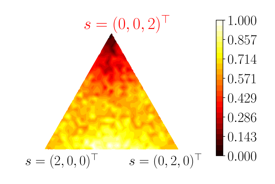
(a) $B=1$

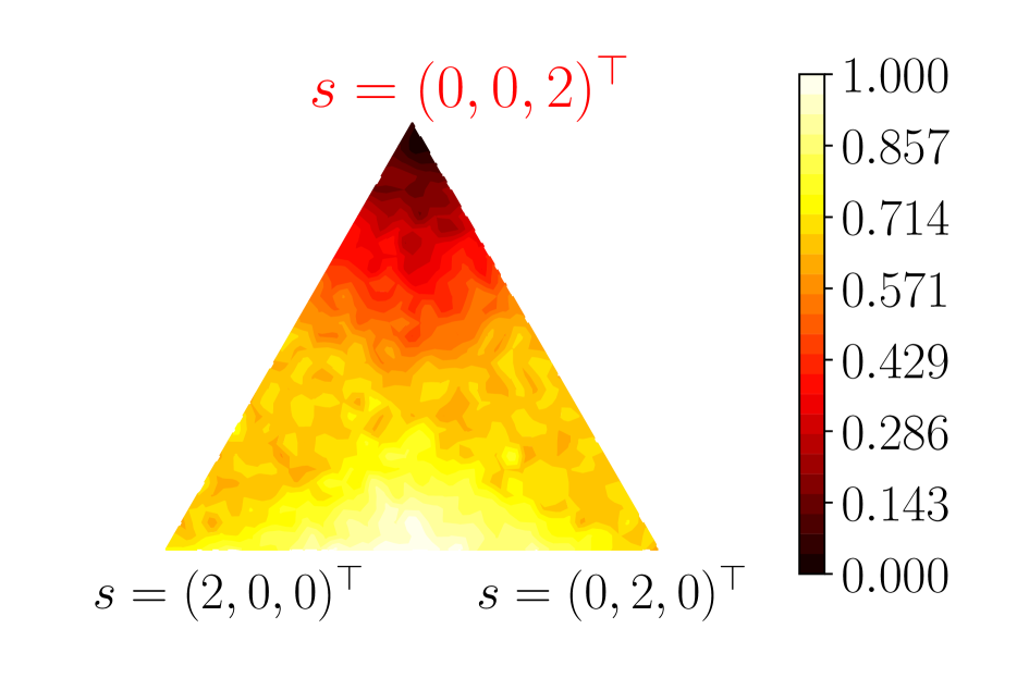
(b) $B=5$

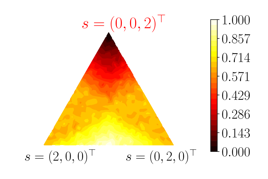
(c) $B=10$

(d) $B=50$

(e) $B=100$

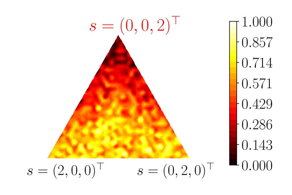
(f) $B=1$

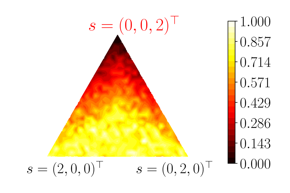
(g) $B=5$

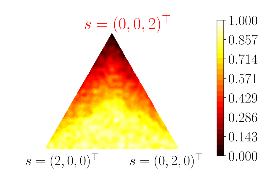
(h) $B=10$

(i) $B=50$

(j) $B=100$

Figure 4: Impact of the sampling parameter $B$ on the loss $\ell_{\text{Noised bal.}}^{K,1,B}$ (top part: $K=1$, bottom part: $K=2$)

Finally,  Figure 1(j) shows our noised imbalanced top-$K$ loss. Additional visualizations of our noised top-$K$ loss illustrating the effect of $B$ and $\epsilon$ can be found in the appendix, see Figures 4 and 5.

4 Experiments

The Pytorch (Paszke et al., 2019) code for our top-$K$ loss and experiments can be found at: https://github.com/garcinc/noised-topk.

4.1 Influence of $\epsilon$ and gradient sparsity

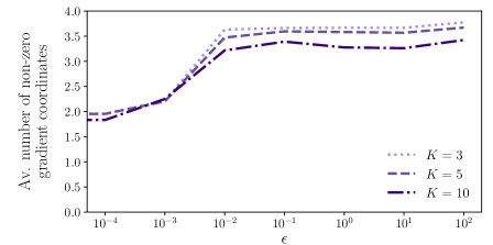
Figure 2: Average number of non-zero gradient coordinates as a function of $\epsilon$ (loss $\ell_{\text{Noised bal.}}^{K,\epsilon,3}$, CIFAR-100 dataset, DenseNet 40-40 model, 1st epoch). The gradient dimension is 100. We see that the gradient remains sparse even for large values of $\epsilon$. Together with Table 2, this shows that having a non-sparse gradient is not a necessary condition for successful learning, contrary to what is suggested in Berrada et al. (2018)

Table 2 shows the influence of $\epsilon$ on CIFAR-100 top-5 accuracy. When $\epsilon=0$, $\ell_{\text{Noised bal.}}^{K,\epsilon,B}$ coincides with $\ell_{\textrm{Cal. Hinge}}^{K}$. We see that a model trained with this loss fails to learn properly. This resonates with the observation made by Berrada et al. (2018) that a model trained with $\ell_{\textrm{Hinge}}^{K}$, which is close to $\ell_{\textrm{Cal. Hinge}}^{K}$, also fails to learn. Table 2 also shows that when $\epsilon$ is too small ($\epsilon=10^{-4}$ or $\epsilon=10^{-3}$), the optimization remains difficult and the learned models have very low performance. For sufficiently high values of $\epsilon$, in the order of $10^{-2}$ or greater, the smoothing is effective and the learned models achieve a very high top-5 accuracy. Table 2 also shows that although the optimal value of $\epsilon$ appears to be around $10^{-1}$, the optmization is robust to high values of $\epsilon$.

Berrada et al. (2018) argue that a reason a model trained with $\ell_{\textrm{Hinge}}^{K}$ fails to learn is because of the sparsity of the gradient of $\ell_{\textrm{Hinge}}^{K}$. Indeed, for any $\mathbf{s}\in\mathbb{R}^{L}$, $y\in[L]$, $\nabla_{s}\ell_{\textrm{Hinge}}^{K}(\mathbf{s},y)$ has at most two non-zero coordinates. This is one of the main reasons put forward by the authors to motivate the smoothing of $\ell_{\textrm{Hinge}}^{K}$ into $\ell_{\text{Smoothed Hinge}}^{K,\tau}$, whose gradient coordinates are all non-zero.

We investigate the behaviour of the gradient of our loss by computing $\nabla_{s}\ell_{\text{Noised bal.}}^{K,\epsilon,B}(\mathbf{s},y)$ for each training example during the first epoch. We then compute the average number of non-zero coordinates in the gradient. We repeat this process for several values of $\epsilon$ and report the results in Figure 2. There are two points to highlight:

$\bullet$ The number of non-zero gradients coordinates increases with $\epsilon$. This is consistent with our illustration example in Section 3.2: high values of $\epsilon$ allow putting weights on gradient coordinates whose score is close to the $\mathrm{top}_{K}$ score.

$\bullet$ Even when $\epsilon$ is large, the number of non-zero gradient coordinates is small: on average, 4 out of 100. In comparison, for $\ell^{K}_{\textrm{CE}}$ and $\ell_{\text{Smoothed Hinge}}^{K,\tau}$, all gradient coordinates are non-zero. Yet, even with such sparse gradient vectors, we manage to reach better top-5 accuracies than $\ell^{K}_{\textrm{CE}}$ and $\ell_{\text{Smoothed Hinge}}^{K,\tau}$ (see Table 4). Therefore, one of the main takeaway is that a non-sparse gradient does not appear to be a necessary condition for successful learning contrary to what is suggested in Berrada et al. (2018). A sufficiently high probability (controlled by $\epsilon$) that each coordinate is updated at training is enough to achieve good performance.

4.2 Influence of $B$

Table 3: Influence of $B$ hyper-parameter on the best validation top-5 accuracy (loss $\ell_{\text{Noised bal.}}^{5,0.2,B}$, CIFAR-100 dataset, DenseNet 40-40 model. The training procedure is the same as in Section 4.4.)

$B$	1	2	3	5	10	50	100
Top-5 acc	94.28	94.2	94.46	94.52	94.24	94.64	94.52

Table 3 shows the influence of the number of sampled standard normal random vectors $B$ on CIFAR-100 top-5 accuracy for a model trained with our balanced loss with $K=5$. $B$ appears to have little impact on top-5 accuracy, indicating that there is no need to precisely estimate the expectation in Equation 11. As increasing $B$ comes with computation overhead (see next section) and does not yield an increase of top-$K$ accuracy, we advise setting it to a small value (e.g., $3\leq B\leq 10)$.

4.3 Computation time

In Figure 3, we plot the average epoch duration of a model trained with the cross entropy $\ell_{\textrm{CE}}$, the loss from Berrada et al. (2018) $\ell_{\text{Smoothed Hinge}}^{K,\tau}$, and our balanced loss $\ell_{\text{Noised bal.}}^{K,\epsilon,B}$ (for several values of $B$) as a function of $K$. For standard training values, i.e., $K=5$, $B=3$, the average epoch time is 65s for $\ell_{\textrm{CE}}$, 68s for $\ell_{\text{Noised bal.}}^{K,\epsilon,B}$ (+4.6% w.r.t. $\ell_{\textrm{CE}}$) and 81s for $\ell_{\text{Smoothed Hinge}}^{K,\tau}$ (+24.6% w.r.t. $\ell_{\textrm{CE}}$). Figure 3 further shows that while the average epoch duration of $\ell_{\text{Smoothed Hinge}}^{K,\tau}$ seems to scale linearly in $K$, our loss does not incur an increased epoch duration when $K$ increases. Thus, for $K=10$, the average epoch time for $\ell_{\text{Smoothed Hinge}}^{K,\tau}$ is 90s versus 60s for $\ell_{\text{Noised bal.}}^{K,\epsilon,B}$ with $B=3$. While for most classical datasets Russakovsky et al. (2015); Krizhevsky (2009) small values of $K$ are enough to achieve high top-$K$ accuracy, for other applications high values of $K$ may be used (Covington et al., 2016; Cole et al., 2020), making our balanced loss computationally attractive.

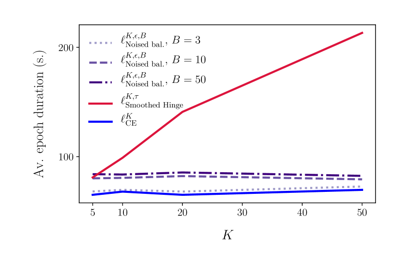
Figure 3: Average epoch time as a function of $K$ for different losses (CIFAR-100 dataset, DenseNet 40-40 model). The proposed loss $\ell_{\text{Noised bal.}}^{K,\epsilon,B}$ is not sensitive to the parameter $K$ contrarily to $\ell_{\text{Smoothed Hinge}}^{K,\tau}$ introduced by Berrada et al. (2018).

4.4 Comparisons for balanced classification

The CIFAR-100 Krizhevsky (2009) dataset contains 60,000 images (50,000 images in the training set and 10,000 images in the test set) categorized in 100 classes. The classes are grouped into 20 superclasses (e.g., fish, flowers, people), each regrouping 5 classes. Here we compare the top-$K$ accuracy of a deep learning model trained on CIFAR-100 with either our balanced loss $\ell_{\text{Noised bal.}}^{K,\epsilon,B}$, the cross entropy $\ell_{\textrm{CE}}$, or the loss from Berrada et al. (2018), $\ell_{\text{Smoothed Hinge}}^{K,\tau}$, which is the current state-of-the art top-$K$ loss for deep learning. We repeat the experiment from Section 5.1 of Berrada et al. (2018) to study how $\ell_{\text{Noised bal.}}^{K,\epsilon,B}$ reacts when noise is introduced in the labels. More precisely, for each training image, its label is sampled randomly within the same super-class with probability $p$. Thus, $p=0$ corresponds to the original dataset and $p=0.5$ corresponds to a dataset where all the training examples have a label corresponding to the right superclass, but half of them (on average) have a different label than the original one. With such a dataset, a perfect top-5 classifier is expected to have a $100\%$ top-5 accuracy. As in Berrada et al. (2018) we extract 5000 images from the training set to build a validation set. We use the same hyperparameters as Berrada et al. (2018): we train a DenseNet 40-40 Huang et al. (2017) for 300 epochs with SGD and a Nesterov momentum of 0.9. For the learning rate, our policy consists in starting with value of 0.1 and dividing it by ten at epoch 150 and 225. The batch size and weight decay are set to 64 and $1.10^{-4}$ respectively. Following Berrada et al. (2018), the smoothing parameter $\tau$ of $\smash{\ell_{\text{Smoothed Hinge}}^{K,\tau}}$ is set to 1.0. For $\ell_{\text{Noised bal.}}^{K,\epsilon,B}$, we set the noise parameter $\epsilon$ to 0.2 and the number of noise samples $B$ at 10. We keep the models with the best top-5 accuracies on the validation set and report the top-5 accuracy on the test set in Table 4. The results are averaged over four runs with four different random seeds (we give the 95% confidence inverval). They show that the models trained with $\ell_{\text{Noised bal.}}^{5,0.2,10}$ give the best top-5 accuracies except when $p=0.1$ where it is slightly below $\ell_{\text{Smoothed Hinge}}^{5,1.0}$. We also observe that the performance gain over the cross entropy is significant in the presence of label noise (i.e., for $p>0)$.

We provide additional experiments on ImageNet (Russakovsky et al., 2015) in Appendix D.

Table 4: Top-5 accuracy for different losses as a function of the label noise probability $p$ within the superclasses of CIFAR-100 (DenseNet 40-40 model).

Label noise $p$	$\ell^{K}_{\textrm{CE}}$	$\ell_{\text{Smoothed Hinge}}^{5,1.0}$	$\ell_{\text{Noised bal.}}^{5,0.2,10}$
0.0	$94.2{\pm}0.1$	$93.3{\pm}0.0$	$\mathbf{94.4}{\pm}0.1$
0.1	$90.3{\pm}0.2$	$\mathbf{92.2}{\pm}0.3$	$91.9{\pm}0.1$
0.2	$87.6{\pm}0.1$	$90.4{\pm}0.2$	$\mathbf{90.7}{\pm}0.5$
0.3	$85.7{\pm}0.4$	$88.8{\pm}0.1$	$\mathbf{89.7}{\pm}0.1$
0.4	$83.6{\pm}0.2$	$87.4{\pm}0.1$	$\mathbf{87.8}{\pm}0.6$

4.5 Comparison for imbalanced classification

4.5.1 Pl@ntNet-300K

Table 5: Macro-average top-$K$ accuracy (on test set) for different losses measured on Pl@ntNet-300K, a heavy-tailed dataset with high ambiguity (ResNet-50 model). The three numbers in parentheses represent respectively the mean top-$K$ accuracies of 1) few shot classes ($<20$ training images) 2) medium shot classes ($20\leq.\leq 100$ training images) 3) many shot classes ($>100$ training images).

K $\ell_{\textrm{CE}}$ $\ell_{\text{Smoothed Hinge}}^{K,0.1}$ $\ell_{\text{Noised bal.}}^{K,1.0,5}$ focal ($\gamma=2.0$) $\ell_{\textrm{LDAM}}^{\max m_{y}=0.2}$ $\ell_{\text{Noised imbal.}}^{K,0.01,5,\max m_{y}=0.2}$ 1 $36.3{\pm}0.3$ ($12.6$/$42.9$/$71.7$) $35.7{\pm}0.2$ ($13.1$/$41.5$/$71.1$) $35.8{\pm}0.3$ ($12.4$/$42.1$/$\mathbf{72.1}$) $37.6{\pm}0.3$ ($15.5$/$43.4$/$71.4$) $40.6{\pm}0.1$ ($20.9$/$45.8$/$71.2$) $\mathbf{42.4}{\pm}0.3$ ($\mathbf{23.9}$/$\mathbf{46.3}$/$72.1$) 3 $58.8{\pm}0.4$ ($32.4$/$\mathbf{75.3}$/$92.0$) $50.3{\pm}0.2$ ($16.7$/$69.8$/$\mathbf{92.7}$) $58.7{\pm}0.4$ ($32.2$/$73.8$/$88.8$) $60.4{\pm}0.3$ ($35.9$/$74.8$/$92.0$) $63.3{\pm}0.3$ ($43.0$/$74.1$/$90.0$) $\mathbf{64.9}{\pm}0.4$ ($\mathbf{44.8}$/$74.5$/$92.1$) 5 $68.7{\pm}0.2$ ($45.1$/$\mathbf{86.3}$/$95.4$) $50.9{\pm}0.3$ ($12.1$/$78.1$/$95.7$) $66.4{\pm}0.5$ ($42.0$/$82.5$/$95.5$) $69.7{\pm}0.2$ ($47.5$/$84.8$/$\mathbf{95.8}$) $71.9{\pm}0.3$ ($54.0$/$83.0$/$94.0$) $\mathbf{73.2}{\pm}0.5$ ($\mathbf{55.3}$/$84.2$/$95.3$)

Table 6: Top-$K$ accuracy (on test set) for different losses measured on ImageNet-LT (ResNet-34 model). The three numbers in parentheses represent respectively the mean top-$K$ accuracies of 1) few shot classes ($<20$ training images) 2) medium shot classes ($20\leq.\leq 100$ training images) 3) many shot classes ($>100$ training images).

K $\ell_{\textrm{CE}}$ $\ell_{\text{Smoothed Hinge}}^{K,0.1}$ focal ($\gamma=1.0$) $\ell_{\textrm{LDAM}}^{\max m_{y}=0.4}$ $\ell_{\text{Noised imbal.}}^{K,0.1,5,\max m_{y}=0.4}$ 1 $37.0{\pm}0.1$ ($1.5$/$28.2$/$60.6$) $37.3{\pm}0.1$ ($1.3$/$28.6$/$\mathbf{60.7}$) $37.7{\pm}0.0$ ($2.4$/$29.8$/$59.9$) $\mathbf{39.3}{\pm}0.2$ ($\mathbf{10.5}$/$\mathbf{33.1}$/$57.1$) $38.7{\pm}0.0$ ($7.6$/$32.3$/$57.6$) 3 $55.5{\pm}0.1$ ($8.2$/$53.0$/$\mathbf{75.3}$) $42.0{\pm}0.1$ ($0.0$/$29.1$/$72.9$) $56.2{\pm}0.0$ ($10.2$/$\mathbf{54.0}$/$75.1$) $56.0{\pm}0.2$ ($24.1$/$52.0$/$72.3$) $\mathbf{56.5}{\pm}0.1$ ($\mathbf{27.0}$/$52.6$/$71.7$) 5 $63.2{\pm}0.1$ ($15.8$/$63.1$/$80.1$) $39.0{\pm}0.1$ ($0.0$/$20.7$/$75.5$) $\mathbf{63.8}{\pm}0.1$ ($17.8$/$\mathbf{63.6}$/$\mathbf{80.3}$) $63.1{\pm}0.2$ ($32.9$/$60.1$/$77.7$) $63.5{\pm}0.1$ ($\mathbf{37.0}$/$60.2$/$77.0$)

We consider Pl@ntNet-300K, a dataset of plant images recently introduced in Garcin et al. (2021). It consists of 306,146 plant images distributed in 1,081 species (the classes). The particularities of the dataset are its long-tailed distribution (80% of the species with the least number of images account for only 11% of the total number of images) and the class ambiguity: many species are visually similar. For such an imbalanced dataset, accuracy and top-$K$ accuracy mainly reflect the performance of the model on the few classes representing the vast majority of images. Often times, we also want the model to yield satisfactory results on the classes with few images. Therefore, for this dataset we report macro-average top-$K$ accuracy, which is obtained by computing top-$K$ accuracy for each class separately and then taking the average over classes. Thus, the class with only a few images contributes the same as the class with thousands of images to the overall result.

In this section we compare the macro-average top-$K$ accuracy of a deep neural network trained with either $\smash{\ell_{\textrm{CE}},\ell_{\text{Smoothed Hinge}}^{K,\tau},\ell_{\text{Noised bal.}}^{K,\epsilon,B},\ell_{\text{Noised imbal.}}^{K,\epsilon,B,m_{y}}}$ and $\smash{\ell_{\textrm{LDAM}}^{m_{y}}}$, the loss from Cao et al. (2019) based on uneven margins providing state-of-the-art performance in Fine-Grained Visual Categorization tasks.

Setup: We train a ResNet-50 He et al. (2016) pre-trained on ImageNet Russakovsky et al. (2015) for 30 epochs with SGD with a momentum of 0.9 with the Nesterov acceleration. We use a learning rate of $2.10^{-3}$ divided by ten at epoch 20 and epoch 25. The batch size and weight decay are set to 32 and $1.10^{-4}$ respectively. The smoothing parameter $\tau$ for $\smash{\ell_{\text{Smoothed Hinge}}^{K,\tau}}$ is set to 0.1.

To tune the margins of $\smash{\ell_{\textrm{LDAM}}^{m_{y}}}$ and $\ell_{\text{Noised imbal.}}^{K,\epsilon,B,m_{y}}$ more easily, we follow Wang et al. (2018); Cao et al. (2019): we normalize the last hidden activation and the weight vectors of the last fully-connected layer to both have unit $\ell_{2}$-norm, and we multiply the scores by a scaling constant, tuned for both losses on the validation set, leading to 40 for $\smash{\ell_{\textrm{LDAM}}^{m_{y}}}$ and 60 for $\smash{\ell_{\text{Noised imbal.}}^{K,\epsilon,B,m_{y}}}$.

Finally, we tune the constant $C$ by tuning the largest margin $\max_{y\in[L]}m_{y}$ for both $\smash{\ell_{\textrm{LDAM}}^{m_{y}}}$ and $\ell_{\text{Noised imbal.}}^{K,\epsilon,B,m_{y}}$. We find that for both losses, the optimal largest margin is 0.2. For $\smash{\ell_{\text{Noised imbal.}}^{K,\epsilon,B,m_{y}}}$, we set $\epsilon=10^{-2}$ and $B=5$. We further discuss hyperparameter tuning in Appendix E.

We train the network with the top-$K$ losses $\smash{\ell_{\text{Smoothed Hinge}}^{K,\tau},\ell_{\text{Noised bal.}}^{K,\epsilon,B}}$ and $\smash{\ell_{\text{Noised imbal.}}^{K,\epsilon,B,m_{y}}}$ for $K\in\{1,3,5\}$. For all losses, we perform early stopping based on the best macro-average top-$K$ accuracy on the validation set (for $K\in\{1,3,5\}$). We report the results on the test set in Table 5 (three seeds, 95% confidence interval). We find that the loss from Berrada et al. (2018) fails to generalize to the tail classes in such an imbalanced setting. In contrast, $\ell_{\text{Noised bal.}}^{K,\epsilon,B}$ gives results similar to the cross-entropy while $\ell_{\text{Noised imbal.}}^{K,\epsilon,B,m_{y}}$ provides the best results (regardless of the value of $K$). Noticeably, it outperforms $\smash{\ell_{\textrm{LDAM}}^{m_{y}}}$ (Cao et al., 2019) for all cases.

4.5.2 ImageNet-LT

We test $\ell_{\text{Noised imbal.}}^{K,\epsilon,B,m_{y}}$ on ImageNet-LT (Liu et al., 2019), a dataset of 115,836 training images obtained by subsampling images from ImageNet with a pareto distribution. The resulting class imbalance is much less pronounced than for Pl@ntNet-300K.

We train a ResNet34 with several losses for $K\in\{1,3,5\}$ for 100 epochs with a learning rate of $1.10^{-2}$ divided by 10 at epoch 60 and 80. We use a batch size of 128 and set the weight decay to $2.10^{-3}$. All hyperparameters are tuned on the 20,000 images validation set from Liu et al. (2019). The results on the test set (four seeds, 95% confidence interval) are reported in Table 6. They show that $\ell_{\text{Noised Imbal.}}^{K,\epsilon,B,m_{y}}$ performs very well on few shot classes compared to the other losses. Since ImageNet-LT is much less imbalanced than Pl@ntNet-300K, there are fewer such classes, hence the overall gain is less salient than for Pl@ntNet-300K.

5 Conclusion and perspectives

We propose a novel top-$K$ loss as a smoothed version of the top-$K$ calibrated hinge loss of Yang & Koyejo (2020). Our loss function is well suited for training deep neural networks, contrarily to the original top-$K$ calibrated hinge loss (e.g., the poor performance of the case $\epsilon=0$ in Table 2, that reduces to their loss). The smoothing procedure we propose applies the perturbed optimizers framework to smooth the top-$K$ operator. We show that our loss performs well compared to the current state-of-the-art top-$K$ losses for deep learning while being significantly faster to train when $K$ increases. At training, the gradient of our loss w.r.t. the score is sparse, showing that non-sparse gradients are not necessary for successful learning. Finally, a slight adaptation of our loss for imbalanced datasets (leveraging uneven margins) outperforms other baseline losses. Studying deep learning optimization methods for other set-valued classification tasks, such as average size control or point-wise error control Chzhen et al. (2021) are left for future work.

Appendix A Reminder on Top-$K$ calibration

Here we provide some elements introduced by Yang & Koyejo (2020) on top-$K$ calibration.

Definition A.1.

(Yang & Koyejo, 2020, Definition 2.3). For a fixed $K\in[L]$, and given $\mathbf{y}\in\mathbb{R}^{L}$ and $\tilde{\mathbf{y}}\in\mathbb{R}^{L}$, we say that $\mathbf{y}$ is top-$K$ preserving w.r.t. $\tilde{\mathbf{y}}$, denoted $P_{K}(\mathbf{y},\tilde{\mathbf{y}})$, if for all $k\in[L]$,

$$\tilde{y}_{k}>\mathrm{top}_{K+1}(\tilde{\mathbf{y}}) \implies{y}_{k}>\mathrm{top}_{K+1}({\mathbf{y}})$$ (14)

$$\tilde{y}_{k}<\mathrm{top}_{K}(\tilde{\mathbf{y}}) \implies y_{k}<\mathrm{top}_{K}({\mathbf{y}})\enspace.$$ (15)

The negation of this statement is $\neg P_{k}(\mathbf{y},\tilde{\mathbf{y}})$.

We let $\Delta_{L}\triangleq\{\boldsymbol{\pi}\in\mathbb{R}^{L}:\sum_{k\in[L]}\pi_{k}=1,\pi_{k}\geq 0\}$ denote the probability simplex of size $L$. For a score $\mathbf{s}\in\mathbb{R}^{L}$ and $\boldsymbol{\pi}\in\Delta_{L}$ representing the conditional distribution of $y$ given $x$, we write the conditional risk at $x\in\mathcal{X}$ as $\mathcal{R}_{\ell|x}(\mathbf{s},\boldsymbol{\pi})=\mathbb{E}_{y|x\sim\pi}(\ell(\mathbf{s},y))$ and the (integrated) risk as $\mathcal{R}_{\ell}(f)\triangleq\mathbb{E}_{(x,y)\sim\mathbb{P}}[\ell(f(x),y)]$ for a scoring function $f:\mathcal{X}\to\mathbb{R}^{L}$. The associated Bayes risks are defined respectively by $\mathcal{R}_{\ell|x}^{*}(\boldsymbol{\pi})\triangleq\inf_{\mathbf{s}\in\mathbb{R}^{L}}\mathcal{R}_{\ell|x}(\mathbf{s},\boldsymbol{\pi})$ (respectively by $\mathcal{R}_{\ell}^{*}\triangleq\inf_{f:\mathcal{X}\to\mathbb{R}^{L}}\mathcal{R}_{\ell}(f)$) .

Definition A.2.

(Yang & Koyejo, 2020, Definition 2.4). A loss function $\ell:\mathbb{R}^{L}\times\mathcal{Y}\rightarrow\mathbb{R}$ is top-$K$ calibrated if for all $\boldsymbol{\pi}\in\Delta_{L}$ and all $x\in\mathcal{X}$:

$$\inf_{\mathbf{s}\in\mathbb{R}^{L}:\neg P_{k}(\mathbf{s},\boldsymbol{\pi})}\mathcal{R}_{\ell|x}(\mathbf{s},\boldsymbol{\pi})\!>\mathcal{R}_{\ell|x}^{*}(\boldsymbol{\pi})\enspace.$$ (16)

In other words, a loss is calibrated if the infimum can only be attained among top-$K$ preserving vectors w.r.t. the conditional probability distribution.

Theorem A.3.

Suppose $\ell$ is a nonnegative top-$K$ calibrated loss function. Then $\ell$ is top-$K$ consistent, i.e., for any sequence of measurable functions $f^{(n)}:\mathcal{X}\rightarrow\mathbb{R}^{L}$, we have:

$$\mathcal{R}_{\ell}\left(f^{(n)}\right)\rightarrow\mathcal{R}_{\ell}^{*}\Longrightarrow\mathcal{R}_{\ell^{K}}\left(f^{(n)}\right)\rightarrow\mathcal{R}_{\ell^{K}}^{*}\enspace.$$

In their paper, Yang & Koyejo (2020) propose a slight modification of the multi-class hinge loss $\ell_{\textrm{Hinge}}^{K}$ and show that it is top-$K$ calibrated:

$$\ell_{\textrm{Cal.~{}Hinge}}^{K}(\mathbf{s},y)=(1+\mathrm{top}_{K+1}(\mathbf{s})-s_{y})_{+}\enspace.$$ (17)

Appendix B Proofs and technical lemmas

B.1 Proof of Proposition 3.3

Proof.

We define $\smash{\mathcal{C}_{K}\triangleq\left\{\mathbf{z}\in\mathbb{R}^{L},\sum_{k\in[L]}z_{k}=K,0\leq z_{k}\leq 1,\>\forall k\in[L]\right\}}$. For $\mathbf{s}\in\mathbb{R}^{L}$, one can check that $\mathrm{arg\,top}\Sigma_{K}(\mathbf{s})=\mathop{\mathrm{arg\,max}}_{\mathbf{z}\in\mathcal{C}_{K}}\langle\mathbf{z},\mathbf{s}\rangle$. Recall that $Z$ is a standard normal random vector, i.e., $Z\sim\mathcal{N}(0,\operatorname{Id}_{L})$.

• $\mathcal{C}_{K}$ is a convex polytope and the multivariate normal has positive differentiable density. So, we can apply (Berthet et al., 2020, Proposition 2.2). For that, it remains to determine the constant $R_{\mathcal{C}_{K}}$ and $M_{\mu}$. First, $R_{\mathcal{C}_{K}}\triangleq\max_{\mathbf{z}\in\mathcal{C}_{K}}\left\lVert\mathbf{z}\right\rVert$. For simplicity, let us compute $\max_{\mathbf{z}\in\mathcal{C}_{K}}\left\lVert\mathbf{z}\right\rVert^{2}$, i.e.,

  $$\max\left\lVert\mathbf{z}\right\rVert^{2}$$ (18)

  $$\mathrm{s.t.}~{}\sum_{k\in[L]}z_{k}=K,\,\forall k\in[L],z_{k}\in[0,1].$$ (19)

  Note that this corresponds to the well known quadratic knapsack problem. A numerical solution can be obtained, see for instance Helgason et al. (1980). To obtain our bound, note that for $z\in\mathcal{C}_{K}$ one can check that

  $$\left\lVert\mathbf{z}\right\rVert^{2}= \sum_{k\in[L]}z_{k}^{2}\leq\sum_{k\in[L]}z_{k}\quad(\text{since }\,\forall k\in[L],z_{k}\in[0,1]).$$

  Hence, we have $\forall\mathbf{z}\in\mathcal{C}_{K},\left\lVert\mathbf{z}\right\rVert^{2}\leq K$. Now, one can check that this equality is achieved when choosing $\mathbf{z}=(1,\dots,1,0,\dots,0)^{\top}\in\mathbb{R}^{L}$ with $K$ non-zeros values, yielding $\max_{\mathbf{z}\in\mathcal{C}_{K}}\left\lVert\mathbf{z}\right\rVert=\sqrt{K}$. Following (Berthet et al., 2020, Proposition 2.2) this guarantees that $\mathrm{top}\Sigma_{K,\epsilon}$ is $\sqrt{K}$-Lipschitz.

  Let us show now that $M_{\mu}\triangleq\sqrt{\mathbb{E}_{Z}[\left\lVert\nabla_{Z}\nu(Z)\right\rVert^{2}]}=\sqrt{L}$ with $\nu(Z)=\frac{1}{2}\left\lVert Z\right\rVert^{2}$ and $Z\sim\mathcal{N}(0,\operatorname{Id}_{L})$. Hence, $M_{\mu}$ can be computed as:

  $$M_{\mu} =\sqrt{\mathbb{E}_{Z}\left[\left\lVert\nabla_{Z}\nu(Z)\right\rVert^{2}\right]}$$

  $$=\sqrt{\mathbb{E}_{Z}\left[\left\lVert Z\right\rVert^{2}\right]}$$

  $$=\sqrt{L}\enspace,$$

  where the last equality comes from $Z\sim\mathcal{N}(0,\operatorname{Id}_{L})$. Following (Berthet et al., 2020, Proposition 2.2) this guarantees that $\nabla\mathrm{top}\Sigma_{K,\epsilon}$ is $\tfrac{\sqrt{KL}}{\epsilon}$-Lipschitz.

• The last bullet of our proposition comes derives now directly from of (Berthet et al., 2020, Proposition 2.3).

∎

B.2 Proof of Proposition 3.5

Proof.

• From the triangle inequality and Proposition 3.3 we get for any $\mathbf{s},\mathbf{s}^{\prime}\in\mathbb{R}^{L}$:

  $$\left\lVert\nabla\mathrm{top}_{K,\epsilon}(\mathbf{s})-\nabla\mathrm{top}_{K,\epsilon}(\mathbf{s}^{\prime})\right\rVert =\lVert\left[\nabla\mathrm{top}\Sigma_{K,\epsilon}(\mathbf{s})-\nabla\mathrm{top}\Sigma_{K,\epsilon}(\mathbf{s}^{\prime})\right]-\left[\nabla\mathrm{top}\Sigma_{K-1,\epsilon}(\mathbf{s})-\nabla\mathrm{top}\Sigma_{K-1,\epsilon}(\mathbf{s}^{\prime})\right]\rVert$$

  $$\leq\lVert\nabla\mathrm{top}\Sigma_{K,\epsilon}(\mathbf{s})-\nabla\mathrm{top}\Sigma_{K,\epsilon}(\mathbf{s}^{\prime})\rVert+\lVert\nabla\mathrm{top}\Sigma_{K-1,\epsilon}(\mathbf{s})-\nabla\mathrm{top}\Sigma_{K-1,\epsilon}(\mathbf{s}^{\prime})\rVert$$

  $$\leq\left(2\frac{\sqrt{KL}}{\epsilon}+2\frac{\sqrt{(K-1)L}}{\epsilon}\right)\left\lVert\mathbf{s}-\mathbf{s}^{\prime}\right\rVert\leq 4\frac{\sqrt{KL}}{\epsilon}\left\lVert\mathbf{s}-\mathbf{s}^{\prime}\right\rVert$$

• Using the notation from (Berthet et al., 2020, Appendix A), with $F(\mathbf{s})=\mathrm{top}\Sigma_{K}(\mathbf{s})$ and $F_{\epsilon}(\mathbf{s})=\mathrm{top}\Sigma_{K,\epsilon}(\mathbf{s})$, we get the following bounds:

  $$0\leq\mathrm{top}\Sigma_{K,\epsilon}(\mathbf{s})-\mathrm{top}\Sigma_{K}(\mathbf{s})\leq\epsilon\cdot\mathrm{top}\Sigma_{K,1}(\mathbf{0})$$ (20)

  $$0\leq\mathrm{top}\Sigma_{K-1,\epsilon}(\mathbf{s})-\mathrm{top}\Sigma_{K-1}(\mathbf{s})\leq\epsilon\cdot\mathrm{top}\Sigma_{K-1,1}(\mathbf{0})\enspace.$$ (21)

  Additionally, using the maximal inequality for i.i.d. Gaussian variables, see for instance (Boucheron et al., 2013, Section 2.5), leads to:

  $$\mathrm{top}\Sigma_{K,1}(\mathbf{0})=\mathbb{E}\left[\sum_{k\in[K]}Z_{(k)}\right]\leq K\mathbb{E}\big{[}Z_{(1)}\big{]}\leq K\sqrt{2\log L}$$

  Subtracting (21) to (20), and reminding that $\mathrm{top}_{K}(\mathbf{s})=\mathrm{top}\Sigma_{K}(\mathbf{s})-\mathrm{top}\Sigma_{K-1}(\mathbf{s})$ (and similarly $\mathrm{top}_{K,\epsilon}(\mathbf{s})=\mathrm{top}\Sigma_{K,\epsilon}(\mathbf{s})-\mathrm{top}\Sigma_{K-1,\epsilon}(\mathbf{s})$) gives:

  $$-\epsilon\cdot(K-1)\sqrt{2\log L}\leq\mathrm{top}_{K,\epsilon}(\mathbf{s})-\mathrm{top}_{K}(\mathbf{s}) \leq\epsilon\cdot K\sqrt{2\log L}\enspace,$$

  thus leading to:

  $$\lvert\mathrm{top}_{K,\epsilon}(\mathbf{s})-\mathrm{top}_{K}(\mathbf{s})\rvert\leq\epsilon\cdot C_{K,L}\enspace,$$ (22)

  with $C_{K,L}=K\sqrt{2\log L}$.

∎

B.3 Proof of Proposition 3.7

Proof.

• First, note that $\mathbf{s}\mapsto\ell_{\text{Noised bal.}}^{K,\epsilon}(\mathbf{s},y)$ is continuous as a composition and sum of continuous functions. It is differentiable wherever $\psi:\mathbf{s}\mapsto 1+\mathrm{top}_{K+1,\epsilon}(\mathbf{s})-s_{y}$ is non-zero. From Definition 3.4 and Proposition 3.3 we get $\nabla_{s}\psi(\mathbf{s})=\mathbb{E}[\mathrm{arg\,top}\Sigma_{K+1}(\mathbf{s}+\epsilon Z)]-\delta_{y}$. The formula of the gradient follows from the chain rule.

∎

Appendix C Illustrations of the various losses encountered

In Figures 6 and 1, we provide a visualization of the loss landscapes for respectively $K=1$ and $K=2$ with $L=3$ labels. With $L=3$ labels, we display the visualization as level-sets restricted to a rescaled simplex: $2\dots\Delta_{3}$. Moreover, we have min/max rescaled all the losses so that they fully range the interval $[0,1]$. Note that as we are mainly interested in minimizing the losses, this post-processing would not modify the learned classifiers.

We provide also two additional figures illustrating the impact on our loss of the two main parameters: $\epsilon$ and $B$.

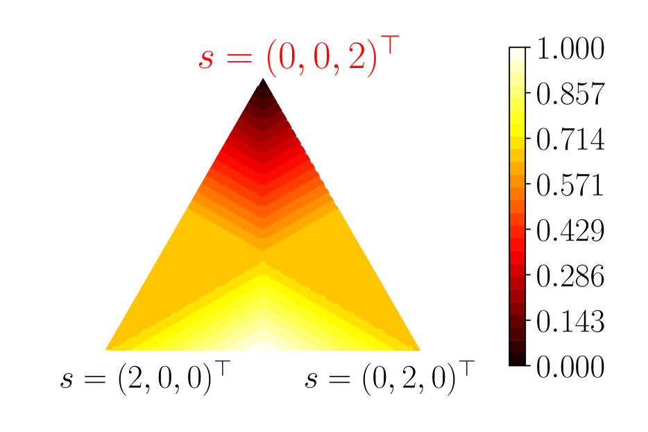
(a) $\epsilon=0.01$

(b) $\epsilon=0.1$

(c) $\epsilon=1$

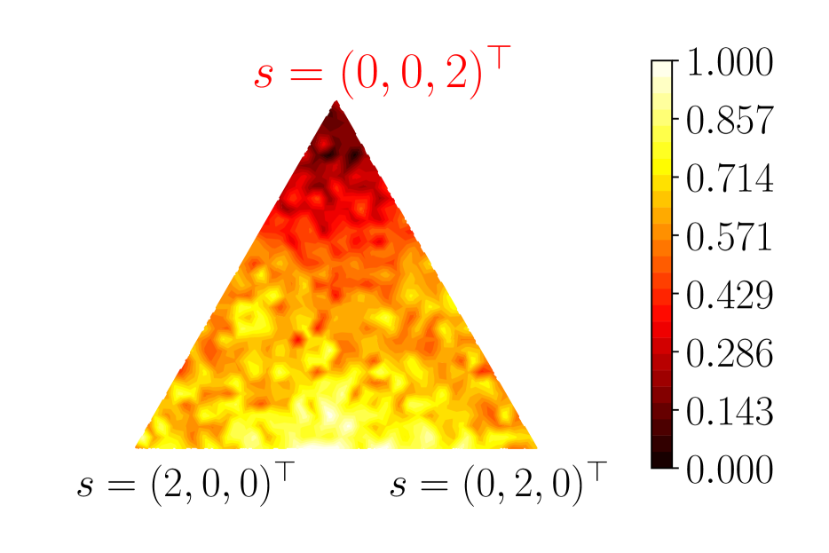
(d) $\epsilon=10$

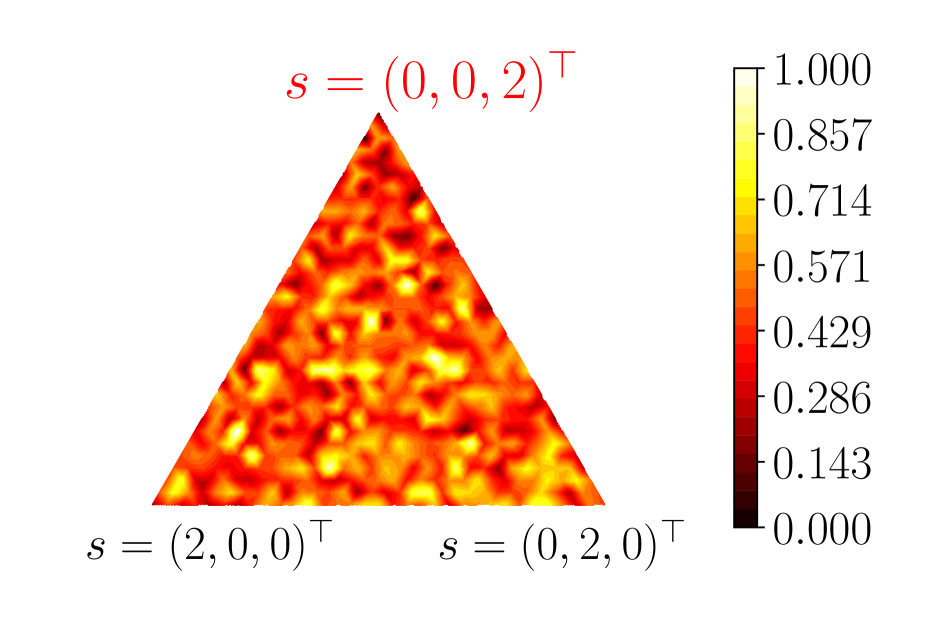
(e) $\epsilon=100$

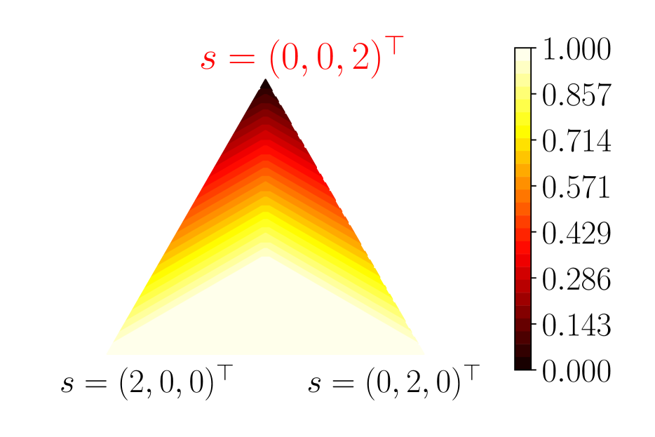
(f) $\epsilon=0.01$

(g) $\epsilon=0.1$

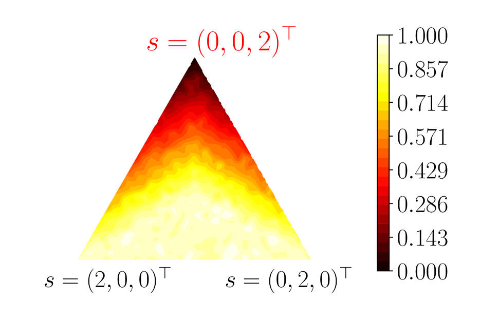
(h) $\epsilon=1$

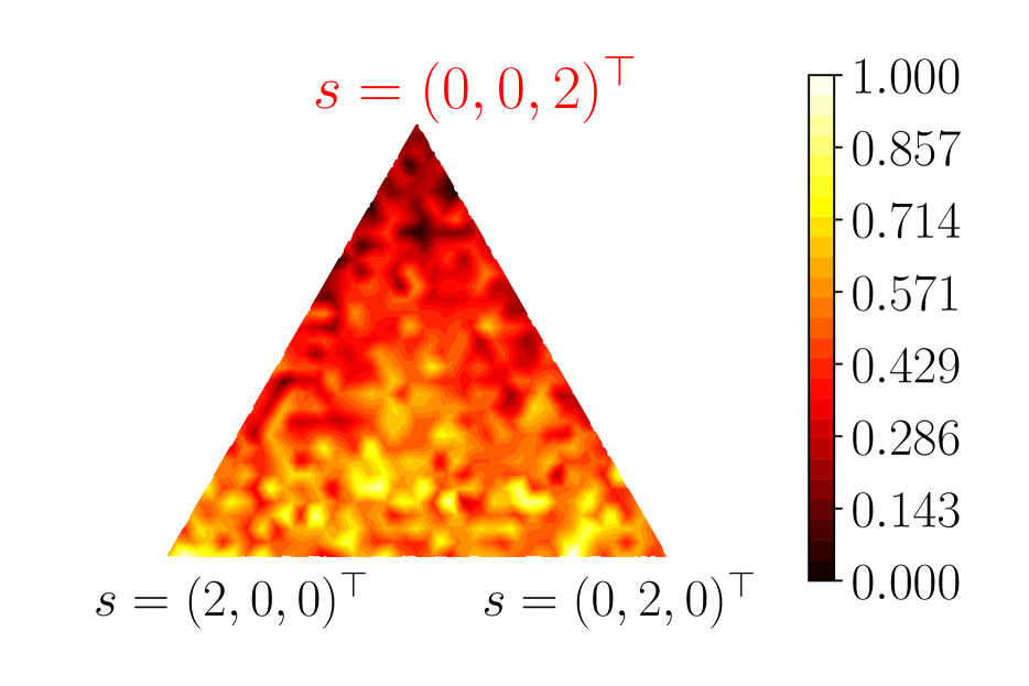
(i) $\epsilon=10$

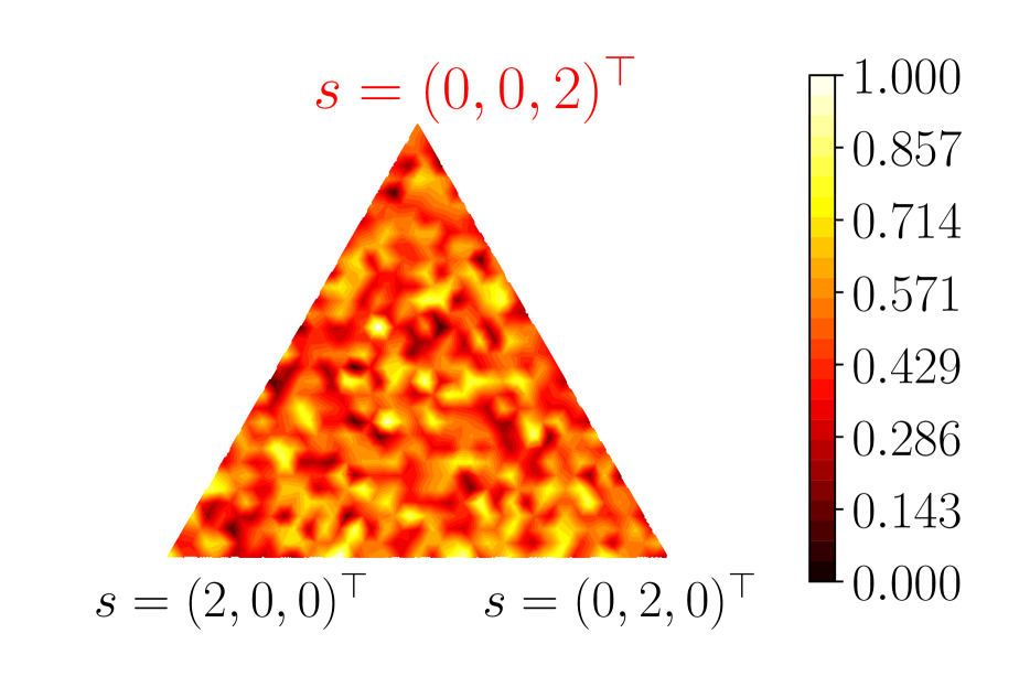
(j) $\epsilon=100$

Figure 5: Impact of the smoothing parameter $\epsilon$ on the loss $\ell_{\text{Noised bal.}}^{K,\epsilon,50}$ (top part: $K=1$, bottom part: $K=2$)

(a) Top-$K$:
$\ell=\ell^{K}$.$\ell_{\textrm{Cal.~{}Hinge}}^{K}$

(b) Cross-entropy:
$\ell=\ell_{\textrm{CE}}$.$\ell=\ell_{\textrm{Cal.~{}Hinge}}^{K}$

(c) Multi-class hinge:
$\ell=\ell_{\textrm{Hinge}}^{K}$.

(d) Calibrated hinge:
$\ell=\ell_{\textrm{Cal.~{}Hinge}}^{K}$.

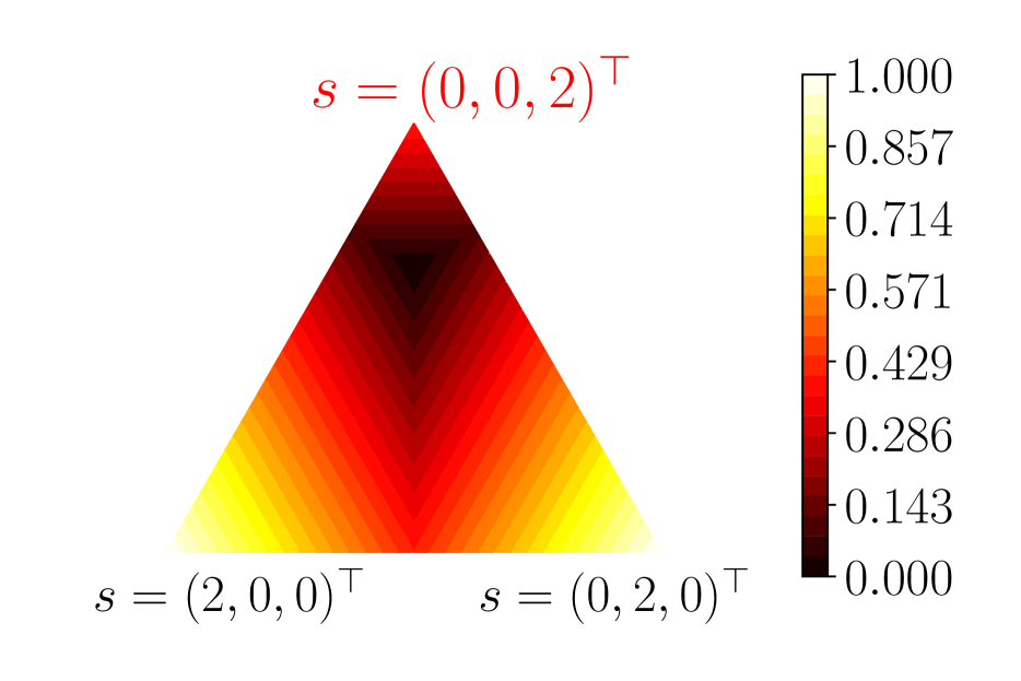
(e) Convexified hinge:
$\ell=\ell_{\textrm{CVXHinge}}^{K}$.

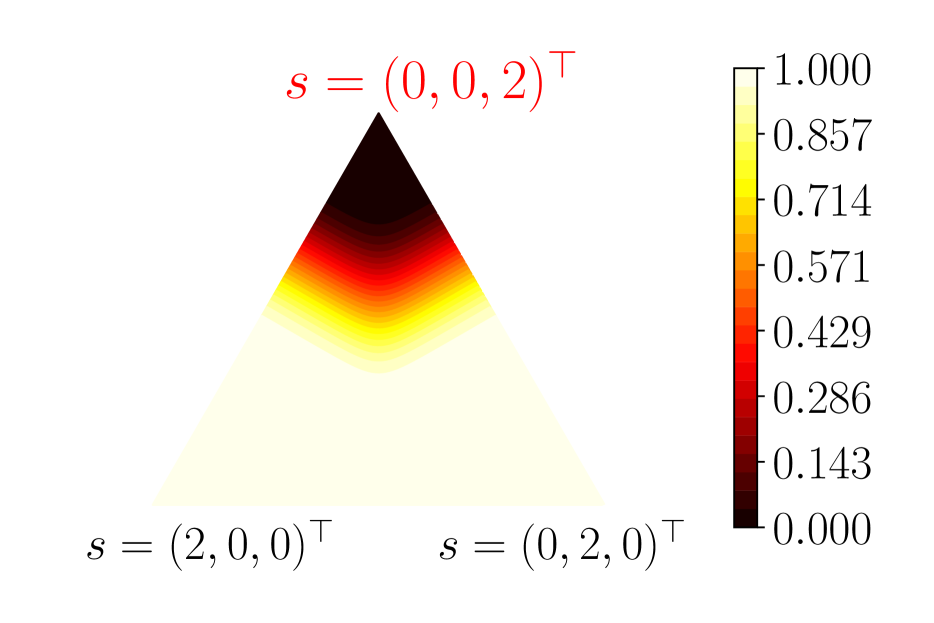
(f) Smoothed hinge
$\ell_{\text{Smoothed Hinge}}^{K,0.1}$.

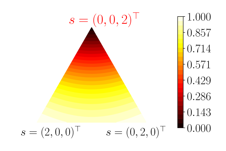
(g) Smoothed hinge
$\ell_{\text{Smoothed Hinge}}^{K,1}$.

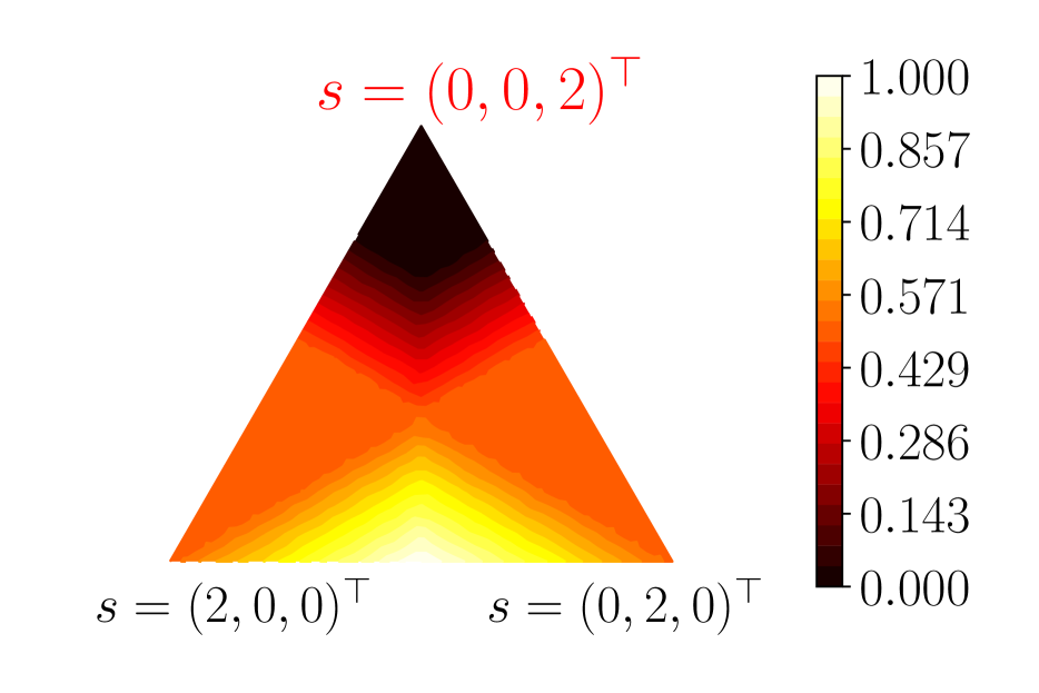
(h) Noised balanced: g
$\ell_{\text{Noised bal.}}^{K,0.3,30}$.$\ell_{\text{Smoothed Hinge}}^{K,0.4}$

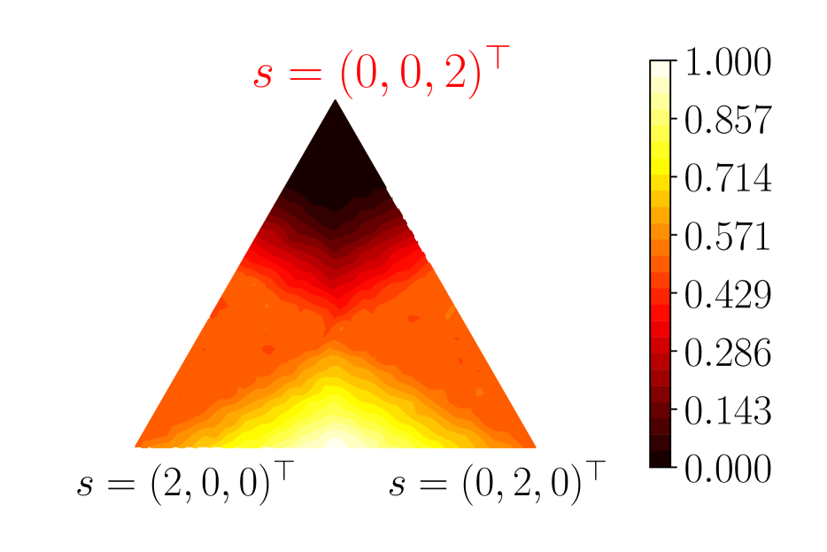
(i) Noised balanced:g
$\ell_{\text{Noised bal.}}^{K,1,30}$.$\ell_{\text{Smoothed Hinge}}^{K,0.4}$

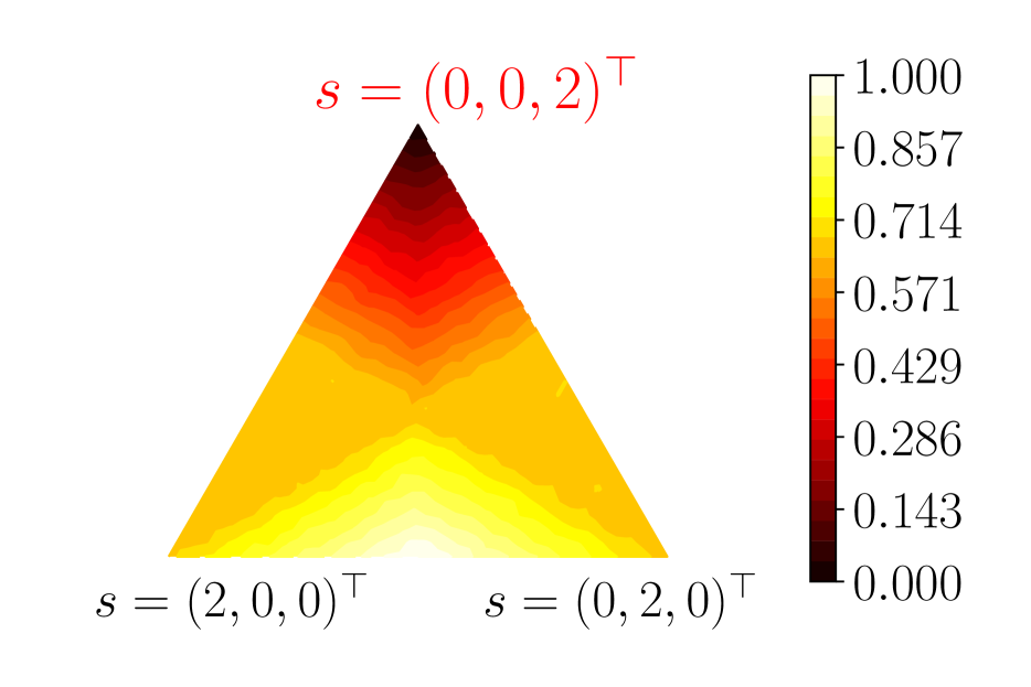
(j) Noised imbalanced:g
$\ell_{\text{Noised imbal.}}^{K,1,30,5}$.$\ell_{\text{Smoothed Hinge}}^{K,0.4}$

Figure 6: Level sets of the function $\mathbf{s}\mapsto\ell(\mathbf{s},y)$ for different losses described in Table 1, for $L=3$ classes, $K=1$ and a true label $y=2$ (corresponding to the upper corner of the triangles). For visualization the loss are rescaled between 0 and 1, and the level sets are restricted to vector $\mathbf{s}\in 2\cdot\Delta_{3}$. The losses have been harmonized to display a margin equal to 1. For our proposed loss, we have averaged the level sets over 100 replications to avoid meshing artifacts.

Appendix D Additional experiments

Table 7: top-1 accuracy cifar100

Label noise	$\ell^{K}_{\textrm{CE}}$	$\ell_{\text{Smoothed Hinge}}^{5,1.0}$	$\ell_{\text{Noised bal.}}^{5,0.2,10}$
0.0	$\mathbf{76.6}{\pm}0.1$	$69.2{\pm}0.1$	$68.7{\pm}0.3$
0.1	$71.0{\pm}0.2$	$\mathbf{71.2}{\pm}0.4$	$68.3{\pm}0.5$
0.2	$68.1{\pm}0.1$	$\mathbf{71.3}{\pm}0.3$	$69.4{\pm}0.5$
0.3	$65.5{\pm}0.3$	$\mathbf{70.8}{\pm}0.6$	$69.3{\pm}0.3$
0.4	$61.8{\pm}0.4$	$\mathbf{70.6}{\pm}0.2$	$69.1{\pm}0.4$

CIFAR-100: Table 7 reports the top-1 accuracy obtained by the models corresponding to the results of Table 4. Hence, we show here a misspecified case: we optimized our balanced loss for $K=5$, seeking to optimize top-5 accuracy, which is reported in Table 4, but report top-1 information. Table 7 shows that when there is no label noise, as expected cross entropy gives better top-1 accuracy than our top-5 loss. When the label noise is high, however, our loss leads to better top-1 accuracy.

Pl@ntNet-300K: Table 8 reports the top-$K$ accuracy obtained by the models corresponding to the results of Table 5. The top-$K$ accuracies are much higher than the macro-average top-$K$ accuracies reported in Table 5 because of the long-tailed distribution of Pl@ntNet-300K. The models perform well on classes with a lot of examples which leads to high top-$K$ accuracy. However, they struggle on classes with a small number of examples (which is the majority of classes, see Garcin et al. (2021)). Thus, for Pl@ntNet-300K top-$K$ accuracy is not very relevant as it mainly reflects the performance of the few classes with a lot of images, ignoring the performance on challenging classes (the one with few labels) Affouard et al. (2017). We report it for completeness and make a few comments:

Table 8: regular top-$K$ accuracy corresponding to the models in Table 5

K	$\ell_{\textrm{CE}}$	$\ell_{\text{Smoothed Hinge}}^{K,\tau}$	$\ell_{\text{Noised bal.}}^{K,\epsilon,B}$	focal	LDAM	$\ell_{\text{Noised imbal.}}^{K,\epsilon,B,m_{y}}$
1	$80.1{\pm}0.1$	$79.8{\pm}0.0$	$80.8{\pm}0.1$	$79.8{\pm}0.1$	$79.6{\pm}0.1$	$\mathbf{81.0}{\pm}0.1$
3	$93.1{\pm}0.0$	$93.2{\pm}0.0$	$\mathbf{93.5}{\pm}0.1$	$93.5{\pm}0.0$	$92.3{\pm}0.1$	$93.5{\pm}0.1$
5	$95.7{\pm}0.0$	$95.0{\pm}0.1$	$95.8{\pm}0.0$	$\mathbf{96.0}{\pm}0.0$	$95.2{\pm}0.2$	$95.8{\pm}0.1$
10	$97.5{\pm}0.0$	$95.5{\pm}0.0$	$97.5{\pm}0.0$	$\mathbf{97.7}{\pm}0.0$	$97.2{\pm}0.1$	$97.5{\pm}0.0$

First, our balanced noise loss gives better top-$K$ accuracies than the cross entropy or the loss from Berrada et al. (2018) for all $K$. Then, $\ell_{\text{Noised imbal.}}^{K,\epsilon,B,m_{y}}$ and $\ell_{\text{Noised bal.}}^{K,\epsilon,B}$ produce the best top-1 accuracy, respectively 81.0 and 80.8.

However, we insist that in such an imbalanced setting the macro-average top-$K$ accuracy reported in Table 5 is much more informative than regular top-$K$ accuracy. We see significant differences between the losses in Table 5 which are hidden in Table 8 because of the extreme class imbalance.

ImageNet: We test $\ell_{\text{Noised bal.}}^{K,\epsilon,B}$ on ImageNet. We follow the same procedure as Berrada et al. (2018): we train a ResNet-18 with SGD for 120 epochs with a batch size of 120 epochs. The learning rate is decayed by ten at epoch 30, 60 and 90. For $\ell_{\text{Smoothed Hinge}}^{K,\tau}$, the smoothing parameter $\tau$ is set to 0.1, the weight decay parameter to 0.000025 and the initial learning rate to 1.0, as in Berrada et al. (2018). For $\ell_{\textrm{CE}}$, the weight decay parameter is set to 0.0001 and the initial learning rate to 0.1, following Berrada et al. (2018). For $\ell_{\text{Noised bal.}}^{K,\epsilon,B}$, we use the same validation set as in Berrada et al. (2018) to set $\epsilon$ to 0.5, the weight decay parameter to 0.00015 and the initial learning rate to 0.1. $B$ is set to 10. We optimize all losses for $K=1$ and $K=5$. We perform early stopping based on best top-$K$ accuracy on the validation set and report the results on the test set (the official validation set of ImageNet) in Table 9 (3 seeds, 95% confidence interval). In the presence of low label noise, with an important number of training examples per class and for a nearly balanced dataset, all three losses give similar results. This is in contrast with Table 4 and Table 5, where significant differences appear between the different losses in the context of label noise or class imbalance.

Table 9: ImageNet test top-$K$ accuracy, ResNet-18.

K	$\ell_{\textrm{CE}}$	$\ell_{\text{Smoothed Hinge}}^{K,0.1}$	$\ell_{\text{Noised bal.}}^{K,0.5,10}$
1	$72.24{\pm}0.15$	$71.43{\pm}0.14$	$\mathbf{72.46}{\pm}0.15$
5	$90.60{\pm}0.05$	$\mathbf{90.71}{\pm}0.06$	$90.52{\pm}0.07$

Appendix E Hyperparameter tuning

Balanced case: For both experiments on CIFAR-100 and ImageNet, we follow the same learning strategy and use the same hyperparameters for $\ell_{\text{Smoothed Hinge}}^{K,\tau}$ than Berrada et al. (2018). For $\ell_{\text{Noised bal.}}^{K,\epsilon,B}$, we refer the reader for the choice of $\epsilon$ and $B$ respectively to Section 4.1 and Section 4.2: $\epsilon$ should be set to a sufficiently large value so that learning occurs and $B$ should be set to a small value for computational efficiency.

Imbalanced case: For our experiments on imbalanced datasets, we use the grid $\{0.5,1.0,2.0,5.0\}$ for the parameter $\gamma$ of the focal loss and $\{0.1,1.0\}$ for the parameter $\tau$ of $\ell_{\text{Smoothed Hinge}}^{K,\tau}$. For $\ell_{\textrm{LDAM}}^{\max m_{y}}$ and $\ell_{\text{Noised imbal.}}^{K,\epsilon,B,\max m_{y}}$, the hyperparameter $\max m_{y}$ is searched in the grid $\{0.2,0.3,0.4,0.5\}$ and we find in our experiments that the best working values of $\max m_{y}$ happen to be the same for both losses. For the scaling constant for the scores, we find that 30 and 50 are good default values for respectively $\ell_{\textrm{LDAM}}^{\max m_{y}}$ and $\ell_{\text{Noised imbal.}}^{K,\epsilon,B,\max m_{y}}$. Finally, for $\ell_{\text{Noised imbal.}}^{K,\epsilon,B,\max m_{y}}$, $\epsilon$ is searched in the grid $\{0.01,0.05,0.1\}$.

References

- Affouard et al. (2017) Affouard, A., Goëau, H., Bonnet, P., Lombardo, J.-C., and Joly, A. Pl@ntnet app in the era of deep learning. In ICLR - Workshop Track, 2017.
- Beck & Teboulle (2012) Beck, A. and Teboulle, M. Smoothing and first order methods: A unified framework. SIAM J. Optim., 22(2):557–580, 2012.
- Berrada et al. (2018) Berrada, L., Zisserman, A., and Kumar, M. P. Smooth loss functions for deep top-k classification. In ICLR, 2018.
- Berthet et al. (2020) Berthet, Q., Blondel, M., Teboul, O., Cuturi, M., Vert, J.-P., and Bach, F. Learning with differentiable perturbed optimizers. In NeurIPS, 2020.
- Boucheron et al. (2013) Boucheron, S., Lugosi, G., and Massart, P. Concentration Inequalities: A Nonasymptotic Theory of Independence. Oxford University Press, second edition, 2013.
- Cao et al. (2019) Cao, K., Wei, C., Gaidon, A., Arechiga, N., and Ma, T. Learning imbalanced datasets with label-distribution-aware margin loss. In NeurIPS, volume 32, pp. 1565–1576, 2019.
- Chzhen et al. (2021) Chzhen, E., Denis, C., Hebiri, M., and Lorieul, T. Set-valued classification – overview via a unified framework. arXiv preprint arXiv:2102.12318, 2021.
- Cole et al. (2020) Cole, E., Deneu, B., Lorieul, T., Servajean, M., Botella, C., Morris, D., Jojic, N., Bonnet, P., and Joly, A. The geolifeclef 2020 dataset. arXiv preprint arXiv:2004.04192, 2020.
- Covington et al. (2016) Covington, P., Adams, J., and Sargin, E. Deep neural networks for youtube recommendations. In RecSys, pp. 191–198, 2016.
- Crammer & Singer (2001) Crammer, K. and Singer, Y. On the algorithmic implementation of multiclass kernel-based vector machines. J. Mach. Learn. Res., 2(Dec):265–292, 2001.
- Garcin et al. (2021) Garcin, C., Joly, A., Bonnet, P., Affouard, A., Lombardo, J., Chouet, M., Servajean, M., Lorieul, T., and Salmon, J. Pl@ntNet-300K: a plant image dataset with high label ambiguity and a long-tailed distribution. In NeurIPS Datasets and Benchmarks 2021, 2021.
- He et al. (2016) He, K., Zhang, X., Ren, S., and Sun, J. Deep residual learning for image recognition. In CVPR, pp. 770–778, 2016.
- He et al. (2019) He, X., Wang, P., and Cheng, J. K-nearest neighbors hashing. In CVPR, pp. 2839–2848, 2019.
- Helgason et al. (1980) Helgason, R. V., Kennington, J. L., and Lall, H. S. A polynomially bounded algorithm for a singly constrained quadratic program. Math. Program., 18(1):338–343, 1980.
- Horn et al. (2018) Horn, G. V., Aodha, O. M., Song, Y., Cui, Y., Sun, C., Shepard, A., Adam, H., Perona, P., and Belongie, S. J. The inaturalist species classification and detection dataset. In CVPR, pp. 8769–8778, 2018.
- Huang et al. (2017) Huang, G., Liu, Z., van der Maaten, L., and Weinberger, K. Q. Densely connected convolutional networks. In CVPR, pp. 2261–2269, 2017.
- Iranmehr et al. (2019) Iranmehr, A., Masnadi-Shirazi, H., and Vasconcelos, N. Cost-sensitive support vector machines. Neurocomputing, 343:50–64, 2019.
- Krizhevsky (2009) Krizhevsky, A. Learning multiple layers of features from tiny images. Master’s thesis, University of Toronto, 2009.
- Lapin et al. (2015) Lapin, M., Hein, M., and Schiele, B. Top-k multiclass SVM. In NeurIPS, pp. 325–333, 2015.
- Lapin et al. (2016) Lapin, M., Hein, M., and Schiele, B. Loss functions for top-k error: Analysis and insights. In CVPR, pp. 1468–1477, 2016.
- Lapin et al. (2017) Lapin, M., Hein, M., and Schiele, B. Analysis and optimization of loss functions for multiclass, top-k, and multilabel classification. IEEE Trans. Pattern Anal. Mach. Intell., 40(7):1533–1554, 2017.
- LeCun et al. (1998) LeCun, Y., Bottou, L., Bengio, Y., and Haffner, P. Gradient-based learning applied to document recognition. Proceedings of the IEEE, 86(11):2278–2324, 1998.
- Li & Shawe-Taylor (2003) Li, Y. and Shawe-Taylor, J. The SVM with uneven margins and Chinese document categorization. In PACLIC, pp. 216–227, 2003.
- Lin et al. (2017) Lin, T., Goyal, P., Girshick, R. B., He, K., and Dollár, P. Focal loss for dense object detection. In ICCV, pp. 2999–3007, 2017.
- Liu et al. (2019) Liu, Z., Miao, Z., Zhan, X., Wang, J., Gong, B., and Yu, S. X. Large-scale long-tailed recognition in an open world. In CVPR, pp. 2537–2546, 2019.
- Nesterov (2005) Nesterov, Y. Smooth minimization of non-smooth functions. Math. Program., 103(1):127–152, 2005.
- Paszke et al. (2019) Paszke, A., Gross, S., Massa, F., Lerer, A., Bradbury, J., Chanan, G., Killeen, T., Lin, Z., Gimelshein, N., Antiga, L., et al. Pytorch: An imperative style, high-performance deep learning library. In NeurIPS, pp. 8026–8037, 2019.
- Reed (2001) Reed, W. J. The Pareto, Zipf and other power laws. Economics letters, 74(1):15–19, 2001.
- Russakovsky et al. (2015) Russakovsky, O., Deng, J., Su, H., Krause, J., Satheesh, S., Ma, S., Huang, Z., Karpathy, A., Khosla, A., Bernstein, M. S., Berg, A. C., and Fei-Fei, L. Imagenet large scale visual recognition challenge. Int. J. Comput. Vision, 115(3):211–252, 2015.
- Scott (2012) Scott, C. Calibrated asymmetric surrogate losses. Electron. J. Stat., 6:958–992, 2012.
- Shalev-Shwartz & Zhang (2013) Shalev-Shwartz, S. and Zhang, T. Stochastic dual coordinate ascent methods for regularized loss minimization. J. Mach. Learn. Res., 14(Feb):567–599, 2013.
- Usunier et al. (2009) Usunier, N., Buffoni, D., and Gallinari, P. Ranking with ordered weighted pairwise classification. In ICML, volume 382, pp. 1057–1064, 2009.
- Van Horn et al. (2015) Van Horn, G., Branson, S., Farrell, R., Haber, S., Barry, J., Ipeirotis, P., Perona, P., and Belongie, S. Building a bird recognition app and large scale dataset with citizen scientists: The fine print in fine-grained dataset collection. In CVPR, pp. 595–604, 2015.
- Wang et al. (2018) Wang, F., Cheng, J., Liu, W., and Liu, H. Additive margin softmax for face verification. IEEE Trans. Signal Process. Lett., 25(7):926–930, 2018.
- Wang et al. (2022) Wang, J., Tu, Z., Fu, J., Sebe, N., and Belongie, S. Guest editorial: Introduction to the special section on fine-grained visual categorization. IEEE Trans. Pattern Anal. Mach. Intell., 44(02):560–562, 2022.
- Wang et al. (2021) Wang, X., Lian, L., Miao, Z., Liu, Z., and Yu, S. X. Long-tailed recognition by routing diverse distribution-aware experts. In ICLR, 2021.
- Xie & Ermon (2019) Xie, S. M. and Ermon, S. Reparameterizable subset sampling via continuous relaxations. In IJCAI, pp. 3919–3925. ijcai.org, 2019.
- Xie et al. (2020) Xie, Y., Dai, H., Chen, M., Dai, B., Zhao, T., Zha, H., Wei, W., and Pfister, T. Differentiable top-k with optimal transport. In NeurIPS, 2020.
- Yang & Koyejo (2020) Yang, F. and Koyejo, S. On the consistency of top-k surrogate losses. In ICML, volume 119, pp. 10727–10735, 2020.
- Zhou et al. (2020) Zhou, B., Cui, Q., Wei, X., and Chen, Z. BBN: bilateral-branch network with cumulative learning for long-tailed visual recognition. In CVPR, pp. 9716–9725, 2020.