Koopman von Neumann mechanics and the Koopman representation: A perspective on solving nonlinear dynamical systems with quantum computers

Abstract

A number of recent studies have proposed that linear representations are appropriate for solving nonlinear dynamical systems with quantum computers, which fundamentally act linearly on a wave function in a Hilbert space. Linear representations, such as the Koopman representation and Koopman von Neumann mechanics, have regained attention from the dynamical-systems research community. Here, we aim to present a unified theoretical framework, currently missing in the literature, with which one can compare and relate existing methods, their conceptual basis, and their representations. We also aim to show that, despite the fact that quantum simulation of nonlinear classical systems may be possible with such linear representations, a necessary projection into a feasible finite-dimensional space will in practice eventually induce numerical artifacts which can be hard to eliminate or even control. As a result, a practical, reliable and accurate way to use quantum computation for solving general nonlinear dynamical systems is still an open problem.

I Introduction

Since its inception in the early 1980’s Benioff (1980); Feynman (2018), quantum simulation has been a major focus of algorithmic research Lloyd (1996); Yoshida (1990); Boghosian and Taylor IV (1998); Sornborger and Stewart (1999); Berry et al. (2015); Low and Chuang (2019). Via their ability to encode one quantum system in another, quantum simulation methods use exponentially fewer resources, relative to a classical computer. The most recent methods Berry et al. (2015); Low and Chuang (2019) additionally provide an exponential improvement in simulation precision relative to earlier Trotterization methods, making them suitable for repeated use as a simulation module in a larger circuit.

Quantum algorithms have also been put forward to solve linear systems of equations Harrow et al. (2009); Ambainis (2012); Childs et al. (2017); Subaşı et al. (2019); An and Lin (2019) and some of these have been used to efficiently solve systems of linear classical (non-quantum) physical systems Berry (2014); Berry et al. (2017); Costa et al. (2019); Cao et al. (2013); Sinha and Russer (2010); Engel et al. (2019).

Initial work attempting the integration of nonlinear, classical differential equations resulted in inefficient quantum algorithms requiring exponential resources Leyton and Osborne (2008). However, it was recently realized that, for the nonlinear case, methods for lifting nonlinear equations to an infinite-dimensional Hilbert space, such as those using Koopman-von Neumann mechanics and the Koopman representation discussed below, were the appropriate setting Joseph (2020); Dodin and Startsev (2021); Giannakis et al. (2020); Liu et al. (2021); Lloyd et al. (2020); Engel et al. (2021).

The apparently disparate approaches that have been taken towards the lifting of nonlinear classical systems to a Hilbert space have involved using truncated Carleman linearization Liu et al. (2021), simulating the dynamics of the nonlinear Schrodinger equation Lloyd et al. (2020), and the Koopman-von Neumann formulation of classical systems Joseph (2020).

In this perspective, we give an overview of methods that allow one to represent nonlinear systems via linear systems and discuss their limitations. These limitations are independent of whether a quantum or classical computer is used to solve the linear system. Thus our conclusions are about the nature of the approximations that are made in order to transform the problem into a form suitable for solution with a quantum computer. We refer to two simple, low dimensional (1 and 2) systems of nonlinear equations in order to demonstrate our points. In particular, we show that even for such simple systems, the ability of the linear system to represent the nonlinear system is limited in various ways. We believe these features are not artifacts of low dimensionality, and thus should be kept in mind whenever QC is considered as an option for solving a nonlinear system.

The remainder of this manuscript is organized as follows. In Sec. II, we provide a high-level road map that unifies the various recent proposals for representing classical systems in a Hilbert space. With this framework, one can classify and juxtapose different approaches for using quantum computation to solve classical nonlinear dynamical systems.  For instance, we show that two of the existing proposals, using Carleman linearization and using Koopman von Neumann mechanics, live in dual spaces. The former is a Koopman representation, and the latter, despite its confusing name, is a Perron–Frobenius representation. For both the Perron–Frobenius and Koopman representations, one can obtain a linear representation for any nonlinear dynamical system by trading finite for infinite dimensionality. In order to perform a computation, one must then perform some form of projection to reduce the infinite dimensional space to an operable, finite-dimensional computational space.

In Section III, we use numerical simulations to demonstrate potential pitfalls of such finite-dimensional projections, which invariably introduce errors. Since quantum algorithms attempt to solve the linear problem that results from this projection, even a hypothetical, perfect implementation will have limitations. For Carleman linearization, we show that without a reasonable closure scheme, the projection often leads to uncontrolled errors. For Koopman-von Neumann mechanics, a spatial discretization can lead to Gibbs-like phenomena which eventually destroy crucial informative statistics. We also examine the possibility of directly solving the Liouville equation, which is the root of Koopman von Neumann mechanics. We have found that discretized Liouville equations, constructed using methods for hyperbolic conservation laws, inevitably introduce intrinsic noise. While intrinsic noise can help stabilize the Gibbs-phenomena observed in Koopman-von Neumann mechanics, it can also induce other artifacts, such as stochastic phase diffusion. Our observation suggests that an optimal numerical method could strongly depend on dynamical features of the specific nonlinear problem of interest.

Finally, we provide a discussion in Sec. IV to summarize our viewpoint and some of the implications of our results.

II Dynamical systems

II.1 Phase-space representation of dynamical systems

Throughout this manuscript, we consider a classical nonlinear, deterministic, and autonomous dynamical system

$$\frac{\text{d}x(t)}{\text{d}t}=F\left(x\left(t\right)\right),$$ (1)

where a state $x=\left(x_{1},\ldots,x_{N}\right)\in\mathbb{R}^{N}$ is evolved by a general vector field, often referred to as the “flow”, $F:\mathbb{R}^{N}\rightarrow\mathbb{R}^{N}$. For simplicity, we consider the state space to be the whole of $\mathbb{R}^{N}$ despite that, more generally, the state space can be any compact Riemannian manifold $\mathcal{M}$ endowed with a Borel sigma algebra and a measure. We will consider locally Lipschitz continuous $F$, such that a unique $x(t)$ exists for any real $t\geq 0$. Given an initial condition, $x(0):=x_{0}$, the formal solution of the system at any future time $t\geq 0$ can be expressed as

$$\varphi(x_{0},t):=x(t;x_{0})\equiv\int_{0}^{t}F\left(x\left(\tau\right)\right)\text{d}\tau+x_{0}.$$ (2)

Given a time of evolution $T\geq 0$, the formal solution Eq. (2) defines the nonlinear flowmap $\varphi(\cdot,T):\mathbb{R}^{N}\rightarrow\mathbb{R}^{N}$ which maps any initial condition $x(0)\in\mathbb{R}^{N}$ at time $0$ to its future solution at time $T$.

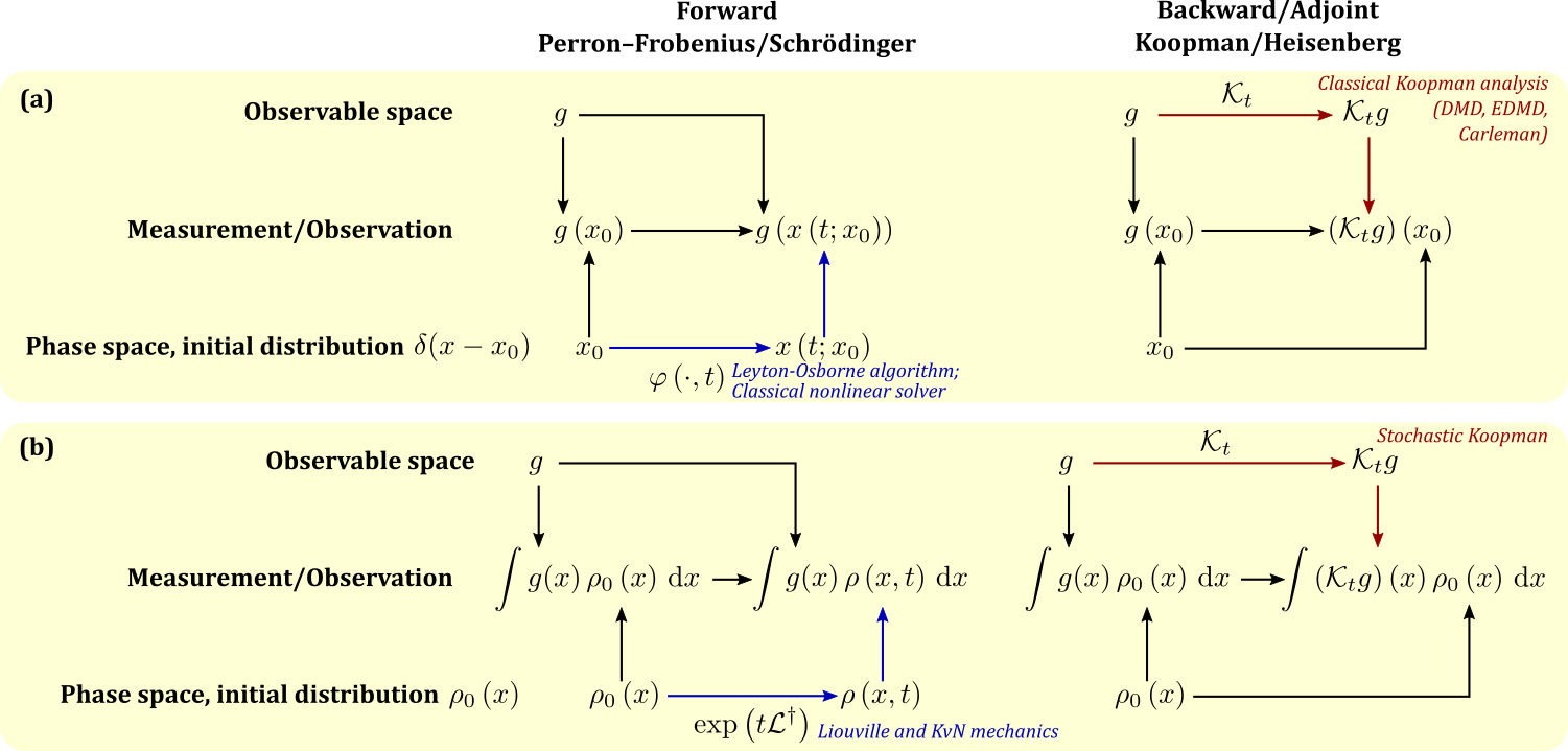
Figure 1: Schematic diagram of the relationship between the forward/Perron–Frobenius/Schrödinger representation and the backward/adjoint/Koopman/Heisenberg representation. In the forward picture, phase-space variables/distributions are evolving and the observables are fixed. In the backward picture, phase-space variables/distributions are fixed and the observables are evolving. (a) “Classical” systems given a single ($\delta$-distributed) initial condition; (b) “Classical statistical” systems given an initial distribution $\rho_{0}(x)$.

II.2 Perron–Frobenius representation

Both the Koopman representation and Koopman von Neumann mechanics are closely tied to the Liouville representation of dynamical systems. In contrast to setting a single initial condition of the phase-space representation described in Sec. (II.1), the Liouville representation introduces a probabilistic initial condition $x(0)$ that is distributed according to $\rho_{0}\equiv\rho(x,t=0)$, and derives a partial-differential equation describing how the distribution evolves by the flow $F$:

$$\frac{\partial}{\partial t}\rho(x,t)=-\sum_{j=1}^{N}\frac{\partial}{\partial x_{j}}\left[F_{j}\left(x\right)\rho\left(x,t\right)\right]=:\mathcal{L}^{\dagger}\rho(x,t).$$ (3)

Here, we define the forward operator $\mathcal{L}^{\dagger}$ which generates the evolution of the probability density. It is important to emphasize that the only probabilistic aspect of the system is its initial condition, given by the probability distribution, $\rho_{0}$. This initial distribution is propagated by the deterministic flow, $F$, to a later time, $\rho(x,t)$. Below, we denote the probability density at time $t$ as $\rho_{t}(x)\triangleq\rho(x,t)$. In the limit that $\rho_{0}$ approaches a Dirac $\delta$-distribution, the solution evolves as a $\delta$-distribution in the phase space $\mathbb{R}^{N}$ along the deterministic trajectory Eq. (2), and thus the Liouville representation is a generalization of the phase-space representation in Sec. II.1.

Note that the Liouville representation is linear in $\rho$: suppose $\rho^{(1)}$ and $\rho^{(2)}$ both satisfy Eq. (3), their linear combination $\alpha\rho^{(1)}+\beta\rho^{(t)}$, $\alpha$, $\beta\in\mathbb{R}$ also satisfies Eq. (3). The linearity and lack of the “sign problem” that plagues Quantum Monte Carlo Loh Jr et al. (1990); Van Bemmel et al. (1994); Troyer and Wiese (2005), leads to efficient Monte Carlo sampling for integrating (3): one first samples $N_{\text{MC}}$ initial conditions from $\rho_{0}$, then independently propagates the deterministic trajectories to $t\geq 0$ by Eq. (1) to obtain $N_{\text{MC}}$ samples of $\rho_{t}$.

We finally remark that when the dynamics are non-deterministic, the Liouville representation can be generalized to the so-called Perron–Frobenius representation Klus et al. (2018). For example, for the dynamical system Eq. (1), subject to isotropic Gaussian white noise, the Perron–Frobenius representation of the stochastic dynamical system is described by the Fokker–Planck Equation:

$$\frac{\partial}{\partial t}\rho(x,t)=-\nabla_{x}\cdot\left[F\left(x\right)\rho\left(x,t\right)\right]+\frac{D}{2}\nabla_{x}^{2}\left[\rho(x,t)\right],$$ (4)

where $D$ is the isotropic diffusion coefficient. In this case, we identify the forward generator $\mathcal{L}^{\dagger}=-\nabla_{x}F(x)+D\nabla^{2}_{x}/2$, where the differential operator $\nabla_{x}$ acts on everything to its right.

II.3 Koopman representation

In contrast to the Liouville and Perron–Frobenius representations, the other side of the coin is the Koopman representation Koopman (1931); Koopman and v. Neumann (1932); Mezić (2005). Instead of describing the evolution of the probability density in phase space, the Koopman representation aims to describe how “observables” evolve under the same dynamics. An observable is defined as a real- (or complex-) valued function, $g:\mathbb{R}^{N}\rightarrow\mathbb{R}$ (or $\mathbb{C}$), which maps the phase-space configuration $x$ to $g(x)$. In addition, an observable must be an $L^{2}\left(\mathbb{R}^{N},\text{d}\mu\right)$ function, meaning that it is square-integrable with respect to a specified measure $\text{d}\mu$:

$$\int_{\mathbb{R}^{N}}\left|g(x)\right|^{2}\text{d}\mu(x)<\infty.$$ (5)

In the Koopman representation, we will strictly consider the measure $\text{d}\mu$ to be a proper probability density with normalization, $\int_{\mathbb{R}^{N}}\text{d}\mu=1$. This technical condition ensures that for all observables of interest, $L^{2}\left(\mathbb{R}^{N},\text{d}\mu\right)$, also implies $L^{1}\left(\mathbb{R}^{N},\text{d}\mu\right)$, established by a simple application of Hölder’s inequality.

The central object in Koopman representation theory is a finite-time Koopman operator $\mathcal{K}_{t}$ which maps an $L^{2}\left(\mathbb{R}^{N},\rho_{t}(x)\,\text{d}x\right)$ function, $g$, to an $L^{2}\left(\mathbb{R}^{N},\rho_{0}(x)\,\text{d}x\right)$ function $\mathcal{K}_{t}g$, such that

$$\int_{\mathbb{R}^{N}}\left(\mathcal{K}_{t}g\right)\rho_{0}(x)\,\text{d}x=\int_{\mathbb{R}^{N}}g(x)\rho_{t}(x)\,\text{d}x.$$ (6)

That is, given an observable $g$, the expectation value of the observable against the evolving density $\rho_{t}$ is identical to the expectation value of $\mathcal{K}_{t}g$ against the initial density $\rho_{0}$. In the above equation, $\mathcal{K}_{t}g$ is integrable with respect to the initial distribution $\rho_{0}$, but $g$ is integrable against the later distribution, $\rho_{t}(\cdot)$, propagated by the dynamics. In the majority of applications, we are interested in ergodic processes after they converge to the invariant measure $\rho_{\text{inv}}$, which satisfies $\mathcal{L}^{\dagger}\rho_{\text{inv}}(x)=0$. In this case, we start the process at $\rho_{0}=\rho_{\text{inv}}$ and because of the stationarity, $\rho_{t}=\rho_{\text{inv}}$ for any $t\geq 0$. This leads to a simpler functional space, where we only care about those observables, $g$, and their evolution, $\mathcal{K}_{t}g$, that are in $L^{2}\left(\mathbb{R}^{N},\rho_{\text{inv}}\left(x\right)\text{d}x\right)$.

The $L^{2}$-integrability ensures a well-defined inner product operation between two $L^{2}\left(\mathbb{R}^{N},\text{d}\mu\right)$ functions $g_{1}$ and $g_{2}$:

$$\left\langle g_{1},g_{2}\right\rangle_{\mu}:=\int_{\mathbb{R}^{N}}g_{1}\left(x\right)\,g_{2}\left(x\right)\,\text{d}\mu.$$ (7)

As seen below, this inner product plays an important role in the Koopman representation. We will interchangeably use the Dirac bra-ket notation, $\left\langle g_{1}\large|g_{2}\right\rangle_{\mu}=\left\langle g_{1},g_{2}\right\rangle_{\mu}$.

A schematic diagram Fig. (1)(a) is commonly presented in the Koopman literature for a $\delta$-distributed initial condition; i.e., $x_{0}$ is a point in $\mathbb{R}^{N}$. Figure (1)(b) shows the slight generalization when we consider an initial distribution $\rho_{0}$ propagated by the nonlinear flow $F$. Importantly, the mapped observable $\mathcal{K}_{t}g$ depends on the initial condition $x_{0}$ in Fig. (1)(a), and is square-integrable with respect to the measure $\rho_{0}(x)\,\text{d}x$ in Fig. 1(b). Regardless of $t$, $\mathcal{K}_{t}$ always “pulls back” the function $g$, which is evaluated at the time $t\geq 0$ and integrable with respect to an evolving distribution $\rho_{t}$, to a function which is evaluated at the initial time $t=0$ with respect to a fixed distribution $\rho_{0}$.

The Koopman representation is linear even for those dynamical systems with nonlinear flow $F$ in the phase-space representation. The finite-time Koopman operator $\mathcal{K}_{t}$ is a linear operator, that is, given functions $g_{1},g_{2}\in L^{2}\left(\mathbb{R}^{N},\rho_{t}\left(x\right)\text{d}x\right)$ and arbitrary constants $\alpha,\beta\in\mathbb{R}$ or $\mathbb{C}$, $\mathcal{K}_{t}$ maps $\alpha g_{1}+\beta g_{2}$ to $\alpha\left(K_{t}g_{1}\right)+\beta\left(K_{t}g_{2}\right)$. Note that $\mathcal{K}_{t=0}$ is an identity mapping by definition. For any function $g\in L^{2}\left(\mathbb{R}^{N},\rho_{t}\left(x\right)\text{d}x\right)$, sending $t\downarrow 0$ implies that $g=\mathcal{K}_{0}g$ must be in $L^{2}\left(\mathbb{R}^{N},\rho_{0}\left(x\right)\text{d}x\right)$. Together with the inner product Eq. (7) with $\text{d}\mu\triangleq\rho_{0}(x)\text{d}x$, all $L^{2}\left(\mathbb{R}^{N},\rho_{0}\left(x\right)\text{d}x\right)$ functions form a Hilbert space. We remark that the inner product is uniquely defined as Eq. (7), against the initial probability density $\rho_{0}\left(x\right)$. Below, we denote the inner product by $\left\langle\cdot,\cdot\right\rangle_{\rho_{0}}$ for brevity.

In this Hilbert space, suppose we have a complete set of functional bases $\left\{f_{j}\right\}_{j}$ which linearly spans $L^{2}\left(\mathbb{R}^{N},\rho_{0}\left(x\right)\text{d}x\right)$, we can express any function $g=\sum_{j}\alpha_{j}f_{j}$ where $\alpha_{j}$’s are the coefficients. Because $\mathcal{K}_{t}f_{j}$ is another function in $L^{2}\left(\mathbb{R}^{N},\rho_{0}\left(x\right)\text{d}x\right)$, we can express $\mathcal{K}_{t}f_{j}$ as a linear sum of the basis functions, $\sum_{k}K_{j,k}(t)f_{k}$, where $K_{j,k}(t)$ are the linear coefficients characterizing the transformation. Immediately, we observe that $\mathcal{K}_{t}g=\sum_{j,k}\alpha_{j}K_{j,k}(t)f_{k}$—for any $g$, the finite-time Koopman operator linearly transforms the coefficients of the bases $\left\{f_{j}\right\}_{j}$, from $\left\{\alpha_{j}\right\}_{j}$ to $\left\{\sum_{k}\alpha_{k}K_{k,j}(t)\right\}_{j}$. The linearity of the Koopman representation enables the possibility of integration on a quantum computer, but comes with a trade-off: the operational space can be infinite dimensional: in most nonlinear systems, the number of indices ($i,j$) can be countably or (even worse) uncountably infinite. Even though the evolution of an observable $g$ depends linearly on other observables, this dependence can potentially involve infinitely many others; we observe similar problems in moment expansion methods Ale et al. (2013); Schnoerr et al. (2015) and Carleman linearizations Carleman (1932); Kowalski et al. (1991): the final closure is still an open problem, see the discussion in Lin et al. (2021). Nevertheless, in the classical (non-quantum) context, approximation methods take advantage of the linearity of the Koopman representation to transform the non-convex optimization problem of learning nonlinear systems into a globally convex problem, thus enabling data-driven modeling for complex and multiscale problems Schmid (2010); Williams et al. (2015a); Röblitz and Weber (2013).

The linear property of $\mathcal{K}_{t}$ motivates us to seek Koopman eigenvalue-eigenfunction pairs satisfying $\mathcal{K}_{t}\phi_{j}=e^{\lambda_{j}t}\phi_{j}$, $\lambda_{j}\in\mathbb{C}$ and $\phi_{j}\in L^{2}\left(\mathbb{R}^{N},\rho_{0}\left(x\right)\,\text{d}x\right)$ $\forall t\geq 0$. The Koopman eigenfunctions $\{\phi_{j}\}$ are thus the “good” functions whose evolution is invariant: one can write $\text{d}\left(\mathcal{K}_{t}\phi_{j}\right)/\text{d}t=\lambda_{j}\phi_{j}$. From Eq. (6), we also know that the time dependence of the expectation value of the observable $\sim e^{\lambda_{j}t}$. Furthermore, suppose we use these Koopman eigenfunctions as the basis functions to expand the functional space $L^{2}\left(\mathbb{R}^{N},\rho_{0}\left(x\right)\,\text{d}x\right)$, the linear decomposition of any function $g=\sum_{i}\beta_{j}\phi_{j}$ keeps its form under the evolution as $\mathcal{K}_{t}g=\sum_{j}\beta_{j}e^{\lambda_{j}t}\phi_{j}$. The Koopman eigenfunctions also characterize those invariant structures under the dynamics; for example, the leading Koopman eigenfunctions reveal basins of attraction in multistable systems Schmid (2010); Williams et al. (2015a).

Koopman showed that for Hamiltonian systems, the Koopman operators are always unitary, and thus, the Koopman eigenfunctions are mutually orthogonal, i.e, $\left\langle\phi_{j},\phi_{j}\right\rangle_{\rho_{0}}=\delta_{i,j}$. Nevertheless, because the Koopman operator of a general irreversible dynamical system is not guaranteed to be unitary, its Koopman eigenfunctions do not necessarily form an orthogonal basis set with the inner product (7). Nor are they required to be properly normalized. That is, $\left\langle\phi_{j},\phi_{j}\right\rangle_{\rho_{0}}\neq\delta_{i,j}$ in general, where $\delta_{i,j}$ is the Kronecker delta function. Consequently, the projection for solving the linear coefficients ($\alpha_{j}$ and $\beta_{j}$ above) often requires a proper normalization Alexandre J. Chorin et al. (2002); Williams et al. (2015a); Lin et al. (2021).

We finally remark that the $j$-notation ($\lambda_{j}$, $\phi_{j}$, $\sum_{j}$) is a stylized book-keeping notation. Since Koopman and von Neumann’s time, we have known that there are systems—for example, chaotic ones—with an uncountable number of eigenvalues Koopman and v. Neumann (1932); v. Neumann (1932); Mezić (2005, 2020). The spectrum of the Koopman operator of these systems has one or more continuous parts, and the functional space is an inseparable Hilbert space. In this case, we cannot express $j$ as a countable set, and the sum has to be separated into a sum over the point spectrum, and an integration over the continuous spectrum.

II.4 Forward v. backward, Schrödinger v. Heisenberg

The juxtaposition of Liouville (more generally, Perron–Frobenius) v. Koopman representations can be understood as the forward picture of a dynamical system v. the backward (adjoint) description of their observables. For simplicity, we first consider $\delta$-distributed initial conditions in this section. The solution of $g\left(x(t;x_{0})\right)$, that is, the $g$ function evaluated on the trajectory of the dynamical system with an initial condition $x_{0}$ can be obtained by solving the partial differential equation Alexandre J. Chorin et al. (2002):

$$\frac{\partial}{\partial t}\gamma(x,t)={} \mathcal{L}\gamma(x,t)\triangleq\sum_{j=1}^{N}F_{j}\frac{\partial}{\partial x_{j}}\gamma(x,t),$$

$$\gamma(x,0):={} g(x).$$ (8)

Note that the function $g$ is evaluated at $t=0$ as the initial data. The solution $\gamma(x,t)$ characterizes how the function $g$ “rides on” the dynamics: it is elementary to show that $\gamma(x_{0},t)=g(x(t;x_{0}))=\left(\mathcal{K}_{t}g\right)\left(x_{0}\right)$ is a spatiotemporal field of the $g$ function evaluated at the trajectory originated from $x_{0}$. The solution of $\gamma$ depends on $g$; by setting an identity function $g:=I$, i.e., $g(x)=x$, $\gamma$ is $\varphi$ in Eq. (2). Note that the above evolutionary equation (8) for $\gamma$ is also linear, again with the trade-off that one has to solve the infinite-dimensional field $\gamma:\mathbb{R}^{N}\times\mathbb{R}\rightarrow\mathbb{R}$.

The duality between the forward Liouville/Perron–Frobenius description and the backward (adjoint) Koopman description is most clear when we consider the expectation value of $g$ with respect to the probability density $\rho\left(x,t\right)$ Gerlich (1973):

$$\int_{\mathbb{R}^{N}}g(x)\,\rho(x,t)\,\text{d}x={} \int_{\mathbb{R}^{N}}\gamma(x,0)\,\rho(x,t)\,\text{d}x$$

$$={} \int_{\mathbb{R}^{N}}\gamma\left(x,t\right)\,\rho\left(x,0\right)\,\text{d}x$$ (9)

Here, the first line is the forward picture where the density is evolving, and the second line the Koopman picture where the observables are evolving. Moreover, the adjoint nature of these two pictures can be transparently observed if we use the Dirac bra-ket notation in the Hilbert space $L^{2}\left(\mathbb{R}^{N},\text{d}x\right)$:

$$\frac{\text{d}}{\text{d}t}\left\langle g,1\right\rangle_{\rho_{t}}={} \int_{\mathbb{R}^{N}}g(x)\,\mathcal{L}^{\dagger}\rho(x,t)\text{d}x$$ (10a)

$$={} \left\langle g,\mathcal{L}^{\dagger}\rho\left(t\right)\right\rangle=\left\langle\mathcal{L}\gamma\left(t\right)\large,\rho_{0}\right\rangle$$ (10b)

$$={} \int_{\mathbb{R}^{N}}\mathcal{L}\gamma\left(x,t\right)\rho_{0}\left(x\right)\text{d}x$$ (10c)

The operator $\mathcal{L}$ is exactly the adjoint of the Liouville operator, $\mathcal{L}^{\dagger}$, in Eq. (3). In terms of the Koopman representation, $\mathcal{L}$ is exactly the infinitesimal Koopman operator $\mathcal{K}:=\lim_{t\downarrow 0}\left(\mathcal{K}_{t}-1\right)/t$ Mauroy and Mezic (2016). In terms of stochastic processes, the adjoint operator is the Kolmogorov backward operator, which is the infinitesimal generator of a stochastic process.

Beside general dynamical system theory and stochastic processes, the best-known exhibition of such duality are the two pictures in the theory of quantum mechanics. The forward/Liouville/Perron–Frobenius representation is analogous to the Schrödinger picture, in which the quantum state evolves forward in time. The backward/adjoint/Koopman picture is analogous to the Heisenberg picture, in which the operators (observables) dynamically evolve forward in time.

II.5 Koopman von Neumann mechanics

Koopman von Neumann mechanics, hereinafter referred to as KvN mechanics, is a classical wave mechanics theory. Initially developed for Hamiltonian systems, this wave mechanics theory aims to bridge and unify the theories of classical and quantum mechanics. In most of the literature, Koopman and von Neumann were cited as the origin of KvN. However, we will see below that KvN is distinct from the backward/adjoint/Koopman representation in Koopman (1931); Koopman and v. Neumann (1932); v. Neumann (1932), and is in fact a forward Perron–Frobenius-Schrödinger representation.

Because classical Hamiltonian systems are the best and most intuitive way to understand KvN mechanics, we dedicate the next subsection only to Hamiltonian systems, with a following subsection generalizing the results to non-Hamiltonian systems.

II.5.1 Special case: Hamiltonian systems

The wavefunction is the fundamental description of a system’s state in quantum mechanics. With the motivation of bridging the classical and quantum mechanics, instead of the central object $\rho(x,t)$ in the Liouville representation, KvN mechanics focuses on a complex-valued classical wavefunction $\psi(x,t)$ with the Born rule $\rho(x,t)=\left|\psi(x,t)\right|^{2}:=\psi^{\ast}(x,t)\psi(x,t)$. Throughout this documentation, we reserve $\psi(x,t)$ to denote this classical KvN wavefunction and $\psi^{\ast}$ its complex conjugate.

Consider a Hamiltonian system, whose state consists of $N$ pairs of generalized coordinates $q_{j}$ and momenta $p_{j}$, $j=1\ldots N$. In previous notation $x=(q,p)$. A classical Hamiltonian ${H}(q,p):\mathbb{R}^{N}\times\mathbb{R}^{N}\rightarrow\mathbb{R}$ is defined and the system evolves according to Hamilton’s equation:

$$\dot{q}_{j}={} \frac{\partial{H}\left(q,p\right)}{\partial p_{j}},$$ (11a)

$$\dot{p}_{j}={} -\frac{\partial{H}\left(q,p\right)}{\partial q_{j}},$$ (11b)

$j=1\ldots N$. The Liouville equation (3) of the system is thus

$$\frac{\partial}{\partial t}\rho(q,p,t)={} \sum_{j=1}^{N}\frac{\partial}{\partial p_{j}}\left[\frac{\partial{H}\left(q,p\right)}{\partial q_{j}}\rho\left(q,p,t\right)\right]$$

$$-\sum_{j=1}^{N}\frac{\partial}{\partial q_{j}}\left[\frac{\partial{H}\left(q,p\right)}{\partial p_{j}}\rho\left(q,p,t\right)\right]$$

$$={} \sum_{j=1}^{N}\left(\frac{\partial{H}}{\partial q_{j}}\frac{\partial\rho}{\partial p_{j}}-\frac{\partial{H}}{\partial p_{j}}\frac{\partial\rho}{\partial q_{j}}\right).$$ (12)

In the last equation, we note that the special symplectic structure of the Hamiltonian led to the cancellation of the terms, $\partial^{2}H/\partial q_{j}\partial p_{j}-\partial^{2}H/\partial p_{j}\partial q_{j}=0$.

The fundamental object in KvN mechanics is the KvN wavefunction $\psi:\mathbb{R}^{N}\times\mathbb{R}^{N}\times\mathbb{R}\rightarrow\mathbb{C}$ which maps $(x,p,t)$ to a complex-valued “amplitude”. Immediately, one can show that the solution to a “classical” Schrödinger equation:

$$\frac{\partial\psi(q,p,t)}{\partial t}=\sum_{j=1}^{n}\frac{\partial{H}}{\partial q_{j}}\frac{\partial\psi}{\partial p_{j}}-\frac{\partial{H}}{\partial p_{j}}\frac{\partial\psi}{\partial q_{j}},$$ (13)

leads to the solution to the Liouville equation (12), with $\rho:=\psi^{\ast}\psi$. A more formal derivation of Eq. (13) from operator axioms can be found in Wilczek (2015). One defines the generator of the dynamics of the wavefunction:

$$\mathcal{L}^{\dagger}_{\text{KvN}}:=-\sum_{j=1}^{n}\dot{q}_{j}\frac{\partial}{\partial q_{j}}+\dot{p}_{j}\frac{\partial}{\partial p_{j}},$$ (14)

noting that it is identical to the generator of the dynamics of $\rho$, i.e., $\mathcal{L}$ in Eqs. (3) and (8). A KvN Hamiltonian is defined as

$$\mathcal{H}_{\text{KvN}}:=-i\mathcal{L}^{\dagger}_{\text{KvN}}=-i\sum_{j=1}^{n}\left(\dot{q}_{j}\frac{\partial}{\partial q_{j}}+\dot{p}_{j}\frac{\partial}{\partial p_{j}}\right)$$ (15)

where $\dot{q}$ and $\dot{p}$ are given by Eqs.(11a,11b) so that the evolutionary equation (13) for the KvN wavefunction resembles the Schrödinger equation:

$$i\frac{\partial}{\partial t}\psi(q,p,t)=\mathcal{H}_{\text{KvN}}\psi(q,p,t).$$ (16)

Note that neither $\hbar$ nor a phase is involved in this purely classical theory. The imaginary number $i$ is introduced, simply to make $H_{\text{KvN}}$ a Hermitian operator; see below. Equations (13) and (16) are completely equivalent, and KvN mechanics is fully classical. Contrary to quantum mechanics, the phase of the Koopman wavefunction is irrelevant, and thus the theory cannot be used to explain the double-slit experiment or Aharonov–Bohm effect.

Given any two test wavefunctions $\psi_{1}(x,t)=\psi_{1}(q,p,t)$ and $\psi_{2}(x,t)=\psi_{2}(q,p,t)$ in $L^{2}(\mathbb{R}^{2N},\text{d}x)$, using the Dirac bra-ket notation:

$$\left\langle\mathcal{H}_{\text{KvN}}^{\dagger}\psi_{1}(t)\right|\left.\vphantom{\mathcal{H}_{\text{KvN}}}\psi_{2}(t)\right\rangle=\left\langle\vphantom{\mathcal{H}_{\text{KvN}}}\psi_{1}(t)\right|\left.\mathcal{H}_{\text{KvN}}\psi_{2}(t)\right\rangle$$

$$={} \int_{\mathbb{R}^{2N}}\psi_{1}^{\ast}(x,t)\left[i\sum_{j=1}^{n}\frac{\partial H}{\partial q_{j}}\frac{\partial\psi_{2}(x,t)}{\partial p_{j}}-\frac{\partial H}{\partial p_{j}}\frac{\partial\psi_{2}(x,t)}{\partial q_{j}}\right]\text{d}x$$

$$={} \int_{\mathbb{R}^{2N}}\left[i\sum_{j=1}^{n}\frac{\partial H}{\partial q_{j}}\frac{\partial\psi_{1}(x,t)}{\partial p_{j}}-\frac{\partial H}{\partial p_{j}}\frac{\partial\psi_{1}(x,t)}{\partial q_{j}}\right]^{\ast}\psi_{2}(x,t)\text{d}x$$

$$={} \left\langle\mathcal{H}_{\text{KvN}}\psi_{1}(t)\right|\left.\vphantom{\mathcal{H}_{\text{KvN}}^{\dagger}}\psi_{2}(t)\right\rangle,$$ (17)

we thus conclude that $\mathcal{H}_{\text{KvN}}=\mathcal{H}_{\text{KvN}}^{\dagger}$, i.e., it is a Hermitian operator. Note that the negative sign of the complex conjugate of $i$ is cancelled by the negative sign from the integration by parts. We also assume the boundary terms are zero, imposed by the typical requirement of wavefunctions $\left|\psi\right|\rightarrow 0$ at the boundaries. The Hermitian property results in the unitary propagator $\exp\left(-it\mathcal{H}_{\text{KvN}}\right)$, and the normalization $\int_{\mathbb{R}^{2N}}\psi^{\ast}(x,t)\,\psi(x,t)\,\text{d}x$ is preserved under the dynamics. Note that a Hermitian $\mathcal{H}_{\text{KvN}}$ implies an anti-self-adjoint $\mathcal{L}^{\dagger}_{\text{KvN}}\equiv-i\mathcal{H}_{\text{KvN}}$.

We emphasize that the expression resembles the formulation in quantum mechanics only at a superficial level: the resulting propagator is exactly the classical propagator $\exp\left(t\mathcal{L}_{\text{KvN}}\right)$, once we plug in $\mathcal{H}_{\text{KvN}}:=i\mathcal{L}^{\dagger}_{\text{KvN}}$. The normalization is conserved because the Liouville operator $\mathcal{L}^{\dagger}_{\text{KvN}}$ only moves the probability mass in the phase space from one configuration to another. Note also that the generator $\mathcal{H}_{\text{KvN}}$ is not the operator form of the Hamiltonian in quantum mechanics which substitutes the momentum $p$ by $\left({\hbar}/{i}\right)\partial_{q}$: In the classical KvN mechanics, the momentum and position are commuting ($[{q}_{j},{p}_{j}]=0$), in contrast to the canonical commutation relation between the position and momentum operators in quantum mechanics, $[\hat{q}_{j},\hat{p}_{j}]=i\hbar\hat{I}$ (we use $\hat{\cdot}$ to denote quantum-mechanical operators).

II.5.2 General nonlinear dynamical systems

With the same spirit, for a general dynamical system following (3), it is possible to prescribe a classical Schrödinger equation Yu. I. Bogdanov and N. A. Bogdanova (2014); Yu. I. Bogdanov et al. (2019); Joseph (2020):

$$\frac{\partial\psi(x,t)}{\partial t}=-\sum_{j=1}^{n}\left[F_{j}(x)\frac{\partial}{\partial x_{j}}+\frac{1}{2}\frac{\partial F_{j}(x)}{\partial x_{j}}\right]\psi\left(x,t\right),$$ (18)

such that $\rho(x,t)\equiv\psi^{\ast}(x,t)\psi(x,t)$ solves (3). Note that the state space is $\mathbb{R}^{N}$, so the KvN wavefunction $\psi:\mathbb{R}^{N}\times\mathbb{R}\rightarrow\mathbb{C}$ (in contrast to the $2N$-dimensional Hamiltonian systems). Because the KvN Hamiltonian, defined as

$$\mathcal{H}_{\text{KvN}}:=-i\sum_{j=1}^{n}\left[F_{j}(x)\frac{\partial}{\partial x_{j}}+\frac{1}{2}\frac{\partial F_{j}(x)}{\partial x_{j}}\right],$$ (19)

is Hermitian, the propagator is again unitary and the normalization is preserved under the dynamics. It is tempting to define $\partial_{x_{j}}$ in (13) or (18) as auxiliary operators $\mathcal{P}_{j}:=-i\partial_{x_{j}}$ Yu. I. Bogdanov and N. A. Bogdanova (2014); Yu. I. Bogdanov et al. (2019); Joseph (2020) and symmetrize the operator into the form

$$\mathcal{H}_{\text{KvN}}=\frac{1}{2}\sum_{j=1}^{n}\left(\mathcal{P}_{j}F_{j}(x)+F_{j}(x)\mathcal{P}_{j}\right).$$ (20)

Here, the $\mathcal{P}_{j}$ operates on everything to its right, i.e., for two test functions $f$ and $g$, $\mathcal{P}_{j}\left(fg\right):=\left(\mathcal{P}_{j}f\right)g+f\left(\mathcal{P}_{j}g\right)$. Note that this auxiliary operator is not the momentum of a Hamiltonian system, that is, $p_{j}$ in (13): the position $x_{j}$ commutes with $p_{j}$ in KvN mechanics, but not with $\mathcal{P}_{j}$. It is most clear in the axiomatic construction of the KvN mechanics in Wilczek (2015), in which $\partial_{x_{j}}$ is denoted by an operator $\lambda_{x_{j}}$ and is not associated with the classical momenta. Identifying $\partial_{x_{j}}$ as a momentum, such as in Joseph (2020), should not be considered as a fully classical KvN mechanics. Such an indentification would invoke the quantum mechanical Stone-von Neumann theorem, which specifies the momentum operator $\mathcal{P}_{j}=-i\partial_{x_{j}}$ (in the unit $\hbar=1$) in the position representation and results in the Heisenberg uncertainty principle. In terms of KvN mechanics, $\mathcal{P}_{j}$ should be considered as merely an operator in the Hilbert space.

For completeness, we present a further, alternative construction of KvN mechanics that we have not seen in the quantum literature, that uses the fact that one can construct a Hamiltonian system in an augmented space $\mathbb{R}^{2N}$ for any non-Hamiltonian system (1). To achieve this, we take a path-integral approach and begin with an action for a trajectory $x(t)$, $0\leq t\leq T$:

$$A\left[x\right]={} \int_{0}^{T}L\left(\dot{x}(t),x(t)\right)\,\text{d}t$$

$$\triangleq{} \int_{0}^{T}\sum_{j=1}^{N}\left[\dot{x}_{j}(t)-F_{j}(x(t))\right]^{2}\,\text{d}t.$$ (21)

The Lagrangian $L$ is proportional to the Onsager–Machlup function; the action can be considered as the scaled Onsager–Machlup functional for diffusion processes with white noise in the zero-noise limit Yasue (1979). Note that the action is minimized when $\dot{x}(t)$ follows the evolutionary equation (1). The conjugate momentum of the Lagrangian, $\varpi_{j}$, can be solved by $\varpi_{j}=\partial L/\dot{x}_{j}=\dot{x}_{j}-F_{j}(x)$. The augmented Hamiltonian can then be constructed via a Legendre transform

$$H_{\text{aug}}(x,\varpi):={} \sum_{j=1}^{N}\varpi_{j}\dot{x}_{j}-L=\sum_{j=1}^{N}\varpi_{j}\left(\varpi_{j}+F_{j}\right)-\varpi_{j}^{2}$$

$$={} \sum_{j=1}^{N}\varpi_{j}F_{j}=\frac{1}{2}\sum_{j=1}^{N}\left(\varpi_{j}F_{j}+F_{j}\varpi_{j}\right).$$ (22)

Despite the resemblance to the form of Eq. (20), it is important to realize that they are not the same: $\mathcal{P}_{j}:=-i\partial_{x_{j}}$ and $x$ are non-commuting, but the classical $\varpi_{j}$ and $x_{j}$ are commuting. Hamilton’s equation prescribes the evolution of $x$ and $\varpi$:

$$\dot{x}_{j}={} \partial_{\varpi_{j}}\mathcal{H}_{\text{aug}}=F_{j}\left(x\right),$$ (23a)

$$\dot{\varpi}_{j}={} -\partial_{x_{j}}\mathcal{H}_{\text{aug}}=-\sum_{k=1}^{N}\varpi_{k}\frac{\partial F_{k}\left(x\right)}{\partial x_{j}}.$$ (23b)

Note that the solution of $x$ is consistent with that of (1). However, following the KvN construction on this classical Hamiltonian system leads to a distinct generator from Eq. (20):

$$\mathcal{H}_{\text{KvN}}^{(2N)}=-\frac{i}{2}\sum_{j=1}^{N}\left[F_{j}\left(x\right)\frac{\partial}{\partial x_{j}}-\sum_{j=k}^{N}\varpi_{k}\frac{\partial F_{k}\left(x\right)}{\partial x_{j}}\frac{\partial}{\partial\varpi_{j}}\right],$$ (24)

with the Schrödinger equation

$$i\frac{\partial}{\partial t}\psi\left(x,\varpi,t\right)=\mathcal{H}_{\text{KvN}}^{(2N)}\psi\left(x,\varpi,t\right)$$ (25)

Note that the KvN wavefunction $\psi(x,\varpi,t)$ in this construct lives in a higher-dimensional space, $\mathbb{R}^{2N}$; we thus decorate the Hamiltonian by a superscript $(2N)$. The auxiliary operators are now $-i\partial_{x_{j}}$ and $-i\partial_{\varpi_{j}}$, and the classical conjugate momentum is $\varpi$.

In the discussion below, we will strictly focus on $\mathcal{H}_{\text{KvN}}$ which lives in a smaller dimension and leave the existence of $\mathcal{H}_{\text{KvN}}^{(2N)}$ as an intriguing observation.

II.5.3 Spectral analysis of the KvN Hamiltonian

It is natural to solve the linear KvN Schrödinger equation by identifying the eigenvalue $\nu_{j}$ and eigenvector $\chi_{j}$ pairs satisfying

$$\mathcal{H}_{\text{KvN}}\chi_{j}=\nu_{j}\chi_{j}.$$ (26)

Because $\mathcal{H}_{\text{KvN}}$ is Hermitian, the eigenvalues $\nu_{j}$’s are real and the eigenvectors are mutually orthogonal $\left\langle\chi_{j},\chi_{j}\right\rangle=\delta_{i,j}$. Again, the Hilbert space here is $L^{2}\left(\mathbb{R}^{N},\text{d}x\right)$. The full solution can then be expressed as

$$\psi(x,t)=\sum_{i}\kappa_{j}e^{-i\nu_{j}t}\chi_{j}(x),$$ (27)

where $\kappa_{j}$’s are the complex-valued coefficients satisfying the initial condition, $\kappa_{j}=\left\langle\chi_{j},\psi(t=0)\right\rangle$.

If (1) is linear, then the spectrum of $x$ is related to the spectrum of $\rho(x,t)$ ROWLEY et al. (2009). For KvN, the relationship between spectra is not clear; note that the transformation from $\rho(x,t)$ to $\psi(x,t)$ is nonlinear (quadratic). More discussion of the spectral differences is given in the next section.

II.6 Differences between the Koopman representation and Koopman von Neumann mechanics

We are now in a position to list some of the major differences between the Koopman representation and KvN mechanics. Our central result is that Koopman von Neumann mechanics is not a Koopman representation. The most fundamental observation which sets the tone of this statement is: The Koopman representation is the Heisenberg/adjoint/backward picture, and Koopman von Neumann mechanics is the Schrödinger/forward picture. Despite their being two sides of the same coin, the two interpretations create ramifications below.

Different objects evolving in time. In the Koopman representation, we aim to describe the evolution of observables, which are integrable functions of an initial condition with respect to an initial distribution; in Koopman von Neumann mechanics, we aim to describe the evolution of a KvN wavefunction, which is related to a probability distribution. Note that the symbols $\psi$ (and $\varphi$) in the original Koopman paper Koopman (1931) are functions of the initial microscopic state, and not a wavefunction, which is a function of state space and time.

Different inner-product spaces. The Koopman representation lives in the Hilbert space $L^{2}\left(\mathbb{R}^{N},\rho_{0}\left(x\right)\text{d}x\right)$, equipped with the inner product $\left\langle\cdot,\cdot\right\rangle_{\rho_{0}}$, that is, Eq. (7) with $\text{d}\mu=\rho_{0}\left(x\right)\text{d}x$. For ergodic systems, it is common to initiate the system at the invariant measure and define the inner product by the invariant measure $\text{d}\mu=\rho_{\text{inv}}\left(x\right)\text{d}x$. Note that in Koopman (1931), the probability density $\rho$ is always there in the inner product. In contrast, the KvN mechanics lives in the Hilbert space $L^{2}\left(\mathbb{R}^{N},\text{d}x\right)$ equipped with the inner product $\left\langle\cdot,\cdot\right\rangle$ between two KvN wavefunctions, that is, Eq. (7) with the Lebesgue measure $\text{d}\mu=\text{d}x$.

Different generators and propagators. Koopman Koopman (1931) showed that for Hamiltonian systems, the propagator for the observables, the finite-time Koopman operator $\mathcal{K}_{t}$ is unitary (and thus Koopman denoted it by $U_{t}$), and deduced via the Stone’s theorem on one-parameter unitary groups that the infinitesimal Koopman operator $\mathcal{K}:=\lim_{t\downarrow 0}\left(\mathcal{K}_{t}-1\right)/t$ is anti-self-adjoint (in the original paper, $\mathcal{K}=iP$ is anti-self-adjoint because $P$ is self-adjoint/Hermitian). For general irreversible systems, it is known that the Koopman operator does not have to be unitary (see examples in Williams et al. (2015a)). As for KvN mechanics, the generator of the KvN wavefunction dynamics (i.e., $-i\mathcal{H}_{\text{KvN}}$) is always anti-self-adjoint, regardless of whether $F$ is a Hamiltonian flow. In the case of a Hamiltonian system, the divergence term $\sum_{j=1}^{N}\partial_{x_{j}}F_{j}=0$ because the flow of the full state $x=(q,p)$ is volume conserving, and Eq. (19) is identical to Eq. (15).

Different spectra and basis functions. For a general irreversible system, the Koopman operator $\mathcal{K}_{t}$ does not have to be unitary, so $|e^{\tau\lambda_{j}}|$ are not necessarily $1$ for any $\tau\geq 0$. That is, observables do not conserve their norm under the dynamics. Koopman eigenfunctions $\phi_{j}$’s are not necessarily orthogonal to each other. Note that the Koopman spectrum is shared with its adjoint, the Perron–Frobenius transfer operator and the forward infinitesimal operator $\mathcal{L}^{\dagger}$ Klus et al. (2018). In terms of KvN mechanics, by construction $\mathcal{H}_{\text{KvN}}$ is Hermitian, which guarantees $|e^{i\tau\nu_{j}}|=1$ for any $\tau\geq 0$ and orthogonal $\chi_{j}$’s. That is, observables conserve their norm under the dynamics. The KvN decomposition is closely related to the Proper Orthogonal Decomposition (POD) Lumley (2007); Sirovich (1987); Berkooz et al. (1993). As concisely summarized in Schmid’s original paper Schmid (2010) on Dynamic Mode Decomposition, which is a Koopman representation but restricted only to linear observables, the Koopman representation attempts to capture the orthogonality “in time”, and the POD (and the KvN mechanics here) attempts to capture the orthogonality “in space”.

KvN mechanics is a wave mechanics with perpetually oscillating eigenfunctions, which may not be true for Koopman eigenfunctions. A natural and interesting consequence of the differences of the spectra of these two formulations is that, the solution in KvN mechanics is purely composed of oscillatory eigenfunctions, while the Koopman eigenfunctions can be both decaying and oscillatory. Let us consider a simple, one-dimensional decaying dynamics, $\dot{x}=-x^{2}$ on a strictly positive domain $x\in\mathbb{R}^{+}$, which was presented as an illustrative example in Lin et al. (2021). We can show that a Koopman eigenfunction of this problem is $g(x)=\exp\left(-1/x\right)$ and $\mathcal{K}g=-g$, and $\lambda=-1$ clearly indicating the dissipating nature of the dynamics. On the other hand, the KvN wavefunctions are always oscillatory. Similar to using Fourier modes to describe exponentially decaying signals, in the $\dot{x}=-x^{2}$ example, to describe the dynamics of a single Koopman eigenfunction $g(x)=\exp\left(-1/x\right)$ requires infinitely many KvN eigenfunctions.

Relationship between two operators $\mathcal{H}_{\text{KvN}}$ and $\mathcal{K}$. We can use the evolutionary equation of the expectation value of an observable $g:\mathbb{R}^{N}\rightarrow\mathbb{R}$ with respect to the probability density $\psi^{\ast}(x,t)\psi(x,t)$ to establish the formal relationship between the infinitesimal Koopman operator $\mathcal{K}$ and the KvN Hamiltonian $\mathcal{H}_{\text{KvN}}$ (below, integrals are over the entire space $\mathbb{R}^{N}$):

$$\frac{\text{d}}{\text{d}t}\left\langle g\right\rangle(t)=\frac{\text{d}}{\text{d}t}\int\psi^{\ast}\left(x,t\right)g\left(x\right)\,\psi\left(x,t\right)\text{d}x.$$ (28)

Using the KvN Schrödinger equation,

$$\frac{\text{d}}{\text{d}t}\left\langle g\right\rangle(t)={} \int\left(-i\mathcal{H}_{\text{KvN}}\psi\right)^{\ast}g\,\psi\,\text{d}x$$

$$+\int\psi^{\ast}\,g\left(-i\mathcal{H}_{\text{KvN}}\psi\right)\text{d}x.$$ (29)

We next use the self-adjointness of the operator $\mathcal{H}_{\text{KvN}}$ to transfer the $\mathcal{H}_{\text{KvN}}$ in the first term to the observable $g$:

$$\frac{\text{d}}{\text{d}t}\left\langle g\right\rangle{} (t)=i\int\psi\left(\mathcal{H}_{\text{KvN}}g-g\mathcal{H}_{\text{KvN}}\right)\psi\,\text{d}x.$$ (30)

We now switch to the adjoint/backward/Heisenberg picture to make the connection to the Koopman representation. The observable is now time-dependent, i.e., $\gamma(x,t)$ in Eq. (8), such that

$$\frac{\partial}{\partial t}\gamma\left(x,t\right)=i\left[\mathcal{H}_{\text{KvN}}\gamma\left(x,t\right)-\gamma\left(x,t\right)\mathcal{H}_{\text{KvN}}\right].$$ (31)

Next, plugging in the definition of $\mathcal{H}_{\text{KvN}}$, Eq. (19), on a test function $\psi$:

$$\mathcal{H}_{\text{KvN}}\gamma\psi={} -i\left[\sum_{j=1}^{N}F_{j}\frac{\partial\gamma}{\partial x_{j}}\psi+F_{j}\gamma\frac{\partial\psi}{\partial x}+\frac{1}{2}\frac{\partial F_{j}}{\partial x_{j}}\right],$$

$$\gamma\mathcal{H}_{\text{KvN}}\psi={} -i\gamma\left[\sum_{j=1}^{N}F_{j}\frac{\partial\psi}{\partial x}+\frac{1}{2}\frac{\partial F_{j}}{\partial x_{j}}\right],$$ (32)

noting that $F_{j}(x)\gamma(x,t)=\gamma(x,t)F_{j}(x)$, we arrive at the operator equation

$$\frac{\partial}{\partial t}\gamma\left(x,t\right)={} \sum_{j=1}^{N}F_{j}(x)\frac{\partial\gamma(x,t)}{\partial x_{j}}$$

$$={} \left[\mathcal{L}\gamma\right]\left(x,t\right)=\left[\mathcal{K}\gamma\right]\left(x,t\right).$$ (33)

Finally, we identify the relationship between the infinitesimal Koopman operator and the KvN Hamiltonian: given any test observable $\gamma=\gamma\left(x,t\right)$,

$$\mathcal{K}\gamma=i\left[\mathcal{H}_{\text{KvN}}\gamma-\gamma\mathcal{H}_{\text{KvN}}\right].$$ (34)

The fact that the right hand side of the equation resembles the Heisenberg equation should not be a surprise: the infinitesimal Koopman operator is the generator of the operator dynamics.

III Quantum computation for solving dynamical systems

There are (at least) two difficulties when solving nonlinear equations using a classical computer: (i) The original system of interest is very high dimensional, such that classical computers run into memory issues, but perhaps the system can be encoded in the exponentially sized Hilbert space of a quantum computer. (ii) The system of interst is not necessarily high dimensional but is highly nonlinear (maybe chaotic), such that classical computers run into precision issues.

We have already established that finite dimensional nonlinear systems can be mapped to infinite dimensional linear systems which can then be approximated in a reduced computational space by finite dimensional linear systems using the methods outlined in the previous section. Since the nonlinearity is absent in this approach, it might appear that precision is not a problem and we don’t need to worry about (ii). This is not the case, however, because the linear dynamics of the reduced system might not represent the nonlinear dynamics faithfully. On the other hand, one might hope that this issue can be alleviated by using very large dimensional linear systems. Quantum computation does have the advantage that the dimension of the operational space scales exponentially with the number of underlying computational units (e.g., qubits); thus, the hope is that a sufficiently large space could allow us to overcome both difficulities (i) and (ii).

One tempting classical way to numerically solve an initial-value problem for a complex nonlinear dynamical system is to integrate the evolutionary equation (1) forward in time in the phase-space picture. Consider explicit Euler time-integration, with a uniform time step $\Delta$. The numerical process entails: (1) start from the initial state, $x_{0}$, (2) evaluate the RHS of Eq. (1) at time $0$, (3) compute the state at time $\Delta$ by $x_{\Delta}:=x_{0}+F\left(x_{0}\right)\Delta$, (4) iterate steps (2-3) until the terminal time $T$.

Importantly, for nonlinear systems, step (2) requires a nonlinear operation on $x$ to compute the flow at subsequent times, $F(x_{m\Delta})$. For this scheme, we cannot bypass the nonlinear operation.

When we implement this procedure on a quantum computer an exponential number of initial states (in the number of time steps) are required to integrate the equation Leyton and Osborne (2008). This can be seen in the simple case of a quadratic nonlinearity, where the variable $x$ is encoded in a quantum state $|\psi_{t}\rangle=\sum_{i}\psi_{t,i}|i\rangle$ via $x_{i}(t)\propto\psi_{t,i}$. Due to linearity, two copies of the state $|\psi_{t}\rangle$ at time $t=m\Delta$ are needed to prepare a quantum state with amplitudes proportional to $x_{i}(t)^{2}$. Moreover, the algorithm that achieves this consumes the two copies in the process Leyton and Osborne (2008). On the other hand, copies can not be created on demand due to the no-cloning theorem: they have to be prepared individually using the same procedure instead. Thus, we see that, for an integration time $T=N\Delta$, of order $2^{N}$ copies of $|\psi_{0}\rangle$ will be needed to integrate the equation. As such, this approach is not computationally feasible on a quantum computer.

Instead, the linearity of the representations presented in the previous section opens a door for using quantum computation (QC) for solving nonlinear dynamical systems. If the resulting linear differential equations, expressed as $\dot{\mathbf{x}}(t)=\mathbf{L}\cdot\mathbf{x}(t)$, satisfy some technical requirements (see Berry (2014) for details), we can leverage quantum algorithms for (1) simulating the finite-time propagator $e^{t\mathbf{L}}$ if $i\mathbf{L}$ is Hermitian Berry et al. (2007) and (2) an algorithm proposed by Berry for solving general linear differential equations Berry (2014), if $i\mathbf{L}$ does not have the desired Hamiltonian structure. KvN mechanics produces a set of equations that can be solved with both (1) and (2), but the Koopman representation will in general require the more general approach (2) unless the Koopman operator, itself, is Hermitian.

Potential pitfalls and technical difficulties exist even with perfect QC implementations for solving linear dynamical systems. This is mainly due to a trade-off between linearity and the dimension of the representation. In order to gain linearity in these representations, the dimensionality of the operational space is generally infinite. In practice, it is necessary to perform some form of truncation, projection, or discretization, which reduces the computational space to finite-dimensionality but inevitably induces errors.

We will use the toy example $x(t)=-x^{2}(t)$ in each of the representations. We provide parallel analyses on an alternative model, the two-dimensional Van der Pol oscillator, in Appendix B, showing our observations below are generic and not dependent on the specific toy example we chose. We believe that the conclusions we draw from the examples will be applicable to high dimensional systems as well.

III.1 The Koopman representation

The central idea of using the Koopman representation in QC is its linear evolution in the observable space. As such, given a complete set of observables, evaluated at the initial condition, the IVP is a linear problem which can, in principle, be solved with a quantum linear systems algorithm. However, there are two major challenges. First, observables can contain nonlinear functions of the initial condition, thus to enable end-to-end QC, one needs a general circuit for arbitrary nonlinear transformation of the initial condition $x$ to $g(x)$. This is a challenging problem, and will, necessarily, require multiple copies of an initial state, however, it does not necessarily lead to the same exponential blow-up in resources as the Leyton-Osborne approach Leyton and Osborne (2008), as the generation of the nonlinear initial state (and possibly the inverse transformation at the end of the computation) only need be performed once. Second, it is not necessarily true that the quantity of interest can be embedded in a finite set of observables, i.e., the minimal Koopman invariant space is not guaranteed to be finite dimensional.

Even with the existence of a finite set, the set is not known a priori and the number of observables spanning the invariant space may be very large. In any case, a certain approximation by a smaller set of observables is needed, which induces the closure problem. Although such a problem can be solved by data-driven projection when simulation data are available, in our case, the purpose of solving the IVP is to generate simulation data. As such, the projection operator of the closure scheme must be sought via other system-specific means. Furthermore, the approximation often has a short accurate predictive horizon. Higher-order methods such as time-embedded DMD or Mori–Zwanzig formalism Lin et al. (2021) exist, but they do not fully resolve the closure problem.

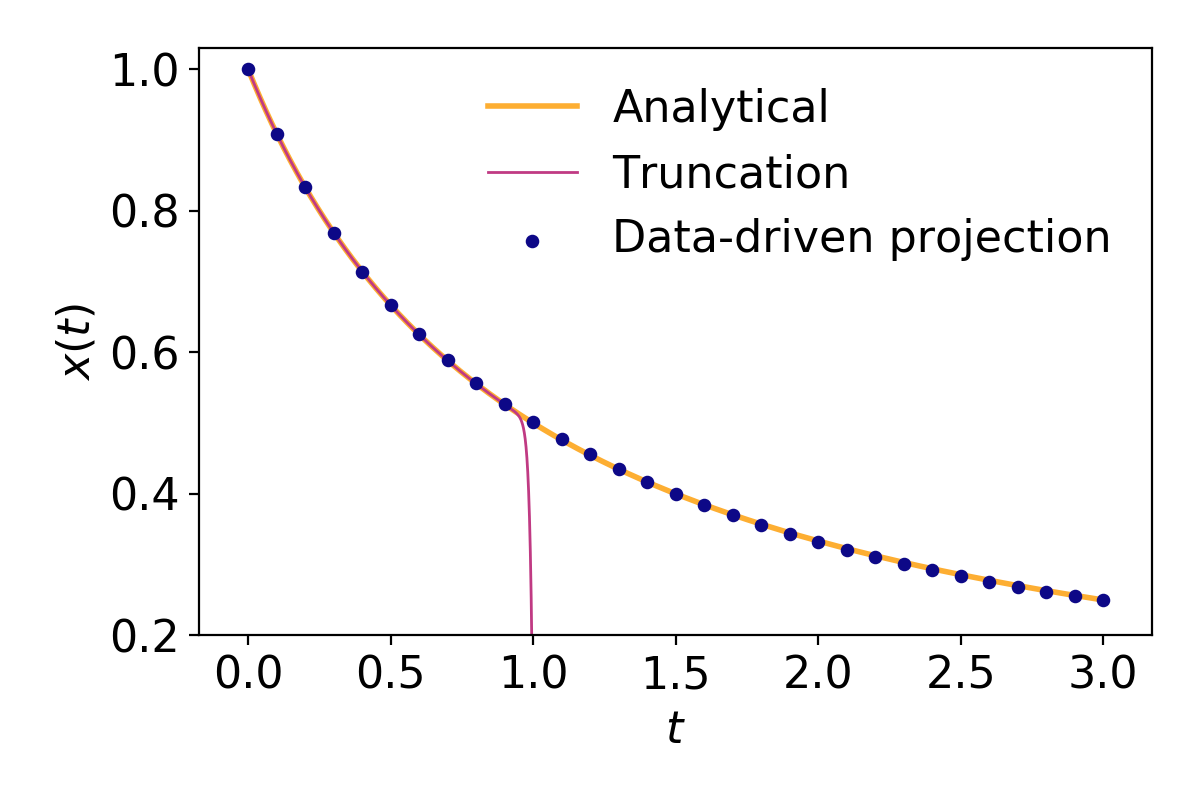
Figure 2: Carleman linearization with truncation at the first hundred order and approximate Koopman projection to a subfunctional space spanned by only the first three order.

Example. Consider $\dot{x}=-x^{2}$, and suppose we choose the polynomial observables, $g_{n}(x):=x^{n}$, $n=0,1,\ldots.$ This is the Carleman linearization. The linear equation of the observables is $\dot{g}_{n}=-ng_{n+1}$, $n=1,\ldots$ When solving this problem with a QC, we encode the vector $g=(g_{0},g_{1},\dots)$ as a quantum state $|\psi(t)\rangle\propto\sum_{n}g_{n}\left(x(t)\right)|n\rangle$. The goal of the algorithm is to output this state, which can then be used to compute properties of the solution, which is encoded in one of the amplitudes, $g_{1}\left(x(t)\right)$. 

Because $\dot{g}_{n}$ always depends on $g_{n+1}$, a proper closure scheme is needed. To showcase potential problems that can arise in closure schemes, we consider (1) truncating at $100^{\text{th}}$ order, i.e., $\dot{g}_{100}=0$ or equivalently $g_{101}=0$ and (2) projecting the infinite-dimensional series onto the first three polynomial functions, that is, assuming $\left[{\bf g}\left(x\left(t+\delta\right)\right)\right]\approx\mathbf{K}_{\delta}\cdot\left[{\bf g}\left(x\left(t\right)\right)\right]$ where $\left[g\right]$ is the stacked column vector of $g_{0}$, $g_{1}$, and $g_{2}$ and $\mathbf{K}_{\delta}$ is the approximate finite-time ($\delta$) Koopman operator. We remark that other closure schemes are possible; we do not aim to present an exhaustive analysis on closure schemes here, but we aim to use our examples to illustrate potential problems. We also note here that, many sophisticated moment closure schemes require nonlinear operations, e.g., $g_{101}\approx g_{50}g_{51}$. As explained above, it is not desirable to deploy nonlinear operations for integrating/evolving the system forward in time. Closure schemes using linear superpositions of the observables in the set to approximate the $g_{101}$, which is the essence of our second scheme leveraging projection via the EDMD procedure Williams et al. (2015a) when data is available, outlined below.

Assuming perfect snapshots of $\left[{\bf g}\left(x\left(t\right)\right)\right]$ are available at $t=0,\delta,2\delta,\ldots$ for us to minimize the $L^{2}$ norm between the true solution and this projected dynamics in this 3-dimensional projected space, we use the minimizer $K_{\delta}$ for integrating the linear system forward for making prediction. Here, we choose $\delta=0.1$, and use the analytical solution to numerically solve for the minimizer $K_{\delta}$:

$$\mathbf{K}_{\delta=0.1}=\begin{bmatrix}1.&-0.&0.\\ 0.001&0.992&-0.084\\ -0.025&0.156&0.699\\ \end{bmatrix}.$$ (35)

The aim of this analysis is to show the quality of prediction of a three-dimensional linear approximation of the infinite-dimensional Koopman representation, if we can obtain the approximate propagator $\mathbf{K}_{0.1}$ by means other than QC.

Both closure schemes lead to the standard linear problem of the form $\dot{\mathbf{x}}=\mathbf{L}\cdot\mathbf{x}$. Here, the elements of $\mathbf{x}$ are the $g_{i}$’s; $\mathbf{L}$ is a sparse, superdiagonal matrix in the first closure scheme, and simply $\mathbf{K}_{\delta}$ with the second closure scheme. In both cases, we can use Berry’s algorithm or improvements thereof Berry (2014); Berry et al. (2017) to solve the linear problem. To showcase the potential problem arising from the closure schemes, we use the high-accuracy general-purposed integration scipy.optimize.solve_ivp with lsoda to mimic a fault-tolerant QC implementation of the Berry’s algorithm, in the limit of extremely small time steps. We stress that all of our numerical results in this study were generated on a classical computer, in order study the properties of the numerical solution in an idealized setting. We assume $x(0)=1.0$ and evolve the system to $t=3$. The result can be seen in Fig. 2, that this typical truncation scheme would be problematic for a long prediction horizon even with a very high order closure. However, the projection approach is more controllable even with a small (only three) set of observables considered. The apparent chicken-and-egg problem of using a QC and an approximate Koopman operator is that the approximate Koopman operator $\mathbf{K}_{\delta}$ of a complex dynamical system is generally not analytically tractable, so we need to rely on a data-driven approach to retrieve it numerically from the simulated trajectories. If we can already simulate the trajectories of a complex dynamical system, it is unclear what the advantage of a QC would be.

Note that the results in Fig. 2 are consistent with the error bound derived in Ref. (Forets and Pouly, 2017, Eq. (27)), which for this problem, reduces to

$$\|\varepsilon(t)\|\leq\frac{t^{n}}{1-t}\,,$$ (36)

which clearly is unbounded as $t\rightarrow 1$.

Finally, as pointed out in Lin et al. (2021), the system has a one-dimensional Koopman invariant space $g_{\ast}(x)=\exp(-1/x)$, which follows $\dot{g}_{\ast}=-g_{\ast}$. Suppose we know such an invariant space (not necessarily one dimensional) and wish to leverage it to perform a classical simulation on a QC, we would need the nonlinear transformation $g_{\ast}$ to initiate the observable, linearly integrating it forward in time by QC, and then applying the nonlinear inverse transformation $g^{-1}_{\ast}(x)=-1.0/\log(x)$ to obtain $x$.

It is currently challenging to implement both of these nonlinear transformations on a QC. Such an invariant space idea is tightly connected to the idea of constant of integration methods of integrable systems. For example, it is known that for a nonlinear Burgers’ equation, we can perform the Cole–Hopf transformation (c.f. our $g_{\ast}$ for the $\dot{x}=-x^{2}$ model) to obtain a linear partial differential equation of the transformed variables (c.f. our $\dot{g}_{\ast}=-g_{\ast}$ for the $\dot{x}=-x^{2}$ model). After the linear evolution in the transformed variable space, we can apply the inverse Cole–Hopf transformation (c.f. $g^{-1}_{\ast}$ for the $\dot{x}=-x^{2}$ model) back to the physical space.

The Cole-Hopf transform is a special case of a diagonalizable Koopman system. These systems are analogous to fast forwardable systems in the quantum literature Gu et al. (2021), which have special time-energy uncertainty relations Atia and Aharonov (2017).

Clearly, the major bottleneck of this type of approach resides in the implementation of the nonlinear observables. This may be done either via direct computation Verstraete et al. (2009); Gu et al. (2021), or quantum machine learning methods may be used to attempt to find a diagonalization using optimization methods Cirstoiu et al. (2020); Commeau et al. (2020); Gibbs et al. (2021). However, we note that the nonlinear observables need only be implemented once to map the initial state to the transformed space, then once more to invert the transformation. This is in contrast to the Leyton-Osborne method Leyton and Osborne (2008) that requires a number of nonlinear transforms that is proportional to the total evolution time.

III.2 KvN mechanics

The commutator relation between the classical $x$ and $\mathcal{P}:=-i\partial_{x_{i}}$ operator, $\left[x,\mathcal{P}\right]=i$ resembles that between the position ($\hat{X}$) and momentum ($\hat{P}$) operators in quantum mechanics, $\left[\hat{X},\hat{P}\right]=i$ (in the unit $\hbar=1$). Such an observation motivates the idea of realizing a quantum-mechanical Hamiltonian

$$H_{\text{QM}}\left(\hat{P},\hat{X}\right):=\frac{1}{2}\sum_{j=1}^{n}\left(\hat{P}_{j}F_{j}(\hat{X})+F_{j}(\hat{X})\hat{P}_{j}\right)$$ (37)

for simulating a classical system on a QC. Here, we use the notation $F_{j}(\hat{X})$ to denote a nonlinear map of the position operator which resembles the nonlinear flow, potentially through series expansions. For example, for the quadratic flow $F(x):=-x^{2}$, $F\left(\hat{X}\right)=\hat{X}^{2}$; for the sinusoidal flow $F(x)=\sin(x)$, $F\left(\hat{X}\right):=\hat{X}-\hat{X}^{3}/3!+\hat{X}^{5}/5!\ldots$ Then, the quantum mechanical wavefunction $\psi_{\text{QM}}$ of the quantum mechanical Schrödinger equation

$$i\frac{\partial}{\partial t}\psi_{\text{QM}}(x,t):=H_{\text{QM}}\left(\hat{P},\hat{X}\right)\cdot\psi_{\text{QM}}\left(x,t\right)$$ (38)

would resemble the solution of the classical KvN wavefunction $\psi(x,t)$, provided that they are prepared with identical initial states. In other words, if $\psi(x,0)=\psi_{\text{QM}}(x,0)$, the solution of $\psi$ following Eq. (16) and the solution of $\psi_{\text{QM}}$ following Eq. (38) are identical, $\psi\left(x,t\right)=\psi_{\text{QM}}\left(x,t\right)$ $\forall t\geq 0$. As such, on the quantum computing side, the goal is to devise a quantum circuit which implements the finite-time propagator, $\exp\left(-i{H}_{\text{QM}}t\right)$ Berry et al. (2007).

Note that the nonlinearity now is hard-coded in the Hamiltonian operator $H_{\text{QM}}$. The evolutionary equation is still linear in $\psi_{\text{QM}}$. This property is inherited from the Liouville picture, that the operator $\mathcal{L}^{\dagger}$ encodes the nonlinear flow in the phase space.

The advantage of this approach is that the structure of the finite-time propagator $\exp\left(-iH_{\text{QM}}t\right)$ is unitary. This formulation is now fundamentally consistent with quantum mechanics. We now show two different ways to simulate the above process Eq. (38), depending on the operational state space.

Suppose one can identify a quantum system whose state space coincides, or reasonably approximates, the continuum state space of the dynamical system $\mathbb{R}^{N}$. In such a system, suppose we can construct the momentum operator $\hat{P}$, the flow operator $F\left(\hat{X}\right)$, and therefore the Hamiltonian $H$. All the operators now are physical quantities of the quantum system, so there is a possibility that we can devise a physical system to “mimic” the Hamiltonian. Then, we can simply evolve the quantum system forward in time to solve the nonlinear dynamical system. We refer to this approach as a “analog quantum simulation” approach, in which, $\hat{P}$ is the true physical momentum in the continuum state space. A potential pitfall of this approach is that preparing a $\delta$-distribution in a continuum state space is not possible due to Heisenberg’s uncertainty principle. There is always an uncertainty associated with the initial condition that could lead to inaccurate prediction, if the phase-space flow diffuses the probability mass in some direction.

A perhaps more realistic approach is to use gate-based QC, whose fundamental units are discrete quantum states. Somma (2016). In this case, we would need to discretize the state space $\mathbb{R}^{N}$ into discretized points, and approximate the classical KvN wavefunction $\psi$ by a wavefunction with discrete support on a QC. Importantly, now the momentum operator $\hat{P}=i\partial_{x}$ can only be approximated with discrete-state operations. This induces numerical artifacts due to finite-size discretization; see the illustrative example below.

One would also need to be able to implement an approximate flow operator $F\left(\hat{X}\right)$ to construct the Hamiltonian Park et al. (2017); Welch et al. (2014). Finally, we use one of the previously mentioned methods Sornborger and Stewart (1999); Berry et al. (2015); Low and Chuang (2019) to construct the finite-time propagator to evolve the system assuming the constructed Hamiltonian is sparse.

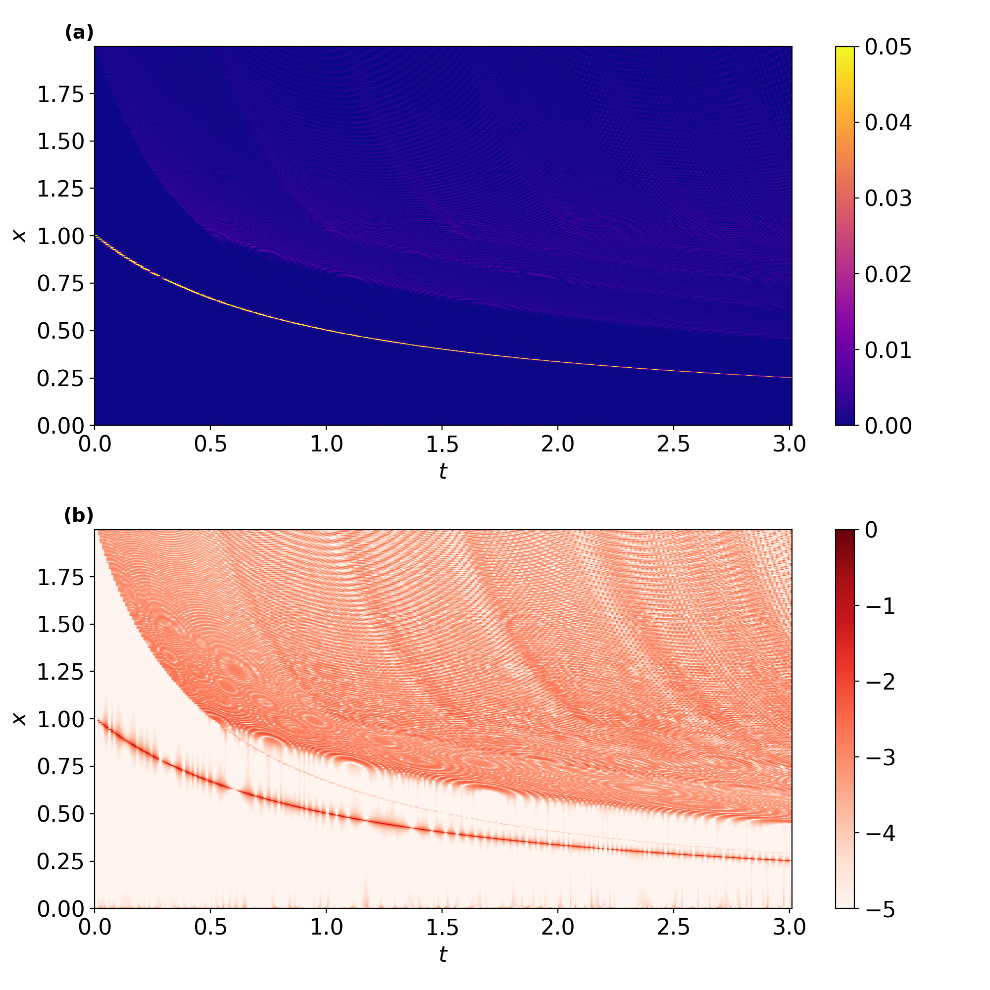
Figure 3: The probability density predicted by KvN mechanics with 10-qubit discretization ($2^{10}$ points in $x\in[0,2.0]$.) Panel (a) shows the evolution of the probability density $\left|\psi\left(x,t\right)\right|^{2}$, visualized as a heatmap. $\left|\psi\right|^{2}\geq 0.05$ is considered as saturated to increase the contrast of the image. The mode of the distribution evolves almost identically with the deterministic solution (cf. analytical solution in Figs. 2 and 4). (b) We plot $\log_{10}\left|\psi\left(x,t\right)\right|^{2}$ as the heatmap to reveal the fine ripple structure resembling a Gibbs-like phenomenon due to the finite dimensional derivative operator.

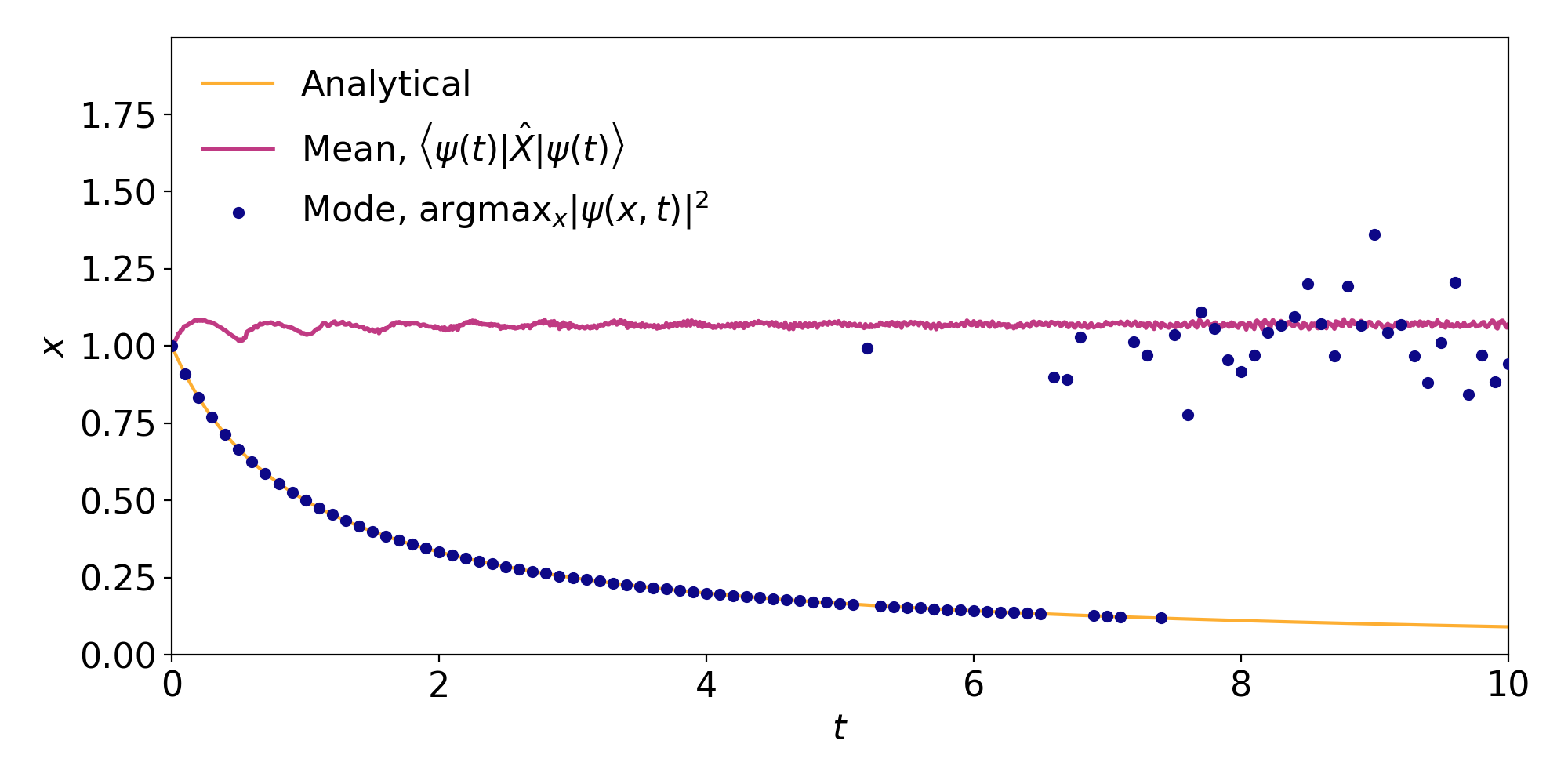
Figure 4: Summary statistics shows that the mode of the probability distribution follows the analytic solution over a short time horizon, $t\lesssim 5$, beyond which the Gibbs-like phenomenon is large enough to disturb the mode into almost random fluctuations. The mean, $\left\langle\psi(t)|\hat{X}|\psi(t)\right\rangle$, on the other hand, is not a useful predictor for all $t\geq 0$.

Example. To illustrate potential problems and pitfalls, we again consider the stylized $\dot{x}=-x^{2}$. We consider a finite domain $x\in\left[0,2\right]$, and only a simple initial condition $x(0)=1$. We partition the system into $2^{10}$ equidistant spatial points and use a discretized wavefunction $\psi=[\psi_{1},\psi_{2},\ldots\psi_{1024}]^{T}.$ The system can be represented as a $10$-qubit quantum state.

We coded the flow operator $\widehat{F(X)}=\hat{X}^{2}$ and $\hat{P}$ operator in the position representation with an FFT-based (Fast Fourier Transform) differentiation. Existing quantum Fourier transformation algorithms enable direct implementation of such FFT-based construction of the $\hat{P}$ operator. After constructing ${H}_{\text{QM}}$ on this discretized lattice, we use scipy.linalg.expm to compute a finite-time propagator $\hat{U}_{\delta}:=\exp(-i{H}_{\text{QM}}\delta)$, with $\delta=0.01$. Again, this is the optimal setting, that we aim to use the most accurate propagator to reveal the finite-size lattice effect. We then use $\hat{U}_{0.01}$ to propagate the wavefunction $\psi$ to $t=10$ iteratively (1000 time steps of size $\delta$).

Figure 3(a) shows the evolution of the probability density $|\psi|^{2}$ up to $t=3$. Although the majority mass of the distribution evolves according to the analytical solution of $\dot{x}=-x^{2}$, noticeable ripples form above the solution $x(t)$. To highlight these ripples, we plot the logarithms of the probability density in Fig. 3(b). Resembling the Gibbs’ phenomenon, these ripples should not be surprising. The eigenfunctions of $\hat{H}$ are all oscillatory in time, but the true dynamics ($\dot{x}=-x$) is dissipative. As a finite discretization restricts us to only $2^{10}$ basis functions, it is not surprising that after a certain time, we lose the ability to use only $2^{10}$ oscillatory modes to approximate and predict long-term behavior. A more thorough analysis of the underlying cause of the Gibbs-like phenomenon can be found in Appendix A.

In Fig. 4, we show that the mode, defined as the lattice point which has the largest amplitude of the wavefunction, evolves almost according to the analytic solution, but only within a finite horizon $t\lesssim 5$. Beyond this horizon, the effect of Gibbs-like phenomena is too strong and we would no longer be able to use the location of the largest amplitude to predict the dynamics.

Interestingly, the expected value of the $\hat{X}$ operator behaves extremely poorly even when the effect of the Gibbs-like phenomenon is small. We remark that all observations are robust to algorithmic parameters, such as the choice of the location of the boundary, number of discretization points, etc., see Supplemental Figs. 7 and 8 with different boundary settings. When changing the initial distribution from $\delta$-like (i.e., probability mass $=1$ on only a specific discretization point) to Gaussian-like, the Gibbs phenomenon is delayed and the prediction horizon by either the mode and expectation value can be improved; see Supplemental Fig. (9).

III.3 Directly solving Liouville equations

The fact that KvN mechanics requires discretization which induces numerical artifacts motivates us to reconsider the problem—if one needs to discretize the space anyway, why not simply come back to the very fundamental problem of solving the Liouville equation by discretization? We propose to discretize the space with countably many points, and formulate the probabilities of the system at each point as a joint distribution with discrete support. A stochastic process can be formulated and described by Chemical Master Equations (CMEs). The joint probability distribution converges to the Liouville equation (3) in the continuum limit via the well-known Kramers–Moyal expansion. The advantage of the CMEs is their transparent resemblance with the original dynamical system. Using CME’s do have a few drawbacks. First, similar to the KvN mechanics, for any finite number of discretization points, intrinsic noise would be introduced and one would need to simulate multiple paths for collecting the statistics. Secondly, the forward propagator $\mathcal{L}^{\dagger}_{\Delta}$ (a discrete approximation of the Liouville operator $\mathcal{L}^{\dagger}$ with spatial grid size $\Delta$) is not a unitary operator, and thus, one cannot simply use the elementary unitary operations in QC for integrating the system forward in time. Instead, we would need to resort to those QC algorithms for solving the general linear equations, noting that CMEs are linear in the variables $p_{j}(t)$. In these probabilistic algorithms, additional sampling is needed to determine the solution. Nevertheless, the numerical accuracy of this discretization scheme seems to be much better than the KvN mechanics.

We finally remark that in terms of the Chemical Master Equations, the adjoint of the forward operator $\mathcal{L}_{\Delta}:=\left(\mathcal{L}_{\Delta}^{\dagger}\right)^{\dagger}$ is the Koopman operator of the approximate process on the finitely many discretization points, and such an adjoint operator is an approximate Koopman operator. When the discretization is dense enough, the analysis of the approximate Koopman operator is similar to a approximate Koopman analysis using Radial Basis Functions Williams et al. (2015b), which have been empirically shown to be practical.

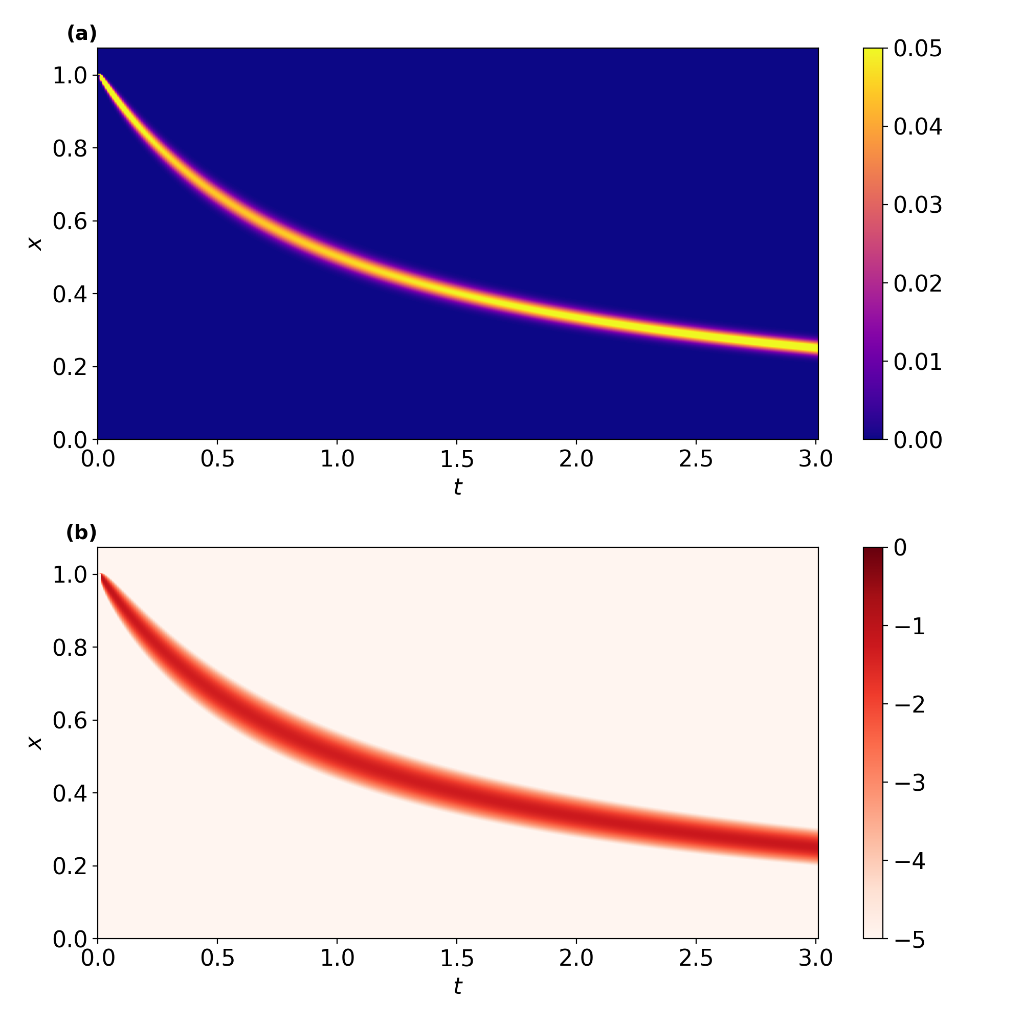
Figure 5: The probability density predicted by the Chemical Master Equation with $2^{10}$ discretization points on a domain $x\in\left[0,2\right]$. Panel (a) shows the evolution of the joint probability distribution $\mathbf{p}(t)$, visualized as a heatmap. $p_{i}(t)\geq 0.05$, $i=1\ldots 1024$ is considered as saturated to increase the contrast of the image. We plot $\log_{10}\mathbf{p}(t)$ as the heatmap in Panel (b), for making comparison to KvN mechanics Fig. (3)(b).

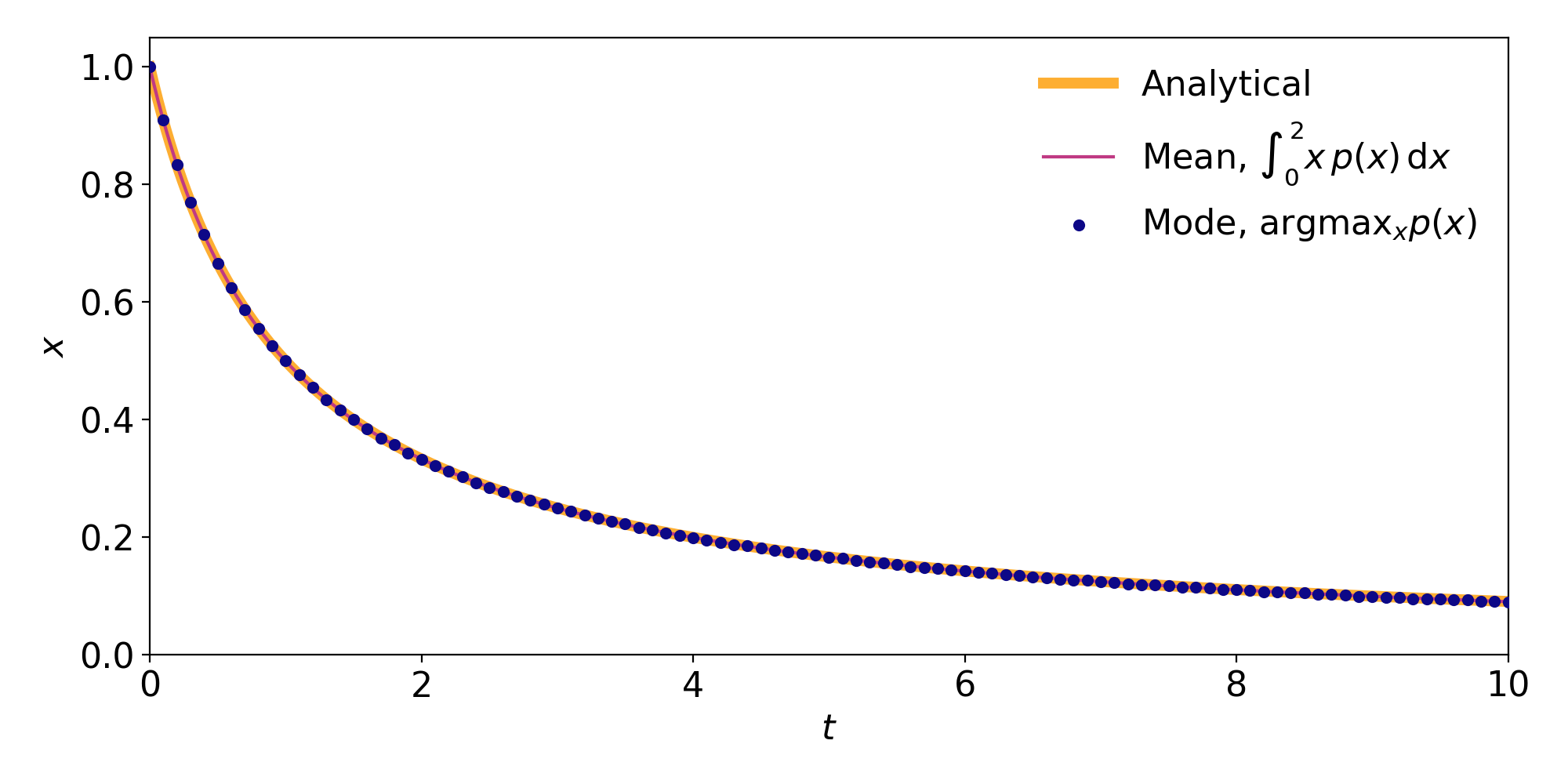
Figure 6: Summary statistics shows that both the mode of the probability distribution and the expectation value follows the analytic solution, showing that the Liouville discretization scheme performs better than the KvN mchanics Fig. 3 on this problem.

Example. In terms of our example $\dot{x}=-x^{2}$, we discretize the space $x\in[0,2]$ into 1024 equidistant points $\left[x_{1},\ldots,x_{1024}\right]^{T}$. We denote the grid size by $\Delta$. The probabilistic system now is captured by 1024 probabilities, $\mathbf{p}(t):=\left[p_{1}(t),\ldots,p_{1024}(t)\right]^{T}$. Since $p(t)$ obeys the linear Liouville equation, we can solve it using the quantum algorithms for linear differential equations Berry (2014); Berry et al. (2017). These algorithms would then output a quantum state whose amplitudes are proportional to the probabilities, i.e. $|\psi\rangle\propto\sum_{n}p_{n}(t)|n\rangle$.  Then, the forward operator $\mathcal{L}_{\Delta}^{\dagger}$ is a sparse Markov matrix, whose entries are defined as

$$\left[\mathcal{L}_{\Delta}^{\dagger}\right]_{i,j}=\left\{\begin{array}[]{cl}-x_{j}^{2}\Delta^{-1}&\text{if }j>0\text{ and }i=j,\\ x_{j}^{2}\Delta^{-1}&\text{if }j>0\text{ and }i=j-1,\\ 0&\text{else.}\end{array}\right.$$ (39)

We can think of the state variable $\mathbf{p}(t)$ as the joint probability distribution of the position of a continuous-time random walk on the lattice. At any time $t$, the walker at $x_{j}$ is only allowed to move to the discretization point to its left $x_{j-1}$ with a transition rate $-x_{j}^{2}$. Then, the CME can be written as a set of 1024 ordinary differential equations, $\mathbf{p}(t)=\mathcal{L}_{\Delta}^{\dagger}\cdot\mathbf{p}(t)$. Again, we used scipy.linalg.expm to calculate the propagator $\exp\left(\delta\mathcal{L}_{\Delta}^{\dagger}\right)$, with $\delta=0.01$. The initial condition is set as $\delta$-distribution-like, i.e., $p_{i}(t)=1$ for $x_{i}=1$ and $0$ otherwise. Analogous to Figs. 3 and 4, we visualize the probability densities in the linear and $\log_{10}$ scale as heat maps in Figs. 5 and 6, showing the improved accuracy for the problem.

We remark that the improvement of the CME approach is specific to the $\dot{x}=-x^{2}$ model. In a parallel analysis on the Van der Pol oscillator presented in Appendix B, we observed that with a finite discretization in phase space, the CME inevitably introduces phase diffusion to the oscillatory dynamics. The KvN mechanics, whose fundamental building blocks are also oscillatory, was seen to perform marginally better than the CME on the Van der Pol oscillator.

The random walk and the corresponding CME may seem to be an ad hoc and heuristic construct for solving the Liouville equation, with the guarantee that the solution of the CME asymptotically (on the infinitely dense grid) converges to the solution of the Liouville equation through the Kramers–Moyal expansion. Another point of view is that the Liouville equation (3) is a hyperbolic conservation law and the CME (39) corresponds to its first-order upwind finite-volume discretization (see, for example, Leveque (2002)). Specifically, we can think of an explicit Euler scheme for solving the Liouville equation as a conservation law for $\rho(x_{i},n\delta)\equiv\rho^{n}_{i}$, evolved over the time step $\delta\ll 1$ as

$$\rho_{i}^{n+1}=\rho_{i}^{n}+\delta\Delta^{-1}\left(\phi_{i+1/2}^{n}-\phi_{i-1/2}^{n}\right),$$ (40)

where $\phi_{i+1/2}^{n}$ is the flux passing through the interface located at $x_{i+1/2}:=\left(x_{i}+x_{i+1}\right)/2$ at time $t=n\delta$. We can choose a specific first-order upwinding scheme $\phi_{i+1/2}^{n}:=x_{i+1}^{2}\rho_{i+1}^{n}$ or using (39), we can write this method as a CME with forward-Euler time integration:

$$\rho_{i}^{n+1}=\rho_{i}^{n}+\delta\left\{\left[\mathcal{L}_{\Delta}^{\dagger}\right]_{i,i+1}\rho^{n}_{i+1}+\left[\mathcal{L}_{\Delta}^{\dagger}\right]_{i,i}\rho^{n}_{i}\right\}.$$ (41)

This discretization is well known to be monotone and thus will not exhibit Gibbs-like numerical artifacts. However, higher-order accurate extensions will result in Gibbs, unless nonlinear feedback is implemented (see Leveque (2002) for more details), and introducing nonlinearity into the numerical method works against our goal of implementation on a QC.

IV Discussion and Summary

We have presented two major motivating results that have driven this perspective. First, we have provided a unified theoretical framework, a “roadmap”, tying together various propositions that can be used to simulate nonlinear dynamical systems on a quantum computer. We believe that classifying and pinpointing potential methods on the “roadmap” is extremely valuable not only to the field of quantum computation, but also to the field of classical dynamical systems. On the one hand, quantum computation could leverage recent advancements in the classical domain, such as various variants of the Dynamic Mode Decomposition and the revived Koopmanism. On the other, classical computational dynamics could leverage the high-dimensional space and faster algorithms that are only feasible in the realm of quantum computing. Our second motivation is to point out potential pitfalls and major technical bottlenecks of these methods in order to provide some guidance for identifying more and less viable directions for further research on quantum algorithms for simulating classical systems.

Both Koopman von Neumann wave mechanics Yu. I. Bogdanov and N. A. Bogdanova (2014); Yu. I. Bogdanov et al. (2019); Joseph (2020) and Carleman linearization Carleman (1932); Kowalski et al. (1991); Liu et al. (2021) have been proposed for the purpose of simulating classical nonlinear dynamics on a quantum computer, leveraging their linear representations. Towards the first aim, we present the duality between the forward representation and backward representation of dynamical systems. We identify a connection between the forward Perron–Frobenius representation and the Koopman von Neumann wave mechanics theory. We also make a connection between the backward Koopman representation and Carleman linearization. We also discuss why the direct nonlinear integration of the flow is not feasible on a quantum computer. Although these are not new theories, we attempted to make the duality clear by juxtaposing the representations in a single article, as most published papers are anchored on only one representation.

With the goal of using Koopman von Neumann wave mechanics to simulate nonlinear systems, we identified that it is a forward, Perron–Frobenius representation, despite its mysterious references to the papers by Koopman and von Neumann, which make use of the backward representation. We discovered that this method is similar to the Proper Orthogonal Decomposition in the classical domain, that the fundamental modes (basis functions) of the dynamics are mutually orthogonal in space, and the eigenvalues are all purely imaginary, leading to wave-like dynamics. We pointed out that the major technical difficulty lies in the fact that discretization can lead to a Gibbs-like phenomenon caused by the under-resolved dynamics on length scales smaller than that of the discretization. Numerical methods that suppress Gibbs are typically nonlinear, even if the original equation being discretized is linear, which is counter to our original goal of solving a linear system on a QC.

Unfortunately, many classical systems, including Hamiltonian ones with chaos, have the feature that the dynamics excites small-scale features in the phase space. Perhaps the most famous example is the Kolmogorov cascade in turbulence. Simulating such systems may require arbitrarily fine discretizations and the question of whether quantum computing can lead to efficiency gains over classical nonlinear integrator operating in the phase-space remains open.

As for the proposition of leveraging Carleman linearization to simulate nonlinear dynamics, we identified that Carleman linearization is a special case of the Koopman representation, in which one uses polynomial functions as the basis functions spanning the Hilbert space. While Liu et al. Liu et al. (2021) showed that it is possible to use Carleman linearization, it is important to point out the limitation that only a special class of dynamical systems is considered in the study: the nonlinearity of the flow example is quadratic, and more importantly, the class of models imposed very strict conditions on the linear stability, i.e. that the system is stable in every direction in the phase space (all eigenvalues of the linearized dynamics are strictly less than zero). As such, any systems with saddles, unstable fixed points, or limit cycles would not fall into this class. For example, both our toy examples, $\dot{x}=-x^{2}$ and the Van der Pol oscillator $\ddot{x}-0.5\left(1-x^{2}\right)\dot{x}+x=0$, are not in the class Liu et al.  analyzed Liu et al. (2021).

The major problem of using Carleman linearization manifests in our numerical illustrations, that there is only a short time horizon during which the linearization would lead to the correct solution. The strict requirement of linear stability in Liu et al. Liu et al. (2021) ensures that errors induced by truncation or projection decay away. For general nonlinear systems, we identify that the major difficulty lies in the identification of closure or projection schemes which are linear in the finite set of functional basis. Unfortunately, such schemes are highly system-dependent and generally unknown a priori without a thorough understanding of the system. Through numerical simulations, we showed that a scheme does exist for the simple equation that we study and can be learned from simulation data via the Extended Dynamic Mode Decomposition Williams et al. (2015a).

Recently, Amini et al. Amini et al. (2021) showed that the error of the Carleman linearization can be bounded exponentially by the truncation order $N$, but this statement does not hold for any arbitrary time. As is clearly described in the paper, provided with the assumption that the flow field can be approximated by a Maclaurin expansion, the error for a sufficiently short horizon is exponentially bounded. However, an estimate of the horizon was not provided. As is shown in our simple numerical examples, undesirable errors can be detrimental in the long time limit even for the stable $\dot{x}=-x^{2}$ system. Thus, it is unlikely that adoption of Carleman linearization for simulating general dynamical systems will be useful when the target is not short-horizon prediction. Furthermore, the number of polynomial basis functions has a stiff scaling with the dimensionality of the phase space and the order of the polynomial (sum of the exponents).

In modern data-driven Koopman learning for dynamical systems, we have learned the valuable lesson that it is challenging to control high-order polynomial basis functions (imagine $x^{100}$ for some $x>1$!) There have been propositions for using radial basis functions or Hermite polynomials Williams et al. (2015a); Alexandre J. Chorin et al. (2002) as the basis functions.

Importantly, it is also well-perceived that the choice of basis functions and the quality of the finite-dimensional approximation strongly depends on the statistical properties (e.g., the ergodic measure) of the specific dynamical system, because the inner product in the Hilbert space $L^{2}\left(\mathbb{R}^{N},\text{d}\mu\right)$ is tied to the statistical properties of the dynamics. Such knowledge can be potentially leveraged to design algorithms for simulating specific dynamical systems on a quantum computer.

If one pursues this route for Koopman representations, for those systems which have finite-dimensional Koopman invariant spaces, knowing the finite set of basis functions which span the invariant subspaces leads to a (potentially nonlinear) transformation of the nonlinear dynamics to a linear and closed one in the Hilbert space, fully solving the problem.

Perhaps the most famous example to this is the Cole–Hopf transform of the nonlinear Burgers’ equation. To this end, we identify the technical difficulty of using a quantum computer lies in the implementation of general nonlinear transformations between the phase space and the observable space. For those systems without finite-dimensional subspaces, how one could improve finite-dimensional approximations for infinite-dimensional dynamics of observables by selecting the optimal set of basis functions remains an open problem.

With our numerical illustrations, we aim to show the simple fact that despite the nice linear properties in these representations—the forward Liouville/Koopman von Neumann mechanics or the backward Koopman representation, there is a trade-off that the operational Hilbert spaces are infinite dimensional. Any reduction to finite dimension inevitably induces numerical errors and the prediction of the dynamics can only be accurate before a finite horizon. There is no free lunch: changing the representation merely changes the formulation of the problem without solving these issues.

In Koopman von Neumann mechanics, a discretization into a finite number of grids in the phase space leads to a finite number of oscillatory modes which are not capable of resolving dynamics below a critical length scale, leading to a Gibbs-like phenomenon.

Lloyd et al. Lloyd et al. (2020) takes a different approach to solving nonlinear differential equations based on the simulation of nonlinear Schrödinger equations. This entails designing an interacting many-body system evolving according to the standard Schrödinger equation such that the dynamics of each of the identical individual particles is described by a nonlinear Schrödinger equation in the thermodynamic limit (infinitely many particles). Finite many-body systems of this sort can be efficiently simulated with quantum computers. However, note that for the nonlinear Hartree equation, Gokler Gokler (2020) derived an upper bound on the error of the mean field approach that for a finite number of particles grows exponentially in time. This behavior of the upper bound is analogous to that for the truncated Carleman approach Forets and Pouly (2017). Whether in general the mean-field approach has a corresponding finite-time horizon for accurate solutions is a subject for future work. All of the methods considered here, however, have similar issues related to discretization of some sort. Since the method of Lloyd et al. (2020) does not evolve observables, it is evidently a Perron-Frobenius method. Moreover, it has a significant advantage over the Perron-Frobenius methods discussed in this work (KvN and the direct method of Sections III.2 and III.3) because the encoding of the mean-field is much more efficient and could allow for exponentially finer lattices for fluid simulations.

In the Carleman and the more general Koopman representation, the choice of a finite number of basis functions leads to inevitable projection or truncation of the exponentially resolved observable dynamics. Without a data-driven approach to learning the projection operator from data, naïve truncations can even lead to diverging predictions.

Notwithstanding the above considerations, our perspective on using quantum computing to simulate nonlinear dynamical systems remains conservatively optimistic for two reasons. First, we are hopeful that the infinite-dimensional spaces can be reasonably approximated by a quantum computational system, whose state space is also a Hilbert space whose dimension is exponential in the number of qubits. Secondly, we are hopeful that the more efficient quantum linear solver can significantly enhance the integration process in comparison to classical linear solvers.

Challenges exist of finding general nonlinear transformations Holmes et al. (2021) for those systems with closed Koopman invariant spaces, or devising finite-state approximations and estimating their errors for general systems. The solutions to these challenges are likely to depend on which nonlinear system one is studying.

V Acknowledgements

YTL appreciates useful discussions with Francesco Caravelli. This work was supported by the Beyond Moore’s Law project of the Advanced Simulation and Computing Program at Los Alamos National Laboratory managed by Triad National Security, LLC, for the National Nuclear Security Administration of the U.S. Department of Energy under contract 89233218CNA000001.

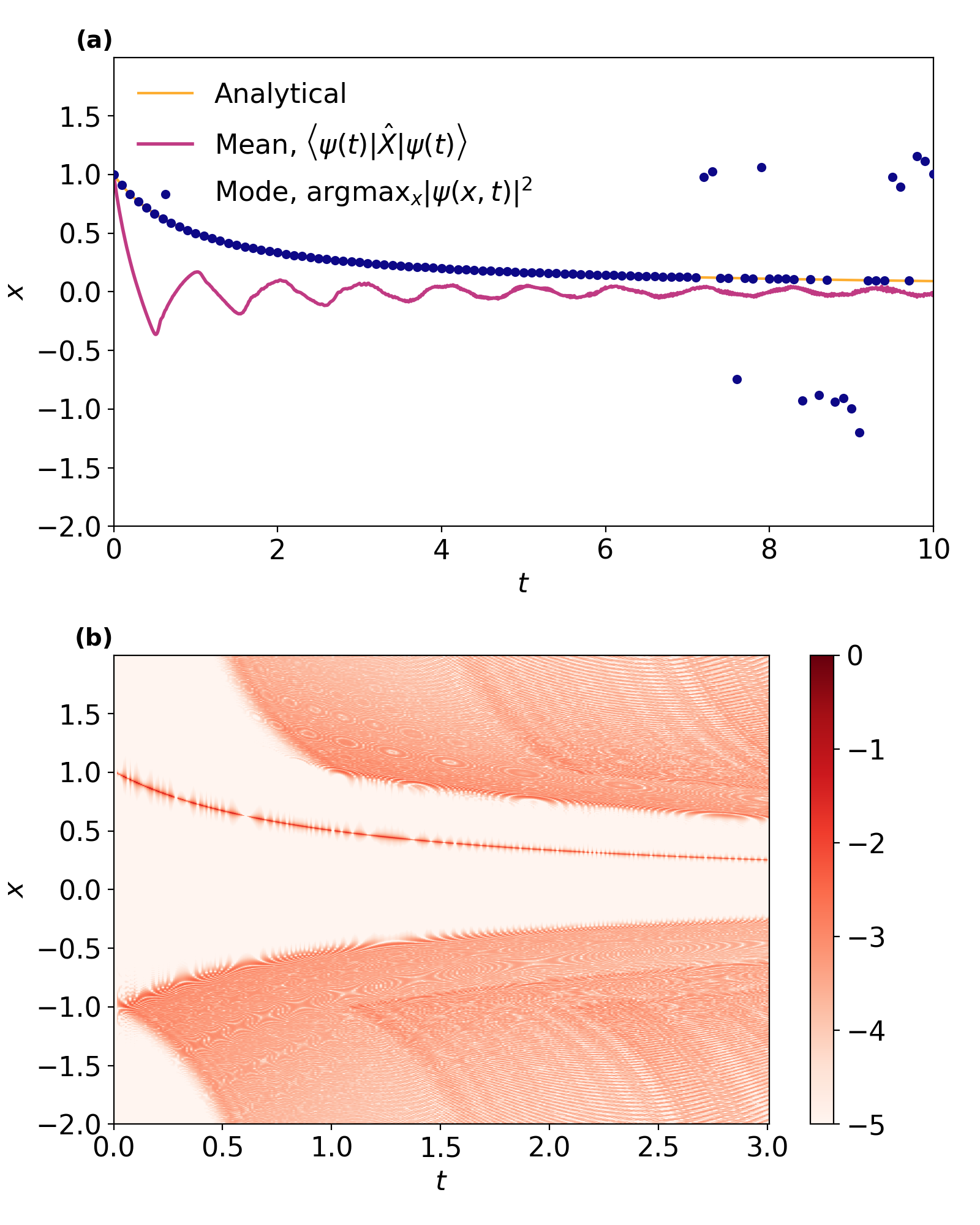
Figure 7: KvN mechanics for the $\dot{x}=-x^{2}$ model. The domain is extended to $[-2,2]$, with with $2^{11}$ discretization points. (a) the summary statistics (cf. Fig. 4); (b) The base-10 logarithm of the probability density (cf. Fig. 3(b)).

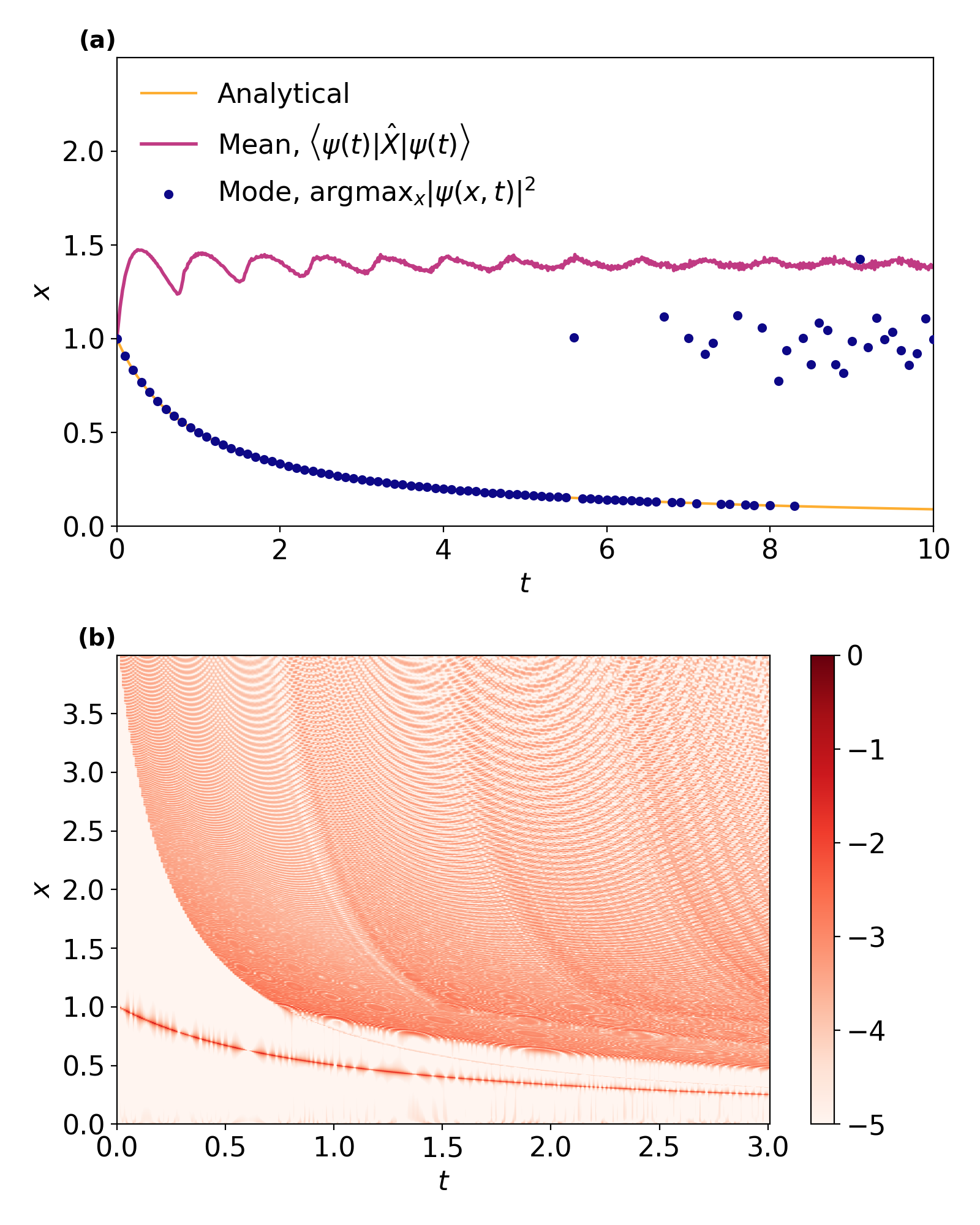
Figure 8: KvN mechanics for the $\dot{x}=-x^{2}$ model. The domain is extended to $[0,4]$, with $2^{11}$ discretization points. (a) the summary statistics (cf. Fig. 4); (b) The base-10 logarithm of the probability density (cf. Fig. 3(b)).

Appendix A Effects of boundary and initial condition in KvN mechanics

We wondered if the ripples (Gibbs-like phenomenon) could be resolved by changing the boundary conditions and/or initial distributions. Analyses were performed by changing the domain of the system from $x\in\left[0,2\right]$, specified in the main text, to $[-2,2]$ and $[0,4]$. To accommodate the extended domains, in both cases, we discretized the system into $2^{11}$ points. The summary statistics (cf. Fig. 4) and the probability density in the base-10 logarithmic space (cf. Fig. 3(b)) are presented in Figs. 7 and Figs. 8. We conclude that the observations presented in the main text are robust to the change of the boundary setting.

To evaluate the effect of initial conditions, motivated by the physical constraint that we cannot initiate a $\delta$-distribution on a quantum system with continuum state space, we initiated a smoothed initial condition centered at $x=1$, shown in the inset of Fig. 9. We observed that the Gibbs-like phenomenon was delayed, leading to a short horizon ($t\leq 1$) in which both the first moment and the mode of the probability distribution can reasonably approximate the analytical solution. The horizon of the mode prediction is extended to $t>10$ (Cf. $t\approx 5$ in Fig. 4). With a wider initial distribution (inset in Fig. 10), we can achieve an even longer horizon before which the first moment and the mode of the discretized KvN wavefunction reasonably approximates the analytical solution, see the summary statistics in Fig. 10(a) and the joint probability distribution in the base-10 logarithmic scale in Fig. 10(b). In Fig. 10(c), we calculated the standard deviation of the distribution, showing the underlying cause of the Gibbs-like phenomenon. Because the dynamics $\dot{x}=-x^{2}$ has a global fixed point $x=0$, the probability distribution will eventually converge to this zero-measure point as $t\rightarrow\infty$. Thus, in the long-time limit, the majority of the probability mass is inevitably “pinched” into an interval that is smaller than the finite grid can resolve. We observe that soon after the standard deviation of the probability distribution decreases down to less than the grid-size $\Delta$, the solution became oscillatory: the standard deviation rebounded and started to increase. Noticeable Gibbs-like phenomena occurred soon after the rebound (see Fig. 10(b), $t\approx 3.5$) and destroys the predictions.

We remark that the Gibbs-like phenomenon, well-known in spectral analysis Gottlieb and Orszag (1977); Harten (1996); Boyd (2000) is purely classical and due to under-resolved finite-dimensional projection of an infinite-dimensional space.

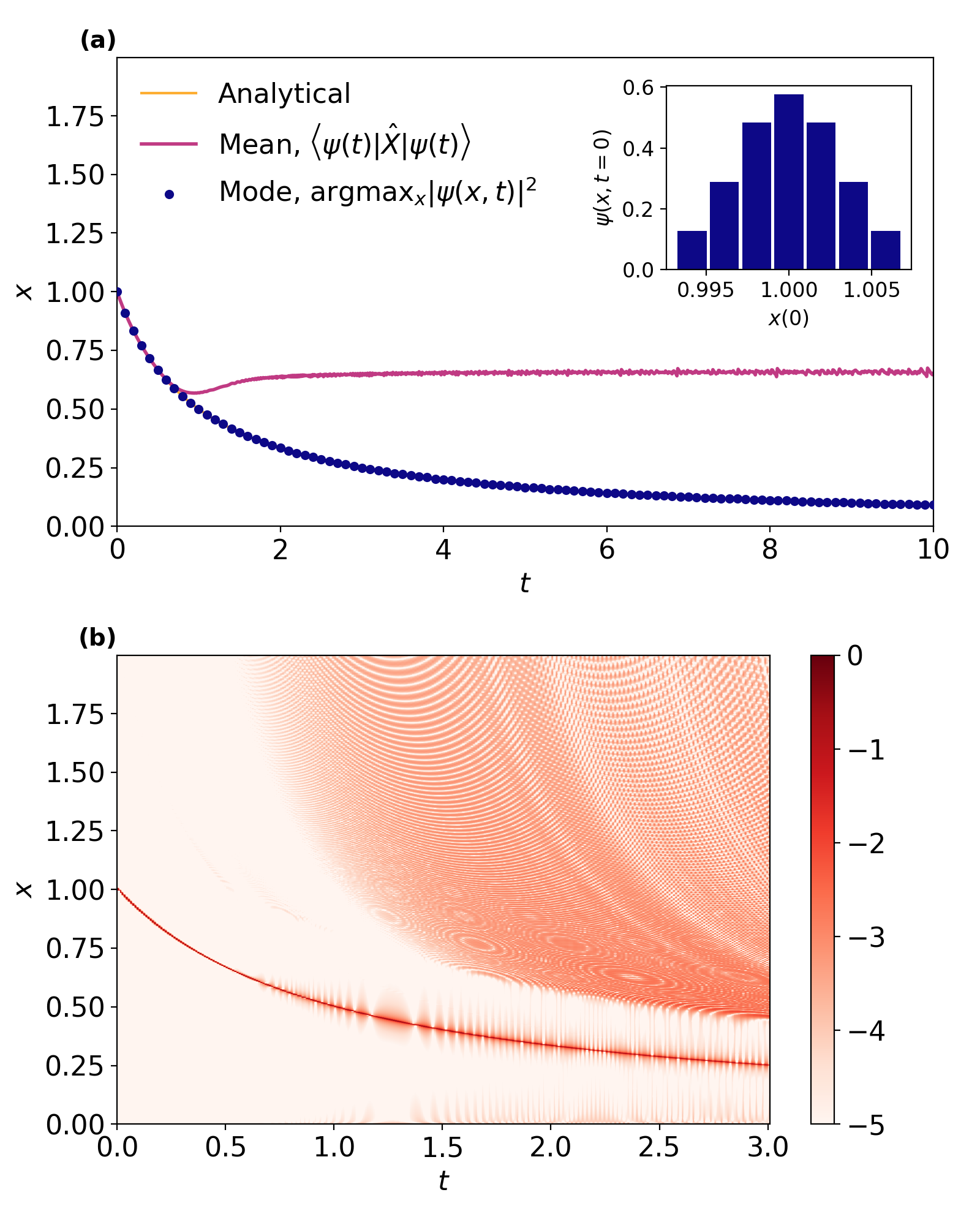
Figure 9: KvN mechanics for the $\dot{x}=-x^{2}$ model. Instead of $\delta$-like initial distribution, we put a Gaussian-like, 7-point distribution centered at $x=1$. (a) The summary statistics (cf. Fig. 4). We plot the initial wavefunction in the inset; (b) The base-10 logarithm of the probability density (cf. Fig. 3(b)).

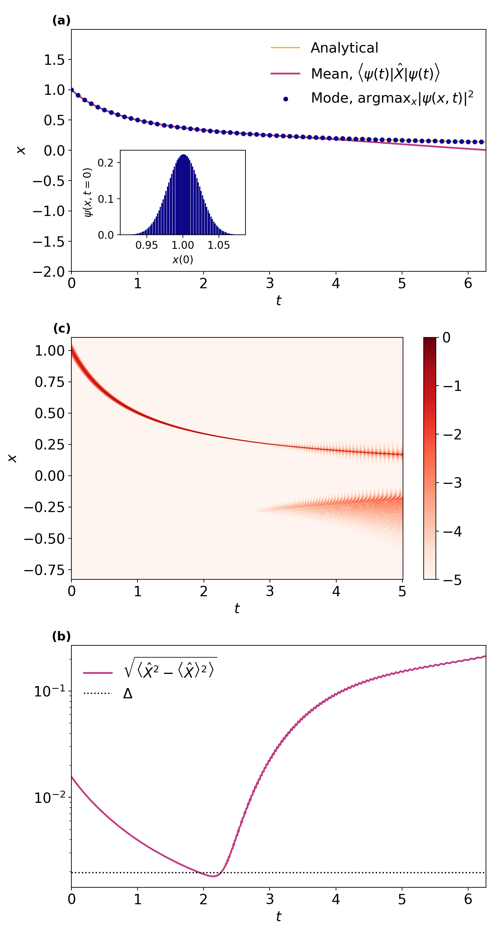
Figure 10: KvN mechanics for the $\dot{x}=-x^{2}$ model. Instead of $\delta$-like initial distribution, we put a Gaussian-like, 80-point distribution centered at $x=1$. (a) The summary statistics (cf. Fig. 4). We plot the initial wavefunction in the inset; (b) The standard deviation of the distribution as a function of time; (c) The base-10 logarithm of the probability density (cf. Fig. 3(c)).

Figure 11: Error analysis: (a-d) correspond to Figs. 3, 5, 9, and 10. The integrated probability density in the interval $(x_{\text{analytical}}(t)-\varepsilon,x_{\text{analytical}}(t)+\varepsilon)$ is plotted against evolution time. Hence $p_{\varepsilon}$ can be interpreted as the probability of obtaining an answer within error $\varepsilon$ if a measurement in the computational basis is performed on the quantum state that encodes the solution to the dynamical system at that time.

We now observe an interesting trade-off: in comparison to a sharper (e.g., $\delta$-like) distribution, a wider initial distribution has a further prediction horizon but with a larger variance. To determine the summary statistics, e.g., the first moment of the probability distribution, the system with a wider initial distribution must require more samples. The observation seems to suggest that, at least for this system, one would choose the variance of the initial distribution to be such that at the prediction time, the variance of the evolving distribution is about $\Delta^{2}$. A larger than $\Delta^{2}$ variance at the prediction time would require additional samples to determine the summary statistics. A smaller than $\Delta^{2}$ variance would invoke the under-resolving problem. A certain optimization of the initial distribution, conditioned on the prediction time, is needed.

Finally, we remark that the problem is generic if the dynamics has any “pinching”, i.e., compression of the probability distribution in any direction in the phase space. Notice that even Hamiltonian systems may have such a feature: they are volume-preserving, but they can have a flow compressing in one direction and expanding in another direction. For those systems with invariant manifolds, such as fixed points and limit cycles, KvN mechanics with discretization does not seem to be a stable and scalable method for predicting long-time behaviors near those manifolds.

Appendix B An alternative model: Van der Pol oscillator

To showcase that our observations are not conditioned on the particular choice of the model presented in the main text ($\dot{x}=-x^{2}$; see §III.3), we performed a parallel analysis on the Van der Pol oscillator. The evolutionary equations of the two-dimensional system are:

$$\dot{x}={} F_{x}(x,y):=y,$$ (42a)

$$\dot{y}={} F_{y}(x,y):=-x+\mu\left(1-x^{2}\right)y.$$ (42b)

The Van der Pol oscillator has a globally stable limit cycle, provided $\mu>0$. In this analysis, we fixed the model parameter $\mu=0.5$. The initial condition of the system is an arbitrary point near the stable limit cycle, obtained by integrating the system forward in time for a sufficient amount of time ($t=100$). We remark that the choice of $\mu$ led to a less stiff dynamical system. When we changed to $\mu=10$, which corresponds to a very stiff dynamical system, the methods below did not seem to solve the problem due to numerical instability.

Numerical solution. The Van der Pol oscillator does not have an analytical solution. To set up the baseline, we used the general-purposed scipy.optimize.solve_ivp with lsoda to obtained the numerical solution. The absolute and relative errors are both set at a stringent $10^{-10}$.

Carleman linearization. We perform the Carleman linearization on the set of polynomial functions $g_{m,n}:=x^{m}y^{n}$. It is straightforward to show that the evolutionary equations are:

$$\dot{g}_{m,n}={} mg_{m-1,n+1}-ng_{m+1,n-1}$$

$$+\mu n\left(g_{m,n}-g_{m+2,n}\right).$$ (43)

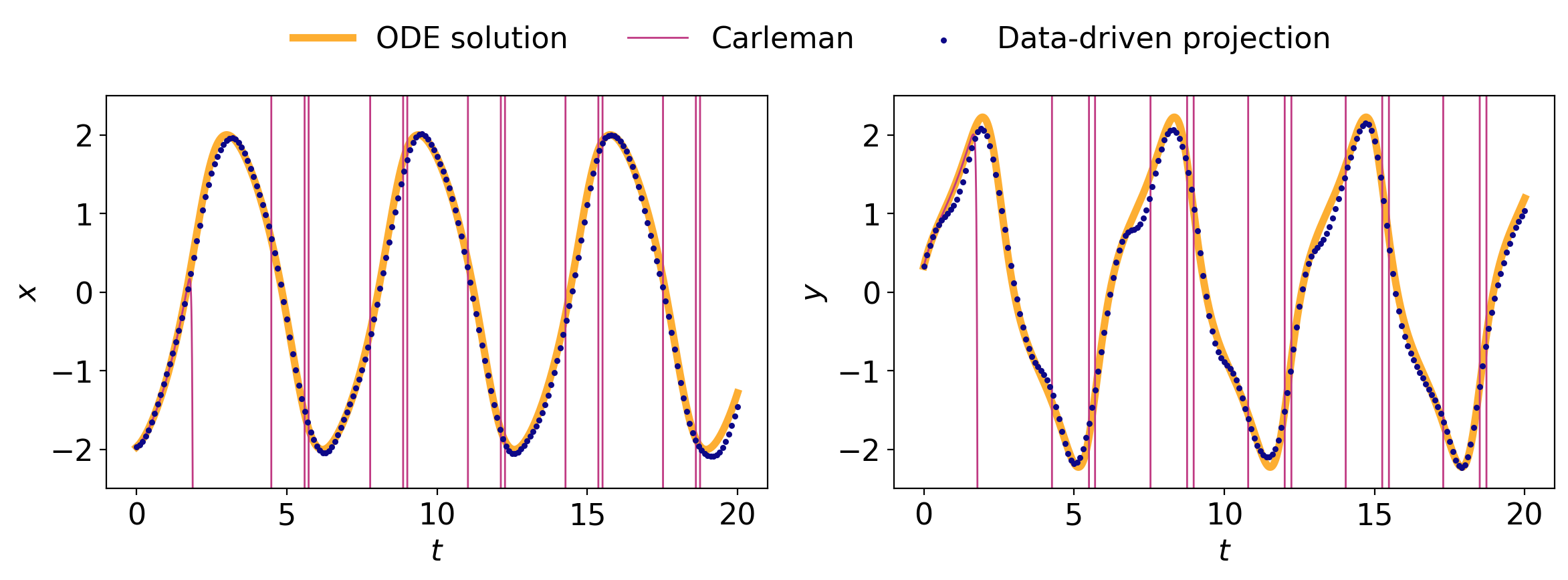
Figure 12: Predictions by the Carleman linearization and approximate Koopman operator learned from EDMD for the Van der Pol oscillator.

The truncation scheme is devised as follows. First, we only consider a polynomial order of $m+n\leq 49$. Thus, the state space leads to 1,275 functions. By observing the evolutionary equation (42), we know that the equation $g_{m,n}$ can only be closed if the $g$’s on the RHS are in the set in the state space. The problematic ones are the $g_{m+2,n}$ when $m+n\geq 48$. We assume that $\dot{g}_{m,n}=0$ if $m+n\geq 48$ to close the system. We also tried different orders and truncation schemes and observed equally poor prediction [data not shown], as seen in Fig. 12.

Data-driven projection. To showcase that there exists an approximate Koopman operator acting on a functional subspace in $\mathcal{L}^{2}\left(\mathbb{R}^{n},\rho_{0}\left(x\right)\text{d}x\right)$, which reasonably approximates the dynamics, we consider the above polynomial functions up to $m+n\leq 4$. This leads to a 10-dimensional functional space. To learn the approximate Koopman operator, we use the numerical solution on a uniform temporal grid with $\delta=0.002$ from $t=0$ to $t=20$ (i.e., 10,000 snapshots of the system). We use the polynomials ($m+n\leq 4$) as the dictionary to perform EDMD and learn the one-step approximate Koopman operator in the sub-functional space spanned by the dictionary. The learned $\mathbf{K}_{\delta=0.002}$ is then used to propagate the initial condition recursively. Both state variables $x$ and $y$, already in this dictionary as $g_{1,0}$ and $g_{0,1}$, are reported in Fig. 12.

KvN mechanics. We partition the domain $\left(x,y\right)\in\left[-4,4\right]\times\left[-3,3\right]$ to $128\times 128$ discretized points. The operators $-i\partial_{x}$ and $-i\partial_{y}$ are constructed by FFT-based (Fast Fourier Transform) differentiation. We used scipy.linalg.expm to exponentiate the constructed KvN Hamiltonain and obtain finite-time propagator, $\exp\left(-i\mathcal{H}_{\text{KvN}}\delta\right)$. We chose $\delta=0.01$. The system is evolved forward in time until $t=12$ (total 1,200 time steps). The results are presented in Fig. 13.

Directly solving Liouville equations. We partition the domain $\left(x,y\right)\in\left[-4,4\right]\times\left[-3,3\right]$ to $128\times 128$ discretized points. Denote the coordinates of these discretized points by $(x_{j},y_{k})$, $j,k\in\left\{1,\ldots,128\right\}$, we consider a random walk following the below rules on the lattice grid:

$$\left(x_{j},y_{k}\right)\xrightarrow{\frac{\left|F_{x}\left(x_{j},y_{k}\right)\right|}{\Delta_{x}}}\left(x_{j+\text{sign}\left(F_{x}\left(x_{j},y_{k}\right)\right)},y_{k}\right),$$ (44a)

$$\left(x_{j},y_{k}\right)\xrightarrow{\frac{\left|F_{y}\left(x_{j},y_{k}\right)\right|}{\Delta_{y}}}\left(x_{j},y_{k+\text{sign}\left(F_{y}\left(x_{j},y_{k}\right)\right)}\right).$$ (44b)

Here, $F_{x}$ and $F_{y}$ are the flow defined in (42). The transition rates are annotated in above the arrows. We also truncate the reactions so that the random walker is always confined on the $128\times 128$ lattice. The joint probability distribution, $p_{i,j}\left(t\right)=\mathbb{P}\left\{\text{The random walker is at }x_{j},y_{k}\text{ at time }t\right\}$, $i,j\in\left\{1,\ldots 128\right\}$ follows a CME, which is our object of interest. By stacking up the probabilities into a $16384\times 1$ column vector $\mathbf{p}(t)$, the CME is $\dot{\mathbf{p}}\left(t\right)=\mathcal{L}_{\Delta}^{\dagger}\cdot\mathbf{p}\left(t\right)$. We then solve the operator $\exp\left(\delta\mathcal{L}_{\Delta}^{\dagger}\right)$ by exponentiation of the matrix, using scipy.linalg.expm, for forward propagating the initial density. Similar to the setting in the KvN mechanics, we chose $\delta=0.01$ and propagate the initial state 1,200 steps.

The results, presented in Fig. 14, showed a clear signature of stochastic phase diffusion where the probability density is dispersed near the stable limit cycle. For this system and with this parametrization ($\mu=0.5$), the mode of the KvN mechanics (Figs. 13(c) and (f)) is almost identical to the true solution and is more accurate than that of the CME (Figs. 14(c) and (f)), which suffered from phase diffusion. However, we observed that the first moments of the CME are more reliable than that of the KvN mechanics, which suffers from the Gibbs-like phenomena (Figs. 13)(a-b) and (d-e).

Following the approach that led to (40), a first-order upwind discretization of Liouville dynamics for the Van der Pol oscillator may be written as

$$\rho_{j,k}^{n+1}=\rho_{j,k}^{n}-\frac{\delta}{\Delta_{x}}\left[\left(F_{x}\rho\right)^{n}_{j+1/2,k}-\left(F_{x}\rho\right)^{n}_{j-1/2,k}\right]\\ -\frac{\delta}{\Delta_{y}}\left[\left(F_{y}\rho\right)^{n}_{j,k+1/2}-\left(F_{y}\rho\right)^{n}_{j,k-1/2}\right],$$ (45)

where the interface fluxes are defined by

$$\left(F_{x}\rho\right)^{n}_{j+1/2,k}={} \left(\phi_{R}\right)^{n}_{j+1/2,k}+\left(\phi_{L}\right)^{n}_{j+1/2,k},$$ (46a)

$$\left(\phi_{R}\right)^{n}_{j+1/2,k}:={} \left\{\begin{array}[]{cl}\frac{\left(F_{x}\right)_{i,j}}{\Delta_{x}}\rho\left(x_{i},y_{j},t\right)&\text{ if }\left(F_{x}\right)_{i,j}>0\\ 0&\text{ else,}\end{array}\right.$$ (46d)

$$\left(\phi_{L}\right)^{n}_{j+1/2,k}:={} \left\{\begin{array}[]{cl}\frac{\left(F_{x}\right)_{i+1,j}}{\Delta_{x}}\rho\left(x_{i+1},y_{j},t\right)&\text{ if }\left(F_{x}\right)_{i+1,j}<0\\ 0&\text{ else,}\end{array}\right.$$ (46g)

where $$\phi_{R} \phi_{L} \left(j+1/2,k\right) \left(F_{x}\right)_{i,j}:=F_{x}\left(x_{i},y_{j}\right)$$ and are right- and left-passing fluxes crossing the same interface , and

$$\left(F_{y}\rho\right)^{n}_{j,k+1/2}={} \left(\phi_{U}\right)^{n}_{j,k+1/2}+\left(\phi_{D}\right)^{n}_{j,k+1/2},$$ (46h)

$$\left(\phi_{U}\right)^{n}_{j,k+1/2}:={} \left\{\begin{array}[]{cl}\frac{\left(F_{y}\right)_{i,j}}{\Delta_{y}}\rho\left(x_{i},y_{j},t\right)&\text{ if }\left(F_{y}\right)_{i,j}>0\\ 0&\text{ else,}\end{array}\right.$$ (46k)

$$\left(\phi_{D}\right)^{n}_{j,k+1/2}:={} \left\{\begin{array}[]{cl}\frac{\left(F_{y}\right)_{i,j+1}}{\Delta_{y}}\rho\left(x_{i},y_{j+1},t\right)&\text{ if }\left(F_{y}\right)_{i,j+1}<0\\ 0&\text{ else,}\end{array}\right.$$ (46n)

where $\phi_{U}$ and $\phi_{D}$ are upward- and downward-passing fluxes crossing the same interface $\left(j,k+1/2\right)$, and $\left(F_{y}\right)_{i,j}:=F_{y}\left(x_{i},y_{j}\right)$. Our choices here for the finite-volume discretization, Eqs. (46a) to (46n), led to an evolutionary equation (45) that matches the CME describing the probability distribution of the random walk exactly (44).

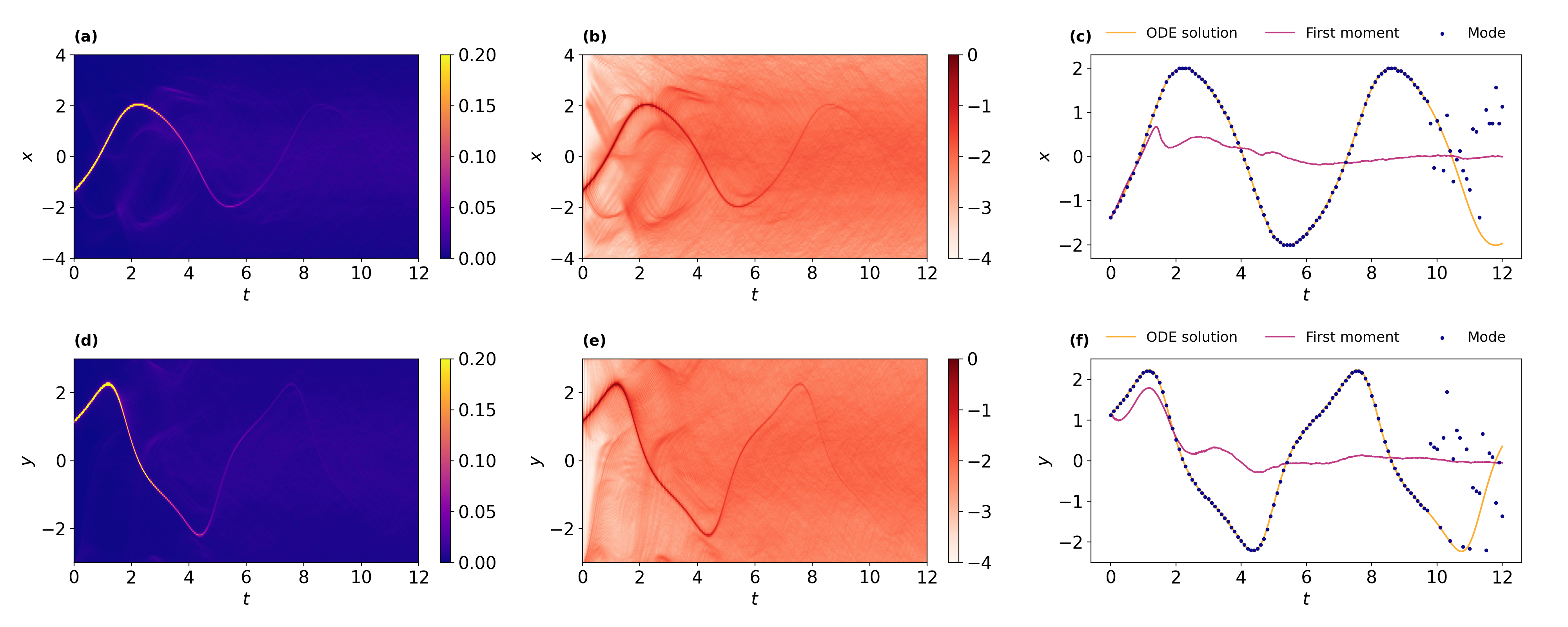
Figure 13: KvN mechanics of the Van der Pol oscillator.

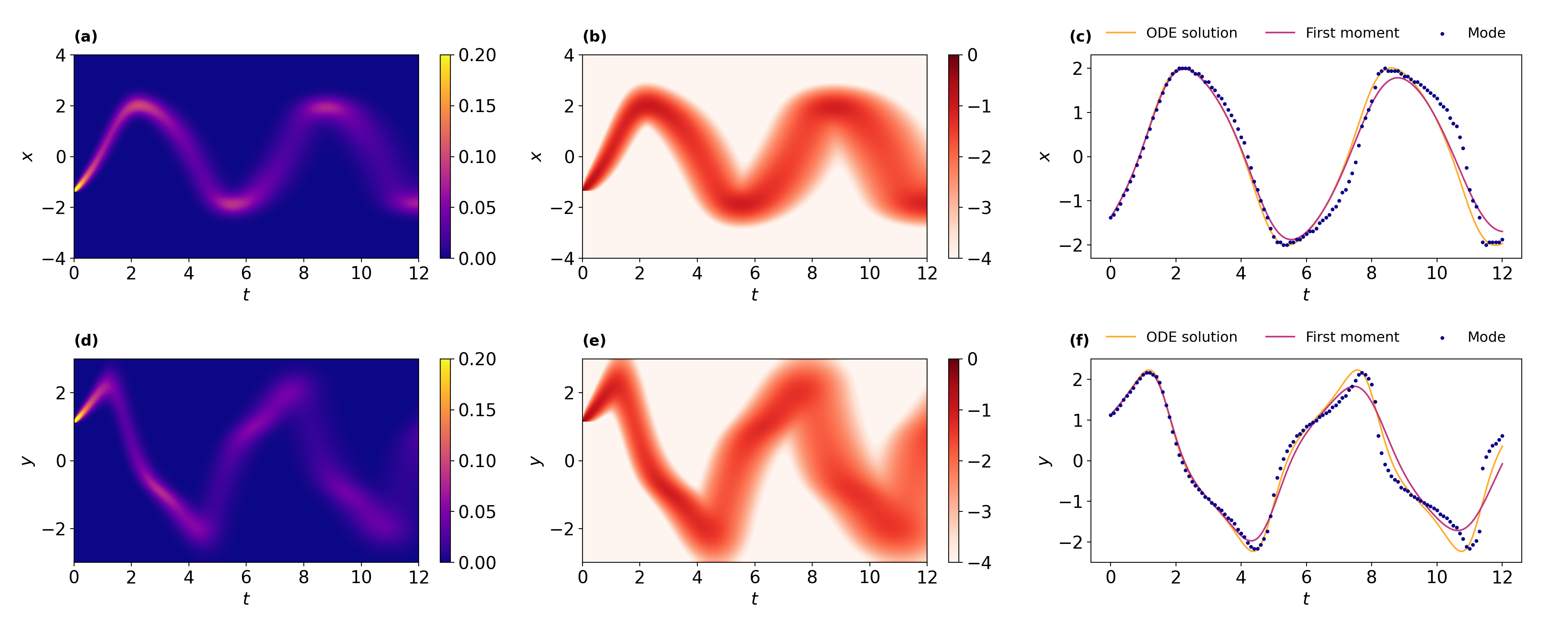
Figure 14: CME approximating the Liouville dynamics of the Van der Pol oscillator.

References

- Benioff (1980) Paul Benioff, “The computer as a physical system: A microscopic quantum mechanical hamiltonian model of computers as represented by turing machines,” Journal of statistical physics 22, 563–591 (1980).
- Feynman (2018) Richard P Feynman, “Simulating physics with computers,” in Feynman and computation (CRC Press, 2018) pp. 133–153.
- Lloyd (1996) Seth Lloyd, “Universal quantum simulators,” Science , 1073–1078 (1996).
- Yoshida (1990) Haruo Yoshida, “Construction of higher order symplectic integrators,” Physics letters A 150, 262–268 (1990).
- Boghosian and Taylor IV (1998) Bruce M Boghosian and Washington Taylor IV, “Simulating quantum mechanics on a quantum computer,” Physica D: Nonlinear Phenomena 120, 30–42 (1998).
- Sornborger and Stewart (1999) AT Sornborger and Ewan D Stewart, “Higher-order methods for simulations on quantum computers,” Physical Review A 60, 1956 (1999).
- Berry et al. (2015) Dominic W Berry, Andrew M Childs, Richard Cleve, Robin Kothari, and Rolando D Somma, “Simulating hamiltonian dynamics with a truncated taylor series,” Physical review letters 114, 090502 (2015).
- Low and Chuang (2019) Guang Hao Low and Isaac L Chuang, “Hamiltonian simulation by qubitization,” Quantum 3, 163 (2019).
- Harrow et al. (2009) Aram W Harrow, Avinatan Hassidim, and Seth Lloyd, “Quantum algorithm for linear systems of equations,” Physical review letters 103, 150502 (2009).
- Ambainis (2012) Andris Ambainis, “Variable time amplitude amplification and quantum algorithms for linear algebra problems,” in Proceedings of the 29th International Symposium on Theoretical Aspects of Computer Science (2012) pp. 636–647.
- Childs et al. (2017) Andrew Childs, Robin Kothari, and Rolando D. Somma, “Quantum linear systems algorithm with exponentially improved dependence on precision,” SIAM J. Comp. 46, 1920 (2017).
- Subaşı et al. (2019) Yiğit Subaşı, Rolando D Somma, and Davide Orsucci, “Quantum algorithms for systems of linear equations inspired by adiabatic quantum computing,” Physical review letters 122, 060504 (2019).
- An and Lin (2019) Dong An and Lin Lin, “Quantum linear system solver based on time-optimal adiabatic quantum computing and quantum approximate optimization algorithm,” arXiv:1909.05500 (2019).
- Berry (2014) Dominic W Berry, “High-order quantum algorithm for solving linear differential equations,” Journal of Physics A: Mathematical and Theoretical 47, 105301 (2014).
- Berry et al. (2017) Dominic W Berry, Andrew M Childs, Aaron Ostrander, and Guoming Wang, “Quantum algorithm for linear differential equations with exponentially improved dependence on precision,” Communications in Mathematical Physics 356, 1057–1081 (2017).
- Costa et al. (2019) Pedro CS Costa, Stephen Jordan, and Aaron Ostrander, “Quantum algorithm for simulating the wave equation,” Physical Review A 99, 012323 (2019).
- Cao et al. (2013) Yudong Cao, Anargyros Papageorgiou, Iasonas Petras, Joseph Traub, and Sabre Kais, “Quantum algorithm and circuit design solving the poisson equation,” New Journal of Physics 15, 013021 (2013).
- Sinha and Russer (2010) Siddhartha Sinha and Peter Russer, “Quantum computing algorithm for electromagnetic field simulation,” Quantum Information Processing 9, 385–404 (2010).
- Engel et al. (2019) Alexander Engel, Graeme Smith, and Scott E Parker, “Quantum algorithm for the vlasov equation,” Physical Review A 100, 062315 (2019).
- Leyton and Osborne (2008) Sarah K Leyton and Tobias J Osborne, “A quantum algorithm to solve nonlinear differential equations,” arXiv preprint arXiv:0812.4423 (2008).
- Joseph (2020) Ilon Joseph, “Koopman–von Neumann approach to quantum simulation of nonlinear classical dynamics,” Physical Review Research 2, 043102 (2020).
- Dodin and Startsev (2021) Ilya Y Dodin and Edward A Startsev, “On applications of quantum computing to plasma simulations,” Physics of Plasmas 28, 092101 (2021).
- Giannakis et al. (2020) Dimitrios Giannakis, Abbas Ourmazd, Joanna Slawinska, and Joerg Schumacher, “Quantum compiler for classical dynamical systems,” arXiv preprint arXiv:2012.06097 (2020).
- Liu et al. (2021) Jin-Peng Liu, Herman Øie Kolden, Hari K Krovi, Nuno F Loureiro, Konstantina Trivisa, and Andrew M Childs, “Efficient quantum algorithm for dissipative nonlinear differential equations,” Proceedings of the National Academy of Sciences 118 (2021).
- Lloyd et al. (2020) Seth Lloyd, Giacomo De Palma, Can Gokler, Bobak Kiani, Zi-Wen Liu, Milad Marvian, Felix Tennie, and Tim Palmer, “Quantum algorithm for nonlinear differential equations,” arXiv preprint arXiv:2011.06571 (2020).
- Engel et al. (2021) Alexander Engel, Graeme Smith, and Scott E Parker, “Linear embedding of nonlinear dynamical systems and prospects for efficient quantum algorithms,” Physics of Plasmas 28, 062305 (2021).
- Xu et al. (2018) Guanglei Xu, Andrew J. Daley, Peyman Givi, and Rolando D. Somma, “Turbulent mixing simulation via a quantum algorithm,” AIAA Journal 56, 687–699 (2018), https://doi.org/10.2514/1.J055896 .
- Loh Jr et al. (1990) EY Loh Jr, JE Gubernatis, RT Scalettar, SR White, DJ Scalapino, and RL Sugar, “Sign problem in the numerical simulation of many-electron systems,” Physical Review B 41, 9301 (1990).
- Van Bemmel et al. (1994) HJM Van Bemmel, DFB Ten Haaf, W Van Saarloos, JMJ Van Leeuwen, and Guozhong An, “Fixed-node quantum monte carlo method for lattice fermions,” Physical review letters 72, 2442 (1994).
- Troyer and Wiese (2005) Matthias Troyer and Uwe-Jens Wiese, “Computational complexity and fundamental limitations to fermionic quantum monte carlo simulations,” Physical review letters 94, 170201 (2005).
- Klus et al. (2018) Stefan Klus, Feliks Nüske, Péter Koltai, Hao Wu, Ioannis Kevrekidis, Christof Schütte, and Frank Noé, “Data-Driven Model Reduction and Transfer Operator Approximation,” Journal of Nonlinear Science 28, 985–1010 (2018).
- Koopman (1931) B O Koopman, “Hamiltonian systems and transformation in Hilbert space,” Proceedings of the National Academy of Sciences 17, 315–318 (1931).
- Koopman and v. Neumann (1932) B O Koopman and J v. Neumann, “Dynamical systems of continuous spectra,” Proceedings of the National Academy of Sciences 18, 255–263 (1932).
- Mezić (2005) Igor Mezić, “Spectral Properties of Dynamical Systems, Model Reduction and Decompositions,” Nonlinear Dynamics 41, 309–325 (2005).
- Ale et al. (2013) Angelique Ale, Paul Kirk, and Michael P. H. Stumpf, “A general moment expansion method for stochastic kinetic models,” The Journal of Chemical Physics 138, 174101 (2013).
- Schnoerr et al. (2015) David Schnoerr, Guido Sanguinetti, and Ramon Grima, “Comparison of different moment-closure approximations for stochastic chemical kinetics,” The Journal of Chemical Physics 143, 185101 (2015).
- Carleman (1932) Torsten Carleman, “Application de la théorie des équations intégrales linéaires aux systèmes d’équations différentielles non linéaires,” Acta Math. 59, 63–87 (1932).
- Kowalski et al. (1991) Krysztof L Kowalski, W. H Steeb, and K Kowalksi, Nonlinear Dynamical Systems and Carleman Linearization. (World Scientific Publishing Company, Singapore, 1991).
- Lin et al. (2021) Yen Ting Lin, Yifeng Tian, Daniel Livescu, and Marian Anghel, “Data-driven learning for the mori–zwanzig formalism: a generalization of the koopman learning framework,” arXiv preprint arXiv:2101.05873 (2021).
- Schmid (2010) Peter J. Schmid, “Dynamic mode decomposition of numerical and experimental data,” Journal of Fluid Mechanics 656, 5–28 (2010).
- Williams et al. (2015a) Matthew O Williams, Clarence W Rowley, and Ioannis G Kevrekidis, “A data–driven approximation of the Koopman operator : Extending dynamic mode decomposition,” Journal of Nonlinear Science 25, 1307–1346 (2015a).
- Röblitz and Weber (2013) Susanna Röblitz and Marcus Weber, “Fuzzy spectral clustering by pcca+: application to markov state models and data classification,” Advances in Data Analysis and Classification 7, 147–179 (2013).
- Alexandre J. Chorin et al. (2002) Alexandre J. Chorin, Ole H. Hald, Raz Kupferman, Alexandre J. Chorin, Ole H. Hald, and Raz Kupferman, “Optimal prediction with memory,” 166, 239–257 (2002).
- v. Neumann (1932) J. v. Neumann, “Zur Operatorenmethode In Der Klassischen Mechanik,” Annals of Mathematics 33, 587–642 (1932).
- Mezić (2020) Igor Mezić, “Spectrum of the Koopman Operator, Spectral Expansions in Functional Spaces, and State-Space Geometry,” Journal of Nonlinear Science 30, 2091–2145 (2020).
- Gerlich (1973) G. Gerlich, “Die verallgemeinerte Liouville-Gleichung,” Physica 69, 458–466 (1973).
- Mauroy and Mezic (2016) Alexandre Mauroy and Igor Mezic, “Global Stability Analysis Using the Eigenfunctions of the Koopman Operator,” IEEE Transactions on Automatic Control 61, 3356–3369 (2016).
- Wilczek (2015) Frank Wilczek, “Notes on Koopman von Neumann Mechanics, and a Step Beyond,” (2015), unpublished.
- Yu. I. Bogdanov and N. A. Bogdanova (2014) Yu. I. Bogdanov and N. A. Bogdanova, “The study of classical dynamical systems using quantum theory,” in Proc.SPIE, Vol. 9440 (2014).
- Yu. I. Bogdanov et al. (2019) Yu. I. Bogdanov, N. A. Bogdanova, D. V. Fastovets, and V. F. Lukichev, “Quantum approach to the dynamical systems modeling,” in Proc.SPIE, Vol. 11022 (2019).
- Yasue (1979) Kunio Yasue, “The role of the Onsager–Machlup Lagrangian in the theory of stationary diffusion process,” Journal of Mathematical Physics 20, 1861–1864 (1979).
- ROWLEY et al. (2009) CLARENCE W. ROWLEY, IGOR MEZIĆ, SHERVIN BAGHERI, PHILIPP SCHLATTER, and DAN S. HENNINGSON, “Spectral analysis of nonlinear flows,” Journal of Fluid Mechanics 641, 115–127 (2009).
- Lumley (2007) John L Lumley, Stochastic tools in turbulence (Courier Corporation, 2007).
- Sirovich (1987) Lawrence Sirovich, “Turbulence and the dynamics of coherent structures. i. coherent structures,” Quarterly of applied mathematics 45, 561–571 (1987).
- Berkooz et al. (1993) G Berkooz, P Holmes, and J L Lumley, “The Proper Orthogonal Decomposition in the Analysis of Turbulent Flows,” Annual Review of Fluid Mechanics 25, 539–575 (1993).
- Berry et al. (2007) Dominic W. Berry, Graeme Ahokas, Richard Cleve, and Barry C. Sanders, “Efficient Quantum Algorithms for Simulating Sparse Hamiltonians,” Communications in Mathematical Physics 270, 359–371 (2007).
- Forets and Pouly (2017) Marcelo Forets and Amaury Pouly, “Explicit Error Bounds for Carleman Linearization,” (2017), arXiv: 1711.02552.
- Gu et al. (2021) Shouzhen Gu, Rolando D Somma, and Burak Şahinoğlu, “Fast-forwarding quantum evolution,” arXiv preprint arXiv:2105.07304 (2021).
- Atia and Aharonov (2017) Yosi Atia and Dorit Aharonov, “Fast-forwarding of hamiltonians and exponentially precise measurements,” Nature communications 8, 1–9 (2017).
- Verstraete et al. (2009) Frank Verstraete, J Ignacio Cirac, and José I Latorre, “Quantum circuits for strongly correlated quantum systems,” Physical Review A 79, 032316 (2009).
- Cirstoiu et al. (2020) Cristina Cirstoiu, Zoe Holmes, Joseph Iosue, Lukasz Cincio, Patrick J Coles, and Andrew Sornborger, “Variational fast forwarding for quantum simulation beyond the coherence time,” npj Quantum Information 6, 1–10 (2020).
- Commeau et al. (2020) Benjamin Commeau, Marco Cerezo, Zoë Holmes, Lukasz Cincio, Patrick J Coles, and Andrew Sornborger, “Variational hamiltonian diagonalization for dynamical quantum simulation,” arXiv preprint arXiv:2009.02559 (2020).
- Gibbs et al. (2021) Joe Gibbs, Kaitlin Gili, Zoë Holmes, Benjamin Commeau, Andrew Arrasmith, Lukasz Cincio, Patrick J Coles, and Andrew Sornborger, “Long-time simulations with high fidelity on quantum hardware,” arXiv preprint arXiv:2102.04313 (2021).
- Somma (2016) Rolando D Somma, “Quantum simulations of one dimensional quantum systems,” Quantum Information & Computation 16, 1125–1168 (2016).
- Park et al. (2017) Kimin Park, Petr Marek, and Radim Filip, “Qubit-mediated deterministic nonlinear gates for quantum oscillators,” Scientific reports 7, 1–8 (2017).
- Welch et al. (2014) Jonathan Welch, Daniel Greenbaum, Sarah Mostame, and Alan Aspuru-Guzik, “Efficient quantum circuits for diagonal unitaries without ancillas,” New Journal of Physics 16, 033040 (2014).
- Williams et al. (2015b) Matthew O Williams, Clarence W Rowley, and Ioannis G. Kevrekidis, “A kernel-based method for data-driven Koopman spectral analysis,” Journal of Computational Dynamics 2, 247–265 (2015b).
- Leveque (2002) R J Leveque, Finite volume methods for hyperbolic problems, Cambridge Texts in Applied Mathematics (Cambridge University Press, 2002).
- Amini et al. (2021) Arash Amini, Qiyu Sun, and Nader Motee, “Error Bounds for Carleman Linearization of General Nonlinear Systems,” in 2021 Proceedings of the Conference on Control and Its Applications, Proceedings (Society for Industrial and Applied Mathematics, 2021) pp. 1–8.
- Gokler (2020) Can Gokler, “Mean field limit for many-particle interactions,” (2020), arXiv: 2006.05486.
- Holmes et al. (2021) Zoë Holmes, Nolan Coble, Andrew T Sornborger, and Yiğit Subaşı, “On nonlinear transformations in quantum computation,” arXiv preprint arXiv:2112.12307 (2021).
- Gottlieb and Orszag (1977) D Gottlieb and S A Orszag, Numerical Analysis of Spectral Methods: Theory and Applications, CBMS-NSF Regional Conference Series in Applied Mathematics No. 26 (SIAM, 1977).
- Harten (1996) Ami Harten, “Multiresolution Representation of Data: A General Framework,” SIAM Journal on Numerical Analysis 33, 1205–1256 (1996).
- Boyd (2000) J P Boyd, Chebyshev and Fourier Spectral Methods, 2nd ed. (Dover, 2000).