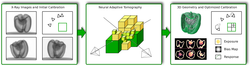
Figure 1. Neural Adaptive Tomography uses a hybrid explicit-implicit neural representation for tomographic image reconstruction. Left: The input is a set of X-ray images, typically with an ill-posed geometric configuration (sparse views or limited angular coverage). Center: NeAT represents the scene as an octree with neural features in each leaf node. This representation lends itself to an efficient differentiable rendering algorithm, presented in this paper. Right: Through neural rendering NeAT can reconstruct the 3D geometry even for ill-posed configurations, while simultaneously performing geometric and radiometric self-calibration.

NeAT: Neural Adaptive Tomography

Abstract.

In this paper, we present Neural Adaptive Tomography (NeAT), the first adaptive, hierarchical neural rendering pipeline for multi-view inverse rendering. Through a combination of neural features with an adaptive explicit representation, we achieve reconstruction times far superior to existing neural inverse rendering methods. The adaptive explicit representation improves efficiency by facilitating empty space culling and concentrating samples in complex regions, while the neural features act as a neural regularizer for the 3D reconstruction.

The NeAT framework is designed specifically for the tomographic setting, which consists only of semi-transparent volumetric scenes instead of opaque objects. In this setting, NeAT outperforms the quality of existing optimization-based tomography solvers while being substantially faster.

1. Introduction

Computed Tomography (CT) is an important scientific imaging modality in a wide range of fields, from medical imaging to material science. While most CT imaging is performed with X-rays due to their ability to penetrate a wide range of materials (Kak and Slaney, 2001), there have also been a number of works utilizing visible light, especially in the visual computing community (e.g. (Hasinoff and Kutulakos, 2007; Atcheson et al., 2008; Gregson et al., 2012; Eckert et al., 2019; Zang et al., 2020)).

The tomographic reconstruction problem is the task of estimating the 3D structure of a sample from its 2D projections. This task is well-posed under certain conditions, such as a sufficiently large number of projections/views, good angular coverage of these views, and low noise. In this situation, transform-based methods like filtered backprojection (Feldkamp et al., 1984) provide a fast and accurate reconstruction. Unfortunately, these methods no longer produce satisfactory results if the above conditions are violated (small number of views, poor angular distribution, or high noise). For these types of difficult settings, a range of iterative optimization-based methods have been developed in recent years (e.g. (Sidky and Pan, 2008; Huang et al., 2013, 2018; Zang et al., 2018a; Xu et al., 2020). These new methods greatly expand the envelope of feasible tomographic reconstruction problems, albeit at a significantly increased computational cost.

In parallel to this development, both neural rendering (e.g. (Liu et al., 2020b; Reiser et al., 2021; Garbin et al., 2021)) and differentiable rendering in general (e.g. (Nimier-David et al., 2019)) have recently garnered a lot of interest in visual computing. In particular, Neural Radiance Fields (NeRF) (Mildenhall et al., 2020), and related inverse rendering frameworks have been at the focus of attention due to their ability to provide superior reconstructions of everyday scenes with opaque objects. Similar concepts have also already been applied to the tomographic reconstruction problem (Zang et al., 2021; Sun et al., 2021). However, all the existing neural inverse rendering frameworks suffer from very long computing times. This is also true for the tomographic methods, despite operating only on 2D slice geometry, which has limited their applicability to high-resolution datasets and to the full 3D cone beam data we use in this work.

In this paper, we present Neural Adaptive Tomography (NeAT), the first adaptive, hierarchical neural rendering pipeline for multi-view inverse rendering. Through a combination of neural features with an adaptive explicit representation, we achieve reconstruction times far superior to existing neural inverse rendering methods. The adaptive explicit representation improves efficiency by facilitating empty space culling and concentrating samples in complex regions, while the neural features act as a neural regularizer for the 3D reconstruction.

NeAT is specifically tuned towards tomographic reconstruction problems, where samples are widely scattered throughout the volume, while many existing systems like NeRF (Mildenhall et al., 2020) rely on a strong concentration of samples near opaque surfaces. In this tomographic setting, we demonstrate that the purely explicit hierarchical representation of NeAT outperforms both purely implicit as well as hybrid explicit-implicit representations akin to ACORN (Martel et al., 2021) in terms of both quality and compute time. Furthermore, NeAT shows improved reconstruction quality compared to state-of-the-art tomographic reconstruction methods, while matching their performance.

In summary, the main contributions of our work are:

• An adaptive, hierarchical neural rendering pipeline based on an explicit octree representation with neural features.

• A differentiable physical sensor model for x-ray imaging that can be optimized during the reconstruction.

• An efficient open-source implementation that can be readily used on new datasets.

• An extensive evaluation of our proposed framework on different challenging tomographic reconstruction (sparse-view, limited angle, and noisy projections) of both synthetic and real data.

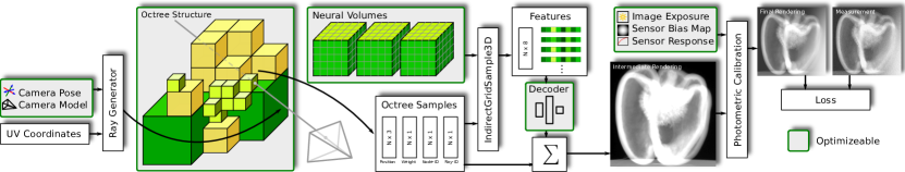
Figure 2. Overview of our adaptive neural rendering pipeline for tomographic reconstruction. To render a single pixel, we generate the corresponding ray, compute the ray-octree intersection, sample the neural volume, decode the neural features, and integrate them by a weighted sum. The estimated pixel value is then passed through a photometric calibration module resulting in the final pixel intensity. All elements in green boxes are optimized during the reconstruction. This includes the geometric and photometric calibration, the octree structure, the neural features volumes, and the neural decoder network.

2. Related Work

2.1. Classical Computed Tomography

Computed tomography is a well-established technique used for imaging the internal structures of a scanned object. It has applications in many domains, such as medicine and biology (Van Ginneken et al., 2001; Kiljunen et al., 2015; Rawson et al., 2020; Piovesan et al., 2021), material science (Brisard et al., 2020; Vásárhelyi et al., 2020), and fluid dynamics (Hasinoff and Kutulakos, 2007; Atcheson et al., 2008; Gregson et al., 2012; Eckert et al., 2019; Zang et al., 2020).

In all CT modalities, multiple projection images (sinogram) are captured from different directions. Then, reconstruction algorithms are applied to retrieve a 3D representation of the scanned object from the set of acquired projections. Several algorithm families have been deployed for tomographic reconstruction. Analytic methods based on the Radon transform and its inverse, such as filtered back projection (FBP) and its 3D cone-beam variant FDK (Feldkamp, Davis, and Kress) (Feldkamp et al., 1984), are the most used in commercial CT devices (Pan et al., 2009). These methods are fast, and accurate when a large number of uniformly sampled projections is available. However, in many situations, the number of acquired projections is low for a variety of reasons, such as the reduction of the X-ray dose (Gao et al., 2014), the deformation of the sample (Zang et al., 2018b, 2019), or its inaccessibility from some directions (Du et al., 2021a). For such scenarios, iterative reconstruction approaches have been proposed to solve a discrete formulation of the ill-posed tomography problem. The main interest of these techniques is the possibility to incorporate regularization terms like total variation in an optimization framework (Sidky and Pan, 2008; Huang et al., 2013; Kisner et al., 2012; Huang et al., 2018; Zang et al., 2018a; Xu et al., 2020; Abujbara et al., 2021). The hyper-parameter tuning and the high computational requirements are the main downsides of these approaches.

2.2. Learning-based Computed Tomography

Recently, learning-based methods have been emerging as an alternative to optimization-based reconstruction. Most of the initial proposed approaches apply neural networks either as a pre-processing or a post-processing step for traditional reconstruction methods to improve the reconstruction quality. The pre-processing networks improve the conditioning of the inverse problem by in-painting the projections (Anirudh et al., 2018; Ghani and Karl, 2018; Yoo et al., 2019; Tang et al., 2019); while the post-processing networks correct and denoise the reconstructed volume (Pelt et al., 2018; Lucas et al., 2018; Liu et al., 2020a). A third strategy consists of using a network with a differentiable forward model in order to learn a reconstruction operator (Adler and Öktem, 2018; Chen et al., 2018; Kang et al., 2018; He et al., 2020). These approaches achieve high quality results on data similar to that used for the training. They do, however, suffer from a substantial lack of generalization when applied to unseen data.

To overcome this limitation, recent studies introduce the Deep Image Prior (DIP) (Baguer et al., 2020; Barutcu et al., 2021) combined with classical regularization to constraint the reconstruction problem. On the other hand, some works proposed new approaches based on an implicit neural representation (Zang et al., 2021; Sun et al., 2021) to handle the tomography reconstruction in a self-supervised learning-based fashion. In such methods, a Multi-Layer Perceptron (MLP) network is used to represent a density field of the scanned object as a function of the input coordinates. This network is then learned from the captured projections. This representation offers an improved flexibility to generate synthetic projections at any desired resolution. This approach outperforms other existing techniques in terms of reconstruction quality. However, they are memory hungry and require a considerable learning time in the range of hours despite operating only on 2D slices based on parallel beam data. They are therefore not suitable for full 3D cone beam reconstruction. In the current paper, we propose an adaptive neural rendering framework to overcome these limitations and achieve high quality reconstructions of full 3D cone-beam data in a matter of minutes.

2.3. Implicit Neural Representations

In most tomography applications, an explicit, regular voxel grid is the representation of choice due to the simplicity of the operators. In computer graphics and computer vision, coordinate-based neural networks, also known as implicit neural representations, have recently emerged as an alternative. These consist of a neural network, typically a MLP, to learn functions that map spatial coordinates to some physical properties field (e.g. occupancy, density, color etc.). The main advantage of this representation is that the represented signal or field is implicitly defined for any given coordinate. In other words, this representation is continuous, in contrast of the discretized voxel grids. In the last two years, these coordinate-based networks have been successfully applied for modeling both static and dynamic 3D scenes and shapes (Park et al., 2019; Sitzmann et al., 2020; Martin-Brualla et al., 2021; Du et al., 2021b; Xian et al., 2021), synthesizing novel views (Eslami et al., 2018; Sitzmann et al., 2019; Mildenhall et al., 2020; Niemeyer et al., 2020; Schwarz et al., 2020; Chan et al., 2021), synthesizing texture (Oechsle et al., 2019; Saito et al., 2019; Chibane and Pons-Moll, 2020), estimating poses (Yen-Chen et al., 2020; Su et al., 2021; Wang et al., 2021), and for relighting and material editing (Boss et al., 2021; Srinivasan et al., 2021; Xiang et al., 2021; Zhang et al., 2021). In addition to a huge learning time, coordinate based networks suffer also from a slow rending speed when switching to a 3D voxel grids. Indeed, the network has to be evaluated for each single voxel, instead of querying directly a data structure.

2.4. Improving Neural Rendering

Several techniques have been proposed to speed up the volumetric rendering of coordinate-based neural networks. In Neural Sparse Voxel Fields (NSVF) approach (Liu et al., 2020b), the scene is organized into a sparse voxel octree, which is dynamically updated during the learning process. During the rendering, empty spaces are skipped, and an early rays termination are enforced. In kiloNeRF approach (Reiser et al., 2021), the standard NeRF network is factorized into a 3D grid of smaller MLPs, in order to quicken the rendering process. The AutoInt technique (Lindell et al., 2021) is based on a network that learns directly the volume integral along a ray, which makes the rendering step faster in comparison to NeRF network. FastNeRF (Garbin et al., 2021) uses caching to have a faster rendering. The standard NeRF network is split into two MLPs: a position-dependent network that generates a vector of deep radiance map, while the second network outputs the corresponding weights for a given ray direction. Yu et al. (2021) proposes a modified version of NeRF network to predict a volume density and spherical harmonic weights, which are stored in a ”PlenOctree” structure. This octree structure is then fine-tuned using a rendering loss to improve its quality. This approach allows a real-time rendering, however, the training step is still slow.

In parallel to the neural rendering approaches, researchers have also worked on simply using neural networks to represent existing images and volumes, without first solving an inverse problem. In the ACORN approach (Martel et al., 2021), the authors introduce a hybrid implicit-explicit coordinate neural representation. The learning process is accelerated through a multi-scale network architecture, which is optimized during the training in a coarse-to-fine scheme.

NeAT is somewhat inspired by all these approaches, but it is the first to solve a scene reconstruction problem by directly training a hierarchical neural representation. We show higher quality results at drastically improved training times.

3. Method

We represent the 3D scene as a sparse octree, where each leaf-node can be empty or contain a uniform grid of neural features. To query the density at a given position, the trilinear interpolated neural feature vector is passed through a small decoder network. Given a set of X-ray input images, the neural features are optimized by differentiable volume rendering. During the optimization, the octree structure is refined, and empty leaf nodes are removed from the tree. Since all steps are differentiable, we can also perform self-calibration to compute the exact camera poses, the photometric detector response and the per-image capture energy. An overview of our rendering pipeline is shown in Figure 2.

3.1. Image Formation

The raw images of digital X-ray devices represent the transmission images of a particular ray passing through an object. The image formation model in this setting derives from a continuous version of the Beer-Lambert Law (Kak and Slaney, 2001). For a given image pixel $p$, the observed pixel value is given as

(1) $$\hat{I}(p)=\hat{I}_{0}(p)\exp\left[-\int_{{t_{n}}}^{{t_{f}}}\sigma(r_{p}(t))\ dt\right],$$

where $\hat{I}_{0}$ is the (potentially spatially varying) intensity of the x-ray source, $r_{p}$ is the ray associated with the image pixel $p$, and ${t_{n}}$ and ${t_{f}}$ are the ray parameters representing the entry (near) and exit (far) point for a bounding box of the scene that represents the reconstruction region. In tomographic imaging, we seek to reconstruct the 3D distribution of $\sigma(\mathbf{x})$ (the attenuation cross section or density) within this bounding box. This reconstruction is usually performed in logarithmic space, i.e.

(2) $$\left(I_{0}(p)-I(p)\right)=\int_{{t_{n}}}^{{t_{f}}}\sigma(r_{p}(t))\ dt,$$

with $I=\log\hat{I}$ and $I_{0}=\log\hat{I}_{0}$. In this formulation, each pixel value $I(p)$ is computed as the line integral along the corresponding viewing ray $r_{p}$. The discretization of (2) converts the integral into a finite sum.

(3) $$(I_{0}(p)-I(p))\approx\sum_{i=1}^{N_{p}}\sigma(r_{p}(t_{i}))\delta_{i}.$$

Here, $N_{p}$ represents the number of samples for the particular ray, and $\delta_{i}$ denotes the length of the ray segment covered by sample $i$ (see next subsection).

3.2. Ray Sampling

Given the octree structure and a specific ray $r$, the first step in ray tracing is to generate a list of weighted samples $\{(t_{0},\delta_{0}),(t_{1},\delta_{1}),\dots\}$. This process is visualized in Figure 3 and starts by computing the ray segments $\{(n_{0},{t_{n}}_{0},{t_{f}}_{0}),(n_{1},{t_{n}}_{1},{t_{f}}_{1}),\dots\}$ that correspond to the intersection of the ray with octree node $n_{i}$. Each segment consists of the node ID as well as the scalar ray parameters ${t_{n}}_{i},{t_{f}}_{i}$ corresponding to the near and far points of the segment. We then determine how many samples should be placed along each of the segments as

(4) $$k_{i}=\Bigl{\lceil}\ N\cdot\frac{{t_{f}}_{i}-{t_{n}}_{i}}{diag(n_{i})}\ \Bigr{\rceil},$$

with $N$ being a hyper parameter that represents the maximum number of samples per node and $diag(n_{i})$ being the diagonal size of node $n_{i}$.

This approach ensures $k_{i}\in[1,N]$ and that the number of samples is proportional to the relative length of the segment but independent of node size. Small nodes obtain, on average, the same number of samples as large nodes, which in turn yields a higher sample density in subdivided regions that have been identified as regions of high geometric complexity.

Once $k_{i}$ has been determined, the interval is sampled either uniformly (during the test stage) or with stratified random sampling (during the training stage). Finally, we compute the sample weight $\delta_{j}$ as:

(5) $$\delta_{j}=\begin{cases}\frac{1}{2}(t_{0}+t_{1})-{t_{n}},&\text{if }j=0\\ {t_{f}}-\frac{1}{2}(t_{k-2}+t_{k-1}),&\text{if }j=k-1\\ \frac{1}{2}(t_{j}+t_{j+1})-\frac{1}{2}(t_{j-1}+t_{j}),&\text{else}\end{cases}$$

Note that Eq. (5) corresponds to numerical integration with central differences while related work, i.e. NeRF (Mildenhall et al., 2020), make use of forward differences only. That approach is incompatible with hierarchical adaptive sampling because empty nodes in the middle break forward integration across node boundaries.

Figure 3. Ray-sampling of the sparse octree structure. (1.) Intersection intervals of non-empty leaf nodes are computed. (2.) Samples are distributed by stratified random sampling. Note here that the intervals $({t_{n}}_{0},{t_{f}}_{0})$ and $({t_{n}}_{2},{t_{f}}_{2})$ are assigned the same $k=3$ number of samples even though the latter covers more space. (3.) The integration weight $\delta$ is computed using Eq. (5).

3.3. Tree Query

After sampling the rays, the next step is to retrieve the neural feature vector at the sample locations. To that end, we compute the global coordinate $\mathbf{x}_{g}=r(t)$ and convert it into local space of the containing leaf node. This local coordinate is then used to sample a regular grid of neural features $f_{i}$ and interpolate with trilinear weights to obtain a feature vector $f(\mathbf{x})$ for the sample location. The process is visualized in Figure 4. Note here that at the boundary between two nodes, duplicated and non-manifold features are stored in memory. A regularizer is used to resolve this issue (see Section 3.5).

Figure 4. Section of an octree structure that shows the alignment and sampling of the uniform grid inside each node. At the boundary of different nodes, some features are duplicated, and others are non-manifold.

Due to our sampling strategy (see Section 3.2), each ray and each node can have a different number of samples assigned to them. To this end, we implement an indirect 3D grid sample kernel that can compute the neural feature vector from the local coordinate and the node ID in one step. Experiments show that this custom layer is around three times more efficient than a sort-and-batch implementation using standard deep learning operators.

3.4. Decoder Network

Once the feature vector has been obtained, we transform it into the desired output domain using a global decoder network

$$\Phi:\left\{f(\mathbf{x})\right\}\rightarrow\sigma(\mathbf{x})$$

that is shared among all nodes. In the case of tomography, the output is a single scalar, representing the volume density $\sigma(\mathbf{x})$ at the sample point $\mathbf{x}$. The decoder itself is a three layer MLP with 64 neurons each, for a total of 4801 parameters to learn. We use SiLU activation functions (Elfwing et al., 2018) inside the MLP and a single SoftPlus activation after the last layer to obtain a physically meaningful positive density value. Finally, the density values are multiplied by the per-sample weight $\delta$ and summed up using a scatter-add operation resulting in the ray-integral of Eq. (3).

3.5. Loss and Regularization

We optimize the neural features and the decoder’s parameters using the mean squared error between the estimated and measured ray integrals, a total variation (TV) regularizer, and a boundary consistency (BC) regularizer.

(6) $$\mathcal{L}_{total}=\sum_{p}||I(p)-I^{\prime}(p)||^{2}+\lambda_{TV}\mathcal{L}_{TV}+\lambda_{BC}\mathcal{L}_{BC},$$

where $I^{\prime}(p)$ is the estimated ray integral for ray $r_{p}$, $I(p)$ the measured image intensity, and $\lambda_{TV},\lambda_{BC}$ are hyper parameters that control the strength of each regularizer.

The TV loss acts as an additional spatial regularized during the training, and has a similar role to the TV loss used in optimization-based methods. To compute the TV loss, we utilize the regular structure of the feature grids $f_{n}$ for each node. The loss can either be computed directly on the feature vectors, or on the decoded densities:

(7) $$\mathcal{L}_{TV}^{(1)}=\sum_{n}\|\nabla f_{n}\|_{1}\quad\quad\text{or}\quad\quad\mathcal{L}_{TV}^{(2)}=\sum_{n}\|\nabla\Phi(f_{n})\|_{1}.$$

We experimented both variants and found that the former variant produces slightly better results in addition to being faster.

The boundary consistency regularizer ensures a smooth transition between two neighboring nodes. This is important, because as described in Section 3.3, duplicated and non-manifold features are stored along the node boundary. This will result in block-like artifacts especially if only few images are used. The regularizer minimizes the feature error on the boundary surface $\Lambda_{nm}$ for two neighboring octree nodes $n$ and $m$

(8) $$\mathcal{L}_{BC}=\sum_{(n,m)\in\mathcal{N}}\ \sum_{x\in\Lambda_{nm}}|f_{m}(x)-f_{n}(x)|,$$

where $\mathcal{N}$ denotes the set of all pairs of neighboring nodes.

3.6. Self-Calibration

CT reconstruction of real data often requires several calibration steps both regarding the camera geometry and the radiometric properties.

Radiometric self-calibration.

As can be seen in Eq. (2), tomographic reconstruction requires a reference image $I_{0}$ representing the illumination pattern without an object present. In cone-beam CT, this image captures effects such as the intensity dropoff towards the image boundaries due to the cosine and $1/r^{2}$ terms, as well as any other non-uniformities in the illumination. Unfortunately, adding or removing the object from the setup can also disturb the validity the reference image, causing artifacts in the reconstruction. The differentiable nature of the NeAT framework allows us to refine (or estimate from scratch) the reference image $I_{0}$, as well as a per-view multiplier representing potentially different exposure times for each view. Variations in exposure time are appropriate if the object is much thicker in one direction than in another. Optimizing these parameters can significantly improve the reconstruction quality, depending on the dataset.

Geometric self-calibration.

High resolution tomographic reconstruction also relies on the availability of high precision camera extrinsics and intrinsics. Although in cone-beam CT the camera pose is usually controlled with a high precision turntable, parameters such as the precise field-of-view or the exact location of the rotation axis in the image plane can be much harder to calibrate accurately, and in fact they may drift over time due to heat expansion and other factors. We instead propose to only use approximate parameter estimation to get the camera model into the right ballpark, and to then rely on gradient backpropagation to update the camera parameters, including the relative positioning of the source and detector, as well as the exact rotation angles between the views.

3.7. Octree Update

To automatically update the octree structure during the reconstruction, we loosely follow the method of ACORN (Martel et al., 2021). However, while ACORN has access to a ground truth image/volume data at every point in the cell, this ground truth is not available in tomographic reconstruction tasks where the only error metric available is the 2D reprojection error in each of the views.

From this 2D image space error we estimate a volumetric error distribution by summing over all the reprojection errors for ray intersecting a given node. I.e. for a specific node $n$, the node error becomes

(9) $$E(n)=\sigma_{\max}(n)\cdot\sum_{(p,t,\delta)\in\Omega_{n}}\delta||I(p)-\tilde{I}(p)||^{2},$$

where $\Omega_{n}$ refers to the set of all samples $(t,\delta)$ in $n$ from any ray passing through the node $n$, paired with the pixel coordinates $p$ that generated the ray. $\tilde{I}$ refers to the reprojection of the current volume estimate. The summation term therefore corresponds to a coarse tomographic reconstruction of the reprojection error, integrated over the octree node. This volumetric measure of error is additionally weighted by the maximum density of the node, $\sigma_{\max}(n)=\max_{(t,\delta)\in\Omega_{n}}\sigma(r(t))$.

Using this per-node error we then solve a mixed-integer program (MIP), which finds the best tree configuration with respect to a real-valued objective function. Linear constraints ensure that at most $T_{max}$ leaf nodes are used and the configuration is a valid octree. The details can be found in (Martel et al., 2021) as well as in our source code.

4. Experiments

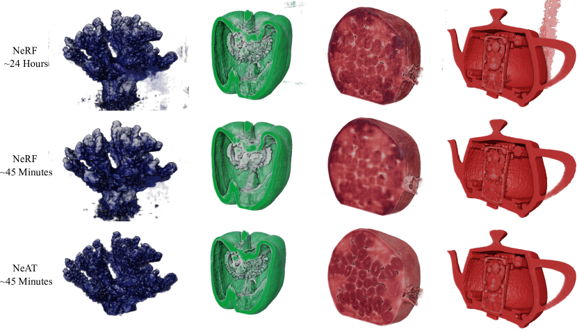
Figure 5. 3D volume renderings of the real datasets, as reconstructed by NeRF and NeAT using 25-50 projections. From left to right: ceramic coral, pepper, pomegranate, wind-up teapot. See Figure 12 for a 2D slice comparison.

4.1. Datasets and Evaluation Metric

In the following, we present several reconstruction experiments on various CT datasets. We divide these datasets into two classes: Real Data and Synthetic Data. The real datasets are captured using a Nikon industrial CT scanner. These images are noisy and some geometric and radiometric calibration errors are expected. Since we don’t have a ground-truth volume of the real datasets, we evaluate the performance using the reprojection error. In particular, the scanner provides us with a set of real X-ray images, which we split into a training and test set. The training set is used to reconstruct the volume and the test set is used for the evaluation. Figure 5 shows 3D renderings of NeAT reconstructions for all real datasets.

The synthetic datasets are given in the form of a volume sampled on a regular voxel grid, which we use to generate synthetic X-ray images from different angles. By construction, there is no calibration error or image noise in the rendered views, however we add some synthetic Gaussian noise back in. To evaluate the reconstruction quality of synthetic datasets, we can directly compare the estimated volume towards the ground-truth volume, although the reprojection error can also be useful to assess overfitting.

4.2. Ablation Studies

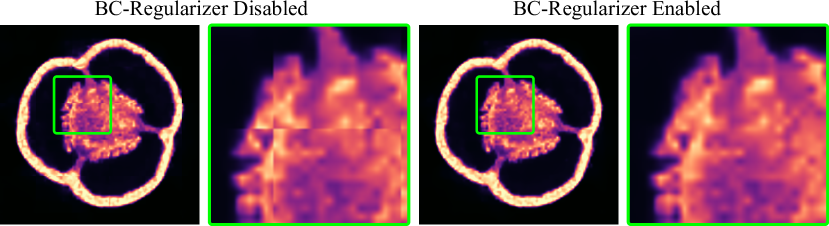
Figure 6. Sparse view tomography on the Pepper dataset with and without boundary consistency (BC) regularizer. Sharp edges at the boundary between neighboring octree nodes are successfully removed.

	Sparse View			Limitted Angle
$\lambda_{TV}$	Train $\uparrow$	Test $\uparrow$	Vol. $\uparrow$	Train $\uparrow$	Test $\uparrow$	Vol. $\uparrow$
0.00000	43.97	38.58	34.41	48.07	26.37	22.20
0.00002	43.21	39.32	35.96	46.74	27.1	22.81
0.00010	41.74	39.17	35.25	44.95	27.92	23.56
0.00025	40.69	38.63	34.67	43.50	27.36	23.38
0.00050	39.44	37.47	33.10	42.67	26.89	23.02

Table 1. Reprojection error (PSNR) of the training and test views, as well as volumetric PSNR on the pepper dataset for different values of TV regularization.

Regularziation

To regularize the reconstruction, we have implemented the TV- and BC-regularizer (see Section 3.5). The BC-regularizer (Eq. 8) ensures a smooth transition between neighboring octree nodes. This is demonstrated in Figure 6, which shows block-like artifacts if BC is disabled. We found that $\lambda_{BC}=0.01$ gives good result on all datasets and is therefore used in the further experiments. The TV-regularizer (Eq. 7) is used to further constrain underdetermined reconstruction problems, i.e., sparse view and limited angle tomography. Table 1 shows both the reprojection errors on training views as well as on previously unseen test views. In addition we show the volume error directly. The training and test reprojection errors demonstrate that overfitting can be reduced by increasing $\lambda_{TV}$. This also improves the volumetric error. We found that for sparse view problems $\lambda_{TV}=0.00002$ and for limited angle problems $\lambda_{TV}=0.00010$ gives the best results.

Geometric Self-Calibration

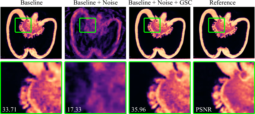
Figure 7. Ablation study of geometric self calibration on real data. Baseline (left column) is the reconstruction using the initial calibration provided by the CT scanner. Adding noise to that calibration significantly degrades the result (second column). Our geometric self-calibration (GSC) can recover from the noisy input and even outperform the baseline calibration slightly (third column).

As described in Section 3.6 our system can optimize the geometric parameters, such as detector orientation and source position, during the reconstruction. In Figure 7, we show the difference on a real dataset with geometric self-calibration enabled and disabled. On the left, the baseline experiment is presented using the geometry configuration from the CT scanner. Then we add Gaussian noise to the position and rotation of each view. This degrades the reconstruction by 15 dB. Using our geometric self calibration (GSC) our pipeline recovers from this bad initial calibration and then even outperform the baseline setting. It is therefore robust and improves the reconstruction of real CT data.

Radiometric Self-Calibration

Figure 8. Sparse view tomography on the pepper dataset with and without radiometric self calibration. The bottom row shows the same volume multiplied by four to highlight noisy empty regions.

To test the effectiveness of radiometric self-calibration, we run our reconstruction pipeline on the real datasets and disables individual steps. The results are presented in Figure 8. The first experiment is the baseline with radiometric self calibration disabled. After that we enable exposure and sensor bias estimation which improves the reconstruction by around 1 dB. Enabling the response curve optimization, further improves the result, which can be seen in the amplified image at the bottom.

Decoder

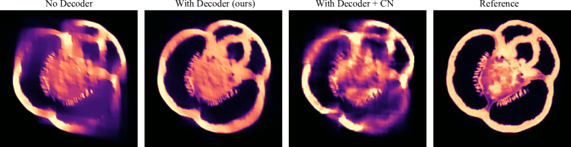
Figure 9. Limited angle reconstruction without decoder, with decoder, and with decoder and ACORN-style coordinate network (CN).

Next, we want to analyze the usefulness of the decoder network with respect to reconstruction quality and regularization properties. In our current implementation, we use an eight-element feature vector which is transformed into a single density value by the decoder network. The counterpart is a pipeline without decoder but double resolution blocks in x,y,z direction. The volume has then exactly the same amount of variables but without the feature decoder. Figure 9 shows the result of this comparison on a limited angle problem. On the left hand side, we have the no-decoder variant with a grid resolution of $1\times 33^{3}$. On the right, our full pipeline is displayed, which uses a grid resolution of $8\times 17^{3}$. Using the decoder network, the sides of the fruit are reconstructed more accurately. Without it, blurry artifacts appear, which are similar to artifacts of the iterative reconstructions methods. We can therefore infer a regularizing property of the decoder network that improves the reconstruction in difficult conditions.

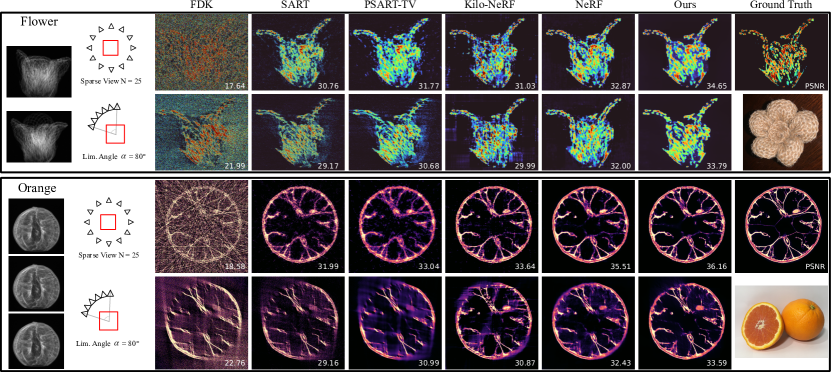
Figure 10. Sparse view and limited angle reconstructions on synthetic CT datasets. In the left most column, some raw input images are shown together with the reconstruction configuration. In the right most column, we show the Ground Truth, and illustrating images of the scanned objects. This comparison shows that our method (Ours) outperforms other baseline methods both qualitatively and quantitatively.

Explicit vs. Hybrid explicit-implicit representation.

The neural feature volumes in our reconstruction pipeline is stored explicitly as a large tensor (see Figure 2). An alternative design would be a hybrid explicit-implicit model, like ACORN (Martel et al., 2021) in which the feature volumes are not stored explicitly, but are further compressed into an implicit neural network in the hope of achieving additional compression and regularization. Unfortunately, this hope does not materialize in the context of tomographic reconstruction (Figure 9, third sub-image). Specifically, we found that the PSNR for hybrid explicit-implicit representations are worse than for our purely explicit hierarchical representation, especially in the case of limited angle tomography. In limited angle tomography, reconstructions are already blurred in the direction orthogonal to the missing viewing direction (missing wedge problem). The additional regularization of the implicit network further encourages this blur instead of repairing it.

Moreover, adding an implicit network dramatically increases the training times. Finally, while final explicit-implicit representation is more compact than our explicit one, the intermediate memory consumption during training is actually higher, since all feature volumes need to be decoded in order to trace all rays for one view.

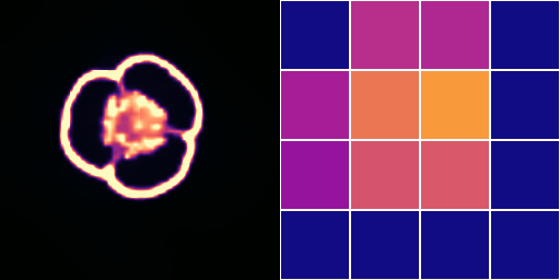
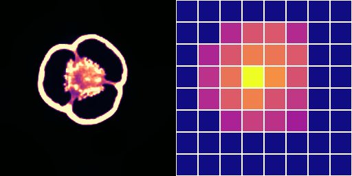
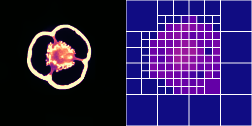
Figure 11. Adaptive reconstruction of the pepper dataset. At the right side of each slice the octree structure is visualized. The color indicate the per-node error as defined in Eq. (9). This error is used to optimally distribute a fixed number of leaf nodes onto the scene. The bottom right shows the training loss during the reconstruction. The tree structure is optimized once a convergence has been detected, here at step 2200 and 5400.

Structure Refinement

In Section 3.7, we describe the structural octree optimization, which is performed every few epochs during the reconstruction. This optimization consists of merging, splitting, and culling leaf nodes from the tree. From these transformations, we expect a shorter reconstruction time, due to empty space skipping, and a more accurate reconstruction, due to allocating more resources to difficult parts of the scene. The structure optimization process is presented in Figure 11 on the pepper dataset with a maximum number of 1024 leaf nodes. The octree is initialized by a uniform grid of resolution $4^{3}=64$. Once the training has converged on that resolution the per-node error is computed using Eq. (9) and the structure refinement is applied. From top left to top right all leaf nodes are split because a full split doesn’t exceed the leaf node budged $8^{3}=512<1024$. However, at the next structure refinement step, splitting all nodes again is not possible $16^{3}=4096>1024$. The optimization therefore automatically merges low-error nodes to split more high-error leaves. Note that in this example, the empty space culling has been disabled to demonstrate adaptive node allocation. The graph in the bottom left of Figure 11 shows the loss curve during the reconstruction. The steep steps indicate the points of structure optimization.

4.3. Comparison to Existing Methods

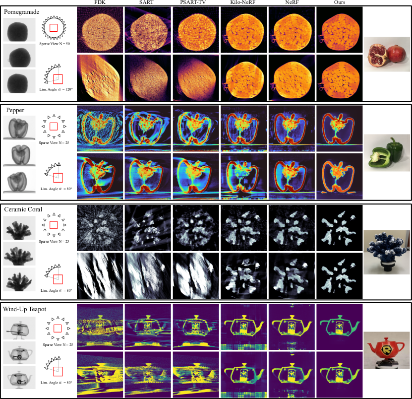
Figure 12. Sparse view and limited angle reconstructions on real CT datasets. In the left most column, some raw input images are shown together with the reconstruction configuration. In the right most column, we show illustrating images of the scanned objects. This comparison show that our method (Ours) achieves high-quality results for all data and for the two configurations.

We have evaluated our CT reconstruction method on various datasets and compare it to other state-of-the-art approaches. The other methods are cone-beam filtered backprojection (FDK) (Feldkamp et al., 1984), the Simultaneous Algebraic Reconstruction (SART)(Kak and Slaney, 2001), the proximal SART with TV regularizer (PSART-TV) (Zang et al., 2018a), The Neural Radiance Fields (NeRF)  (Mildenhall et al., 2020)), and a NeRF variant making use of separate local implicit functions (Kilo-NeRF) (Reiser et al., 2021). The first three are traditional CT-reconstruction approaches and variants of these are usually found in commercial CT systems. The latter two are modern rendering approaches originally designed for novel view synthesis and multi-view reconstruction. We have adapted them to handle X-ray input data by changing the compositing operator to our image formation model. Furthermore, we modified Kilo-NeRF by disabling the student-teacher distilling to validate if a direct training of local MLPs is possible.

The algebraic reconstruction techniques are run until convergence which takes between 5-30 minutes for simple methods like SART, according to the number of projections used, but takes about 40-50 minutes on for more advanced methods like PSART-TV. For the optimization-based methods, we conduct a parameter search and present the best quality results. NeRF and Kilo-Nerf are trained for 24h and our approach is run for 40 epochs corresponding to around 45 minutes on an A100 GPU. When comparing the times, it is important to keep in mind the vastly different code bases, and the fact that all methods have a significant number of parameters and hyper parameters that affect the timing. The provided times are therefore only to be interpreted as rough indicators of compute performance. Please also see the discussion in Section 5.

In the first experiments, we measure the reconstruction quality on synthetic data. The volume is known a priori and the projection images are generated by volume rendering. On each projection, we add Gaussian noise with a standard deviation of $\sigma=0.02\cdot I_{max}$. No other calibrations errors are simulated. The resulting reconstructions of each method are presented in Figure 10. The first two rows depict sparse-view and limited angle tomography on the flower dataset. The same is done for the Orange dataset in the following rows. All methods (except FDK) achieve decent results on both datasets and configurations. However, on the Flower dataset our method is the clear favorite with a PSNR improvement of almost 2dB over the second best. On the Orange dataset, both NeRF and Neat show a high quality reconstruction. Quantitatively our method has the edge due to its sharpness but in the limited angle reconstruction (last row), NeRF is able to complete the orange’s skin better.

After the synthetic experiment, we evaluate the same systems on four real datasets captured by a commercial CT scanner. These datasets are Pomegranate, Pepper, Ceramic Coral, and Wind-Up Teapot. They cover a wide range of interesting aspects such as the low-contrast internal structure of the pomegranate and the sophisticated mechanics of the wind-up teapot. Sample raw-images of each object are shown in Figure 12 on the left. Next to that, the current reconstruction configuration is visualized. On all four datasets and two configurations, NeAT provides the visually best reconstructions. The volume is almost noise-free, edges are sharp and fine details such as the pepper seeds are preserved. There are a few artifacts in the limited angle reconstruction, however the artifacts and noise of the other approaches are more severe.

5. Discussion and Conclusions

5.1. Discussion

In the previous section we have compared NeAT to other CT reconstruction approaches. We have shown that our approach achieves significantly improved results than baseline methods both on synthetic and real datasets. We believe that the reasoning is multilateral. First of all, we use a neural regularizer in the form of a decoder network that is able to steer the reconstruction to a physically plausible solution. Secondly, our geometric and photometric self calibration eliminates tiny errors of real-world data. Lastly, the adaptive octree refinement ensures a smart distribution of memory and computational resources to complex parts of the scene.

In terms of compute times, NeAT is comparable in compute time with advanced optimization-based methods like PSART-TV, although precise comparisons of compute time of course depend on the hyper parameters of either method, as well as the degree of code optimization.

Most of the computational effort of NeAT is spent on evaluating the decoder network, while the ray-tracing itself is substantially faster than the PSART-TV implementation. This is primarily due to two factors: our adaptive, octree-based approach that can efficiently allocate samples to interesting volume regions, and our effective use of GPUs as opposed to (already highly optimized) multicore CPU code in the reference implementations of the optimization-based approaches.

It is therefore likely that a careful GPU implementation of a hierarchical version of, for example, PSART-TV could realize similar performance gains as NeAT. However, doing so would be significantly more difficult than for NeAT: iterative solvers are based on a volume projection operator $\mathbf{A}$ and the corresponding backprojection operator $\mathbf{A}^{T}$. Since the matrices are far too large to store, $\mathbf{A}$ and $\mathbf{A}^{T}$ are implemented procedurally as separate operators, where $\mathbf{A}$ is a gather operator while $\mathbf{A}^{T}$ is a scatter operator. Even with CPU code on a uniform grid it is not trivial to get the two operators to perform well while maintaining an exact transpose relationship to each other, which is a condition for the convergence and correctness of most solvers. GPU implementations with hierarchical data structures would dramatically complicate this task further.

This is where the differentiable rendering approach of NeAT shines: instead of having to implement both operators, we only need to implement the forward operator $\mathbf{A}$ in a differentiable fashion, and can then rely on backpropagation for the optimization. By using an appropriate environment such as the PyTorch backend, the effort to implement this efficiently on a GPU is much reduced.

5.2. Limitations and Future Work

Despite these advantages, during our experiments we also found some limitations that should be worked on in the future. One general problem in adopting neural networks for scientific applications is that artifacts of traditional approaches are usually easy to spot for a human since they come in the form of strong blurriness or long streaks. In the case of neural adaptive tomography, the artifacts look physically plausible and are therefore harder to distinguish from a correct reconstruction. For example, in the teapot dataset (Figure 12 bottom), all limited angle reconstructions exhibit a topology change in the lower right corner. For the optimization-based methods it is obvious that these regions cannot be trusted, whereas the deep learning methods show plausible low-frequency completions of the geometry, which however do not match reality.

As a further limitation, we also note that our method is currently only suitable for a tomographic image formation model, which can be evaluated in an order-independent fashion (2). Reconstructions of opaque objects require a compositing image formation model similar to NeRF (Mildenhall et al., 2020), which requires all volume samples to be ordered front to back. With our hierarchical octree subdivision of space this would require additional book keeping efforts. Furthermore, we believe the sampling strategy would likely have to be adapted for this type of scene to concentrate the samples close to object surfaces.

5.3. Conclusion

In summary, we have presented NeAT, the first neural rendering architecture to directly train an adaptive, hierarchical neural representation from images. This approach yields superior image quality and training time compared to other recent neural rendering methods. Compared to traditional optimization-based tomography solvers, NeAT shows better quality while matching the computational performance.

While NeAT is at the moment optimized for tomographic reconstruction, we believe that similar concepts can be employed to reconstruct complex scenes with opaque surfaces. This, however, we leave for future work.

- (1)
- Abujbara et al. (2021) Khaled Abujbara, Ramzi Idoughi, and Wolfgang Heidrich. 2021. Non-Linear Anisotropic Diffusion for Memory-Efficient Computed Tomography Super-Resolution Reconstruction. In 2021 International Conference on 3D Vision (3DV). IEEE, 175–185.
- Adler and Öktem (2018) Jonas Adler and Ozan Öktem. 2018. Learned primal-dual reconstruction. IEEE transactions on medical imaging 37, 6 (2018), 1322–1332.
- Anirudh et al. (2018) Rushil Anirudh, Hyojin Kim, Jayaraman J Thiagarajan, K Aditya Mohan, Kyle Champley, and Timo Bremer. 2018. Lose the views: Limited angle CT reconstruction via implicit sinogram completion. In Proceedings of the IEEE Conference on Computer Vision and Pattern Recognition. 6343–6352.
- Atcheson et al. (2008) Bradley Atcheson, Ivo Ihrke, Wolfgang Heidrich, Art Tevs, Derek Bradley, Marcus Magnor, and Hans-Peter Seidel. 2008. Time-resolved 3d capture of non-stationary gas flows. ACM transactions on graphics (TOG) 27, 5 (2008), 1–9.
- Baguer et al. (2020) Daniel Otero Baguer, Johannes Leuschner, and Maximilian Schmidt. 2020. Computed tomography reconstruction using deep image prior and learned reconstruction methods. Inverse Problems 36, 9 (2020), 094004.
- Barutcu et al. (2021) Semih Barutcu, Selin Aslan, Aggelos K Katsaggelos, and Doğa Gürsoy. 2021. Limited-angle computed tomography with deep image and physics priors. Scientific reports 11, 1 (2021), 1–12.
- Boss et al. (2021) Mark Boss, Raphael Braun, Varun Jampani, Jonathan T Barron, Ce Liu, and Hendrik Lensch. 2021. Nerd: Neural reflectance decomposition from image collections. In Proceedings of the IEEE/CVF International Conference on Computer Vision. 12684–12694.
- Brisard et al. (2020) Sébastien Brisard, Marijana Serdar, and Paulo JM Monteiro. 2020. Multiscale X-ray tomography of cementitious materials: A review. Cement and Concrete Research 128 (2020), 105824.
- Chan et al. (2021) Eric R Chan, Marco Monteiro, Petr Kellnhofer, Jiajun Wu, and Gordon Wetzstein. 2021. pi-gan: Periodic implicit generative adversarial networks for 3d-aware image synthesis. In Proceedings of the IEEE/CVF Conference on Computer Vision and Pattern Recognition. 5799–5809.
- Chen et al. (2018) Hu Chen, Yi Zhang, Yunjin Chen, Junfeng Zhang, Weihua Zhang, Huaiqiang Sun, Yang Lv, Peixi Liao, Jiliu Zhou, and Ge Wang. 2018. LEARN: Learned experts’ assessment-based reconstruction network for sparse-data CT. IEEE transactions on medical imaging 37, 6 (2018), 1333–1347.
- Chibane and Pons-Moll (2020) Julian Chibane and Gerard Pons-Moll. 2020. Implicit feature networks for texture completion from partial 3d data. In European Conference on Computer Vision. Springer, 717–725.
- Du et al. (2021a) Jianguo Du, Guangming Zang, Balaji Mohan, Ramzi Idoughi, Jaeheon Sim, Tiegang Fang, Peter Wonka, Wolfgang Heidrich, and William L Roberts. 2021a. Study of spray structure from non-flash to flash boiling conditions with space-time tomography. Proceedings of the Combustion Institute 38, 2 (2021), 3223–3231.
- Du et al. (2021b) Yilun Du, Yinan Zhang, Hong-Xing Yu, Joshua B Tenenbaum, and Jiajun Wu. 2021b. Neural radiance flow for 4d view synthesis and video processing. In Proceedings of the IEEE/CVF International Conference on Computer Vision. 14324–14334.
- Eckert et al. (2019) Marie-Lena Eckert, Kiwon Um, and Nils Thuerey. 2019. ScalarFlow: a large-scale volumetric data set of real-world scalar transport flows for computer animation and machine learning. ACM Transactions on Graphics (TOG) 38, 6 (2019), 1–16.
- Elfwing et al. (2018) Stefan Elfwing, Eiji Uchibe, and Kenji Doya. 2018. Sigmoid-weighted linear units for neural network function approximation in reinforcement learning. Neural Networks 107 (2018), 3–11.
- Eslami et al. (2018) SM Ali Eslami, Danilo Jimenez Rezende, Frederic Besse, Fabio Viola, Ari S Morcos, Marta Garnelo, Avraham Ruderman, Andrei A Rusu, Ivo Danihelka, Karol Gregor, et al. 2018. Neural scene representation and rendering. Science 360, 6394 (2018), 1204–1210.
- Feldkamp et al. (1984) Lee A Feldkamp, Lloyd C Davis, and James W Kress. 1984. Practical cone-beam algorithm. Josa a 1, 6 (1984), 612–619.
- Gao et al. (2014) Yang Gao, Zhaoying Bian, Jing Huang, Yunwan Zhang, Shanzhou Niu, Qianjin Feng, Wufan Chen, Zhengrong Liang, and Jianhua Ma. 2014. Low-dose X-ray computed tomography image reconstruction with a combined low-mAs and sparse-view protocol. Optics express 22, 12 (2014), 15190–15210.
- Garbin et al. (2021) Stephan J Garbin, Marek Kowalski, Matthew Johnson, Jamie Shotton, and Julien Valentin. 2021. FastNeRF: High-fidelity neural rendering at 200fps. arXiv preprint arXiv:2103.10380 (2021).
- Ghani and Karl (2018) Muhammad Usman Ghani and W Clem Karl. 2018. Deep learning-based sinogram completion for low-dose CT. In 2018 IEEE 13th Image, Video, and Multidimensional Signal Processing Workshop (IVMSP). IEEE, 1–5.
- Gregson et al. (2012) James Gregson, Michael Krimerman, Matthias B Hullin, and Wolfgang Heidrich. 2012. Stochastic tomography and its applications in 3D imaging of mixing fluids. 31, 4 (2012), 52–1.
- Hasinoff and Kutulakos (2007) Samuel W Hasinoff and Kiriakos N Kutulakos. 2007. Photo-consistent reconstruction of semitransparent scenes by density-sheet decomposition. 29, 5 (2007), 870–885.
- He et al. (2020) Ji He, Yongbo Wang, and Jianhua Ma. 2020. Radon inversion via deep learning. IEEE transactions on medical imaging 39, 6 (2020), 2076–2087.
- Huang et al. (2013) Jing Huang, Yunwan Zhang, Jianhua Ma, Dong Zeng, Zhaoying Bian, Shanzhou Niu, Qianjin Feng, Zhengrong Liang, and Wufan Chen. 2013. Iterative image reconstruction for sparse-view CT using normal-dose image induced total variation prior. PloS one 8, 11 (2013), e79709.
- Huang et al. (2018) Yixing Huang, Oliver Taubmann, Xiaolin Huang, Viktor Haase, Guenter Lauritsch, and Andreas Maier. 2018. Scale-space anisotropic total variation for limited angle tomography. IEEE Transactions on Radiation and Plasma Medical Sciences 2, 4 (2018), 307–314.
- Kak and Slaney (2001) Avinash C Kak and Malcolm Slaney. 2001. Principles of computerized tomographic imaging. SIAM.
- Kang et al. (2018) Eunhee Kang, Won Chang, Jaejun Yoo, and Jong Chul Ye. 2018. Deep convolutional framelet denosing for low-dose CT via wavelet residual network. IEEE transactions on medical imaging 37, 6 (2018), 1358–1369.
- Kiljunen et al. (2015) Timo Kiljunen, Touko Kaasalainen, Anni Suomalainen, and Mika Kortesniemi. 2015. Dental cone beam CT: A review. Physica Medica 31, 8 (2015), 844–860.
- Kisner et al. (2012) Sherman J Kisner, Eri Haneda, Charles A Bouman, Sondre Skatter, Mikhail Kourinny, and Simon Bedford. 2012. Model-based CT reconstruction from sparse views. In Second International Conference on Image Formation in X-Ray Computed Tomography. 444–447.
- Lindell et al. (2021) David B Lindell, Julien NP Martel, and Gordon Wetzstein. 2021. Autoint: Automatic integration for fast neural volume rendering. In Proceedings of the IEEE/CVF Conference on Computer Vision and Pattern Recognition. 14556–14565.
- Liu et al. (2020b) Lingjie Liu, Jiatao Gu, Kyaw Zaw Lin, Tat-Seng Chua, and Christian Theobalt. 2020b. Neural sparse voxel fields. arXiv preprint arXiv:2007.11571 (2020).
- Liu et al. (2020a) Zhengchun Liu, Tekin Bicer, Rajkumar Kettimuthu, Doga Gursoy, Francesco De Carlo, and Ian Foster. 2020a. TomoGAN: low-dose synchrotron x-ray tomography with generative adversarial networks: discussion. JOSA A 37, 3 (2020), 422–434.
- Lucas et al. (2018) Alice Lucas, Michael Iliadis, Rafael Molina, and Aggelos K Katsaggelos. 2018. Using deep neural networks for inverse problems in imaging: beyond analytical methods. IEEE Signal Processing Magazine 35, 1 (2018), 20–36.
- Martel et al. (2021) Julien NP Martel, David B Lindell, Connor Z Lin, Eric R Chan, Marco Monteiro, and Gordon Wetzstein. 2021. ACORN: Adaptive Coordinate Networks for Neural Scene Representation. arXiv preprint arXiv:2105.02788 (2021).
- Martin-Brualla et al. (2021) Ricardo Martin-Brualla, Noha Radwan, Mehdi SM Sajjadi, Jonathan T Barron, Alexey Dosovitskiy, and Daniel Duckworth. 2021. Nerf in the wild: Neural radiance fields for unconstrained photo collections. In Proceedings of the IEEE/CVF Conference on Computer Vision and Pattern Recognition. 7210–7219.
- Mildenhall et al. (2020) Ben Mildenhall, Pratul P Srinivasan, Matthew Tancik, Jonathan T Barron, Ravi Ramamoorthi, and Ren Ng. 2020. Nerf: Representing scenes as neural radiance fields for view synthesis. In European conference on computer vision. Springer, 405–421.
- Niemeyer et al. (2020) Michael Niemeyer, Lars Mescheder, Michael Oechsle, and Andreas Geiger. 2020. Differentiable volumetric rendering: Learning implicit 3d representations without 3d supervision. In Proceedings of the IEEE/CVF Conference on Computer Vision and Pattern Recognition. 3504–3515.
- Nimier-David et al. (2019) Merlin Nimier-David, Delio Vicini, Tizian Zeltner, and Wenzel Jakob. 2019. Mitsuba 2: A retargetable forward and inverse renderer. ACM Transactions on Graphics (TOG) 38, 6 (2019), 1–17.
- Oechsle et al. (2019) Michael Oechsle, Lars Mescheder, Michael Niemeyer, Thilo Strauss, and Andreas Geiger. 2019. Texture fields: Learning texture representations in function space. In Proceedings of the IEEE/CVF International Conference on Computer Vision. 4531–4540.
- Pan et al. (2009) Xiaochuan Pan, Emil Y Sidky, and Michael Vannier. 2009. Why do commercial CT scanners still employ traditional, filtered back-projection for image reconstruction? Inverse problems 25, 12 (2009), 123009.
- Park et al. (2019) Jeong Joon Park, Peter Florence, Julian Straub, Richard Newcombe, and Steven Lovegrove. 2019. Deepsdf: Learning continuous signed distance functions for shape representation. In Proceedings of the IEEE/CVF Conference on Computer Vision and Pattern Recognition. 165–174.
- Pelt et al. (2018) Daniël M Pelt, Kees Joost Batenburg, and James A Sethian. 2018. Improving tomographic reconstruction from limited data using mixed-scale dense convolutional neural networks. Journal of Imaging 4, 11 (2018), 128.
- Piovesan et al. (2021) Agnese Piovesan, Valérie Vancauwenberghe, Tim Van De Looverbosch, Pieter Verboven, and Bart Nicolaï. 2021. X-ray computed tomography for 3D plant imaging. Trends in Plant Science 26, 11 (2021), 1171–1185.
- Rawson et al. (2020) Shelley D Rawson, Jekaterina Maksimcuka, Philip J Withers, and Sarah H Cartmell. 2020. X-ray computed tomography in life sciences. BMC biology 18, 1 (2020), 1–15.
- Reiser et al. (2021) Christian Reiser, Songyou Peng, Yiyi Liao, and Andreas Geiger. 2021. KiloNeRF: Speeding up Neural Radiance Fields with Thousands of Tiny MLPs. arXiv preprint arXiv:2103.13744 (2021).
- Saito et al. (2019) Shunsuke Saito, Zeng Huang, Ryota Natsume, Shigeo Morishima, Angjoo Kanazawa, and Hao Li. 2019. Pifu: Pixel-aligned implicit function for high-resolution clothed human digitization. In Proceedings of the IEEE/CVF International Conference on Computer Vision. 2304–2314.
- Schwarz et al. (2020) Katja Schwarz, Yiyi Liao, Michael Niemeyer, and Andreas Geiger. 2020. Graf: Generative radiance fields for 3d-aware image synthesis. arXiv preprint arXiv:2007.02442 (2020).
- Sidky and Pan (2008) Emil Y Sidky and Xiaochuan Pan. 2008. Image reconstruction in circular cone-beam computed tomography by constrained, total-variation minimization. Physics in Medicine & Biology 53, 17 (2008), 4777.
- Sitzmann et al. (2020) Vincent Sitzmann, Julien NP Martel, Alexander W Bergman, David B Lindell, and Gordon Wetzstein. 2020. Implicit neural representations with periodic activation functions. arXiv preprint arXiv:2006.09661 (2020).
- Sitzmann et al. (2019) Vincent Sitzmann, Michael Zollhöfer, and Gordon Wetzstein. 2019. Scene representation networks: Continuous 3d-structure-aware neural scene representations. arXiv preprint arXiv:1906.01618 (2019).
- Srinivasan et al. (2021) Pratul P Srinivasan, Boyang Deng, Xiuming Zhang, Matthew Tancik, Ben Mildenhall, and Jonathan T Barron. 2021. NeRV: Neural reflectance and visibility fields for relighting and view synthesis. In Proceedings of the IEEE/CVF Conference on Computer Vision and Pattern Recognition. 7495–7504.
- Su et al. (2021) Shih-Yang Su, Frank Yu, Michael Zollhoefer, and Helge Rhodin. 2021. A-NeRF: Surface-free Human 3D Pose Refinement via Neural Rendering. arXiv preprint arXiv:2102.06199 (2021).
- Sun et al. (2021) Yu Sun, Jiaming Liu, Mingyang Xie, Brendt Wohlberg, and Ulugbek S Kamilov. 2021. Coil: Coordinate-based internal learning for tomographic imaging. IEEE Transactions on Computational Imaging (2021).
- Tang et al. (2019) Chao Tang, Wenkun Zhang, Ziheng Li, Ailong Cai, Linyuan Wang, Lei Li, Ningning Liang, and Bin Yan. 2019. Projection super-resolution based on convolutional neural network for computed tomography. In 15th International Meeting on Fully Three-Dimensional Image Reconstruction in Radiology and Nuclear Medicine, Vol. 11072. International Society for Optics and Photonics, 1107233.
- Van Ginneken et al. (2001) Bram Van Ginneken, BM Ter Haar Romeny, and Max A Viergever. 2001. Computer-aided diagnosis in chest radiography: a survey. IEEE Transactions on medical imaging 20, 12 (2001), 1228–1241.
- Vásárhelyi et al. (2020) Lívia Vásárhelyi, Zoltán Kónya, Ákos Kukovecz, and Róbert Vajtai. 2020. Microcomputed tomography–based characterization of advanced materials: a review. Materials Today Advances 8 (2020), 100084.
- Wang et al. (2021) Zirui Wang, Shangzhe Wu, Weidi Xie, Min Chen, and Victor Adrian Prisacariu. 2021. NeRF–: Neural Radiance Fields Without Known Camera Parameters. arXiv preprint arXiv:2102.07064 (2021).
- Xian et al. (2021) Wenqi Xian, Jia-Bin Huang, Johannes Kopf, and Changil Kim. 2021. Space-time neural irradiance fields for free-viewpoint video. In Proceedings of the IEEE/CVF Conference on Computer Vision and Pattern Recognition. 9421–9431.
- Xiang et al. (2021) Fanbo Xiang, Zexiang Xu, Milos Hasan, Yannick Hold-Geoffroy, Kalyan Sunkavalli, and Hao Su. 2021. NeuTex: Neural Texture Mapping for Volumetric Neural Rendering. In Proceedings of the IEEE/CVF Conference on Computer Vision and Pattern Recognition. 7119–7128.
- Xu et al. (2020) Moran Xu, Dianlin Hu, Fulin Luo, Fenglin Liu, Shaoyu Wang, and Weiwen Wu. 2020. Limited-Angle X-Ray CT Reconstruction Using Image Gradient L0-Norm With Dictionary Learning. IEEE Transactions on Radiation and Plasma Medical Sciences 5, 1 (2020), 78–87.
- Yen-Chen et al. (2020) Lin Yen-Chen, Pete Florence, Jonathan T Barron, Alberto Rodriguez, Phillip Isola, and Tsung-Yi Lin. 2020. iNeRF: Inverting neural radiance fields for pose estimation. arXiv preprint arXiv:2012.05877 (2020).
- Yoo et al. (2019) Seunghwan Yoo, Xiaogang Yang, Mark Wolfman, Doga Gursoy, and Aggelos K Katsaggelos. 2019. Sinogram Image Completion for Limited Angle Tomography With Generative Adversarial Networks. In 2019 IEEE International Conference on Image Processing (ICIP). IEEE, 1252–1256.
- Yu et al. (2021) Alex Yu, Ruilong Li, Matthew Tancik, Hao Li, Ren Ng, and Angjoo Kanazawa. 2021. Plenoctrees for real-time rendering of neural radiance fields. arXiv preprint arXiv:2103.14024 (2021).
- Zang et al. (2018a) Guangming Zang, Mohamed Aly, Ramzi Idoughi, Peter Wonka, and Wolfgang Heidrich. 2018a. Super-resolution and sparse view CT reconstruction. In Proceedings of the European Conference on Computer Vision (ECCV). 137–153.
- Zang et al. (2021) Guangming Zang, Ramzi Idoughi, Rui Li, Peter Wonka, and Wolfgang Heidrich. 2021. IntraTomo: Self-supervised Learning-based Tomography via Sinogram Synthesis and Prediction. In Proceedings of the IEEE/CVF International Conference on Computer Vision. 1960–1970.
- Zang et al. (2018b) Guangming Zang, Ramzi Idoughi, Ran Tao, Gilles Lubineau, Peter Wonka, and Wolfgang Heidrich. 2018b. Space-time tomography for continuously deforming objects. (2018).
- Zang et al. (2019) Guangming Zang, Ramzi Idoughi, Ran Tao, Gilles Lubineau, Peter Wonka, and Wolfgang Heidrich. 2019. Warp-and-project tomography for rapidly deforming objects. ACM Transactions on Graphics (TOG) 38, 4 (2019), 1–13.
- Zang et al. (2020) Guangming Zang, Ramzi Idoughi, Congli Wang, Anthony Bennett, Jianguo Du, Scott Skeen, William L Roberts, Peter Wonka, and Wolfgang Heidrich. 2020. TomoFluid: reconstructing dynamic fluid from sparse view videos. In Proceedings of the IEEE/CVF Conference on Computer Vision and Pattern Recognition. 1870–1879.
- Zhang et al. (2021) Kai Zhang, Fujun Luan, Qianqian Wang, Kavita Bala, and Noah Snavely. 2021. PhySG: Inverse Rendering with Spherical Gaussians for Physics-based Material Editing and Relighting. In Proceedings of the IEEE/CVF Conference on Computer Vision and Pattern Recognition. 5453–5462.