Structural properties of ⁴He_N ($N=2-10$) clusters for different potential models at the physical point and at unitarity

Abstract

Since the ⁴He dimer supports only one weakly bound state with an average interatomic distance much larger than the van der Waals length and no deeply bound states, ⁴He_N clusters with $N>2$ are a paradigmatic model system with which to explore foundational concepts such as large $s$-wave scattering length universality, van der Waals universality, Efimov physics, and effective field theories. This work presents structural properties such as the pair and triple distribution functions, the hyperradial density, the probability to find the $N$th particle at a given distance from the center of mass of the other $N-1$ atoms, and selected contacts. The kinetic energy release, which can be measured via Coulomb explosion in dedicated size-selected molecular beam experiments—at least for small $N$—, is also presented. The structural properties are determined for three different realistic ⁴He-⁴He interaction potentials and contrasted with those for an effective low-energy potential model from the literature that reproduces the energies of ⁴He_N clusters in the ground state for $N=2$ to $N=\infty$ at the $\gtrsim 95$ % level with just four input parameters. The study is extended to unitarity (infinite $s$-wave scattering length) by artificially weakening the interaction potentials. In addition to contributing to the characterization of small bosonic helium quantum droplets, our study provides insights into the effective low-energy theory’s predictability of various structural properties.

I Introduction

Bosonic helium droplets, i.e., clusters consisting of a finite number of ⁴He (helium-4) atoms, have captivated physicists’ interests over many decades Pandharipande et al. (1986, 1983); Barnett and Whaley (1993); Lim et al. (1977); Cornelius and Glöckle (1986); Whaley (1994); Lewerenz (1997); Esry et al. (1996); Guardiola et al. (2006); Toennies (2013); Chin and Krotscheck (1995); Dalfovo et al. (1995); Kwon et al. (2000); Luo et al. (1996); Schöllkopf and Toennies (1994, 1996); Grisenti et al. (2000); Braaten and Hammer (2003); Hiyama and Kamimura (2012a, b); Rama Krishna and Whaley (1990a); Barletta and Kievsky (2001); Nielsen et al. (1998); Blume et al. (2000); Blume (2015); Kunitski et al. (2015); Kolganova et al. (2011); Stipanović et al. (2016); Naidon et al. (2012); Kievsky et al. (2014, 2017); Blume and Greene (2000); Kievsky et al. (2020); Bazak et al. (2020). They provide a bridge between the microscopic and macroscopic worlds, with the helium dimer being bound by just 1.6 mK Przybytek et al. (2010); Zeller et al. (2016) and the binding energy per particle reaching about 7 K in bulk liquid helium-4 Ceperley (1995). Mesoscopic helium-4 droplets are essentially incompressible and a subset of their properties are captured accurately by a “bare bone” liquid drop model, which contains a volume term, a surface term, and two additional terms that are treated as fitting parameters Dalfovo et al. (1995). We note that liquid drop models that contain volume, surface, Coulomb, pairing, and asymmetry terms provide a starting point for understanding key properties of nuclei, including the stability of highly-deformed nuclei and nuclear fission Pomorski and Dudek (2003). The roton minimum, the smoking gun of superfluid bulk helium-4 Feynman and Cohen (1956); Henshaw and Woods (1961), has been found theoretically to first emerge for $N\approx 60$ atoms Rama Krishna and Whaley (1990b), motivating the term microscopic superfluidity. Experimentally, the prediction was verified by embedding a small helium-4 cluster of varying size into a much larger helium-3 droplet Grebenev et al. (1998). Large helium-4 droplets with more than about $N=1,000$ atoms, in turn, have been employed as micro-laboratories with which to capture, cool, and equilibrate impurities of varying size, from single atoms to proteins Toennies and Vilesov (2004); Mauracher et al. (2018); Bierau et al. (2010); Toennies et al. (2001); Stienkemeier and Lehmann (2006); Callegari et al. (2001); Toennies and Vilesov (1998).

This paper provides a detailed analysis of various observables of small pristine ⁴He_N clusters, $N=2-10$, that interact either through a sum of realistic two-body potentials Aziz et al. (1979); Cencek et al. (2012); Tang et al. (1995) or an effective low-energy model potential that includes two- and three-body terms Kievsky et al. (2020). Emphasis is placed on structural properties, including the long-distance tail and the short-distance correlations (on the scale of the van der Waals length $r_{\text{vdW}}$) of the pair, Jacobi, and hyperradial distribution functions. The long-distance tails are expected to be governed by the effective low-energy model, i.e., the large-distance fall-off should be fully governed by the binding energy, which was matched for $N=2-4$ when constructing the effective low-energy model and reproduces the exact binding energies at the $\gtrsim 95$ % level for $N>4$ Kievsky et al. (2020).

The short-distance correlations are expected to be governed by the two-body wave function for an attractive van der Waals potential, i.e., a potential with $-C_{6}/r^{6}$ tail Naidon et al. (2014a, b). For helium clusters that have been “artificially” scaled to the unitary point, this has previously been confirmed through dedicated calculations Naidon et al. (2014a, b). For the physical point, this is demonstrated, to the best of our knowledge, for the first time in this work. The collapse of the pair, triple, and higher-order distribution functions for interatomic distances around $r\approx r_{\text{vdW}}$ was noted in the literature, motivating the adaption of the $n$-body Tan contact ($n=2,3,\cdots$) Tan (2008a, b, c); Werner and Castin (2012a, b); Braaten et al. (2011) to quantum clusters that exhibit weak universality (two-body potentials with van der Waals tail and strongly repulsive hard-wall like short-distance repulsion) Bazak et al. (2020). This work compares the two-body contact with results from the literature and additionally introduces a $(2+1)$ contact. We note that short-distance correlations, or generalizations of the Tan contact from zero- to finite-range interactions, are also being actively investigated in nuclei Weiss et al. (2015a, b); Miller (2018); Hen et al. (2014); Cruz-Torres et al. (2021).

Since the effective low-energy potential model does not “know” about $r_{\text{vdW}}$, the short-distance or high-energy correlations are not captured by that model despite the fact that the short-distance physics is universal, i.e., governed by the $s$-wave scattering length $a_{s}$ and the van der Waals length $r_{\text{vdW}}$. Thus, the development of a low-energy van der Waals theory is highly desirable. While this is beyond the scope of the present paper, we note that first steps in this direction were recently taken Odell et al. (2021). Our aim in the present work is to provide a careful analysis of the different “universality regimes,” providing a comprehensive study of the structural properties of pristine helium-4 clusters at the physical point and at unitarity.

Many naturally occurring systems are characterized by competing length or energy scales. The helium-helium interaction is unique in that its naturally occurring $s$-wave scattering length $a_{s}$ is more than an order of magnitude larger than its effective range. Even though $a_{s}$ is large, it is not infinitely large. The regime where $a_{s}$ goes to infinity and the effective range goes to zero has been studied quite extensively, not only in the context of bosons but also in the context of fermions. Correspondingly, a comparison of the behaviors of small helium clusters at the physical point and those of helium clusters at unitarity provides insights into developing universal van der Waals theories. The lessons learned have importance beyond atomic droplets—some findings carry over to the nuclear chart, with the weakly bound triton, alpha-particle, and halo-nuclei playing loose analogs of weakly-bound atomic clusters.

The remainder of this paper is organized as follows. Section II introduces the system Hamiltonian, describes the numerical techniques employed to solve the time-independent Schrödinger equation for clusters consisting of up to $N=10$ atoms, and defines several structural observables of interest. Section III presents and interprets our results. Connections with the literature are established throughout. Finally, Sec. IV summarizes and offers an outlook.

II Theoretical background

II.1 Hamiltonian

Each ⁴He atom is treated as a point particle with position vector $\vec{r}_{j}$ ($j=1,\cdots,N$) and mass $m$ foo . The non-relativistic $N$-atom Hamiltonian $\hat{H}$ reads

$$\hat{H}=\sum_{j=1}^{N}\frac{-\hbar^{2}}{2m}\vec{\nabla}^{2}_{\vec{r}_{j}}+V_{\text{int}}({r}_{1,2},\cdots,{r}_{N-1,N}).$$ (1)

The interaction potential $V_{\text{int}}$ depends on the interatomic distances $r_{j,k}$, where $r_{j,k}$ is equal to $|\vec{r}_{j}-\vec{r}_{k}|$. We consider two different classes of interaction potentials $V_{\text{int}}$, referred to as Model I and Model II. For Model I, $V_{\text{int}}$ consists of a sum over two-body Born-Oppenheimer potentials $V_{\text{BO}}(r_{j,k})$, which have a repulsive core at small interatomic distances due to the electron repulsion and Pauli exclusion principle and an attractive van der Waals tail with leading order term $-C_{6}/(r_{j,k})^{6}$,

$$V_{\text{int}}(r_{1,2},\cdots,r_{N-1,N})=\sum_{j=1}^{N-1}\sum_{k>j}^{N}V_{\text{BO}}(r_{j,k}).$$ (2)

Calculations for Model I are performed for three variants; specifically, we consider the Born-Oppenheimer potentials by Aziz et al. Aziz et al. (1979) (HFD-HE2 potential, Model IA), Cencek et al. Cencek et al. (2012) (CPKMJS potential, Model IB), and Tang et al. Tang et al. (1995) (TTY potential, Model IC).

For Model II, $V_{\text{int}}$ is taken to be the effective low-energy potential developed by Kievsky et al. Kievsky et al. (2020, 2017),

$$V_{\text{int}}(r_{1,2},\cdots,r_{N-1,N})=\sum_{j=1}^{N-1}\sum_{k>j}^{N}V_{2,G}(r_{j,k})+$$

$$\sum_{j=1}^{N-2}\sum_{k>j}^{N-1}\sum_{l>k}^{N}V_{3,G}(R_{j,k,l}),$$ (3)

where $V_{2,G}(r_{j,k})$ and $V_{3,G}(R_{j,k,l})$ denote two- and three-body Gaussian potentials,

$$V_{2,G}(r_{j,k})=w_{0}\exp\left[-(r_{j,k}/r_{0})^{2}\right]$$ (4)

and

$$V_{3,G}(R_{j,k,l})=W_{0}\exp\left[-(R_{j,k,l}/R_{0})^{2}\right]$$ (5)

with

$$R_{j,k,l}^{2}=\frac{1}{9}(r_{j,k}^{2}+r_{j,l}^{2}+r_{k,l}^{2}).$$ (6)

Reference Kievsky et al. (2020) adjusted the parameters $w_{0}$, $r_{0}$, $W_{0}$, and $R_{0}$ such that the low-energy Hamiltonian reproduces the “exact” two-body $s$-wave scattering length and the $N=2,3$, and $4$ ground state energies of the realistic HFD-HE2 Born-Oppenheimer potential (Model IA) typ . While the two-body potential $V_{2,G}$ is attractive for all distances $r_{j,k}$ (i.e., $w_{0}$ is negative), the three-body potential is purely repulsive for all hyperradii $R_{j,k,l}$ (i.e., $W_{0}$ is positive). The effective three-body repulsion “counteracts” the strong short-distance attraction of $V_{2,G}$. For $W_{0}=0$, the Gaussian interaction model yields a ground state energy that scales as $N^{2}$ Kievsky et al. (2014); Yan and Blume (2015). The finite repulsive three-body term changes the scaling for $N$ up to about $10$ to approximately $N$ von Stecher (2010); Yan and Blume (2015); Kievsky et al. (2017, 2020), in agreement with what is being observed for the realistic interaction potentials (Model IA, Model IB, and Model IC).

The ⁴He-⁴He potential is characterized by a large $s$-wave scattering, i.e., a scattering length that is about $35$ to $45$ times larger than the van der Waals length $r_{\text{vdW}}$, $r_{\text{vdW}}\approx 5$ $a_{0}$ (the exact ratio depends on the interaction potential); see, e.g., Refs. Braaten and Hammer (2003); Janzen and Aziz (1995). We employ the definition $r_{\text{vdW}}=(mC_{6}/\hbar^{2})^{1/4}/2$. The scale separation is a key requirement for the emergence of Efimov physics in the three-body sector Braaten and Hammer (2006, 2007); Naidon and Endo (2017). Indeed, the first excited state of the ⁴He trimer, which has been probed experimentally Kunitski et al. (2015), has been identified as an essentially pure Efimov state, i.e., a state that can be described with high accuracy by just two input parameters (the $s$-wave scattering length and a three-body parameter) Lim et al. (1977); Cornelius and Glöckle (1986); Kolganova et al. (2011); Naidon et al. (2012); Esry et al. (1996); Nielsen et al. (1998); Braaten and Hammer (2006); Blume (2015). In contrast, finite-range effects enter into the description of the ⁴He trimer ground state Platter et al. (2009); Kunitski et al. (2015); Blume (2015). Despite of this, the low-energy model (Model II) reproduces the ground state energies of ⁴He_N clusters with $N=2$ to $N=\infty$ remarkably well (i.e., at the $\gtrsim 95$ % level) Kievsky et al. (2020).

To investigate the regime where the two-body $s$-wave scattering length $a_{s}$ diverges, we follow the literature and scale $V_{\text{int}}$ by $\lambda$ ($\lambda<1$); we do this for Model IA and Model IB, choosing $\lambda$ such that the $s$-wave scattering length of $V_{\text{BO}}$ is infinitely large. For Model IA, we use $\lambda=0.9792445$ Kievsky et al. (2020); because our mass is slightly different than that used in Ref. Kievsky et al. (2020), the resulting scattering length is large but not infinitely large ($1/a_{s}\approx 10^{-5}$ $a_{0}^{-1}$). For Model IB, we use $\lambda=0.9713665$ Blume (2015), resulting in $1/a_{s}\approx 10^{-7}$ $a_{0}^{-1}$. We note that the scaling changes the van der Waals length and effective range of $V_{\text{BO}}$ only slightly eff . For Model II, we use again the parameters from Kievsky et al. Kievsky et al. (2020); while $r_{0}$ and $R_{0}$ remain the same as at the physical point, $|w_{0}|$ and $W_{0}$ are, respectively, slightly smaller and slightly larger at unitarity than at the physical point. As stated, the scaling factors $\lambda$ and the parameters of the effective low-energy model are taken from the literature. Since the $m$ values employed in the literature differ, the resulting scattering lengths are very large but not infinitely large; we emphasize that this does not impact the conclusions of the paper.

II.2 Monte Carlo techniques

Our $N\geq 3$ results are obtained by the diffusion Monte Carlo (DMC) method Kosztin et al. (1996); Austin et al. (2012); Umrigar et al. (1993), which yields the ground state energies and structural properties of the ground state. The DMC method with importance sampling utilizes a guiding or trial wave function $\psi_{T}$ that is optimized using the variational Monte Carlo (VMC) technique Rick et al. (1991). The nodeless guiding or trial wave function $\psi_{T}$, which depends on a set of non-linear variational parameters $\vec{p}$, is optimized by minimizing the energy expectation value, which is evaluated stochastically using Metropolis sampling Metropolis et al. (1953). If the walker number is sufficiently large and the imaginary time step $\tau$ sufficiently small, the DMC energies are, within statistical uncertainties, exact. We use between $2,000$ and $5,000$ walkers for all $N$ considered. The energy is calculated using the growth estimator and the mixed estimator, yielding the growth energy $E_{g}$ and the mixed energy $E_{m}$, respectively. For the calculations reported in Tables 1 and 2, the two estimators yield consistent energies, i.e., the distribution of the energies and errors are consistent with the fact that the errors indicate a 68 % confidence interval. For $N=2$, a statistically significant time step dependence is observed (see Fig. S1 in the Supplemental Information sup for details); the caption of Table 1 reports the extrapolated zero imaginary time step energies $E_{g}$. The time step dependence for $N=3$ is smaller than for $N=2$ but still, at least for Models IA-IC, statistically significant (see Fig. S2 of the Supplemental Material). Correspondingly, Tables 1 and 2 report extrapolated zero imaginary time step growth energies $E_{g}$. For $N>3$, the time step dependence is estimated to be smaller than $0.5$ % and Tables 1 and 2 report growth energies that are obtained for a fixed imaginary time step ($\tau$ between $200$ and $400$ a.u., where “a.u.” stands for “atomic units”).

$N$	$E_{\text{HFD-HE2}}$(d)	$E_{\text{CPKMJS}}$	$E_{\text{TTY}}$	$E_{\text{GAUSS}}$	$E_{\text{CPKMJS}}/E_{\text{HFD-HE2}}$	$E_{\text{GAUSS}}/E_{\text{HFD-HE2}}$
	(Model IA)	(Model IB)	(Model IC)	(Model II)	(in percent)	(in percent)
$2$(a)	$-2.645\times 10^{-9}$	$-5.147\times 10^{-9}$	$-4.183\times 10^{-9}$	$-2.6357\times 10^{-9}$	195	100
$3$(b)	$-3.713(3)\times 10^{-7}$	$-4.174(5)\times 10^{-7}$	$-4.006(3)\times 10^{-7}$	$-3.715(1)\times 10^{-7}$	112	100
$4$(c)	$-1.688(1)\times 10^{-6}$	$-1.815(1)\times 10^{-6}$	$-1.768(1)\times 10^{-6}$	$-1.6984(1)\times 10^{-6}$	108	101
$5$(c)	$-3.966(1)\times 10^{-6}$	$-4.201(1)\times 10^{-6}$	$-4.112(1)\times 10^{-6}$	$-3.9622(3)\times 10^{-6}$	106	100
$6$(c)	$-7.102(2)\times 10^{-6}$	$-7.467(2)\times 10^{-6}$	$-7.325(1)\times 10^{-6}$	$-7.0166(4)\times 10^{-6}$	105	99
$7$(c)	$-1.0986(5)\times 10^{-5}$	$-1.150(1)\times 10^{-5}$	$-1.130(1)\times 10^{-5}$	$-1.0737(1)\times 10^{-5}$	106	98
$8$(c)	$-1.5531(6)\times 10^{-5}$	$-1.621(1)\times 10^{-5}$	$-1.594(1)\times 10^{-5}$	$-1.5030(1)\times 10^{-5}$	104	97
$9$(c)	$-2.066(1)\times 10^{-5}$	$-2.152(1)\times 10^{-5}$	$-2.1176(8)\times 10^{-5}$	$-1.9830(2)\times 10^{-5}$	104	96
$10$(c)	$-2.631(1)\times 10^{-5}$	$-2.736(1)\times 10^{-5}$	$-2.694(1)\times 10^{-5}$	$-2.5083(2)\times 10^{-5}$	104	95

Table 1: Ground state energies, in atomic units (columns 2-5), and selected energy ratios, in percent (columns 6-7), at the physical point for various interaction models. The two-body $s$-wave scattering lengths are $a_{s}=234.84$, $170.86$, $188.20$, and $235.24$ $a_{0}$ for Model IA, Model IB, Model IC, and Model II, respectively. ^(a)The $N=2$ energies are calculated using a grid based approach. The extrapolated zero imaginary time-step DMC growth energies are $-2.638(10)\times 10^{-9}$, $-5.11(3)\times 10^{-9}$, $-4.166(10)\times 10^{-9}$, and $-2.632(6)\times 10^{-9}$ a.u. for Model IA, Model IB, Model IC, and Model II, respectively. The comparatively large errors for the $N=2$ DMC energies are due to the large fluctuations associated with extremely weakly-bound systems. ^(b)For $N=3$, extrapolated zero imaginary time-step DMC growth energies are reported. ^(c)For $N=4-10$, finite imaginary time-step DMC growth energies are reported; the errors only account for the statistical uncertainty and not for the extrapolation error (the extrapolation to the zero imaginary time-step is estimated to lead to a correction that is smaller than $0.5$ %). ^(d)The HFD-HE2 energies differ slightly from those reported in Ref. Kievsky et al. (2020) due to the difference in $m$ foo . When we use the same mass as Ref. Kievsky et al. (2020), our energies agree within errors with those of Ref. Kievsky et al. (2020).

$N$	$E_{\text{HFD-HE2}}$(d)	$E_{\text{CPKMJS}}$	$E_{\text{GAUSS}}$	$E_{\text{CPKMJS}}/E_{\text{HFD-HE2}}$	$E_{\text{GAUSS}}/E_{\text{HFD-HE2}}$
	(Model IA)	(Model IB)	(Model II)	(in percent)	(in percent)
$3$(b)	$-2.656(6)\times 10^{-7}$	$-2.65(1)\times 10^{-7}$	$-2.665(1)\times 10^{-7}$	$100$	$100$
$4$(c)	$-1.391(1)\times 10^{-6}$	$-1.395(5)\times 10^{-6}$	$-1.4028(1)\times 10^{-6}$	$100$	$101$
$5$(c)	$-3.411(3)\times 10^{-6}$	$-3.418(4)\times 10^{-6}$	$-3.4130(2)\times 10^{-6}$	$100$	$100$
$6$(c)	$-6.235(6)\times 10^{-6}$	$-6.241(4)\times 10^{-6}$	$-6.1642(4)\times 10^{-6}$	$100$	$99$
$7$(c)	$-9.764(9)\times 10^{-6}$	$-9.773(4)\times 10^{-6}$	$-9.5379(6)\times 10^{-6}$	$100$	$98$
$8$(c)	$-1.391(1)\times 10^{-5}$	$-1.392(8)\times 10^{-5}$	$-1.3446(1)\times 10^{-5}$	$100$	$97$
$9$(c)	$-1.861(1)\times 10^{-5}$	$-1.863(10)\times 10^{-5}$	$-1.7824(1)\times 10^{-5}$	$100$	$96$
$10$(c)	$-2.379(2)\times 10^{-5}$	$-2.382(12)\times 10^{-5}$	$-2.2626(2)\times 10^{-5}$	$100$	$95$

Table 2: Ground state energies, in atomic units (columns 2-4), and selected energy ratios, in percent (columns 5-6), at unitarity for various interaction models. The superscripts $(b)$, $(c)$, and $(d)$ have the same meaning as in Table 1.

To obtain essentially unbiased structural properties, we use the “forward walking (tagging) scheme” introduced in Refs. Reynolds et al. (1986); Barnett et al. (1991). We find that the structural properties calculated in this manner agree, except for regimes where the sampling probability is extremely low, with those obtained by subtracting the VMC estimate $\langle\hat{A}\rangle_{\text{VMC}}$ from twice the mixed DMC estimate $\langle\hat{A}\rangle_{\text{DMC}}$ Reynolds et al. (1986); here, $\langle\hat{A}\rangle_{\text{VMC}}$ and $\langle\hat{A}\rangle_{\text{DMC}}$ denote expectation values of the operator $\hat{A}$ that are calculated with respect to $|\psi_{T}|^{2}$ and $\psi_{T}\Psi_{0}$, respectively, where $\Psi_{0}$ denotes the exact real ground state wave function.

The trial wave function $\psi_{T}$ is taken to be of the Bijl-Jastrow form for all four models Rama Krishna and Whaley (1990a); Rick et al. (1991); Lewerenz (1997),

$$\psi_{T}(r_{1,2},\cdots,r_{N-1,N})=\prod_{j=1}^{N-1}\prod_{k>j}^{N}\exp[f(r_{j,k})].$$ (7)

For Model I, the two-body correlation function $f(r_{j,k})$ contains five variational parameters ($p_{\alpha}$, $p_{\beta}$, $p_{\gamma}$, $p_{0}$, and $p_{1}$) that are optimized for each $N$,

$$f_{\text{I}}(r)=-p_{\alpha}r^{-\alpha}-p_{\beta}r^{-\beta}-p_{\gamma}r^{-\gamma}-p_{0}\mbox{ln}(r)-p_{1}r.$$ (8)

Two combinations for $\alpha$, $\beta$, and $\gamma$ are considered. The first combination ($\alpha=5$, $\beta=4$, and $\gamma=2$) is similar to what has been used frequently in the literature Rama Krishna and Whaley (1990a); Rick et al. (1991); Lewerenz (1997), namely, the same $\alpha$ and $\gamma$ but $\beta=0$. The second combination ($\alpha=4.6$, $\beta=1.2$, and $\gamma=0$) was found to result in comparable or lower variational energies with one less variational parameter. Table S1 in the Supplemental Material reports the variational parameters for Model IB, using $\alpha=4.6$, $\beta=1.2$, and $\gamma=0$ for all $N$. The VMC energy $E_{\text{VMC}}$ for $N\geq 4$ reaches between $91$ % and $96$ % of the DMC energy at the physical point and between $91$ % and $97$ % of the DMC energy at unitarity.

The pair correlation function for the effective low-energy model (Model II) is known to differ from that for the van der Waals potentials. Correspondingly, the functional form of the correlation function needs to be adjusted to capture the short-distance characteristics of the two-body Gaussian potential. For Model II, the two-body correlation function $f(r_{j,k})$ takes the form

$$f_{\text{II}}(r)=\bigg{\{}\begin{array}[]{c}-\sum_{k=3}^{8}p_{k}r^{k-7}-p_{9}\mbox{ln}(r)\mbox{ for }r>r_{m}\\ -p_{2}r^{2}\mbox{ for }r<r_{m}\end{array}.$$ (11)

The parameters $p_{3}$ and $p_{7}$ are chosen such that $f_{\text{II}}(r)$ and its first derivative with respect to $r$ are continuous at $r=r_{m}$; the matching distance $r_{m}$ and the parameters $p_{2}$, $p_{4}$, $p_{5}$, $p_{6}$, $p_{8}$, and $p_{9}$ are optimized for each $N$ by minimizing the energy (see Table S2 in the Supplemental Material). The VMC energy $E_{\text{VMC}}$ for $N\geq 4$ reaches between $97$ % and $98$ % of the DMC energy at both the physical point and at unitarity.

For both the realistic van der Waals and low-energy models, we checked carefully that the structural properties are independent of the trial wave function. Specifically, we compared results for fully optimized and not fully optimized parameters and we compared structural properties obtained by the VMC method, the mixed estimator, and a forward walking scheme (see next section).

II.3 Structural observables

This section defines several structural observables that are analyzed in Sec. III as a function of $N$ for different $V_{\text{int}}$. As mentioned above, our DMC implementation determines the structural properties using a forward walking scheme that ensures that the excited state contributions contained in the mixed density $\psi_{T}\Psi_{0}$ decay prior to measuring the observable during the DMC run.

The pair distribution function $P_{N}^{(2)}(r)$ of the $N$-body cluster, which has units of $(\mbox{length})^{-3}$ and is normalized according to

$$\int_{0}^{\infty}P_{N}^{(2)}(r)r^{2}dr=1,$$ (12)

is obtained by calculating the expectation value of the operator $\hat{P}_{N}^{(2)}(r)$,

$$\hat{P}_{N}^{(2)}(r)=\frac{2}{N(N-1)}\sum_{j=1}^{N-1}\sum_{k>j}^{N}\frac{\delta(r_{j,k}-r)}{r^{2}}.$$ (13)

The short distance behavior of $P_{N}^{(2)}(r)$ enters into the definition of the $r$-independent scalar two-body contact $C_{N}^{(2)}$ Bazak et al. (2020). The premise is that the short-distance pair correlations of the $N$-body cluster, if scaled by an overall factor, collapse approximately. Specifically, the dimensionless two-body contact $C_{N}^{(2)}$ of the $N$-atom cluster is found by enforcing Tan (2008a, b, c); Bazak et al. (2020)

$$P_{N}^{(2)}(r)\underset{{\text{small }r}}{\rightarrow}C_{N}^{(2)}P_{2}^{(2)}(r).$$ (14)

The operator $\hat{P}_{N}^{(2)}(r)$ defined in Eq. (13) differs by an overall factor from the operator employed in Ref. Bazak et al. (2020). Correspondingly, we convert the results from Ref. Bazak et al. (2020) to our definition when comparing our two-body contacts with theirs. Equation (14) implies $C_{N}^{(2)}=1$ for $N=2$. In practice, $C_{N}^{(2)}$ is treated as a fit parameter when matching the left and right hand sides of Eq. (14), including only the short-distance region where $P_{N}^{(2)}(r)$ ($N>2$) takes values between about 5 % and 95-100 % of its maximum. Reference Bazak et al. (2020) extracted the two-body contact for helium clusters interacting through the realistic LM2M2 potential Aziz and Slaman (1991), an interaction model that is similar to the Models IA, IB, and IC used in our work. Section III determines the two-body contact at the physical point for Models IA, IB, and IC and furthermore discusses that the two-body contact has limited meaning for $N$-atom clusters interacting through Model II. This is not unexpected since $V_{\text{int}}$ for Model II includes a three-body potential.

In addition to the pair distribution function, we monitor the probability $\rho^{2}P_{N}^{(\text{jacobi})}(\rho)$ to find one of the particles located at a distance $\rho$ from the center-of-mass of the other $N-1$ particles. The corresponding operator is $\hat{P}_{N}^{(\text{jacobi})}(\rho)$,

$$\hat{P}_{N}^{(\text{jacobi})}(\rho)=\frac{1}{N}\sum_{j=1}^{N}\frac{\delta(\rho_{j}-\rho)}{\rho^{2}},$$ (15)

where

$$\rho_{j}=\left|\vec{r}_{j}-\frac{1}{N-1}\sum_{k=1,k\neq j}^{N}\vec{r}_{k}\right|.$$ (16)

Since the lowest break-up threshold of the $N$-particle cluster corresponds to the break-up into a cluster consisting of $N-1$ atoms and a single far-separated atom, $P_{N}^{(\text{jacobi})}(\rho)$ should—in the large $\rho$ limit—fall off as

$$P_{N}^{(\text{jacobi})}(\rho)\underset{{\text{large }\rho}}{\rightarrow}A_{N}\rho^{-2}\exp(-2\kappa_{N}\rho),$$ (17)

where the binding momentum $\kappa_{N}$ is defined through $\sqrt{2\mu_{N}\epsilon_{N}}/\hbar$, the binding energy $\epsilon_{N}$ of the $N$-particle cluster is defined with respect to the ground state energy $E_{N-1}$ of the $N-1$ cluster, and $\mu_{N}$ is equal to $(N-1)m/N$. By comparing the tail of $P_{N}^{(\text{jacobi})}(\rho)$ with the expected asymptotic behavior, the extent of the universal, binding-energy-dominated regime can be determined. We note that $\lim_{r\rightarrow\infty}P_{N}^{(2)}(r)$ and $\lim_{\rho\rightarrow\infty}P_{N}^{(\text{jacobi})}(\rho)$ behave, except for an overall normalization constant, identically. For ground state helium clusters with $N\geq 3$, the $r$-region over which $P_{N}^{(2)}(r)$ is governed by the binding momentum is notably smaller than the $\rho$-region over which $P_{N}^{(\text{jacobi})}(\rho)$ is governed by the binding momentum. This can be seen by rewriting $\rho_{j}$,

$$\rho_{j}=\left|\frac{1}{N-1}\sum_{k=1,k\neq j}^{N}\vec{r}_{j,k}\right|.$$ (18)

For $\rho_{j}\rightarrow\infty$, the vectors $\vec{r}_{j,k}$ are all parallel and $P_{N}^{(\text{jacobi})}(\rho)$ and $P_{N}^{(2)}(r)$ agree, except for an overall normalization factor. When $\rho_{j}$ is finite, the vectors $\vec{r}_{j,k}$ with $k=1,\cdots,j-1,j+1,\cdots,N$ are not all parallel and $P_{N}^{(2)}(r)$ deviates from $P_{N}^{(\text{jacobi})}(\rho)$.

To quantify the three-body correlations of the ⁴He_N clusters, we monitor two complementary distribution functions, $P_{N}^{(3,\text{jacobi})}(\rho_{3})$ and $P_{N}^{(3,\text{shape})}(\bar{x},\bar{y})$. The three-body Jacobi distribution function $P_{N}^{(3,\text{jacobi})}(\rho_{3})$, which is measured by the operator $\hat{P}_{N}^{(3,\text{jacobi})}(\rho_{3})$,

$$\hat{P}_{N}^{(3,\text{jacobi})}(\rho_{3})=\frac{2}{N(N-1)(N-2)}\sum_{j=1}^{N-2}\sum_{k>j}^{N-1}\sum_{l>k}^{N}$$

$$\left[\frac{\delta(\rho_{jk,l}-\rho_{3})}{(\rho_{3})^{2}}+\frac{\delta(\rho_{jl,k}-\rho_{3})}{(\rho_{3})^{2}}+\frac{\delta(\rho_{kl,j}-\rho_{3})}{(\rho_{3})^{2}}\right],$$ (19)

where

$$\rho_{jk,l}=\left|\vec{r}_{l}-\frac{1}{2}\left(\vec{r}_{j}+\vec{r}_{k}\right)\right|.$$ (20)

The quantity $(\rho_{3})^{2}P_{N}^{(3,\text{jacobi})}(\rho_{3})$ tells us, for each triple within the $N$-body cluster, the likelihood to find one of the particles at distance $\rho_{3}$ from the center of mass of the other two particles of the triple. In analogy to the two-body contact $C_{N}^{(2)}$, we define a $(2+1)$ or pair-atom contact $C_{N}^{(2+1)}$ for $N\geq 3$ through

$$P_{N}^{(3,\text{jacobi})}(\rho_{3})\underset{{\text{small }\rho}_{3}}{\rightarrow}C_{N}^{(2+1)}P_{3}^{(3,\text{jacobi})}.$$ (21)

Equation (21) defines the pair-atom contact $C_{N}^{(2+1)}$ through the short-range behavior of the distribution function. Alternatively, we may define $C_{N}^{(2+1)}$ by assuming that the many-body wave function $\Psi$ factorizes when $\rho_{jk,l}$ takes on small values,

$$\Psi(\vec{r}_{1},\cdots,\vec{r}_{N})\underset{{\text{small }\rho}_{jk,l}}{\rightarrow}$$

$$\Phi(\vec{\rho}_{jk,l})B_{N}^{(2+1)}(\vec{r}_{j,k},\vec{R}_{j,k,l},\left\{\vec{r}_{n;n\neq j,k,l}\right\}),$$ (22)

where $\vec{R}_{j,k,l}=(\vec{r}_{j}+\vec{r}_{k}+\vec{r}_{l})/3$. The function $B_{N}^{(2+1)}$ is non-universal and the limit in Eq. (II.3) is taken while keeping $\vec{r}_{j,k}$, $\vec{R}_{j,k,l}$, and all $\left\{\vec{r}_{n;n\neq j,k,l}\right\}$ unchanged. If the pair-atom function $\Phi(\vec{\rho}_{jk,l})$ is universal, then the pair-atom contact is a meaningful quantity and can be related to $\Phi(\vec{\rho}_{jk,l})$ following the same steps as when relating the two-body contact, the relevant product ansatz, and the pair distribution function (see, e.g., Ref. Bazak et al. (2020)). While the $(2+1)$ contact characterizes three-body correlations of $N$-particle systems, it differs conceptually from the three-body contact considered in the literature Werner and Castin (2012b); Braaten et al. (2011).

Since the distribution function $P_{N}^{(3,\text{jacobi})}(\rho_{3})$ does not capture the relative orientation of the sub-trimers (the angles are being averaged over), we additionally monitor the normalized trimer correlation function $P_{N}^{(3,\text{shape})}(\bar{x},\bar{y})$, which captures the relative orientation of any three atoms within the $N$-atom cluster Kunitski et al. (2015). For each triple spanned by $\vec{r}_{j}$, $\vec{r}_{k}$, and $\vec{r}_{l}$, we determine the maximum of $r_{j,k}$, $r_{j,l}$, and $r_{k,l}$ and scale all lengths by this value. For concreteness, let us assume that $r_{j,k}$ is larger than $r_{j,l}$ and $r_{k,l}$. Next, we rotate the triangle spanned by $\vec{r}_{j}$, $\vec{r}_{k}$, and $\vec{r}_{l}$ so that it lies in the $xy$-plane, so that the normalized position vectors of particles $j$ and $k$ are equal to $(x,y,z)=(\pm 1/2,0,0)$, and so that the $y$-coordinate of particle $l$ is positive. The distribution $P_{N}^{(3,\text{shape})}(\bar{x},\bar{y})$ yields the likelihood that the $l$th particle has the normalized, rotated position vector $(\bar{x},\bar{y},0)$.

The hyperradial distribution function $P_{N}^{(\text{hyper})}(\rho_{N})$ is measured by the operator $\hat{P}_{N}^{(\text{hyper})}(\rho_{N})$,

$$\hat{P}_{N}^{(\text{hyper})}(\rho_{N})=\frac{\delta(\rho_{N}-R)}{R^{3N-4}},$$ (23)

where $R$ is the hyperradius,

$$R^{2}=\frac{1}{N^{2}}\sum_{j=1}^{N-1}\sum_{k>j}^{N}r_{j,k}^{2}.$$ (24)

The normalization is such that

$$\int_{0}^{\infty}P_{N}^{(\text{hyper})}(\rho_{N})(\rho_{N})^{3N-4}d\rho_{N}=1.$$ (25)

The quantity $(\rho_{N})^{3N-4}P_{N}^{(\text{hyper})}(\rho_{N})$ tells one the likelihood that the $N$-atom cluster has the hyperradius $\rho_{N}$. The hyperradius provides a measure of the cluster size Lin (1995); Blume and Greene (2000); D’Incao (2018). Our definition of the hyperradius implies a hyperradial mass of $M$,

$$M=Nm.$$ (26)

Section III uses the hyperradial distribution functions to determine approximate effective hyperradial potential curves assuming separability of the hyerradial and hyperangular degrees of freedom. Despite the crudeness of the approach (the coupling of the hyperradial and hyperangular degrees of freedom can, in general, not be neglected), the resulting approximate hyperradial potential curves provide, as shown in Sec. III, some insight.

The kinetic energy release (KER),

$$\text{KER}=\sum_{j=1}^{N-1}\sum_{k>j}^{N}\frac{1}{r_{j,k}},$$ (27)

of the helium dimer as well as pure and mixed-isotope helium trimers has been measured in Coulomb explosion experiments Voigtsberger et al. (2014); Kunitski et al. (2015); Zeller et al. (2016). While it is not clear that the experimental determination of the KER generalizes straightforwardly to larger clusters Ulrich et al. (2011); Kazandjian et al. (2018), Sec. III reports and interprets the KER for helium clusters with up to $N=10$ particles.

III Results

This section presents results for the observables defined in Sec. II.3. In addition to tracking the structural properties as a function of $N$, particular focus is placed on comparing

• the characteristics of helium clusters at the physical point (“true” helium clusters) and quantum clusters at unitarity (helium-helium interaction artificially tuned to unitarity);

• the characteristics of helium clusters at the physical point interacting through the three realistic interaction potentials Model IA, Model IB, and Model IC;

• the characteristics of helium clusters at the physical point interacting through the realistic HFD-HE2 potential (Model IA) and the effective low-energy potential (Model II); and

• the characteristics of helium clusters at unitarity interacting through the realistic HFD-HE2 potential and the effective low-energy potential.

To put the structural properties into context, we discuss a few characteristics of the energies at the physical point (see Table 1) and at unitarity (see Table 2). Table 1 shows that the two-body binding energy for the CPKMJS potential at the physical point is $1.95$ times larger than that for the HFD-HE2 potential. For $N=3$, the difference in the energy is notably smaller, namely the energy for the CPKMJS potential at the physical point is $12$ % larger than that for the HFD-HE2 potential. As $N$ increases, the difference decreases from $8$ % for $N=4$ to $4$ % for $N=10$. For $N=10$, this percentage difference between the energy for Model IB and Model IA is similar to that between the energy for the effective low-energy Model II and Model IA. Table 2 shows that the dependence of the energy at unitarity is, for the scaled realistic interaction potentials, notably suppressed compared to the physical point. Specifically, the energies for $N=3-10$ for the CPKMJS potential are slightly larger than those for the HFD-HE2 potential (rounding, the percentage is $100$ %).

The solid lines in Fig. 1 show the likelihood $\rho^{2}P_{N}^{(\text{jacobi})}(\rho)$ for realistic interaction models to find a particle at distance $\rho$ from the center of mass of the other $N-1$ particles for $N=3-10$. The color of the lines changes nearly continuously from green for $N=3$ to dark red for $N=10$. The top and bottom rows show results at the physical point and at unitarity, respectively. It can be seen that the distributions at unitarity extend to somewhat larger $\rho$, owing to the smaller binding energies $\epsilon_{N}$ at unitarity than at the physical point. The third column compares results for the HFD-HE2 potential and the effective low-energy model. It can be seen that the large $\rho$ behavior of $\rho^{2}P_{N}^{(\text{jacobi})}(\rho)$ for the HFD-HE2 potential (Model IA, solid lines) and for the effective low-energy potential (Model II, dotted lines) agrees well. This is expected since the effective low-energy potential has been shown to reproduce the energies of the $N$-particle cluster interacting through the HFD-HE2 potential at the 95 % or higher level (see Ref. Kievsky et al. (2020) and Tables 1 and 2).

The solid lines in the left and middle columns of Fig. 1 show $\rho^{2}P_{N}^{(\text{jacobi})}(\rho)$ for the realistic CPKMJS potential (Model IB) on a linear and logarithmic scale, respectively. The logarithmic representation allows us to visually quantify the portion of the distribution that is governed by the exponential binding momentum dominated fall-off. Specifically, the dotted lines show the expected fall-off, using the binding momentum $\kappa_{N}$, obtained by combining DMC energies of clusters containing $N$ and $N-1$ atoms, as input. To plot the dotted lines, the normalization constant $A_{N}$, Eq. (17), is treated as a fitting parameter to best match the large-$\rho$ tail, including $\rho\geq\rho_{m}$, where $\rho_{m}$ is adjusted such that $\int_{\rho_{m}}^{\infty}P_{N}^{(\text{jacobi})}(\rho)\rho^{2}d\rho$ is equal to $0.2$. The visual agreement at large $\rho$ between the solid and dotted lines in the middle column of Fig. 1 is good.

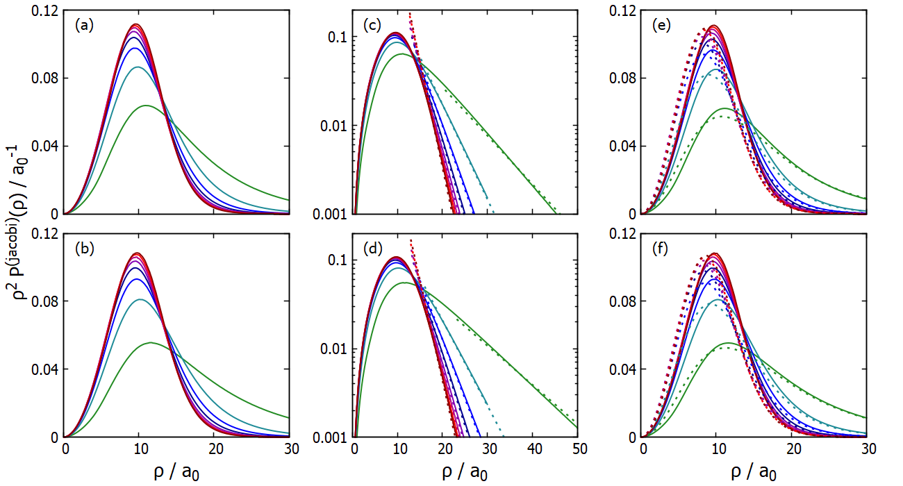
Figure 1: $\rho^{2}P_{N}^{(\text{jacobi})}(\rho)$ for $N=3-10$ at the physical point (top row) and at unitarity (bottom row). The solid lines in Figs. 1(a)-1(d) show $\rho^{2}P_{N}^{(\text{jacobi})}(\rho)$ for Model IB. At $\rho=20$ $a_{0}$, the curves are ordered, from top to bottom, from the smallest $N$ (the curve for $N=3$ is green) to the largest $N$ (the curve for $N=10$ is dark red). Note that the data shown in the first and second columns are identical but that the $x$- and $y$-scales differ. The dotted lines in Figs. 1(b) and 1(d) show the asymptotic behavior $A_{N}\exp(-2\kappa_{N}\rho)$, using the numerically determined binding momentum $\kappa_{N}$ and treating the “normalization constant” $A_{N}$ as a fitting parameter. The solid and dotted lines in Figs. 1(e)-1(f) (third column) show $\rho^{2}P_{N}^{(\text{jacobi})}(\rho)$ for Model IA and Model II, respectively. The agreement between the dotted and solid lines is excellent at large $\rho$ and deteriorates for smaller $\rho$. The deterioration is due to the inability of the low-energy model to fully capture the small length scale correlations. The color scheme used here is also used in Figs. 2, 3, 4(a), 6, 7, S3, and S4. The layout used here, i.e., the top row showing results at the physical point and the bottom row showing results at unitarity, is also used in Figs. 2, 5, 6, 7, and S4.

Figure 2 shows the scaled pair distribution functions $r^{2}P_{N}^{(2)}(r)$ for $N=2-10$ at the physical point (top row) and at unitarity (bottom row). The scaled pair distribution functions for the realistic interaction models display a clear maximum for $N\lesssim 6$. For larger $N$, the maximum broadens and shifts to larger $r$-values; for these larger $N$, the scaled pair distribution functions display a hint of a double-peak structure that can be interpreted as a signature of the development of a “second length scale or shell”. It is important to keep in mind that the clusters at the physical point and at unitarity are extremely floppy and diffuse and that the terms “second length scale” and “second shell” should be contextualized within the framework of extremely diffuse quantum liquids. The double-peak structure is not reproduced by the low-energy model (dotted lines in the third column).

The third column of Fig. 2 shows that the quantities $r^{2}P_{N}^{(2)}(r)$ for Model IA (solid lines) and Model II (dotted lines) differ for small $r$ ($r\lesssim 20$ $a_{0}$). Interestingly, the scaled pair distribution functions for the HFD-HE2 potential and the CPKMJS potential (solid lines) rise at about the same $r$-value for all $N$, namely at $r\approx 4.5$ $a_{0}$ or $r\approx 0.9$ $r_{\text{vdW}}$. Careful inspection shows that the rise is shifted to somewhat larger $r$-values for the clusters at unitarity interacting through realistic potentials than for the clusters at the physical point interacting through realistic potentials. The scaled pair distribution functions for the effective low-energy potential (Model II, dotted lines), in contrast, rise at much smaller $r$ values. The scaled pair distribution functions for Model I and Model II are different at small $r$ for two reasons: (i) The two-body Gaussian potential used in Model II does not have a hard wall at small $r$. (ii) Model II contains a repulsive three-body Gaussian potential, which alters the behavior when three particles are in close vicinity to each other, impacting the short-distance correlations of two-, three-, and higher-body subclusters.

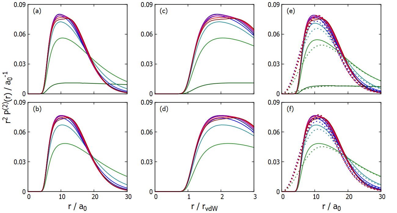
Figure 2: $r^{2}P_{N}^{(2)}(r)$ for $N=2-10$ at the physical point (top row) and for $N=3-10$ at unitarity (bottom row). The solid lines in Figs. 2(a)-2(d) show $r^{2}P_{N}^{(2)}(r)$ for Model IB. Note that the data shown in the first and second columns are identical: the first column shows $r$ in units of $a_{0}$ and the second column shows $r$ in units of $r_{\text{vdW}}$, focusing on the small-$r$ region. It can be seen that the scaled pair distribution functions for different $N$ collapse approximately for $r\approx r_{\text{vdW}}$. The solid and dotted lines in Figs. 1(e)-1(f) (third column) show $r^{2}P_{N}^{(2)}(r)$ for Model IA and Model II, respectively. Differences are most pronounced in the $r\lesssim 20$ $a_{0}$ region. The color scheme is the same as in Fig. 1.

To highlight the universality of the short-range behavior of the scaled pair distribution function $r^{2}P_{N}^{(2)}(r)$ for realistic interaction models, Fig. 3 replots $r^{2}P_{N}^{(2)}(r)$ at the physical point—including the factor $C_{N}^{(2)}$—for Model IA (dash-dotted lines) and Model IB (solid lines). As discussed in Sec. II, the two-body contact $C_{N}^{(2)}$ is determined by fitting the $N>2$ curves for small $r$ to the $N=2$ curve. It can be seen that the rise of the scaled curves collapses for $N=2-10$ in the regime $r\lesssim 1.4$ $r_{\text{vdW}}$ separately for both interaction models. The fact that the curves for each of the interaction models collapse confirms that the two-body contact $C_{N}^{(2)}$, determined in the manner described in Sec. II, provides a meaningful characterization of the short-distance behavior of van der Waals clusters.

Table S3 reports $C_{N}^{(2)}$ for helium clusters with $N=3-10$ interacting through Model IA-IC at the physical point. The ratio of $C_{N}^{(2)}$, $N\geq 3$, for two different interaction potentials is approximately constant. To leading order, this ratio is given by the ratio of $a_{s}/r_{\text{vdW}}$ for the two different interaction potentials. Specifically, the values for the HFD-HE2 potential are between $1.32$ and $1.38$ times larger than those for the CPKMJS potential; for comparison, $(a_{s}/r_{\text{vdW}})_{\text{HFD-HE2}}/(a_{s}/r_{\text{vdW}})_{\text{CPKMJS}}$ is equal to $1.40$. Those for the TTY potential are between $1.09$ and $1.10$ times larger than those for the CPKMJS potential; for comparison, $(a_{s}/r_{\text{vdW}})_{\text{TTY}}/(a_{s}/r_{\text{vdW}})_{\text{CPKMJS}}$ is equal to $1.10$.

To understand this behavior, we recall that the pair distribution functions for the realistic interaction potentials at the physical point are, for $N\gtrsim 5$, to a very good approximation independent of the potential model [compare, e.g., the solid lines in Figs. 2(a) and 2(e)]. The $N=2$ pair distribution functions, in contrast, differ notably. Because of this, the difference between the contacts $C_{N}^{(2)}$, $N\gtrsim 5$, for Model IA and Model IB predominantly reflects the difference between the respective $N=2$ pair distribution functions. Specifically, using the fact that the dimers are weakly bound and the pair distribution functions are normalized, the difference in the height of $r^{2}P_{2}^{(2)}(r)$ at small $r$ for different realistic potential models can be expressed in terms of the binding momentum and thus, using effective range theory, in terms of $a_{s}/r_{\text{vdW}}$. Assuming that the pair distribution functions for different potential models agree for larger $N$, we find that the ratio of the two-body contacts for larger $N$ is given, to leading order, by the ratio between $a_{s}/r_{\text{vdW}}$ for the two interaction potentials. Our analysis indicates that the $N$-dependence of the two-body contact $C_{N}^{(2)}$ for helium clusters at the physical point interacting through one realistic interaction model is, to a fairly good approximation, universally linked to that for helium clusters interacting through another realistic interaction model. The arguments presented here are reminiscent of the discussion of effective range corrections to the asymptotic normalization constant, which is defined by relating the “true” nuclear wave function to a wave function that is calculated assuming that the effective interaction in the asymptotically dominant channel has vanishing range Kim and Tubis (1974); Friar et al. (1982).

Table S3 also compares our results with those obtained in Ref. Bazak et al. (2020) for the LM2M2 potential. The $C_{N}^{(2)}$ values for the LM2M2 potential are between $1.06$ and $1.08$ times larger than those for the CPKMJS potential; this is quite a bit smaller than $(a_{s}/r_{\text{vdW}})_{\text{LM2M2}}/(a_{s}/r_{\text{vdW}})_{\text{CPKMJS}}=1.13$. We expect that the LM2M2 data from Ref. Bazak et al. (2020) would follow the same trends as displayed by our data; we speculate that the differences might be related to the different data analysis strategies employed.

Last, we note that our analysis of the short-distance behavior of the scaled pair distribution functions for the effective low-energy Model II reveals that the small-$r$ behaviors of $r^{2}P_{2}^{(2)}(r)$ and $r^{2}P_{N}^{(2)}(r)$ with $N\geq 3$ do not collapse as neatly by introducing an $r$-independent scaling factor for each $N$ (see Fig. S3 from the Supplemental Material) as the corresponding data for the realistic interaction models. Due to the presence of the repulsive three-body potential, the low-energy model does not capture the small-$r$, “high-energy” van der Waals universality of the pair distribution function.

The fact that the curves for Model IA in Fig. 3 are pushed to larger $r$ compared to those for Model IB can be interpreted as being due to Model IA being characterized by a larger effective repulsion than Model IB: the two-body $s$-wave scattering length for Model IA is larger than that for Model IB ($a_{s}=234.84$ $a_{0}$ compared to $a_{s}=170.86$ $a_{0}$). Interestingly, the rise of the scaled pair distribution functions is captured quantitatively by the universal van der Waals function $\varphi_{\text{vdW}}(r)$ Flambaum et al. (1999); Gao (1998),

$$\varphi_{\text{vdW}}(r)=B\bigg{[}\Gamma(5/4)x^{1/2}J_{1/4}(2x^{-2})-$$

$$\frac{r_{\text{vdW}}}{a_{s}}\Gamma(3/4)x^{1/2}J_{-1/4}(2x^{-2})\bigg{]},$$ (28)

which is obtained by solving the scaled radial Schrödinger equation for a purely attractive $-C_{6}/r^{6}$ potential. In Eq. (III), $x$ is equal to $r/r_{\text{vdW}}$. Thin black dash-dotted and solid lines in Fig. 3 show the quantity $|\varphi_{\text{vdW}}(r)|^{2}$ for Model IA ($a_{s}/r_{\text{vdW}}=46.95$) and Model IB ($a_{s}/r_{\text{vdW}}=33.63$), respectively. The nodes of the wave function $\varphi_{\text{vdW}}(r)$ in the $r\lesssim r_{\text{vdW}}$ region reflect the presence of deep-lying two-body bound states. For $r$-values beyond the last node, the density $|\varphi_{\text{vdW}}(r)|^{2}$ agrees well with $r^{2}P_{2}^{(2)}(r)/C_{N}^{(2)}$. For the infinite scattering length case, Refs. Naidon et al. (2014a, b) established the van der Waals universality of the short-distance correlations of the scaled pair distribution function of trimers interacting through realistic interaction potentials. Figure 3 shows that $|\varphi_{\text{vdW}}(r)|^{2}$ captures the short-distance correlations of $r^{2}P_{N}^{(2)}(r)$ also for helium clusters at the physical point.

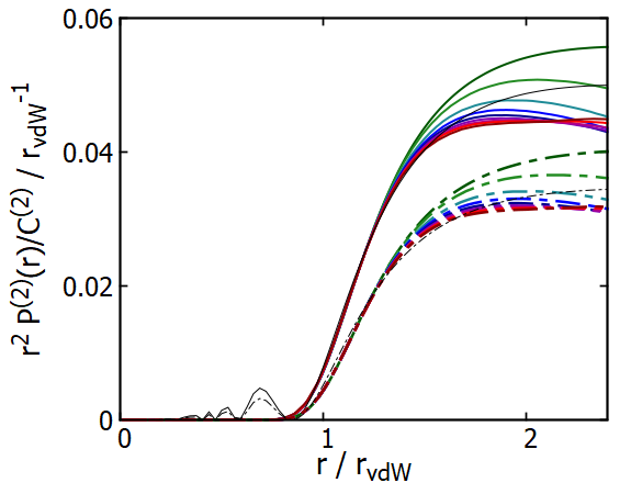
Figure 3: $r^{2}P_{N}^{(2)}(r)/C_{N}^{(2)}$, $N=2-10$, for two realistic interaction potentials at the physical point. The sets of dash-dotted and solid lines show results for Model IA and Model IB, respectively. The color scheme is the same as in Fig. 1. The thin black dash-dotted and solid lines show the universal van der Waals function $|\varphi_{\text{vdW}}(r)|^{2}$, Eq. (III), for Model IA and Model IB, respectively (these two models are characterized by slightly different $r_{\text{vdW}}$); the normalization constant $B$ is adjusted by fitting $|\varphi_{\text{vdW}}(r)|^{2}$ to $r^{2}P_{2}^{(2)}(r)$, including $r$ values ($r\lesssim 2r_{\text{vdW}}$) for which $P_{2}^{(2)}(r)$ takes values that are larger than 5 % and smaller than the maximum of $P_{2}^{(2)}(r)$ for Model IA and smaller than 95 % of the maximum of $P_{2}^{(2)}(r)$ for Model IB, respectively.

Figures 4 and 5 as well as Fig. S4 in the Supplemental Material summarize the three-body correlations of $N$-atom clusters. Figure S4, which shows the quantity $(\rho_{3})^{2}P_{N}^{(3,\text{jacobi})}(\rho_{3})$, highlights two key points. First, the scaled three-body distributions $(\rho_{3})^{2}P_{N}^{(3,\text{jacobi})}(\rho_{3})$ for Model IB and Model II (first and third columns) are visually indistinguishable, including in the small $\rho_{3}$ region; this is in clear contrast to the behavior of the scaled pair distribution functions. Second, the quantity $(\rho_{3})^{2}P_{N}^{(3,\text{jacobi})}(\rho_{3})$ becomes narrower as $N$ changes from $N=3$ to $N=4$ to $N=5$ but changes comparatively little for $N=6-10$. This indicates that the correlations of the three-body sub-system saturate approximately for these $N$-values. This “saturation” is different from the behavior of the scaled pair distribution functions, which show a more pronounced $N$ dependence for $N=6-10$.

Figure 4(a) focuses on the small $\rho_{3}$ behavior at the physical point. The solid and dash-dotted lines show $[(\rho_{3})^{2}P_{N}^{(3,\text{jacobi})}(\rho_{3})/C_{N}^{(2+1)}]/r_{\text{vdW}}^{-1}$ for $N=3-10$ for Model IA and Model II, respectively; to make the figure, the $x$- and $y$-axis are scaled using the van der Waals length $r_{\text{vdW}}$ for the HFD-HE2 potential (Model IA). The collapse of the scaled distribution functions is extremely clean for the realistic interaction potential (solid lines) and very clean for the low-energy potential (dash-dotted lines). Differences between the scaled curves for the realistic and low-energy models are clearly visible for small $\rho_{3}$. Figures 4(b) and 4(c) show the $N$-dependence of the $(2+1)$ contact $C_{N}^{(2+1)}$ at the physical point and at unitarity, respectively, for three different interaction potentials. The overall trends are the same for all three interaction potentials: $C_{N}^{(2+1)}$ increases for $N\lesssim 6$ or $7$ and then slowly decreases. The contacts $C_{N}^{(2+1)}$ for the low-energy model (triangles) are notably larger for $N\geq 4$ than those for the realistic potentials (squares and circles). Interestingly, while the contacts $C_{N}^{(2+1)}$ for the two realistic potentials (Model IA and Model IB) differ by a small amount for $N\geq 4$ at the physical point, they coincide, within our numerical accuracy, at unitarity (see numerical values of $C_{N}^{(2+1)}$ are collected in Table S4 This behavior of the contact is related to the three-body energies. The ratio $E_{\text{CPKMJS}}/E_{\text{HFD-HE2}}$ is equal to $1.12$ at the physical point (see Table 1) and $1.00$ at unitarity (see Table 2).

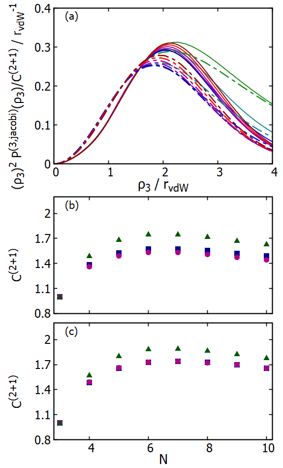
Figure 4: Triple correlations and $(2+1)$ contact. (a) The solid and dash-dotted lines show $(\rho_{3})^{2}P_{N}^{(3,\text{jacobi})}(\rho_{3})/C_{N}^{(2+1)}$ for the realistic HFD-HE2 potential (Model IA) and the effective low-energy potential (Model II), respectively, at the physical point for $N=3-10$. The color scheme is the same as in Fig. 1. (b) The squares, circles, and triangles show the pair contact $C_{N}^{(2+1)}$ at the physical point as a function of $N$ for Model IA, Model IB, and Model II, respectively. (c) The squares, circles, and triangles show the pair contact $C_{N}^{(2+1)}$ at unitarity as a function of $N$ for Model IA, Model IB, and Model II, respectively.

As already mentioned in Sec. II, the $(2+1)$ contact investigated here differs from the three-body contact investigated in Ref. Werner and Castin (2012b); Braaten et al. (2011) at the physical point. While the three-body contact for realistic interaction models is, to a large degree, governed by the short-distance two-body correlations, the three-body contact for the low-energy model depends notably on the repulsive three-body potential. The $(2+1)$ contact, in contrast, captures the behavior as a third particle approaches the center-of-mass of a two-body sub-unit of any size. As such, the $(2+1)$ contact probes, on average, larger length scales than the three-body contact. Correspondingly, the low-energy model does a better job of reproducing the $(2+1)$ contact obtained for the realistic potentials than it does of reproducing the three-body contact obtained for the realistic potentials (we are not showing data for the three-body contact).

To gain insights into the distribution of the shapes that the triples are arranged in, the first, second, and third columns of Fig. 5 show the distribution function $P_{N}^{(3,\text{shape})}(\bar{x},\bar{y})$ for $N=3$, $N=4$, and $N=10$, respectively. We observe that the distributions, and thus the structures, at the physical point (top row) and at unitarity (bottom row) are very similar. The highest probability is found at $\bar{x}=0$ and $\bar{y}\approx 0.35$, which corresponds to a slightly elongated triangle. Even though the distributions have a maximum, the clusters’ wave functions include essentially all shapes, except for those where two particles sit on top of each other ($\bar{y}=0$ and arbitrary $\bar{x}$) and where the triangles are highly elongated ($\bar{y}\approx 0$ and $\bar{x}\approx\pm 0.5$). Figure 5 shows that the distributions become more peaked with increasing $N$ and that the likelihood to find highly-elongated triangles becomes smaller with increasing $N$.

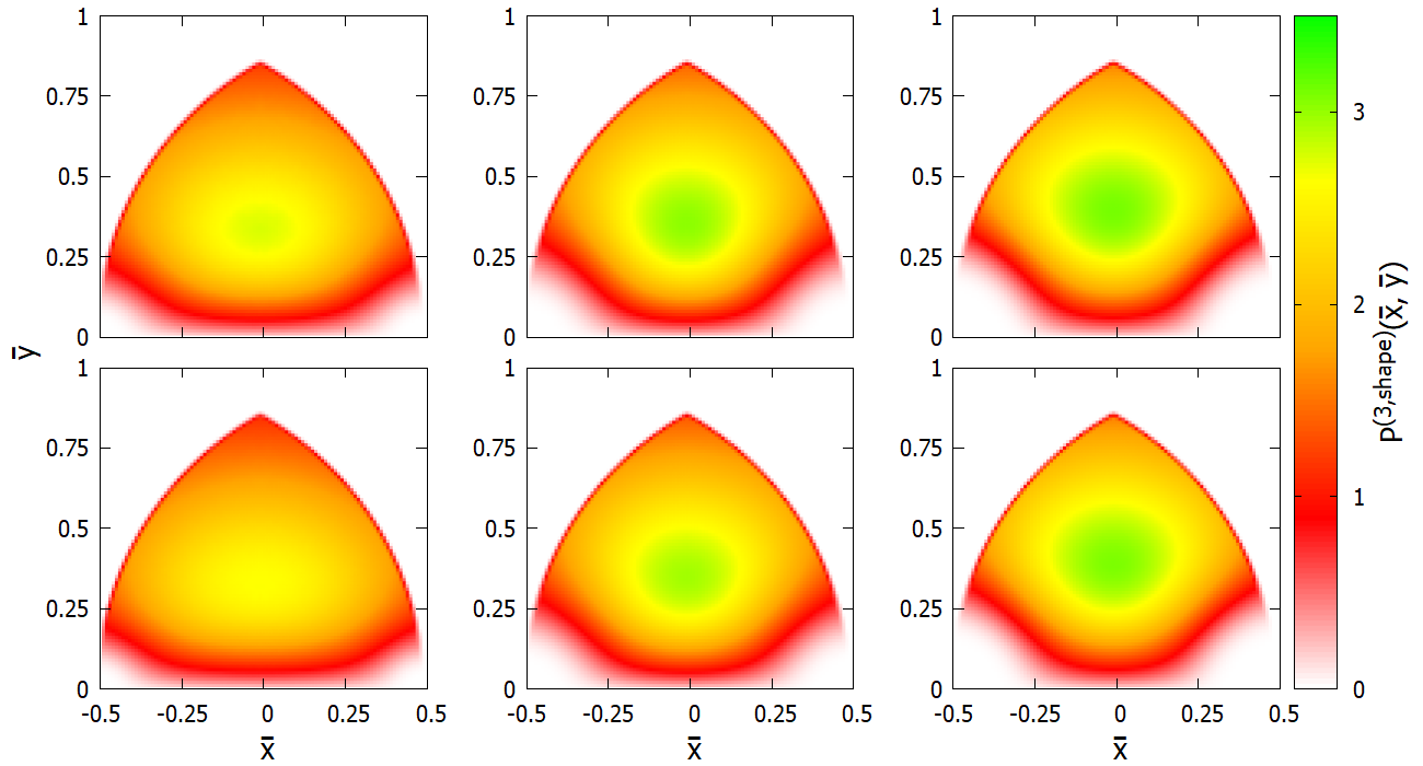
Figure 5: $P_{N}^{(3,\text{shape})}(\bar{x},\bar{y})$ for Model IB at the physical point (top row) and at unitarity (bottom row). The first, second, and third columns show results for $N=3$, $N=4$, and $N=10$, respectively. The color bar on the right applies to all six panels. Since the triangles are oriented and normalized such that one particle sits at $(\bar{x},\bar{y})=(-1/2,0)$ and the other at $(\bar{x},\bar{y})=(+1/2,0)$ (with the interparticle distance vector corresponding to the largest distance being oriented along the $\pm\bar{x}$-axis), the regions in the top left and top right of the panels are excluded by construction.

Figures 6(a) and 6(b) show the scaled hyperradial density $(\rho_{N})^{3N-4}P_{N}^{(\text{hyper})}(\rho_{N})$ for $N=3-10$ clusters interacting through the CPKMJS potential at the physical point and at unitarity, respectively. The differences between the scaled hyperradial densities at the physical point and at unitarity for fixed $N$ are small. Careful inspection shows that the scaled hyperradial densities at unitarity extend to larger $\rho_{N}$ and rise at slightly larger $\rho_{N}$ than those at the physical point. Correspondingly, the maximum of $(\rho_{N})^{3N-4}P_{N}^{(\text{hyper})}(\rho_{N})$ is located at slightly larger $\rho_{N}$ for the clusters at unitarity than for the clusters at the physical point. The fact that the scaled hyperradial densities at unitarity extend to larger $\rho_{N}$ than those at the physical point is a consequence of the smaller binding energy at unitarity than at the physical point. As $N$ increases, the scaled hyperradial densities become more localized, with their maximum shifting to larger $\rho_{N}$. To interpret this behavior, one needs to keep in mind that the definition of the hyperradius is intimately linked to the definition of the hyperradial mass $M$. Since the quantity $M\rho_{N}^{2}$ is an invariant but not $\rho_{N}$ and $M$ separately, $\rho_{N}$ can be multiplied by an overall factor Lin (1995); Blume and Greene (2000); D’Incao (2018). If all interparticle distances were equal to $\bar{r}$, then $\rho_{N}$ [as defined in Eq. (24)] would approach $\bar{r}/\sqrt{2}$ in the $N\rightarrow\infty$ limit. Since helium clusters behave roughly as incompressible liquids, the maximum of the hyperradial density is expected to occur at increasingly larger $\rho_{N}$ as $N$ increases. Figures 6(a) and 6(b) confirm this notion.

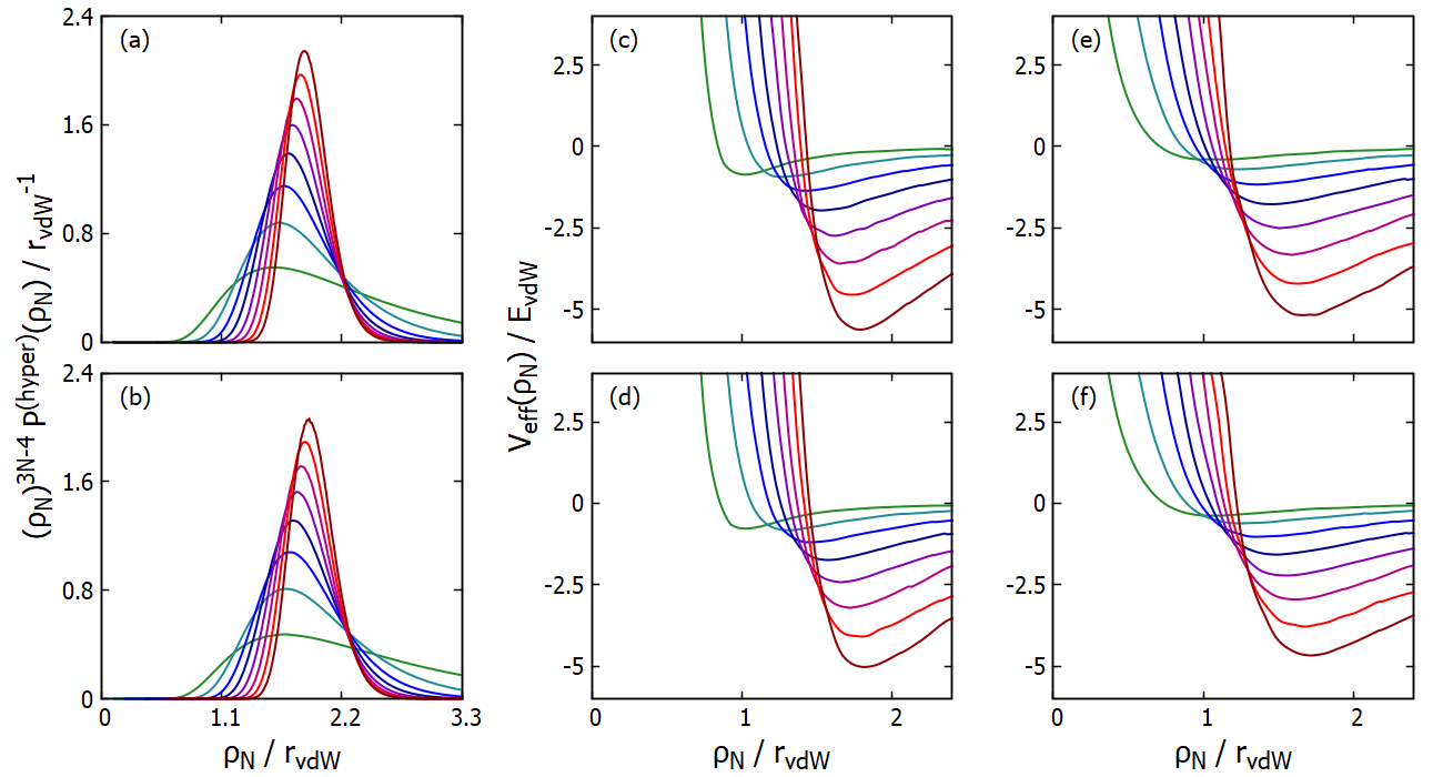
Figure 6: Hyperradial properties for $N=3-10$ at the physical point (top row) and at unitarity (bottom row). The first column shows $P_{N}^{(\text{hyper})}(\rho_{N})$ for Model IA. The second column shows the (approximate) effective potential curves $V_{\text{eff}}(\rho_{N})$ for Model IA, calculated using Eq. (29). For comparison, the third column shows $V_{\text{eff}}(\rho_{N})$ for Model II (the Model II plots are made using the van der Waals length for Model IA as a scale). The color scheme is the same as in Fig. 1.

We now use the hyperradial densities to calculate approximate hyperradial potential curves. We note that Ref. Blume and Greene (2000) obtained the effective hyperradial potential curves of helium clusters with $N=3-10$ at the physical point following an alternative and more rigorous approach; in addition, Ref. Blume and Greene (2000) presented careful benchmark calculations of the different approaches for $N=3$. The approach pursued here yields potential curves that agree semi-quantitatively with the more accurate potential curves presented in Ref. Blume and Greene (2000). If the hyperradial and hyperangular degrees of freedom separate, the effective one-dimensional Schroedinger equation for the lowest effective hyperradial potential curve $V_{\text{eff}}(\rho_{N})$ can be written in terms of $F_{N}(\rho_{N})$ Castin (2004); Werner and Castin (2006); Jonsell et al. (2002); Hiyama and Kamimura (2014); Werner and Castin (2012b),

$$\left[-\frac{\hbar^{2}}{2M}\frac{\partial^{2}}{\partial\rho_{N}^{2}}+V_{\text{eff}}(\rho_{N})\right]F_{N}(\rho_{N})=E_{N}F_{N}(\rho_{N}),$$ (29)

where $F_{N}(\rho_{N})=[(\rho_{N})^{3N-4}P_{N}^{(\text{hyper})}(\rho_{N})]^{1/2}$. For the $N$-particle clusters ($N\geq 3$) at unitarity, the separability is broken due to the finite-range nature of the two-body interactions. At the physical point, the finiteness of the scattering length provides an additional separability-breaking mechanism. Even though Eq. (29) is not strictly valid for the potential models considered in this work, we “invert” it to obtain approximate effective hyperradial potentials $V_{\text{eff}}(\rho_{N})$. The same strategy was pursued in Ref. Hiyama and Kamimura (2014) for $N=3$ and $4$. Figures 6(c) and 6(d) show the results for Model IB at the physical point and at unitarity, respectively. The differences between the potential curves at the physical point and at unitarity are very small. Reference Hiyama and Kamimura (2014) conjectured, based on results for $N=3$ and $N=4$, that the location of the repulsive inner wall of the hyperradial potential curves varies as $(N-1)r_{\text{vdW}}/\sqrt{2N}$; this scaling accounts for an effective non-trivial reduction of the configuration space due to an energy cost associated with adiabatic deformation Naidon et al. (2014a, b). This scaling was contrasted with an alternative scaling of $\sqrt{N-1}r_{\text{vdW}}/\sqrt{2N}$, which arises assuming that the minimum average interparticle spacing is given by $r_{\text{vdW}}$. For $N=10$, the inner wall would be located, according to these two scalings, at $0.671r_{\text{vdW}}$ and $2.01r_{\text{vdW}}$. Figures 6(c) and 6(d) show that the scaling is somewhere in between.

The corresponding effective hyperradial potential curves for Model II are shown in Figs. 6(e) and 6(f). The effective potential curves for Model II are significantly softer (less steep) at small $\rho_{N}$ ($\rho_{N}/r_{\text{vdW}}$ between about $0.6$ and $1.2$) than those for Model IB; this is consistent with what was discussed above for the pair distribution functions.

Last, Fig. 7 presents the KER distribution functions at the physical point (top row) and at unitarity (bottom row). While small helium clusters have been isolated in molecular beam experiments Voigtsberger et al. (2014); Kunitski et al. (2015), Coulomb explosion experiments for $N\gtrsim 4$ are expected to be complicated by the fact the ions leaving the helium clusters might be undergoing additional collisions Ulrich et al. (2011); Kazandjian et al. (2018). Despite of this challenge, we find it useful to analyze the dependence of the KER distribution functions on the various interaction models. Since the number of interparticle distances increases as $N^{2}$ with increasing $N$, the KER distribution functions move to larger KER with increasing $N$. The KER distribution functions for Model IA (first column) and Model IB (second column) are nearly indistinguishable on the scale shown. Careful inspection reveals small differences between the KER distribution functions of clusters interacting through realistic interaction potentials at the physical point and at unitarity.

The KER distribution functions for clusters interacting through Model II extend to significantly larger KER; this behavior is linked to the enhanced probability for clusters interacting through Model II, relative to those interacting through realistic interaction potentials (Model I), to find two particles at small interparticle distances. The broader KER distribution functions for Model II also lead to peak values of the KER distribution functions compared to those for Model I. We note that the KER distribution functions for Model II do not only differ in the tail region from those for Model I (high-energy region or short-distance region) but also in the “rising portion” of the KER distribution function (large distance region); these deviations are more pronounced for larger $N$ than for smaller $N$. The deviations arise because the KER distribution functions in the rising portion are not dominated by configurations in which all interparticle distances are large but by configurations where $N-1$ interparticle distances are large and the remaining $N(N-1)/2-(N-1)$ interparticle distances are not particularly large.

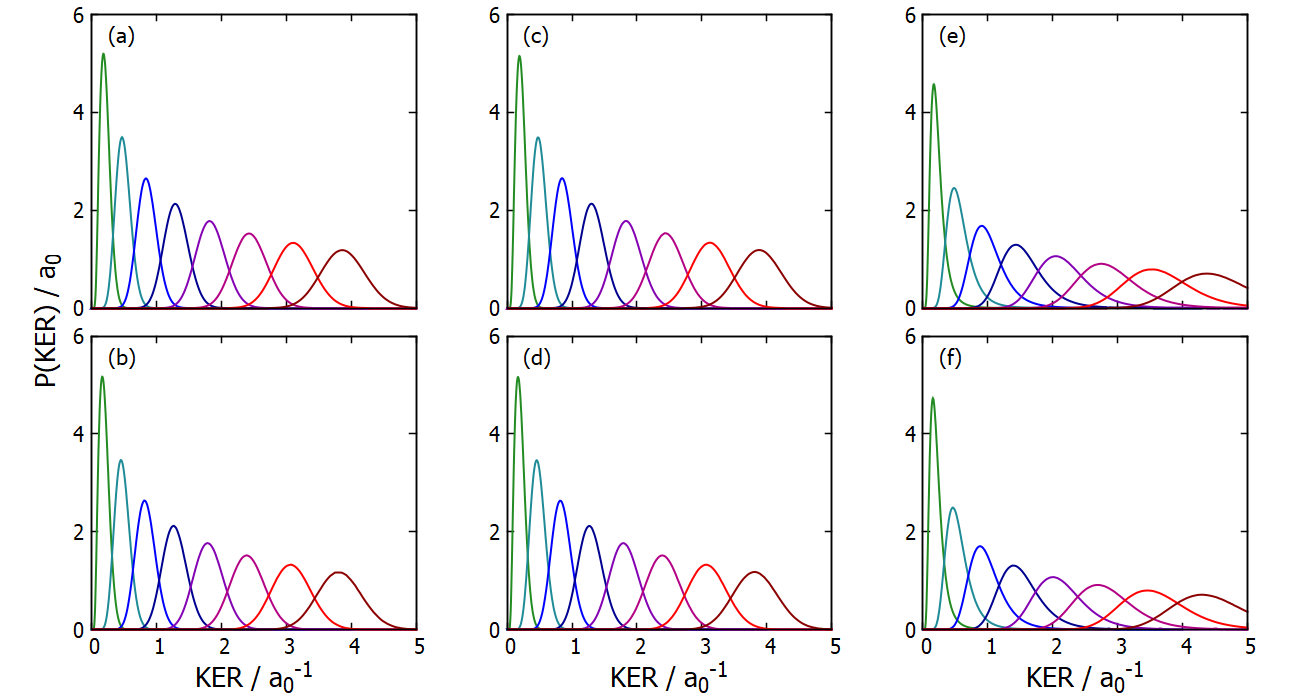
Figure 7: KER for $N=3-10$ at the physical point (top row) and at unitarity (bottom row). The first, second, and third columns show the KER for Model IA, Model IB, and Model II, respectively. The color scheme is the same as in Fig. 1.

IV Conclusions

This paper presented a comprehensive study of the structural properties of small bosonic helium clusters consisting of up to $N=10$ atoms and interacting through realistic interaction potentials. In addition to helium clusters at the physical point, characterized by a two-body $s$-wave scattering length that is positive and finite (and notably larger than the van der Waals length), clusters interacting with an infinite $s$-wave scattering were investigated. To reach unitarity, the realistic helium-helium interaction potential was multiplied by an overall factor that is close to but smaller than one.

For comparison, the properties of the systems at the physical point and at unitarity were also calculated for an effective low-energy interaction model that was introduced in the literature Kievsky et al. (2020). The model’s strictly attractive two-body potential reproduces the two-body $s$-wave scattering length and two-body binding energy obtained for the HFD-HE2 potential. A strictly repulsive three-body potential is added to reproduce the three- and four-body energies obtained for the HFD-HE2 potential. Importantly, there is a difference between the effective low-energy model construction for clusters at the physical point and at unitarity. At the physical point, the requirements for matching the two-body $s$-wave scattering length and two-body binding energy are two distinct requirements. At unitarity, in contrast, the two requirements are equivalent, i.e., fulfilling one of these requirements implies that the other requirement is fulfilled automatically.

A detailed analysis of the structural properties at small and large length scales was presented, with focus on comparing the results for different realistic interaction potentials and those for the HFD-HE2 potential and the effective low-energy model. Several small distance behaviors were found to be described accurately by the two-body correlation function for a purely attractive $-C_{6}/r^{6}$ potential. The small length scale behavior of the pair distribution functions for the realistic interaction models at the physical point was summarized by the two-body contact and the $(2+1)$ contact for each cluster size. The two-body contacts for different realistic interaction potentials were found to be related to each other through, roughly, $N$-independent scaling factors. Following the spirit of Ref. Bazak et al. (2020), it would be interesting to extend the current study to larger clusters and to extract, using the liquid drop model, the bulk pair-atom contact both at the physical point and at unitarity. It would also be interesting to investigate mixed clusters that contain bosonic ⁴He and fermionic ³He atoms.

Acknowledgement: Support by the National Science Foundation through grant numbers PHY-1806259 and PHY-2110158 is gratefully acknowledged. Work during the early stage was additionally supported by grant number NSF-1659501. This work used the OU Supercomputing Center for Education and Research (OSCER) at the University of Oklahoma (OU).

References

- Pandharipande et al. (1986) V. R. Pandharipande, S. C. Pieper, and R. B. Wiringa, Phys. Rev. B 34, 4571 (1986), URL https://link.aps.org/doi/10.1103/PhysRevB.34.4571.
- Pandharipande et al. (1983) V. R. Pandharipande, J. G. Zabolitzky, S. C. Pieper, R. B. Wiringa, and U. Helmbrecht, Phys. Rev. Lett. 50, 1676 (1983), URL https://link.aps.org/doi/10.1103/PhysRevLett.50.1676.
- Barnett and Whaley (1993) R. N. Barnett and K. B. Whaley, Phys. Rev. A 47, 4082 (1993), URL https://link.aps.org/doi/10.1103/PhysRevA.47.4082.
- Lim et al. (1977) T. K. Lim, S. K. Duffy, and W. C. Damer, Phys. Rev. Lett. 38, 341 (1977), URL https://link.aps.org/doi/10.1103/PhysRevLett.38.341.
- Cornelius and Glöckle (1986) T. Cornelius and W. Glöckle, The Journal of Chemical Physics 85, 3906 (1986), eprint https://doi.org/10.1063/1.450912, URL https://doi.org/10.1063/1.450912.
- Whaley (1994) K. B. Whaley, International Reviews in Physical Chemistry 13, 41 (1994), eprint https://doi.org/10.1080/01442359409353290, URL https://doi.org/10.1080/01442359409353290.
- Lewerenz (1997) M. Lewerenz, The Journal of Chemical Physics 106, 4596 (1997), eprint https://doi.org/10.1063/1.473501, URL https://doi.org/10.1063/1.473501.
- Esry et al. (1996) B. D. Esry, C. D. Lin, and C. H. Greene, Phys. Rev. A 54, 394 (1996), URL https://link.aps.org/doi/10.1103/PhysRevA.54.394.
- Guardiola et al. (2006) R. Guardiola, O. Kornilov, J. Navarro, and J. Peter Toennies, The Journal of Chemical Physics 124, 084307 (2006), eprint https://doi.org/10.1063/1.2140723, URL https://doi.org/10.1063/1.2140723.
- Toennies (2013) J. P. Toennies, Molecular Physics 111, 1879 (2013), eprint https://doi.org/10.1080/00268976.2013.802039, URL https://doi.org/10.1080/00268976.2013.802039.
- Chin and Krotscheck (1995) S. A. Chin and E. Krotscheck, Phys. Rev. B 52, 10405 (1995), URL https://link.aps.org/doi/10.1103/PhysRevB.52.10405.
- Dalfovo et al. (1995) F. Dalfovo, A. Lastri, L. Pricaupenko, S. Stringari, and J. Treiner, Phys. Rev. B 52, 1193 (1995), URL https://link.aps.org/doi/10.1103/PhysRevB.52.1193.
- Kwon et al. (2000) Y. Kwon, P. Huang, M. V. Patel, D. Blume, and K. B. Whaley, The Journal of Chemical Physics 113, 6469 (2000), eprint https://doi.org/10.1063/1.1310608, URL https://doi.org/10.1063/1.1310608.
- Luo et al. (1996) F. Luo, C. F. Giese, and W. R. Gentry, The Journal of Chemical Physics 104, 1151 (1996), eprint https://doi.org/10.1063/1.470771, URL https://doi.org/10.1063/1.470771.
- Schöllkopf and Toennies (1994) W. Schöllkopf and J. P. Toennies, Science 266, 1345 (1994), eprint https://www.science.org/doi/pdf/10.1126/science.266.5189.1345, URL https://www.science.org/doi/abs/10.1126/science.266.5189.1345.
- Schöllkopf and Toennies (1996) W. Schöllkopf and J. P. Toennies, The Journal of Chemical Physics 104, 1155 (1996), eprint https://doi.org/10.1063/1.470772, URL https://doi.org/10.1063/1.470772.
- Grisenti et al. (2000) R. E. Grisenti, W. Schöllkopf, J. P. Toennies, G. C. Hegerfeldt, T. Köhler, and M. Stoll, Phys. Rev. Lett. 85, 2284 (2000), URL https://link.aps.org/doi/10.1103/PhysRevLett.85.2284.
- Braaten and Hammer (2003) E. Braaten and H.-W. Hammer, Phys. Rev. A 67, 042706 (2003), URL https://link.aps.org/doi/10.1103/PhysRevA.67.042706.
- Hiyama and Kamimura (2012a) E. Hiyama and M. Kamimura, Phys. Rev. A 85, 062505 (2012a), URL https://link.aps.org/doi/10.1103/PhysRevA.85.062505.
- Hiyama and Kamimura (2012b) E. Hiyama and M. Kamimura, Phys. Rev. A 85, 022502 (2012b), URL https://link.aps.org/doi/10.1103/PhysRevA.85.022502.
- Rama Krishna and Whaley (1990a) M. V. Rama Krishna and K. B. Whaley, The Journal of Chemical Physics 93, 6738 (1990a), eprint https://doi.org/10.1063/1.458943, URL https://doi.org/10.1063/1.458943.
- Barletta and Kievsky (2001) P. Barletta and A. Kievsky, Phys. Rev. A 64, 042514 (2001), URL https://link.aps.org/doi/10.1103/PhysRevA.64.042514.
- Nielsen et al. (1998) E. Nielsen, D. V. Fedorov, and A. S. Jensen, Journal of Physics B: Atomic, Molecular and Optical Physics 31, 4085 (1998), URL https://doi.org/10.1088/0953-4075/31/18/008.
- Blume et al. (2000) D. Blume, C. H. Greene, and B. D. Esry, The Journal of Chemical Physics 113, 2145 (2000), eprint https://doi.org/10.1063/1.482027, URL https://doi.org/10.1063/1.482027.
- Blume (2015) D. Blume, Few-Body Systems 56, 859 (2015), ISSN 1432-5411, URL https://doi.org/10.1007/s00601-015-0996-6.
- Kunitski et al. (2015) M. Kunitski, S. Zeller, J. Voigtsberger, A. Kalinin, L. P. H. Schmidt, M. Schöffler, A. Czasch, W. Schöllkopf, R. E. Grisenti, T. Jahnke, et al., Science 348, 551 (2015), eprint https://www.science.org/doi/pdf/10.1126/science.aaa5601, URL https://www.science.org/doi/abs/10.1126/science.aaa5601.
- Kolganova et al. (2011) E. A. Kolganova, A. K. Motovilov, and W. Sandhas, Few-Body Systems 51, 249 (2011), ISSN 1432-5411, URL https://doi.org/10.1007/s00601-011-0233-x.
- Stipanović et al. (2016) P. Stipanović, L. V. Markić, and J. Boronat, 49, 185101 (2016), URL https://doi.org/10.1088/0953-4075/49/18/185101.
- Naidon et al. (2012) P. Naidon, E. Hiyama, and M. Ueda, Phys. Rev. A 86, 012502 (2012), URL https://link.aps.org/doi/10.1103/PhysRevA.86.012502.
- Kievsky et al. (2014) A. Kievsky, N. K. Timofeyuk, and M. Gattobigio, Phys. Rev. A 90, 032504 (2014), URL https://link.aps.org/doi/10.1103/PhysRevA.90.032504.
- Kievsky et al. (2017) A. Kievsky, A. Polls, B. Juliá-Díaz, and N. K. Timofeyuk, Phys. Rev. A 96, 040501 (2017), URL https://link.aps.org/doi/10.1103/PhysRevA.96.040501.
- Blume and Greene (2000) D. Blume and C. H. Greene, The Journal of Chemical Physics 112, 8053 (2000), eprint https://doi.org/10.1063/1.481404, URL https://doi.org/10.1063/1.481404.
- Kievsky et al. (2020) A. Kievsky, A. Polls, B. Juliá-Díaz, N. K. Timofeyuk, and M. Gattobigio, Phys. Rev. A 102, 063320 (2020), URL https://link.aps.org/doi/10.1103/PhysRevA.102.063320.
- Bazak et al. (2020) B. Bazak, M. Valiente, and N. Barnea, Phys. Rev. A 101, 010501 (2020), URL https://link.aps.org/doi/10.1103/PhysRevA.101.010501.
- Przybytek et al. (2010) M. Przybytek, W. Cencek, J. Komasa, G. Łach, B. Jeziorski, and K. Szalewicz, Phys. Rev. Lett. 104, 183003 (2010), URL https://link.aps.org/doi/10.1103/PhysRevLett.104.183003.
- Zeller et al. (2016) S. Zeller, M. Kunitski, J. Voigtsberger, A. Kalinin, A. Schottelius, C. Schober, M. Waitz, H. Sann, A. Hartung, T. Bauer, et al., Proceedings of the National Academy of Sciences 113, 14651 (2016), ISSN 0027-8424, eprint https://www.pnas.org/content/113/51/14651.full.pdf, URL https://www.pnas.org/content/113/51/14651.
- Ceperley (1995) D. M. Ceperley, Rev. Mod. Phys. 67, 279 (1995), URL https://link.aps.org/doi/10.1103/RevModPhys.67.279.
- Pomorski and Dudek (2003) K. Pomorski and J. Dudek, Phys. Rev. C 67, 044316 (2003), URL https://link.aps.org/doi/10.1103/PhysRevC.67.044316.
- Feynman and Cohen (1956) R. P. Feynman and M. Cohen, Phys. Rev. 102, 1189 (1956), URL https://link.aps.org/doi/10.1103/PhysRev.102.1189.
- Henshaw and Woods (1961) D. G. Henshaw and A. D. B. Woods, Phys. Rev. 121, 1266 (1961), URL https://link.aps.org/doi/10.1103/PhysRev.121.1266.
- Rama Krishna and Whaley (1990b) M. V. Rama Krishna and K. B. Whaley, The Journal of Chemical Physics 93, 746 (1990b), eprint https://doi.org/10.1063/1.459525, URL https://doi.org/10.1063/1.459525.
- Grebenev et al. (1998) S. Grebenev, J. P. Toennies, and A. F. Vilesov, Science 279, 2083 (1998), eprint https://www.science.org/doi/pdf/10.1126/science.279.5359.2083, URL https://www.science.org/doi/abs/10.1126/science.279.5359.2083.
- Toennies and Vilesov (2004) J. P. Toennies and A. F. Vilesov, Angewandte Chemie International Edition 43, 2622 (2004), eprint https://onlinelibrary.wiley.com/doi/pdf/10.1002/anie.200300611, URL https://onlinelibrary.wiley.com/doi/abs/10.1002/anie.200300611.
- Mauracher et al. (2018) A. Mauracher, O. Echt, A. Ellis, S. Yang, D. Bohme, J. Postler, A. Kaiser, S. Denifl, and P. Scheier, Physics Reports 751, 1 (2018), ISSN 0370-1573, URL https://www.sciencedirect.com/science/article/pii/S0370157318301182.
- Bierau et al. (2010) F. Bierau, P. Kupser, G. Meijer, and G. von Helden, Phys. Rev. Lett. 105, 133402 (2010), URL https://link.aps.org/doi/10.1103/PhysRevLett.105.133402.
- Toennies et al. (2001) J. P. Toennies, A. F. Vilesov, and K. B. Whaley, Physics Today 54, 31 (2001), eprint https://doi.org/10.1063/1.1359707, URL https://doi.org/10.1063/1.1359707.
- Stienkemeier and Lehmann (2006) F. Stienkemeier and K. K. Lehmann, Journal of Physics B: Atomic, Molecular and Optical Physics 39, R127 (2006), URL https://doi.org/10.1088/0953-4075/39/8/r01.
- Callegari et al. (2001) C. Callegari, K. K. Lehmann, R. Schmied, and G. Scoles, The Journal of Chemical Physics 115, 10090 (2001), eprint https://aip.scitation.org/doi/pdf/10.1063/1.1418746, URL https://aip.scitation.org/doi/abs/10.1063/1.1418746.
- Toennies and Vilesov (1998) J. P. Toennies and A. F. Vilesov, Annual Review of Physical Chemistry 49, 1 (1998), pMID: 15012423, eprint https://doi.org/10.1146/annurev.physchem.49.1.1, URL https://doi.org/10.1146/annurev.physchem.49.1.1.
- Aziz et al. (1979) R. A. Aziz, V. P. S. Nain, J. S. Carley, W. L. Taylor, and G. T. McConville, The Journal of Chemical Physics 70, 4330 (1979), eprint https://doi.org/10.1063/1.438007, URL https://doi.org/10.1063/1.438007.
- Cencek et al. (2012) W. Cencek, M. Przybytek, J. Komasa, J. B. Mehl, B. Jeziorski, and K. Szalewicz, The Journal of Chemical Physics 136, 224303 (2012), eprint https://doi.org/10.1063/1.4712218, URL https://doi.org/10.1063/1.4712218.
- Tang et al. (1995) K. T. Tang, J. P. Toennies, and C. L. Yiu, Phys. Rev. Lett. 74, 1546 (1995), URL https://link.aps.org/doi/10.1103/PhysRevLett.74.1546.
- Naidon et al. (2014a) P. Naidon, S. Endo, and M. Ueda, Phys. Rev. Lett. 112, 105301 (2014a), URL https://link.aps.org/doi/10.1103/PhysRevLett.112.105301.
- Naidon et al. (2014b) P. Naidon, S. Endo, and M. Ueda, Phys. Rev. A 90, 022106 (2014b), URL https://link.aps.org/doi/10.1103/PhysRevA.90.022106.
- Tan (2008a) S. Tan, Annals of Physics 323, 2987 (2008a), ISSN 0003-4916, URL https://www.sciencedirect.com/science/article/pii/S0003491608000420.
- Tan (2008b) S. Tan, Annals of Physics 323, 2971 (2008b), ISSN 0003-4916, URL https://www.sciencedirect.com/science/article/pii/S0003491608000432.
- Tan (2008c) S. Tan, Annals of Physics 323, 2952 (2008c), ISSN 0003-4916, URL https://www.sciencedirect.com/science/article/pii/S0003491608000456.
- Werner and Castin (2012a) F. Werner and Y. Castin, Phys. Rev. A 86, 013626 (2012a), URL https://link.aps.org/doi/10.1103/PhysRevA.86.013626.
- Werner and Castin (2012b) F. Werner and Y. Castin, Phys. Rev. A 86, 053633 (2012b), URL https://link.aps.org/doi/10.1103/PhysRevA.86.053633.
- Braaten et al. (2011) E. Braaten, D. Kang, and L. Platter, Phys. Rev. Lett. 106, 153005 (2011), URL https://link.aps.org/doi/10.1103/PhysRevLett.106.153005.
- Weiss et al. (2015a) R. Weiss, B. Bazak, and N. Barnea, Phys. Rev. Lett. 114, 012501 (2015a), URL https://link.aps.org/doi/10.1103/PhysRevLett.114.012501.
- Weiss et al. (2015b) R. Weiss, B. Bazak, and N. Barnea, Phys. Rev. C 92, 054311 (2015b), URL https://link.aps.org/doi/10.1103/PhysRevC.92.054311.
- Miller (2018) G. A. Miller, Physics Letters B 777, 442 (2018), ISSN 0370-2693, URL https://www.sciencedirect.com/science/article/pii/S0370269318300030.
- Hen et al. (2014) O. Hen, M. Sargsian, L. B. Weinstein, E. Piasetzky, H. Hakobyan, D. W. Higinbotham, M. Braverman, W. K. Brooks, S. Gilad, K. P. Adhikari, et al., Science 346, 614 (2014), eprint https://www.science.org/doi/pdf/10.1126/science.1256785, URL https://www.science.org/doi/abs/10.1126/science.1256785.
- Cruz-Torres et al. (2021) R. Cruz-Torres, D. Lonardoni, R. Weiss, M. Piarulli, N. Barnea, D. W. Higinbotham, E. Piasetzky, A. Schmidt, L. B. Weinstein, R. B. Wiringa, et al., Nature Physics 17, 306 (2021), ISSN 1745-2481, URL https://doi.org/10.1038/s41567-020-01053-7.
- Odell et al. (2021) D. Odell, A. Deltuva, and L. Platter, Phys. Rev. A 104, 023306 (2021), URL https://link.aps.org/doi/10.1103/PhysRevA.104.023306.
- (67) We use (the last digit is rounded). This agrees with the value used by Hiyama and Kamimura Hiyama and Kamimura (2012a) but is about % smaller than the value used by Kievsky et al. Kievsky et al. (2020). For the HFD-HE2 potential, this difference translates to differences in the two-body -wave scattering length and the two-, three-, and four-body energies that are larger than our numerical uncertainties. Using Kievsky et al. (2020), we find—in agreement with Ref. Kievsky et al. (2020)— , which is % larger than the value reported in the main part of this paper. ().
- (68) We note that the definition of the model in Ref. Kievsky et al. (2020) contains a typo: Reference Kievsky et al. (2020) reports as being positive; it is, however, negative. Our is related to through . ().
- Yan and Blume (2015) Y. Yan and D. Blume, Phys. Rev. A 92, 033626 (2015), URL https://link.aps.org/doi/10.1103/PhysRevA.92.033626.
- von Stecher (2010) J. von Stecher, Journal of Physics B: Atomic, Molecular and Optical Physics 43, 101002 (2010), URL https://doi.org/10.1088/0953-4075/43/10/101002.
- Janzen and Aziz (1995) A. R. Janzen and R. A. Aziz, The Journal of Chemical Physics 103, 9626 (1995), eprint https://doi.org/10.1063/1.469978, URL https://doi.org/10.1063/1.469978.
- Braaten and Hammer (2006) E. Braaten and H.-W. Hammer, Physics Reports 428, 259 (2006), ISSN 0370-1573, URL https://www.sciencedirect.com/science/article/pii/S0370157306000822.
- Braaten and Hammer (2007) E. Braaten and H.-W. Hammer, Annals of Physics 322, 120 (2007), ISSN 0003-4916, january Special Issue 2007, URL https://www.sciencedirect.com/science/article/pii/S0003491606002387.
- Naidon and Endo (2017) P. Naidon and S. Endo, Reports on Progress in Physics 80, 056001 (2017), URL https://doi.org/10.1088/1361-6633/aa50e8.
- Platter et al. (2009) L. Platter, C. Ji, and D. R. Phillips, Phys. Rev. A 79, 022702 (2009), URL https://link.aps.org/doi/10.1103/PhysRevA.79.022702.
- (76) For the interaction potentials of Model I-type, the effective range is, in the large regime, roughly three times as large as the van der Waals length . ().
- Kosztin et al. (1996) I. Kosztin, B. Faber, and K. Schulten, American Journal of Physics 64, 633 (1996), eprint https://doi.org/10.1119/1.18168, URL https://doi.org/10.1119/1.18168.
- Austin et al. (2012) B. M. Austin, D. Y. Zubarev, and W. A. Lester, Chemical Reviews 112, 263 (2012), ISSN 0009-2665, URL https://doi.org/10.1021/cr2001564.
- Umrigar et al. (1993) C. J. Umrigar, M. P. Nightingale, and K. J. Runge, The Journal of Chemical Physics 99, 2865 (1993), eprint https://doi.org/10.1063/1.465195, URL https://doi.org/10.1063/1.465195.
- Rick et al. (1991) S. W. Rick, D. L. Lynch, and J. D. Doll, The Journal of Chemical Physics 95, 3506 (1991), eprint https://doi.org/10.1063/1.460853, URL https://doi.org/10.1063/1.460853.
- Metropolis et al. (1953) N. Metropolis, A. W. Rosenbluth, M. N. Rosenbluth, A. H. Teller, and E. Teller, The Journal of Chemical Physics 21, 1087 (1953), eprint https://doi.org/10.1063/1.1699114, URL https://doi.org/10.1063/1.1699114.
- (82) See Supplemental Material at [URL will be inserted by publisher] for the imaginary time step dependence, variational parameters, numerical values for the two-body and 2+1 contacts, and selected distribution functions. ().
- Reynolds et al. (1986) P. J. Reynolds, R. N. Barnett, B. L. Hammond, and W. A. Lester, Journal of Statistical Physics 43, 1017 (1986), ISSN 1572-9613, URL https://doi.org/10.1007/BF02628327.
- Barnett et al. (1991) R. Barnett, P. Reynolds, and W. Lester, Journal of Computational Physics 96, 258 (1991), ISSN 0021-9991, URL https://www.sciencedirect.com/science/article/pii/002199919190236E.
- Aziz and Slaman (1991) R. A. Aziz and M. J. Slaman, The Journal of Chemical Physics 94, 8047 (1991), eprint https://doi.org/10.1063/1.460139, URL https://doi.org/10.1063/1.460139.
- Lin (1995) C. Lin, Physics Reports 257, 1 (1995), ISSN 0370-1573, URL https://www.sciencedirect.com/science/article/pii/037015739400094J.
- D’Incao (2018) J. P. D’Incao, Journal of Physics B: Atomic, Molecular and Optical Physics 51, 043001 (2018), URL https://doi.org/10.1088/1361-6455/aaa116.
- Voigtsberger et al. (2014) J. Voigtsberger, S. Zeller, J. Becht, N. Neumann, F. Sturm, H.-K. Kim, M. Waitz, F. Trinter, M. Kunitski, A. Kalinin, et al., Nature Communications 5, 5765 (2014), ISSN 2041-1723, URL https://doi.org/10.1038/ncomms6765.
- Ulrich et al. (2011) B. Ulrich, A. Vredenborg, A. Malakzadeh, L. P. H. Schmidt, T. Havermeier, M. Meckel, K. Cole, M. Smolarski, Z. Chang, T. Jahnke, et al., The Journal of Physical Chemistry A 115, 6936 (2011), ISSN 1089-5639, URL https://doi.org/10.1021/jp1121245.
- Kazandjian et al. (2018) S. Kazandjian, J. Rist, M. Weller, F. Wiegandt, D. Aslitürk, S. Grundmann, M. Kircher, G. Nalin, D. Pitters, I. Vela Pérez, et al., Phys. Rev. A 98, 050701 (2018), URL https://link.aps.org/doi/10.1103/PhysRevA.98.050701.
- Kim and Tubis (1974) Y. E. Kim and A. Tubis, Annu. Rev. Nucl. Sci. 24, 96 (1974), URL https://www.annualreviews.org/doi/pdf/10.1146/annurev.ns.24.120174.000441.
- Friar et al. (1982) J. L. Friar, B. F. Gibson, D. R. Lehman, and G. L. Payne, Phys. Rev. C 25, 1616 (1982), URL https://link.aps.org/doi/10.1103/PhysRevC.25.1616.
- Flambaum et al. (1999) V. V. Flambaum, G. F. Gribakin, and C. Harabati, Phys. Rev. A 59, 1998 (1999), URL https://link.aps.org/doi/10.1103/PhysRevA.59.1998.
- Gao (1998) B. Gao, Phys. Rev. A 58, 4222 (1998), URL https://link.aps.org/doi/10.1103/PhysRevA.58.4222.
- Castin (2004) Y. Castin, Comptes Rendus Physique 5, 407 (2004), URL https://doi.org/10.1016/j.crhy.2004.03.017.
- Werner and Castin (2006) F. Werner and Y. Castin, Phys. Rev. A 74, 053604 (2006), URL https://link.aps.org/doi/10.1103/PhysRevA.74.053604.
- Jonsell et al. (2002) S. Jonsell, H. Heiselberg, and C. J. Pethick, Phys. Rev. Lett. 89, 250401 (2002), URL https://link.aps.org/doi/10.1103/PhysRevLett.89.250401.
- Hiyama and Kamimura (2014) E. Hiyama and M. Kamimura, Phys. Rev. A 90, 052514 (2014), URL https://link.aps.org/doi/10.1103/PhysRevA.90.052514.