Global Stability of a Diffusive SEIR Epidemic Model
with Distributed Delay

Abstract

We study the global dynamics of a reaction-diffusion SEIR infection model with distributed delay and nonlinear incidence rate. The well-posedness of the proposed model is proved. By means of Lyapunov functionals, we show that the disease free equilibrium state is globally asymptotically stable when the basic reproduction number is less or equal than one, and that the disease endemic equilibrium is globally asymptotically stable when the basic reproduction number is greater than one. Numerical simulations are provided to illustrate the obtained theoretical results.

Keywords: diffusive epidemic model, distributed delay, generalized nonlinear incidence rate, Lyapunov functionals, reaction-diffusion.

MSC: 34K20, 92D30.

1 Introduction

It is well-known that mathematical models help the understanding of disease dynamics, giving suggestions for the control of the spread of diseases in a population, both in time and space. It turns our that the spatial spread of many human diseases is affected by how, where, and when people are moving. For instance, it has been proved that human movement has played a key role in the dynamics of influenza [2, 3] and malaria [4]. Movement affects pathogen dynamics in two main ways: it may introduce pathogens into susceptible populations or it may increase the contact between susceptible and infected individuals. This means that individuals are also affected by diseases transmission on the basis of social, demographic, and geographic factors.

In the literature, there are some mathematical studies that investigate the influence of the spatial aspect of host populations on the dynamics of diseases [5, 6, 7, 8, 9, 10, 11, 12]. However, many authors still propose models in which it is assumed the environment to be uniformly mixed, without taking into account the location or mobility of the populations [13, 14, 15, 16, 17, 18, 19, 20, 21, 22, 23]. Thus, it is appropriate to investigate the spacial dimension into many of the available models.

In recent years, the spatial transmission dynamics of delayed models has attracted the attention of many researchers [24, 25]. In [26], McCluskey and Yang propose a model of virus dynamics that includes diffusion and time delay. They show that the equilibria of the system are globally asymptotically stable. In [11], Kuniya and Wang consider a spatially diffusive SIR epidemic model and discuss the global stability analysis of equilibria for two special cases: the case of no diffusive susceptible individuals and that of no diffusive infective individuals. Xu and Chen study the dynamics of an SIS epidemic model with diffusion [9]. First, they establish the well-posedness of the model. Then, by using the linearization method and constructing a suitable Lyapunov function, they show the local and global stability of the disease-free equilibrium and of the endemic equilibrium, respectively. In [27], Yang and Wei investigate a delayed reaction-diffusion virus model with a general incidence function and spatially dependent parameters. They derive the basic reproduction number for the model and prove the uniform persistence of solutions and the global interactivity of the equilibria.

Motivated by the discussions above and the work [28] of McCluskey, here we focus ourselves on the global stability analysis of a general SEIR epidemiological model with diffusion and distributed delay. In some sense, the present work can be viewed as a continuation and generalization of [28], where an SIR disease model is investigated. In contrast, here we study a generalized SEIR epidemic model with distributed delay and a nonlinear incidence function. Moreover, it is necessary to point out that the delay in our model represents the incubation time taken to become infectious. Our goal is to investigate the impact of the spatial dimension on the dynamic behavior of the considered model. Furthermore, we discuss the global stability of the model near equilibria (the disease-free equilibrium $E_{0}$ and the disease-endemic equilibrium $E^{*}$) by means of Lyapunov’s method. Finally, to illustrate the obtained theoretical results, some numerical simulations are carried out.

The text is organized as follows. The mathematical model to be studied is formulated in Section 2. In Section 3, we provide a mathematical analysis of the considered model. More precisely, we show that the model is well-posed, we compute the basic reproduction number $R_{0}$ and the equilibria, proving their global stability. In Section 4, a numerical example, with an incidence function satisfying the assumptions considered, is given and discussed. We finish with Section 5, providing some concluding remarks.

2 Mathematical model

We are interested in a general SEIR epidemic model with distributed delay and diffusion. The dynamics is governed by the following system of equations:

$$\left\{\begin{array}[]{lll}\dfrac{\partial S(x,t)}{\partial t}-k_{S}\Delta S(x,t)=b-\mu S(x,t)-\beta\displaystyle\int_{0}^{h}g(\tau)f(S(x,t),I(x,t-\tau))d\tau,\quad x\in\Omega,\\[8.61108pt] \dfrac{\partial E(x,t)}{\partial t}-k_{E}\Delta E(x,t)=\beta\displaystyle\int_{0}^{h}g(\tau)f(S(x,t),I(x,t-\tau))d\tau-(\mu+\alpha)E(x,t),\quad x\in\Omega,\\[8.61108pt] \dfrac{\partial I(x,t)}{\partial t}-k_{I}\Delta I(x,t)=\alpha E(x,t)-(\mu+c+\gamma)I(x,t),\quad x\in\Omega,\\[8.61108pt] \dfrac{\partial R(x,t)}{\partial t}-k_{R}\Delta R(x,t)=\gamma I(x,t)-\mu R(x,t),\quad x\in\Omega,\\[8.61108pt] \displaystyle\frac{\partial S(x,t)}{\partial\nu}=\frac{\partial E(x,t)}{\partial\nu}=\frac{\partial I(x,t)}{\partial\nu}=\frac{\partial R(x,t)}{\partial\nu}=0,\quad x\in\partial\Omega,\end{array}\right.$$ (1)

where $t>0$; $\Omega$ is a bounded domain in $\mathbb{R}^{n}$ with smooth boundary $\partial\Omega$; $\nu$ is the outward normal to $\partial\Omega$; $k_{S}>0$, $k_{E}>0$, $k_{I}>0$ and $k_{R}>0$ stand for the diffusion rates; $S(x,t)$, $E(x,t)$, $I(x,t)$ and $R(x,t)$ denote the number of susceptible, exposed, infected and recovered individuals at time $t$ in position $x$, respectively; $b$ is the recruitment rate of the population; $\mu$ is the natural death rate of the population; $\gamma$ represents the natural recovery rate of infective individuals; $c$ is the death rate of the population caused by the infection; and $\beta$ represents the transmission coefficient. Individuals leave the susceptible class at a rate

$$\int_{0}^{h}g(\tau)f(S(x,t),I(x,t-\tau))d\tau,$$

where $h$ represents the maximum time taken to become infectious and $g$ is a non-negative function satisfying $\displaystyle\int_{0}^{h}g(\tau)d\tau=1$.

The initial condition for the above system is given for $\theta\in[-h,0]$ by

$$\begin{split}\Phi(\theta)(x)&=\left(\Phi_{1}(x,\theta),\Phi_{2}(x,\theta),\Phi_{3}(x,\theta),,\Phi_{4}(x,\theta)\right)\\ &=\left(S(x,\theta),E(x,\theta),I(x,\theta),R(x,\theta)\right),\quad x\in\overline{\Omega},\end{split}$$

with $\Phi\in\leavevmode\nobreak\ C([-h,0],\mathbb{X})$. Here, $C([-h,0],\mathbb{X})$ denotes the space of continuous functions mapping from $[-h,0]$ to $\mathbb{X}$ equipped with the sup-norm and $\mathbb{X}=C(\Omega,\mathbb{R}^{+4})$ denotes the space of continuous functions mapping from $\Omega$ to $\mathbb{R}^{+4}$.

Our main objective is to discuss the global stability of the SEIR model (1). For that, we will construct suitable Lyapunov functions.

Throughout this work, we assume that $f:\mathbb{R}^{2}_{+}\rightarrow\mathbb{R}^{+}$ is continuously differentiable in the interior of $\mathbb{R}^{+}$ with

$$f(0,I)=f(S,0)=0\mbox{ \ for\ }S,I\geqslant 0$$

and the following hypotheses hold:

1. $f(S,I)$ is a strictly monotone increasing function of $S\geqslant 0$ for any fixed $I>0$ and a monotone increasing function of $I>0$ for any fixed $S\geqslant 0$;

2. $\phi(S,I)=\dfrac{f(S,I)}{I}$ is a bounded and monotone decreasing function of $I>0$ for any fixed $S\geqslant 0$ and $k(S)=\lim\limits_{I\rightarrow 0^{+}}\phi(S,I)$ is a continuous and monotone increasing function on $S\geqslant 0$.

3 Analysis of the model

In this section, we show that our model (1) is well-posed (Section 3.1), we compute its equilibria and its basic reproduction number $R_{0}$ (Section 3.2) and prove the global stability of the disease free (Section 3.3) and endemic (Section 3.4) equilibrium points.

3.1 Well-posedness

Let $A$ be the operator defined on $\mathbb{X}$ as follows:

$$A:$$

,

(2)

where

$$D(A):=\left\{u\in\mathbb{X}:\Delta u\in\mathbb{X},\dfrac{\partial u}{\partial\nu}=0\ \mbox{on}\ \partial\Omega\right\}.$$

Then, $A$ is the infinitesimal generator of a strongly continuous semi-group $\exp(tA)$ in $\mathbb{X}$. For any function $u:[-h,\sigma)\longrightarrow\mathbb{X}$ with some $\sigma>0$, we define $u_{t}\in C([-h,0],\mathbb{X})$ by $u_{t}(\theta)=u(t+\theta)$, $\theta\in[-h,0]$.

Let $F$ be a function defined by

$$\begin{array}[]{cccc}F:&C([-h,0],\mathbb{X})&\longrightarrow&\mathbb{X}\\ &\phi&\longmapsto&F(\phi),\end{array}$$

where

$$F(\phi)=F(\phi_{1},\phi_{2},\phi_{3},\phi_{4})=\left(\begin{array}[]{ccc}b-\mu\phi_{1}(x,0)-\beta\displaystyle\int_{0}^{h}g(\tau)f(\phi_{1}(x,0),\phi_{3}(x,-\tau))d\tau\\[8.61108pt] \beta\displaystyle\int_{0}^{h}g(\tau)f(\phi_{1}(x,0),\phi_{3}(x,-\tau))d\tau-(\mu+\alpha)\phi_{2}(x,0)\\[8.61108pt] \alpha\phi_{2}(x,0)-(\mu+c+\gamma)\phi_{3}(x,0)\\[8.61108pt] \gamma\phi_{3}(x,0)-\mu\phi_{4}(x,0)\end{array}\right).$$

Function $F$ is locally Lipschitzian on $C([-h,0],\mathbb{X})$. In addition, the system (1) can be written in the following abstract form:

$$\left\{\begin{array}[]{lll}\dfrac{du(t)}{dt}=Au(t)+F(u_{t}),\quad t>0,\\[8.61108pt] u_{0}=\Phi,\end{array}\right.$$ (3)

where $u(t)=\left(S(\cdot,t),E(\cdot,t),I(\cdot,t),R(\cdot,t)\right)^{T}$ and $\Phi=\left(S(\cdot,0),E(\cdot,0),I(\cdot,0),R(\cdot,0)\right)^{T}$.

According to the well-known theory of differential delay equations, see e.g. [29, 30], the following existence and uniqueness result holds.

Proposition 3.1 (See [29, 30]).

Let $A$ be defined by (2). For each $u_{0}\in\mathbb{X}$ there exists a unique solution $u:[0,T_{max}]\rightarrow\mathbb{X}$ of system (3) on the maximal interval $[0,T_{max}]$ such that

$$u(t)=T(dt)\phi(0)+\int_{0}^{t}T(d(t-s))F(u_{s})ds,\quad t\geq 0,$$

where either $T_{max}=+\infty$ or $\lim\limits_{t\rightarrow T_{0}}\sup\lVert u(t)\lVert_{\mathbb{X}}=+\infty$.

We now prove the boundedness of the solution.

Proposition 3.2.

If

$$\left(S(\cdot,t),E(\cdot,t),I(\cdot,t),R(\cdot,t)\right)$$ (4)

is the solution of (1), then (4) is bounded.

Proof.

Adding the three equations of system (1), we obtain that

$$\dfrac{\partial S(x,t)}{\partial t}+\dfrac{\partial E(x,t)}{\partial t}+\dfrac{\partial I(x,t)}{\partial t}+\dfrac{\partial R(x,t)}{\partial t}-k_{S}\Delta S(x,t)-k_{E}\Delta E(x,t)\\ -k_{I}\Delta I(x,t)-k_{R}\Delta R(x,t)=b-\mu S(x,t)-(\mu+c)I(x,t))-\mu R(x,t).$$

Integrating both sides,

$$\begin{split}\displaystyle\int_{\Omega}&\Big{\{}\dfrac{\partial S(x,t)}{\partial t}+\dfrac{\partial E(x,t)}{\partial t}+\dfrac{\partial I(x,t)}{\partial t}+\dfrac{\partial R(x,t)}{\partial t}\Big{\}}dx\\ &\quad-\displaystyle\int_{\Omega}\Big{\{}k_{S}\Delta S(x,t)+k_{E}\Delta E(x,t)+k_{I}\Delta I(x,t)+k_{R}\Delta R(x,t)\Big{\}}dx\\ &=\displaystyle\int_{\Omega}\Big{\{}b-\mu S(x,t)-(\mu+c)I(x,t))-\mu R(x,t)\Big{\}}dx.\end{split}$$

By Green’s formula, we obtain that

$$\begin{split}k_{S}\int_{\Omega}\ \Delta S(x,t)dx&=k_{S}\displaystyle\int_{\partial\Omega}\dfrac{\partial S(x,t)}{\partial\nu}dx,\\ k_{E}\int_{\Omega}\ \Delta E(x,t)dx&=k_{E}\displaystyle\int_{\partial\Omega}\dfrac{\partial E(x,t)}{\partial\nu}dx,\\ k_{I}\int_{\Omega}\ \Delta I(x,t)dx&=k_{I}\displaystyle\int_{\partial\Omega}\dfrac{\partial I(x,t)}{\partial\nu}dx,\\ k_{R}\int_{\Omega}\ \Delta R(x,t)dx&=k_{R}\displaystyle\int_{\partial\Omega}\dfrac{\partial R(x,t)}{\partial\nu}dx.\end{split}$$

From the Neumann boundary conditions, we have that

$$\dfrac{\partial S(x,t)}{\partial\nu}=\dfrac{\partial E(x,t)}{\partial\nu}=\dfrac{\partial I(x,t)}{\partial\nu}=\dfrac{\partial R(x,t)}{\partial\nu}=0,\quad x\in\partial\Omega,\quad t>0.$$

Hence,

$$\begin{split}\displaystyle\int_{\Omega}&\left\{\dfrac{\partial S(x,t)}{\partial t}+\dfrac{\partial E(x,t)}{\partial t}+\dfrac{\partial I(x,t)}{\partial t}+\dfrac{\partial R(x,t)}{\partial t}\right\}dx\\ &=\displaystyle\int_{\Omega}\Big{\{}b-\mu\Big{(}S(x,t)+E(x,t)+I(x,t)+R(x,t)\Big{)}-cI(x,t)\Big{\}}dx\\[8.61108pt] &\leq\displaystyle\int_{\Omega}\Big{\{}b-\mu\Big{(}S(x,t)+E(x,t)+I(x,t)+R(x,t)\Big{)}\Big{\}}dx\\[8.61108pt] &=b\arrowvert\Omega\arrowvert-\displaystyle\int_{\Omega}\Big{\{}\mu\Big{(}S(x,t)+E(x,t)+I(x,t)+R(x,t)\Big{)}\Big{\}}dx.\end{split}$$

Denote

$$\int_{\Omega}\Big{\{}\Big{(}S(x,t)+E(x,t)+I(x,t)+R(x,t)\Big{)}\Big{\}}dx=N(t),$$

which gives

$$\dfrac{dN(t)}{dt}\leq b\arrowvert\Omega\arrowvert-\mu N(t).$$

It follows that

$$0\leq N(t)\leq\dfrac{b\arrowvert\Omega\arrowvert}{\mu}+N(0)\exp(-\mu t).$$

Therefore,

$$N(t)\leq\max\Big{\{}\dfrac{b\arrowvert\Omega\arrowvert}{\mu},N(0)\Big{\}},$$

where

$$\begin{array}[]{lll}N(0)&=&\displaystyle\int_{\Omega}\Big{\{}\Big{(}S(x,0)+E(x,0)+I(x,0)+R(x,0)\Big{)}\Big{\}}dx\\[8.61108pt] &\leq&\displaystyle\int_{\Omega}\|S(x,0)+I(x,0)+R(x,0)\|_{\infty}dx\\[8.61108pt] &=&\|S(x,0)+E(x,0)+I(x,0)+R(x,0)\|_{\infty}\arrowvert\Omega\arrowvert.\end{array}$$

This shows that $N(t)=\displaystyle\int_{\Omega}\Big{\{}\Big{(}S(x,t)+E(x,t)+I(x,t)+R(x,t)\Big{)}\Big{\}}dx$ is bounded. ∎

Remark 3.1.

The local existence and uniqueness (Proposition 3.1) and the boundedness of the solution (Proposition 3.2) of (1) implies the global existence and uniqueness of the solution.

Since the first two equations in (1) do not contain $R(x,t)$, it is sufficient to analyze the behavior of solutions to the following system:

$$\left\{\begin{array}[]{lll}\dfrac{\partial S(x,t)}{\partial t}-k_{S}\Delta S(x,t)=b-\mu S(x,t)-\beta\displaystyle\int_{0}^{h}g(\tau)f(S(x,t),I(x,t-\tau))d\tau,\quad x\in\Omega,\\[8.61108pt] \dfrac{\partial E(x,t)}{\partial t}-k_{E}\Delta E(x,t)=\beta\displaystyle\int_{0}^{h}g(\tau)f(S(x,t),I(x,t-\tau))d\tau-(\mu+\alpha)E(x,t),\quad x\in\Omega,\\[8.61108pt] \dfrac{\partial I(x,t)}{\partial t}-k_{I}\Delta I(x,t)=\alpha E(x,t)-(\mu+c+\gamma)I(x,t),\quad x\in\Omega,\\[8.61108pt] \displaystyle\frac{\partial S(x,t)}{\partial\nu}=\frac{\partial E(x,t)}{\partial\nu}=\frac{\partial I(x,t)}{\partial\nu}=0,\quad x\in\partial\Omega,\end{array}\right.$$ (5)

$t>0$. In the sequel we use this fact.

3.2 Equilibria and the basic reproduction number

System (5) always has a disease-free equilibrium $E_{0}=(S_{0},0,0)$, where $S_{0}=\leavevmode\nobreak\ \dfrac{b}{\mu}$. Furthermore, by a simple and direct calculation, we conclude that the basic reproduction number for the model is given by

$$R_{0}=\dfrac{\beta\alpha\dfrac{\partial f(E_{0})}{\partial I}}{(\mu+\alpha)(\mu+\gamma+c)}.$$

We have the following result.

Theorem 3.1.

If $R_{0}>1$, then (5) admits a unique endemic equilibrium $E^{*}=(S^{*},E^{*},I^{*})$.

Proof.

We look for solutions $(S^{*},E^{*},I^{*})$ of the equations $\dfrac{\partial S}{\partial t}=0$ and $\dfrac{\partial E}{\partial t}=0$. First note that $\dfrac{\partial S}{\partial t}+\dfrac{\partial E}{\partial t}=0$ implies

$$b-\mu S^{*}-(\mu+\alpha)E^{*}=0$$

and so

$$S^{*}=\leavevmode\nobreak\ \dfrac{b}{\mu}-\dfrac{(\mu+\alpha)(\mu+c+\gamma)I^{*}}{\mu\alpha}.$$

Let $H$ be a function defined for $\mathbb{R}^{+}$ to $\mathbb{R}$ by

$$H(I)=\beta\dfrac{f\Big{(}\dfrac{b}{\mu}-\dfrac{(\mu+\alpha)(\mu+c+\gamma)I}{\mu\alpha},I\Big{)}}{I}-\dfrac{(\mu+\alpha)(\mu+c+\gamma)}{\alpha}.$$

By the hypotheses $(H_{1})$ and $(H_{2})$, $H$ is strictly monotone decreasing on $\mathbb{R}^{+}$ satisfying

$$\begin{split}\lim\limits_{I\rightarrow 0^{+}}H(I)&=\beta\dfrac{\partial f(E_{0})}{\partial I}-\dfrac{(\mu+\alpha)(\mu+c+\gamma)}{\alpha}\\ &=\dfrac{(\mu+\alpha)(\mu+c+\gamma)}{\alpha}(R_{0}-1)\\ &>0\end{split}$$

and

$$H\left(\dfrac{b\alpha}{(\mu+\alpha)(\mu+c+\gamma)}\right)=-\dfrac{(\mu+\alpha)(\mu+c+\gamma)}{\alpha}<0,$$

which implies that there exists a unique positive solution $I=I^{*}$ such that

$$0<I^{*}<\dfrac{b\alpha}{(\mu+\alpha)(\mu+c+\gamma)}.$$

The proof is complete. ∎

In what follows we study the stability of $E_{0}$ and $E^{*}$.

3.3 Global stability of the disease free equilibrium

In this section, we show the global asymptotic stability of the disease-free equilibrium $E_{0}$ of the system (5) by constructing a Lyapunov functional. The following result holds.

Theorem 3.2.

Under hypotheses $(H_{1})$ and $(H_{2})$ the disease free equilibrium $E_{0}$ of system (5) is globally asymptotically stable if, and only if, $R_{0}\leq 1$.

Proof.

To prove our result, we consider the following Lyapunov functional:

$$V(t)=\int_{\Omega}\Big{\{}V_{1}(t)+V_{2}(t)\Big{\}}dx,$$

where

$$V_{1}(t)=\int_{S_{0}}^{S(x,t)}\Big{(}1-\dfrac{k(S_{0})}{k(\sigma)}\Big{)}d\sigma+E(x,t)+\dfrac{\mu+\alpha}{\alpha}I(x,t)$$

and

$$V_{2}(t)=\dfrac{\mu+\alpha}{\alpha}(\mu+c+\gamma)\int_{0}^{h}g(\tau)\int_{t-\tau}^{t}I(u)dud\tau.$$

Then,

$$\begin{split}\dfrac{dV(t)}{dt}&=\displaystyle\int_{\Omega}\Big{\{}\Big{(}1-\dfrac{k(S_{0})}{k(S(x,t))}\Big{)}\\ &\qquad\times\Big{(}k_{S}\Delta S(x,t)+b-\mu S(x,t)-\beta\displaystyle\int_{0}^{h}g(\tau)f(S(x,t),I(x,t-\tau))d\tau\Big{)}\\ &\quad+k_{E}\Delta E(x,t)+\beta\displaystyle\int_{0}^{h}g(\tau)f(S(x,t),I(x,t-\tau))d\tau-(\mu+\alpha)E(x,t)\\ &\quad+\dfrac{\mu+\alpha}{\alpha}\Big{\{}k_{I}\Delta I(x,t)+\beta\displaystyle\int_{0}^{h}g(\tau)f(S(x,t),I(x,t-\tau))d\tau-(\mu+c+\gamma)I(x,t)\Big{\}}\\ &\quad+\dfrac{\mu+\alpha}{\alpha}(\mu+c+\gamma)\displaystyle\int_{0}^{h}g(\tau)(I(x,t)-I(x,t-\tau))d\tau\Big{\}}dx\\ &=\displaystyle\int_{\Omega}\Big{\{}-\mu\Big{(}1-\dfrac{k(S_{0})}{k(S(x,t))}\Big{)}\Big{(}S(x,t)-S_{0}\Big{)}\\ &\quad-\Big{(}1-\dfrac{k(S_{0})}{k(S(x,t))}\Big{)}\Big{(}\beta\displaystyle\int_{0}^{h}g(\tau)f(S(x,t),I(x,t-\tau))d\tau\Big{)}\\ &\quad+\beta\displaystyle\int_{0}^{h}g(\tau)f(S(x,t),I(x,t-\tau))d\tau-\dfrac{\mu+\alpha}{\alpha}(\mu+c+\gamma)I(x,t)\\ &\quad+\dfrac{\mu+\alpha}{\alpha}(\mu+c+\gamma)\displaystyle\int_{0}^{h}g(\tau)(I(x,t)-I(x,t-\tau))d\tau\Big{\}}dx\\ &\quad+\displaystyle\int_{\Omega}k_{S}\Delta S(x,t)dx-k_{S}\displaystyle\int_{\Omega}\dfrac{k(S_{0})}{k(S(x,t))}\Delta S(x,t)dx\\ &\quad+\displaystyle\int_{\Omega}k_{E}\Delta E(x,t)dx+\displaystyle\int_{\Omega}k_{I}\Delta I(x,t)dx\end{split}$$

from which we conclude that

$$\begin{split}\dfrac{dV(t)}{dt}&=\displaystyle\int_{\Omega}\Big{\{}-\mu\Big{(}1-\dfrac{k(S_{0})}{k(S(x,t))}\Big{)}\Big{(}S(x,t)-S_{0}\Big{)}\\ &\qquad+\displaystyle\int_{0}^{h}g(\tau)\Big{(}\beta\alpha\dfrac{\phi(S(x,t),I(x,t-\tau))}{(\mu+\alpha)(\mu+c+\gamma)}\dfrac{k(S_{0})}{k(S(x,t))}-1\Big{)}\\ &\qquad\quad\times\dfrac{\mu+\alpha}{\alpha}(\mu+c+\gamma)I(x,t-\tau)d\tau\Big{\}}dx\\ &\quad+\displaystyle\int_{\Omega}k_{S}\Delta S(x,t)dx-k_{S}\displaystyle\int_{\Omega}\dfrac{k(S_{0})}{k(S(x,t))}\Delta S(x,t)dx\\ &\quad+\displaystyle\int_{\Omega}k_{E}\Delta E(x,t)dx+\displaystyle\int_{\Omega}k_{I}\Delta I(x,t)dx.\end{split}$$

By Green’s formula and from the Neumann boundary conditions, we obtain that

$$\int_{\Omega}\left(k_{S}\Delta S(x,t)+k_{E}\Delta E(x,t)+k_{I}\Delta I(x,t)\right)dx\\ =\displaystyle\int_{\partial\Omega}\left(k_{S}\dfrac{\partial S(x,t)}{\partial\nu}+k_{E}\dfrac{\partial E(x,t)}{\partial\nu}+k_{I}\dfrac{\partial I(x,t)}{\partial\nu}\right)dx=0$$

and

$$k_{S}\displaystyle\int_{\Omega}\dfrac{k(S_{0})}{k(S(x,t))}\Delta S(x,t)dx=k_{S}\dfrac{k(S_{0})}{k(S(x,t))}\displaystyle\int_{\Omega}\dfrac{\partial k(S)}{\partial S}\dfrac{|\Delta S(x,t)|^{2}}{(k(S))^{2}}dx.$$

It follows that

$$\begin{split}\dfrac{dV(t)}{dt}&=\displaystyle\int_{\Omega}\Big{\{}-\mu\Big{(}1-\dfrac{k(S_{0})}{k(S(x,t))}\Big{)}\Big{(}S(x,t)-S_{0}\Big{)}\\ &+\displaystyle\int_{0}^{h}g(\tau)\Big{(}\beta\alpha\dfrac{\phi(S(x,t),I(x,t-\tau))}{(\mu+\alpha)(\mu+c+\gamma)}\dfrac{k(S_{0})}{k(S(x,t))}-1\Big{)}\dfrac{\mu+\alpha}{\alpha}(\mu+c+\gamma)I(x,t-\tau)d\tau\Big{\}}dx\\ &-k_{S}\dfrac{k(S_{0})}{k(S(x,t))}\displaystyle\int_{\Omega}\dfrac{\partial k(S)}{\partial S}\dfrac{|\Delta S(x,t)|^{2}}{(k(S))^{2}}dx.\end{split}$$

Since $k(S)$ is a monotone increasing function with respect to $S$, one has $\dfrac{\partial k(S)}{\partial S}\geq 0$. From hypothesis $(H_{1})$, we get

$$-\mu\Big{(}1-\dfrac{k(S_{0})}{k(S(x,t))}\Big{)}\Big{(}S(x,t)-S_{0}\Big{)}\leq 0$$

and, from hypothesis $(H_{2})$,

$$\beta\alpha\dfrac{\phi(S(x,t),I(x,t-\tau))}{(\mu+\alpha)(\mu+c+\gamma)}\dfrac{k(S_{0})}{k(S(x,t))}\leq\beta\alpha\dfrac{k(S(x,t))}{(\mu+\alpha)(\mu+c+\gamma)}\dfrac{k(S_{0})}{k(S(x,t))}=R_{0}.$$

If $R_{0}\leq 1$, then

$$\begin{array}[]{lll}\dfrac{dV(t)}{dt}&\leq&\displaystyle\int_{\Omega}\Big{\{}-\mu\Big{(}1-\dfrac{k(S_{0})}{k(S(x,t))}\Big{)}\Big{(}S(x,t)-S_{0}\Big{)}+(R_{0}-1)(\mu+c+\gamma)I(x,t-\tau)\Big{\}}dx\\[8.61108pt] &-&k_{S}\dfrac{k(S_{0})}{k(S(x,t))}\displaystyle\int_{\Omega}\dfrac{\partial k(S)}{\partial S}\dfrac{|\Delta S(x,t)|^{2}}{(k(S))^{2}}dx.\end{array}$$

Clearly, $\dfrac{dV(t)}{dt}\leq 0$ for all $t>0$ and $S,I,R>0$ and $\dfrac{dV(t)}{dt}=0$ if, and only if, $(S,E,I)=(S_{0},0,0)$, the largest compact invariant set in $\left\{(S,E,I):\dfrac{dV(t)}{dt}=0\right\}$ being $E_{0}$. By applying LaSalle’s invariance principle [31, Theorem 4.3.4], we conclude that the disease-free equilibrium point $E_{0}$ of system (5) is globally asymptotically stable when $R_{0}\leq 1$, which completes the proof. ∎

3.4 Global stability of the endemic equilibrium

Now, we show the global asymptotic stability of the endemic equilibrium $E^{*}$ of system (5). As in the proof of Theorem 3.2, we construct a suitable Lyapunov functional and make our conclusion with the help of LaSalle’s invariance principle.

Theorem 3.3.

Assume that hypotheses $(H_{1})$ and $(H_{2})$ hold. If $R_{0}>1$, then the endemic equilibrium of system (5) is the only equilibrium and is globally asymptotically stable.

Proof.

Let $G$ be the function defined from $\mathbb{R}^{+}$ to $\mathbb{R}$ by

$$G(x)=x-1-\ln(x).$$

We have $G(x)\geq 0$ if $x>0$ and $G(x)=0$ if $x=1$. Let us consider the following Lyapunov functional:

$$W(t)=\int_{\Omega}\Big{(}W_{1}(t)+W_{2}(t)\Big{)}dx,$$

where

$$W_{1}(t)=S(x,t)-S^{*}-\int_{S^{*}}^{S(x,t)}\dfrac{f(S^{*},I^{*})}{f(\sigma,I^{*})}d\sigma+\dfrac{\mu+\alpha}{\alpha}\left(I(x,t)-I^{*}-I^{*}\ln\left(\dfrac{I(x,t)}{I^{*}}\right)\right)$$

and

$$W_{2}(t)=\left(E(x,t)-E^{*}-E^{*}\ln\left(\dfrac{E(x,t)}{E^{*}}\right)\right).$$

Then,

$$\begin{split}\dfrac{dW(t)}{dt}&=\left(1-\dfrac{f(S^{*},I^{*})}{f(S(x,t),I^{*})}\right)\Big{(}(k_{S}\Delta S(x,t)+b-\mu S(x,t)\\ &-\beta\displaystyle\int_{0}^{h}g(\tau)f(S(x,t),I(x,t-\tau))d\tau\Big{)}\\ &+\dfrac{\mu+\alpha}{\alpha}\left(1-\dfrac{I^{*}}{I(x,t)}\right)\Big{(}k_{I}\Delta I(x,t)+\alpha E(x,t)-(\mu+c+\gamma)I(x,t)\Big{)}\\ &+\left(1-\dfrac{E^{*}}{E(x,t)}\right)\Big{(}k_{E}\Delta E(x,t)+\beta\displaystyle\int_{0}^{h}g(\tau)f(S(x,t),I(x,t-\tau))d\tau-(\mu+\alpha)E(x,t)\Big{)}\end{split}$$

and

$$\left\{\begin{array}[]{ll}b=\mu S^{*}+\beta f(S^{*},I^{*}),\\[8.61108pt] \beta f(S^{*},I^{*})=(\mu+\alpha)E^{*},\\[8.61108pt] \alpha E^{*}=(\mu+c+\gamma)I^{*}.\end{array}\right.$$

It follows that

$$\begin{split}\dfrac{dW(t)}{dt}&=\displaystyle\int_{\Omega}\mu\left(1-\dfrac{f(S^{*},I^{*})}{f(S(x,t),I^{*})}\right)\Big{(}S(x,t)-S^{*}\Big{)}dx+\beta f(S^{*},I^{*})\\ &\times\displaystyle\int_{\Omega}\displaystyle\int_{0}^{h}g(\tau)\left(3-\dfrac{f(S^{*},I^{*})}{f(S(x,t),I^{*})}-\dfrac{I(x,t)}{I^{*}}-\dfrac{EI^{*}}{IE^{*}}-\dfrac{f(S(x,t),I(x,t-\tau))E^{*}}{f(S^{*},I^{*})E}\right)dx\\[8.61108pt] &+\displaystyle\int_{\Omega}\left(k_{S}\Delta S(x,t)-\dfrac{f(S^{*},I^{*})}{f(S(x,t),I^{*})}k_{S}\Delta S(x,t)+k_{E}\Delta E(x,t)-\dfrac{E^{*}}{E(x,t)}k_{E}\Delta E(x,t)\right)dx\\ &+\displaystyle\int_{\Omega}\left(k_{I}\Delta I(x,t)-\dfrac{I^{*}}{I(x,t)}k_{I}\Delta I(x,t)\right)dx.\end{split}$$

Therefore,

$$\begin{split}\dfrac{dW(t)}{dt}&=\displaystyle\int_{\Omega}\mu\left(1-\dfrac{f(S^{*},I^{*})}{f(S(x,t),I^{*})}\right)\Big{(}S(x,t)-S^{*}\Big{)}dx+\beta f(S^{*},I^{*})\\ &\times\left[\displaystyle\int_{\Omega}\displaystyle\int_{0}^{h}g(\tau)\left(-1-\dfrac{f(S(x,t),I(t-\tau)}{f(S(x,t),I^{*})}-\dfrac{I(x,t)}{I^{*}}+\dfrac{I(x,t)}{I^{*}}\dfrac{f(S(x,t),I^{*})}{f(S(x,t),I(x,t-\tau))}\right)dx\right.\\ &+\displaystyle\int_{\Omega}\displaystyle\int_{0}^{h}g(\tau)\left(4-\dfrac{f(S^{*},I^{*})}{f(S(x,t),I^{*})}-\dfrac{E(x,t)I^{*}}{I(x,t)E^{*}}-\dfrac{I(x,t)}{I^{*}}\dfrac{f(S(x,t),I^{*})}{f(S(x,t),I(x,t-\tau))}\right)dx\\ &\left.-\displaystyle\int_{\Omega}\dfrac{f(S(x,t),I(x,t-\tau))E^{*}}{f(S^{*},I^{*})E}dx\right]\\ &+\displaystyle\int_{\Omega}\left(k_{S}\Delta S(x,t)-\dfrac{f(S^{*},I^{*})}{f(S(x,t),I^{*})}k_{S}\Delta S(x,t)+k_{E}\Delta E(x,t)-\dfrac{E^{*}}{E(x,t)}k_{E}\Delta E(x,t)\right)dx\\ &+\displaystyle\int_{\Omega}\left(k_{I}\Delta I(x,t)-\dfrac{I^{*}}{I(x,t)}k_{I}\Delta I(x,t)\right)dx\end{split}$$

and

$$\begin{split}-&1-\dfrac{f(S(x,t),I(t-\tau)}{f(S(x,t),I^{*})}-\dfrac{I(x,t)}{I^{*}}+\dfrac{I(x,t)}{I^{*}}\dfrac{f(S(x,t),I^{*})}{f(S(x,t),I(x,t-\tau))}\\ &=\left(\dfrac{I^{*}}{I(x,t)}-\dfrac{f(S(x,t),I(t-\tau))}{f(S(x,t),I^{*})}\right)\left(\dfrac{f(S(x,t),I^{*})}{f(S(x,t),I(x,t-\tau))}-1\right)\\ &\leq 0.\end{split}$$

In view of

$$\ln\left(\dfrac{f(S^{*},I^{*})}{f(S(x,t),I^{*})}\right)+\ln\left(\dfrac{E(x,t)I^{*}}{I(x,t)E^{*}}\right)+\ln\left(\dfrac{I(x,t)}{I^{*}}\dfrac{f(S(x,t),I^{*})}{f(S(x,t),I(x,t-\tau))}\right)\\ +\ln\left(\dfrac{f(S(x,t),I(x,t-\tau))E^{*}}{f(S^{*},I^{*})E}\right)=0$$

we obtain that

$$\begin{split}4&-\dfrac{f(S^{*},I^{*})}{f(S(x,t),I^{*})}-\dfrac{E(x,t)I^{*}}{I(x,t)E^{*}}-\dfrac{I(x,t)}{I^{*}}\dfrac{f(S(x,t),I^{*})}{f(S(x,t),I(x,t-\tau))}\\ &=G\left(\dfrac{f(S^{*},I^{*})}{f(S(x,t),I^{*})}\right)+G\left(\dfrac{E(x,t)I^{*}}{I(x,t)E^{*}}\right)+G\left(\dfrac{I(x,t)}{I^{*}}\dfrac{f(S(x,t),I^{*})}{f(S(x,t),I(x,t-\tau))}\right)\\ &\quad+G\left(\dfrac{f(S(x,t),I(x,t-\tau))E^{*}}{f(S^{*},I^{*})E}\right)\\ &\leq 0.\end{split}$$

By Green’s formula and from the Neumann boundary conditions, it follows that

$$\int_{\Omega}\left(k_{S}\Delta S(x,t)+k_{E}\Delta E(x,t)+k_{I}\Delta I(x,t)\right)dx\\ =\displaystyle\int_{\partial\Omega}\left(k_{S}\dfrac{\partial S(x,t)}{\partial\nu}+k_{E}\dfrac{\partial E(x,t)}{\partial\nu}+k_{I}\dfrac{\partial I(x,t)}{\partial\nu}\right)dx=0,$$

$$\int_{\Omega}\dfrac{f(S^{*},I^{*})}{f(S(x,t),I^{*})}k_{S}\Delta S(x,t)dx=k_{S}f(S^{*},I^{*})\displaystyle\int_{\Omega}\dfrac{\partial f(S,I^{*})}{\partial S}\dfrac{|\nabla S|^{2}}{I^{2}}dx,$$

$$\int_{\Omega}\dfrac{I^{*}}{I(x,t)}k_{I}\Delta I(x,t)dx=I^{*}k_{I}\displaystyle\int_{\Omega}\dfrac{|\nabla S|^{2}}{I^{2}}dx$$

and

$$\int_{\Omega}\dfrac{E^{*}}{E(x,t)}k_{E}\Delta E(x,t)dx=E^{*}k_{E}\displaystyle\int_{\Omega}\dfrac{|\nabla E|^{2}}{E^{2}}dx.$$

From hypothesis $(H_{1})$, we have

$$\dfrac{\partial f(S,I^{*})}{\partial S}>0.$$

Hence, for any $t>0$, $R_{0}>1$ ensures

$$\dfrac{dW(t)}{dt}\leq 0\ \text{ for all }S,E,I\geq 0$$

and

$$\dfrac{dW(t)}{dt}=0\ \text{ if and only if }S=S^{*},E=E^{*}\text{ and }I=I^{*}.$$

Clearly, the largest compact invariant set in

$$\left\{(S,I,R):\dfrac{dW(t)}{dt}=0\right\}$$

is the singleton $\{E^{*}\}$. By applying LaSalle’s invariance principle [31, Theorem 4.3.4], we conclude that the endemic equilibrium point of system (5) is globally asymptotically stable. The proof is complete. ∎

4 Numerical simulations

In this section, we do numerical simulations in order to illustrate our analytical results. Let

$$\left\{\begin{array}[]{lll}\dfrac{\partial S(x,t)}{\partial t}-k_{S}\Delta S(x,t)=b-\mu S(x,t)-\beta\displaystyle\int_{0}^{h}g(\tau)S(x,t)I(x,t-\tau)d\tau,\quad x\in\Omega,\\[8.61108pt] \dfrac{\partial E(x,t)}{\partial t}-k_{E}\Delta E(x,t)=\beta\displaystyle\int_{0}^{h}g(\tau)S(x,t)I(x,t-\tau)d\tau-(\mu+\alpha)E(x,t),\quad x\in\Omega,\\[8.61108pt] \dfrac{\partial I(x,t)}{\partial t}-k_{I}\Delta I(x,t)=\alpha E(x,t)-(\mu+c+\gamma)I(x,t),\quad x\in\Omega,\\[8.61108pt] \dfrac{\partial R(x,t)}{\partial t}-k_{R}\Delta R(x,t)=\gamma I(x,t)-\mu R(x,t),\quad x\in\Omega,\\[8.61108pt] \displaystyle\frac{\partial S(x,t)}{\partial\nu}=\frac{\partial E(x,t)}{\partial\nu}=\frac{\partial I(x,t)}{\partial\nu}=0,\frac{\partial R(x,t)}{\partial\nu}=0,\quad x\in\partial\Omega,\end{array}\right.$$ (6)

$t>0$. Here, function $g$ takes the following form:

$$g(\tau)=\dfrac{1}{h},\quad h>0.$$

The basic reproduction number $R_{0}$ is given by

$$R_{0}=\dfrac{\beta b\alpha}{\mu(\mu+\alpha)(\mu+c+\gamma)}.$$

We consider the following initial conditions:

$$S(0,x)=50,\ E(0,x)=2,\ I(\theta,x)=8\mbox{ and }\ R(0,x)=5,$$

where $\theta\in[-\tau,0]$ and $x\in[0,50]$. We first focus on a one-dimensional domain, which can be taken, without loss of generality, as being $[0,50]$.

In order to solve numerically the considered system, we have used the method of centered finite differences to approximate the Laplacian,

$$\dfrac{\partial^{2}u}{\partial x^{2}}=\dfrac{u^{n}_{i+1,j}-2u^{n}_{i,j}+u^{n}_{i-1,j}}{\Delta x^{2}}$$

with $\Delta x$ being the space discretization step and $u$ a given function. We choose this method because it gives a precision of order 2 in space. Temporal discretization is performed using an explicit scheme. The approximation of the term

$$\int_{0}^{h}S(x,t)I(x,t-\tau)d\tau$$

is performed using the method of rectangles. Homogeneous Neumann boundary conditions (zero flux) are also approached by the method of centered finite differences in order to not lose the order of convergence of our scheme. The graphical visualization of numerical solutions, in space and time, was carried out using $\mbox{{\sc Matlab}}^{\tiny\circledR}$. The used values of the parameters of the model are $b=5$, $\mu=0.1$, $\gamma=0.02$, $k_{S}=k_{E}=k_{I}=k_{R}=0.001$, $\beta=0.004$, $c=0.001$, $h=0.0001$, and $\alpha=0.1$; and we take $x\in[0,50]$ and $t\in[0,300]$. The obtained results are shown in Figures 1–4.

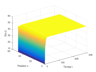
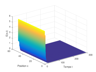
Figure 1: Evolution of $S$ and $E$ of model (6) for $x$ fixed and with the parameters described in Section 4. In this case, $R_{0}=0.8264<1$.

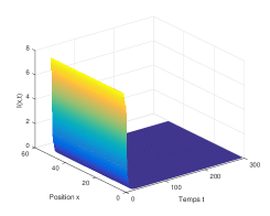
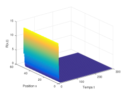
Figure 2: Evolution of $I$ and $R$ of model (6) for $x$ fixed and with the parameters described in Section 4. In this case, $R_{0}=0.8264<1$.

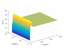
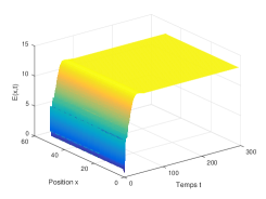
Figure 3: Evolution of $S$ and $E$ of model (6) with the parameters described in Section 4, excepting $\mu=0.03$ and $\alpha=0.2$. In this case, $R_{0}=11.3669>1$.

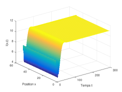
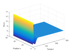
Figure 4: Evolution of $I$ and $R$ of model (6) with the parameters described in Section 4, excepting $\mu=0.03$ and $\alpha=0.2$. In this case, $R_{0}=11.3669>1$.

From Figures 1 and 2, we note that the solution $(S(t),E(t),I(t),R(t))$ of system (6) converges to the free disease equilibrium $E_{0}=\left(50,0,0,0\right)$. In other words, $E_{0}$ is globally asymptotically stable. From a biological point of view, if $R_{0}\leq 1$, then the infection can be eradicated from the population. In addition, from Figures 3 and 4, we can draw the following conclusion: for $R_{0}>1$, the solution $(S(t),E(t),I(t),R(t))$ of model (6) converges to the endemic equilibrium $E^{*}$. Thus, the unique endemic equilibrium is globally asymptotically stable, which biologically means that the infection persists but is controlled.

It should be noted that our numerical simulations can be performed, without any difficulty, for dimension two in space.

5 Concluding remarks

We have studied the qualitative behavior of solutions of a reaction-diffusion system with distributed delay and a general nonlinear incidence function. We have shown that the model exhibits two equilibria: a disease-free equilibrium $E_{0}$ and an endemic equilibrium $E^{*}$. Under some assumptions on the incidence function, we have shown that the global dynamics of the model is completely determined by the basic reproduction number $R_{0}$. More precisely, we have proved that $R_{0}$ serves as a threshold parameter for the persistence and extinction of the disease. Since the coefficients of the system (1) are all constants, we took the advantages of the method of Lyapunov functions to obtain the global dynamics of the considered model, showing that the disease free equilibrium state is globally asymptotically stable for $R_{0}\leq 1$. When $R_{0}>1$, then we proved that there is a unique disease endemic equilibrium, which is globally asymptotically stable. Epidemiologically, this means that the disease will die out or will persist in the population depending on the values of the parameters of the model.

References

• [1]
• [2] M. Samsuzzoha, M. Singh, D. Lucy, Numerical study of an influenza epidemic model with diffusion, Applied Mathematics and Computation 217 (7) (2010) 3461–3479.
• [3] M. Samsuzzoha, M. Singh, D. Lucy, Numerical study of a diffusive epidemic model of influenza with variable transmission coefficient, Applied Mathematical Modelling 35 (12) (2011) 5507–5523.
• [4] Z. Bai, R. Peng, X. Q. Zhao, A reaction-diffusion malaria model with seasonality and incubation period, Journal of Mathematical Biology 77 (1) (2018) 201–228.
• [5] M. Banerjee, V. Volpert, Spatio-temporal pattern formation in Rosenzweig–MacArthur model: Effect of nonlocal interactions, Ecological Complexity 30 (2017) 2–10, Dynamical Systems In Biomathematics. doi:10.1016/j.ecocom.2016.12.002.
• [6] T. W. Hwang, F. B. Wang, Dynamics of a dengue fever transmission model with crowding effect in human population and spatial variation, Discrete & Continuous Dynamical Systems – B 18 (2013) 147–161.
• [7] Y. Lou, X. Q. Zhao, A reaction-diffusion malaria model with incubation period in the vector population, Journal of Mathematical Biology 62 (4) (2011) 543–568.
• [8] S. Wang, Threshold dynamics of an SIR epidemic model with nonlinear incidence rate and non-local delay effect, Wuhan University Journal of Natural Sciences 23 (6) (2018) 503–513.
• [9] Z.-t. Xu, D.-x. Chen, An SIS epidemic model with diffusion, Appl. Math. J. Chinese Univ. Ser. B 32 (2) (2017) 127–146. doi:10.1007/s11766-017-3460-1.
• [10] N. Ahmed, Z. Wei, D. Baleanu, M. Rafiq, M. A. Rehman, Spatio-temporal numerical modeling of reaction-diffusion measles epidemic system, Chaos: An Interdisciplinary Journal of Nonlinear Science 29 (10) (2019) 103101.
• [11] T. Kuniya, J. Wang, Lyapunov functions and global stability for a spatially diffusive SIR epidemic model, Applicable Analysis 96 (11) (2017) 1935–1960.
• [12] K. I. Kim, Z. Lin, Q. Zhang, An SIR epidemic model with free boundary, Nonlinear Analysis: Real World Applications 14 (5) (2013) 1992–2001.
• [13] V. Capasso, G. Serio, A generalization of the Kermack-McKendrick deterministic epidemic model, Mathematical Biosciences 42 (1) (1978) 43–61.
• [14] A. Elazzouzi, A. Lamrani Alaoui, M. Tilioua, D. F. M. Torres, Analysis of a SIRI epidemic model with distributed delay and relapse, Statistics, Optimization and Information Computing 7 (2019) 545–557. arXiv:1812.09626
• [15] Y. Enatsu, Lyapunov functional techniques on the global stability of equilibria of SIS epidemic models with delays, Kyoto Univ. Res. Inf. Repository 1792 (2012) 118–130.
• [16] A. Kaddar, Stability analysis in a delayed SIR epidemic model with a saturated incidence rate, Nonlinear Anal. Model. Control 15 (3) (2010) 299–306.
• [17] A. Korobeinikov, P. K. Maini, A Lyapunov function and global properties for SIR and SEIR epidemiological models with nonlinear incidence, Math. Biosci. Eng. 1 (1) (2004) 57–60.
• [18] A. Lahrouz, L. Omari, D. Kiouach, A. Belmaâti, Complete global stability for an SIRS epidemic model with generalized non-linear incidence and vaccination, Appl. Math. Comput. 218 (11) (2012) 6519–6525.
• [19] J. J. Wang, J. Z. Zhang, Z. Jin, Analysis of an SIR model with bilinear incidence rate, Nonlinear Analysis: Real World Applications 11 (4) (2010) 2390–2402.
• [20] A. B. Gumel, S. M. Moghadas, A qualitative study of a vaccination model with non-linear incidence, Applied Mathematics and Computation 143 (2003) 409–419.
• [21] J. Li, G. Q. Sun, Z. Jin, Pattern formation of an epidemic model with time delay, Physica A: Statistical Mechanics and its Applications 403 (2014) 100–109.
• [22] S. Ruan, W. Wang, Dynamical behavior of an epidemic model with a nonlinear incidence rate, Journal of Differential Equations 188 (2003) 135–163.
• [23] A. Elazzouzi, A. Lamrani Alaoui, M. Tilioua, A. Tridane, Global stability analysis for a generalized delayed SIR model with vaccination and treatment, Advances in Difference Equations 532 (2019) (2019).
• [24] J. Yang, S. Liang, Y. Zhang, Travelling waves of a delayed SIR epidemic model with nonlinear incidence rate and spatial diffusion, PLOS ONE 6 (2011) 1–14.
• [25] W. Xia, S. Kundu, S. Maitra, Dynamics of a delayed SEIQ epidemic model, Advances in Difference Equations 2018 (2018) 336.
• [26] C. C. McCluskey, Y. Yang, Global stability of a diffusive virus dynamics model with general incidence function and time delay, Nonlinear Anal. Real World Appl. 25 (2015) 64–78. doi:10.1016/j.nonrwa.2015.03.002.
• [27] H. Yang, J. Wei, Dynamics of spatially heterogeneous viral model with time delay, Communications on Pure & Applied Analysis 19 (2020) 85–102.
• [28] C. C. McCluskey, Global stability of an SIR epidemic model with delay and general nonlinear incidence, Math. Biosci. Eng. 7 (4) (2010) 837–850. doi:10.3934/mbe.2010.7.837.
• [29] J. K. Hale, Theory of functional differential equations, Part of the Applied Mathematical Sciences book series (AMS, volume 3), Springer-Verlag (1977).
• [30] J. K. Hale, Ordinary Differential Equations, Krieger publishing company Malabar, Florida, 1980.
• [31] D. Henry, Geometric Theory of Semilinear Parabolic Equations, Springer, New York, 1981.