Observational appearance of Kaluza-Klein black holes
Abstract
The optical properties of rotating black holes in Kaluza-Klein theory described by the total mass, spin, and electric and magnetic charges are investigated in detail. Using a developed general relativistic ray-tracing code to calculate the motion of photons, shadows of Kaluza-Klein black holes are generated. The properties of the shadow and the light deflection angle around these black holes are also studied in order to put constraints on the parameters of Kaluza-Klein black holes using M87* shadow observations. The possibility of imposing constraints on Kaluza-Klein black holes using shadow observations is investigated. Moreover, we find that small charges (electric and magnetic) of the black hole can meet these constraints. We conclude that with the current precision of the M87* black hole shadow image observation by the EHT collaboration, the shadow observations of Kaluza-Klein black holes are indistinguishable from that of the Kerr black hole. Much better observational accuracy than the current capabilities of the EHT collaboration are required in order to place verified constraints on the parameters of modified theories of gravity in the strong field regime.
I Introduction
The existing and rapidly growing experimental and observational data on astrophysical black hole candidates do not yet substantially support the idea that they should be well described by the Kerr spacetime metric. There are still open windows for consideration of other solutions within general relativity and/or modified theories of gravity Bambi (2017); Berti et al. (2015); Cardoso and Gualtieri (2016); Cardoso and Pani (2017); Krawczynski (2012, 2018); Yagi and Stein (2016); Bambi et al. (2016); Yunes and Siemens (2013); Tripathi et al. (2021). Thus, one needs to think of how to test gravity theories through different observational and experimental data in both the weak and strong field regimes.
Existing observational and experimental tests of gravity theories (see, e.g. Gravity Collaboration et al. (2018)) cannot determine the metric coefficients of the Kerr spacetime with high accuracy. There is still hope that quickly developing technologies will lead to improved accuracy and help determine the physical characteristics of Kerr black holes with high confidence. The first ever image or so-called shadow of the supermassive black hole (SMBH) at the center of the galaxy M87 has been captured using the VLBI (Very Long Baseline Interferometry) technique by the Event Horizon Telescope (EHT) collaboration Akiyama et al. (2019a, b). The obtained shadow of the SMBH M87* is consistent with expectations for the Kerr black hole shadow as predicted by general relativity. However, there is still a degeneracy problem since other axially-symmetric solutions within general relativity or modified theories of gravity can, in principle, mimic the Kerr spacetime parameters Carballo-Rubio et al. (2018); Abdikamalov et al. (2019). Several papers have also shown that weakly naked singularities also mimic black holes very well Virbhadra and Ellis (2002); Virbhadra and Keeton (2008).
Particularly the shadows of axially-symmetric Kerr-like black hole solutions have been investigated and the deviation from the Kerr black hole has been analyzed Takahashi (2005); Bambi and Freese (2009); Hioki and Maeda (2009); Amarilla et al. (2010); Bambi and Yoshida (2010); Amarilla and Eiroa (2012, 2013); Abdujabbarov et al. (2013); Atamurotov et al. (2013a); Wei and Liu (2013); Atamurotov et al. (2013b); Bambi (2015); Ghasemi-Nodehi et al. (2015); Cunha et al. (2015); Boshkayev et al. (2016); Quevedo (2011); Javed et al. (2019); Övgün et al. (2019); Övgün (2019); Johannsen and Psaltis (2011); Younsi et al. (2016); Ayzenberg and Yunes (2018). Detailed studies of the observable quantities of the black hole shadow in various theories of gravity can be found in Abdujabbarov et al. (2015); Atamurotov et al. (2015); Ohgami and Sakai (2015); Grenzebach et al. (2015); Mureika and Varieschi (2017); Abdujabbarov et al. (2017, 2016a, 2016b); Mizuno et al. (2018); Shaikh et al. (2018); Bisnovatyi-Kogan and Tsupko (2017); Perlick and Tsupko (2017); Schee and Stuchlík (2015, 2009a); Stuchlík and Schee (2014); Schee and Stuchlík (2009b); Stuchlík and Schee (2010); Mishra et al. (2019); Eiroa and Sendra (2018); Giddings (2019); Ayzenberg and Yunes (2018); Perlick and Tsupko (2022); Perlick et al. (2018); Solanki and Perlick (2022); Frost and Perlick (2021); Manojlovic et al. (2020); Olmo et al. (2023); Vincent et al. (2022).
Among the numerous alternative theories of gravity, the one proposed by Kaluza and Klein at the beginning of the 20th century has its own interesting features. Being proposed as a classical field theory, it can also be interpreted in the frameworks of quantum mechanics and string theory. The Kaluza-Klein theory is a five-dimensional theory and includes gravitational, electromagnetic, and scalar fields. The effects of a compact fifth dimension have been searched for in experiments at the Large Hadron Collider CMS Collaboration (2011) without any success up to now. Astrophysical tests of the Kaluza-Klein theory have been performed using analysis of the equations of motion and its application to galactic motion/rotation curves Wesson and Ponce de Leon (1995). Particularly, the shadow of one of the black hole solutions of the theory has been studied in Amarilla and Eiroa (2013). On the other hand, future modifications and improvements of gravitational wave observations may give some constraints on the theory Cardoso et al. (2019); Andriot and Lucena Gómez (2017); Abbott et al. (2016). In Azreg-Aïnou et al. (2020); Zhu et al. (2020), the authors have studied the effects of the Kaluza-Klein theory on the precession of a gyroscope and possible tests using X-ray spectroscopy. Here we plan to extend our previous studies by considering the shadow cast by a black hole within the Kaluza-Klein theory.
Several solutions have been obtained within the Kaluza-Klein theory describing compact objects and particularly black holes Horowitz and Wiseman (2011). In Refs. Dobiasch and Maison (1982); Chodos and Detweiler (1982); Gibbons and Wiltshire (1986) one may find different spherically-symmetric solutions of the theory. The axially-symmetric solutions of the Kaluza-Klein theory have been obtained in Refs. Larsen (2000); Rasheed (1995); Matos and Mora (1997) for the cases of four- and five-dimensional spacetimes. The black hole solution with squashed horizon has been studied in Ishihara and Matsuno (2006); Wang (2006). The solutions for black holes in higher dimensional spacetimes have been obtained in Park (1998).
In this paper, we study the optical properties of rotating black holes in Kaluza-Klein theory described by the four parameters of total mass, spin, electric and magnetic charges. The paper is organized as follows: The spacetime metric of a Kaluza-Klein black hole is presented and its properties are described in Sect. II. Sect. III is devoted to the development of the ray-tracing code for studying the photon motion and obtaining the black hole shadow. In Sect. IV, the shadow of the Kaluza-Klein black hole is explored and, in addition, the light deflection angle for gravitational lensing by the black hole is studied. Finally, we summarize our main results in Sect. V.
II Spacetime metric
For the spacetime metric, the notation developed in Azreg-Aïnou et al. (2020) will be used. In order to maintain consistency with our geometrized system of units, we adopt the convention of setting the speed of light, , to unity, i.e., . Additionally, the covariant derivatives represented by and the coordinate systems are used within the framework of the general metric ansatz for five-dimensional space-time. This ansatz encapsulates the spatial dimensions, , aligns with the time coordinate, , and designates the fifth or extra dimension, . There are three fields involved in the simplest Kaluza-Klein theory: gravity, the dilaton, and the gauge field. The canonical form of the action in the Einstein frame can be written as follows:
| (1) | ||||
where represents the determinant of the four-dimensional metric tensor, is the Ricci scalar, is a dilaton scalar field, is the gauge field, and is the gravitational constant. The metric in the Kaluza-Klein theory is given as
| (2) |
where
| (3) | ||||
and the one-forms are given by
| (4) | ||||
The physical mass , angular momentum , electric charge , and magnetic charge are included in the solution via four free parameters, , , , and , respectively. The relations are written as:
| (5) |
The four dimensional version of the metric in the Einstein frame is given by
| (6) |
where
| (7) | ||||
and . Here , , , and are the dimensionless parameters that are defined as , , , and . From Eq. 5, the free parameter can be related to the physical mass as
| (8) |
The Kaluza-Klein metric reduces to the Kerr metric when the electric and magnetic charges vanish, and the spin parameter equals the Kerr solution’s dimensionless spin . The spacetime has two horizons
| (9) |
which are obtained by solving . In terms of the dimensionless parameters Eq. 9 becomes
| (10) |
The Reissner-Nordstrom solution of general relativity is obtained by setting and . We recover the Kerr solution when . However, the Kerr-Newman solution is not recovered when the magnetic charge vanishes. For our analysis, we consider the case when , which is a black hole with electric and magnetic charges. Note that this case can only be considered as a toy-model, since macroscopic black holes have a negligible electric charge.
Next, we make sure that the spacetime does not possess any pathologies. The bounds on the free parameters are obtained by preserving the metric structure everywhere outside the horizon. First, from the definitions of and in Eq. 5, we get the following constraints: , , or , . Plugging these into Eq. 10, we come to the bound on :
| (11) |
The upper bound of () can be obtained by using Eqs. 10-11 as
| (12) |
III Ray-tracing code for photons
The photon sphere of a black hole spacetime separates geodesics falling into the event horizon from those escaping to spatial infinity Claudel et al. (2001). We observe the photon sphere in the form of the black hole shadow. In the case of generic spacetimes, we cannot solve the null-geodesic equations analytically and we have to solve the photon motion numerically in order to calculate the shadow. In the Kerr spacetime, the photon sphere is described by an analytical solution that is used to calculate the shadow. The Kaluza-Klein black hole metric we are studying is not separable and, therefore, the shadow will be calculated numerically by applying a general relativistic ray-tracing code, which will be described below.
The ray-tracing code we apply calculates photon trajectories near the black hole and is based on the code used in Ayzenberg and Yunes (2018); Gott et al. (2019); Abdikamalov et al. (2019), which was first described in Psaltis and Johannsen (2012). To obtain the equations that represent - and - component of the photon position, we exploit the property of all stationary and axisymmetric spacetimes, namely, that a test particle’s four momentum is related to the specific energy and the -component of the specific angular momentum as and . These relations lead to two first-order differential equations
| (13) |
| (14) |
where denotes the normalized affine parameter and is the impact parameter.
The - and -components of the photon position are obtained by solving the second-order geodesic equations for a generic axisymmetric metric
| (15) | ||||
| (16) | ||||
where the Christoffel symbols of the metric are given by .
We set the reference frame and coordinate system in such a way that the black hole is at the origin and -axis coincides with the axis of the spin angular momentum. In the code we set the physical mass as , since the shape of the black hole shadow does not depend on the physical mass , which only affects the size of the shadow. In the calculations, the distance, azimuthal angle, and polar angle of the observing screen are set to , , and , respectively. The relations and link the polar coordinates and used on the screen and the celestial coordinates on the observer’s sky.
The system of equations (15)-(16) are evolved backwards in time, since only the final positions and momenta of the photons are known. Each photon originates with some initial coordinates on the screen having a four-momentum perpendicular to the screen. The latter condition is necessary for modeling the position of the screen located very far from the source, since photons hitting the screen at spatial infinity would move perpendicular to the screen at a distance of .
Each photon’s initial position and four-momentum in the Boyer-Lindquist coordinates of the black hole spacetime are expressed as Bambi (2017)
| (17) |
| (18) |
| (19) |
and
| (20) |
| (21) |
| (22) |
| (23) |
We can find the component from the fact that the norm of the photon four-momentum is zero. The conserved quantity required in Eqs. (13) and (14) can be calculated from the initial conditions.
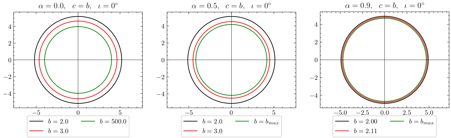
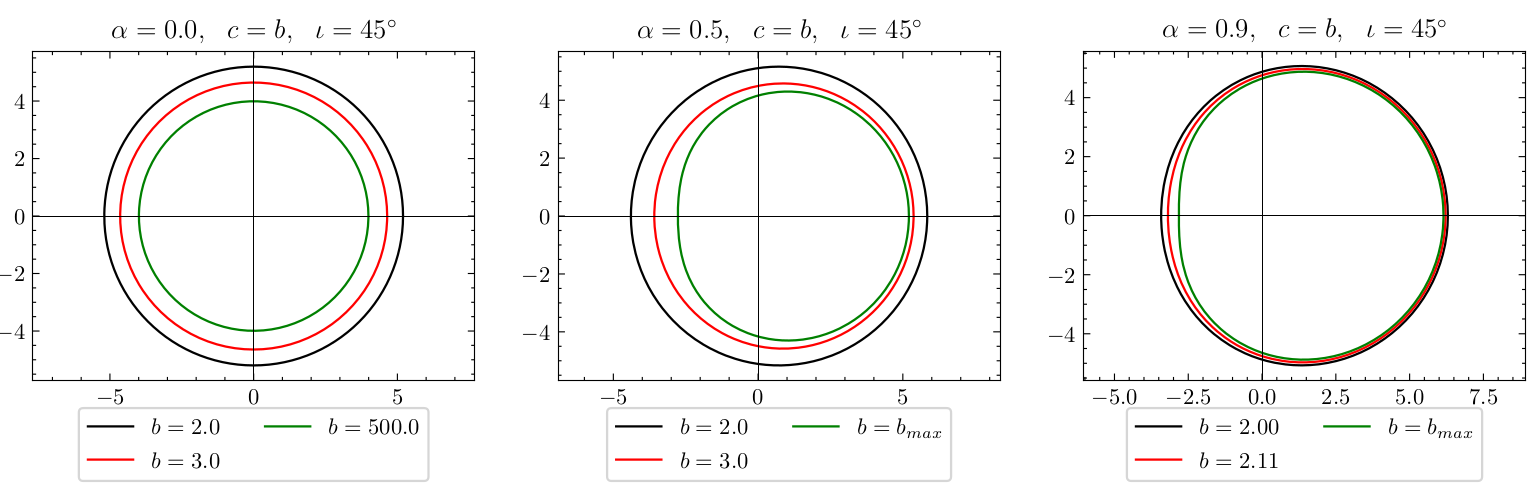
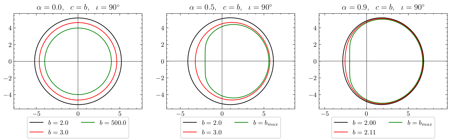
The initial conditions on the screen are sampled by the code in the following way. The location of the shadow boundary separating photons falling into the horizon from those fleeing into spatial infinity is searched in the range for each in the range and in increments . Photons intersecting , with , are considered captured in the horizon, while all other photons reach , hence escaping to spatial infinity. The accurate value of that represents the shadow boundary for current is determined by zooming in the boundary to an accuracy . This methodology can accurately calculate the black hole shadow more efficiently than fine sampling the entire screen. Fig. 1 shows the shadow silhouettes calculated using the ray-tracing code for and several values of the deformation parameter at an inclination angle . Fig. 2 and Fig. 3 illustrate the same images calculated at inclination angles and . When , the shadow images are circles with different sizes affected by and . For , the barycenter of the images moves away from the center and the distortion of the shadow from a circle increases as spin increases. Also, the same effects are achieved by increasing for fixed .
IV Shadow of Kaluza-Klein black holes
In this section, we will study the apparent shape of the Kaluza-Klein black hole shadow. We consider the celestial coordinates and (see Vázquez and Esteban (2004); Abdujabbarov et al. (2016b) for reference) defined as,
| (24) | |||||
| (25) |
where denotes the distance between the observer and black hole and is the inclination angle between the black hole spin axis and the observer’s line of sight. We will apply the coordinate independent formalism used in Ayzenberg and Yunes (2018) to describe the relationship between the shape of the shadow and the deformation parameter. The horizontal displacement from the center of the image , the average radius of the sphere , and the asymmetry parameter parametrize the shape of the shadow. We will get similar results with any other chosen parametrizations (see e.g. Tsukamoto et al. (2014); Abdujabbarov et al. (2015)). The horizontal displacement registers the shift of the shadow center from the center of the black hole, and it is defined as
| (26) |
where and represent the maximum and
minimum horizontal coordinates of the image on the observing screen, respectively. We can safely ignore the vertical displacement of the image, since the spacetime in which we are working is axisymmetric. The average radius defines the average distance between the boundary and the center of the shadow, which is defined by
| (27) |
where and . The asymmetry parameter characterizes the distortion of the shadow from a circle, and it is defined by
| (28) |
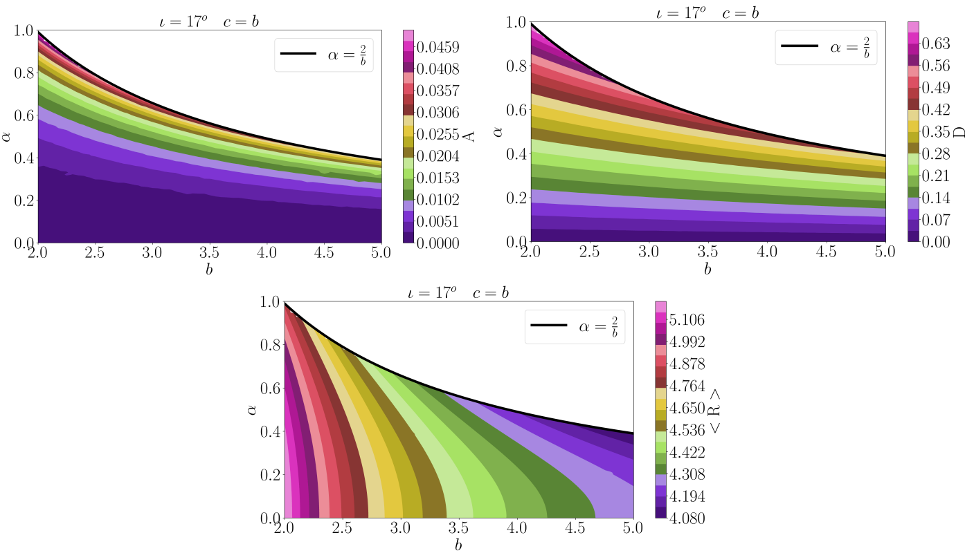
Fig. 4 shows the density plot of the shadow parametrizations: asymmetry parameter (top left panel), horizontal displacement (top right panel) and average radius (bottom panel). The black solid curves mark the upper boundary of the parameter (). By varying , the same values of the asymmetry parameter and the horizontal displacement can be obtained for different values of . As we can see, is the main parameter that affects the values of and , and is the main parameter that affects . Additionally, the influence of the parameter on both and manifests distinct behaviors. In the former case, exhibits a power-law relationship, while in the latter case, the impact is approximately linear.
IV.1 Deflection angle
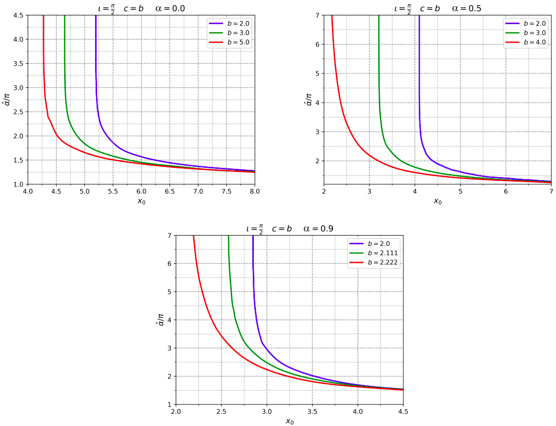
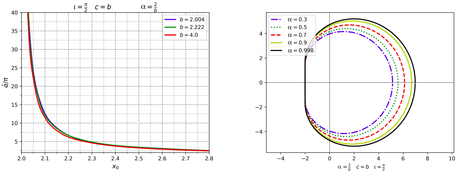
Here we calculate the deflection angle of photons that pass near the black hole using the modified version of the ray-tracing code described above. The calculation algorithms are similar to those discussed in Sec. III. We restrict the entire photon trajectories to the equatorial plane of the Kaluza-Klein black hole. We initialize photons on the screen with certain celestial coordinates . Setting , and in Eqs. 17-23 lead to , with non-zero , , so we obtain the photon trajectories lying in the equatorial plane. is chosen in such a way that photons with the impact parameter approach the photon ring of the black hole at the minimum coordinate difference without crossing it. The deflection angle from a straight line is calculated by capturing the initial and final positions of the photon. Fig. 5 illustrates the calculated values of the deflection angle as a function of photons with impact parameter for . Increasing shifts the impact parameter towards lower values. This can be explained by an increase of the horizontal displacement and a distortion from a circle. Fig. 6 shows the deflection angles and shadow images for several values of the spin parameter with maximum allowed . We can see that the deflection angles are nearly the same. Also, from the corresponding shadow images, the horizontal displacement and the distortion take similar values.
IV.2 A simple constraint of the Kaluza-Klein black hole parameters using the M87* results
Now we plan to study whether one can place constraints on the parameters of a Kaluza-Klein BH using the M87* black hole shadow observations. We follow the precept of Akiyama et al. (2019a) that EHT observations are related to the shadow of a rotating Kerr BH. Based on the results from the shadow of M87* BH observations, we constrain the parameter (assuming ) and the spin of the Kaluza-Klein black hole using the average radius (Eq. 27) and the asymmetry parameter (Eq. 28) of the BH shadow. Note that this approach is a simplification of the correct analysis, in which the calculated shadows should be convolved with the response of the instrument, followed by a final comparison of the output data with EHT data.
According to observations made by the EHT collaboration, the angular size of the observed shadow is , and a deviation from circularity is less than
Furthermore, we take the standard values for the distance to to be and the total mass of the object to be . Taking into account the accepted values of physical quantities, the average radius of the BH shadow is evaluated as
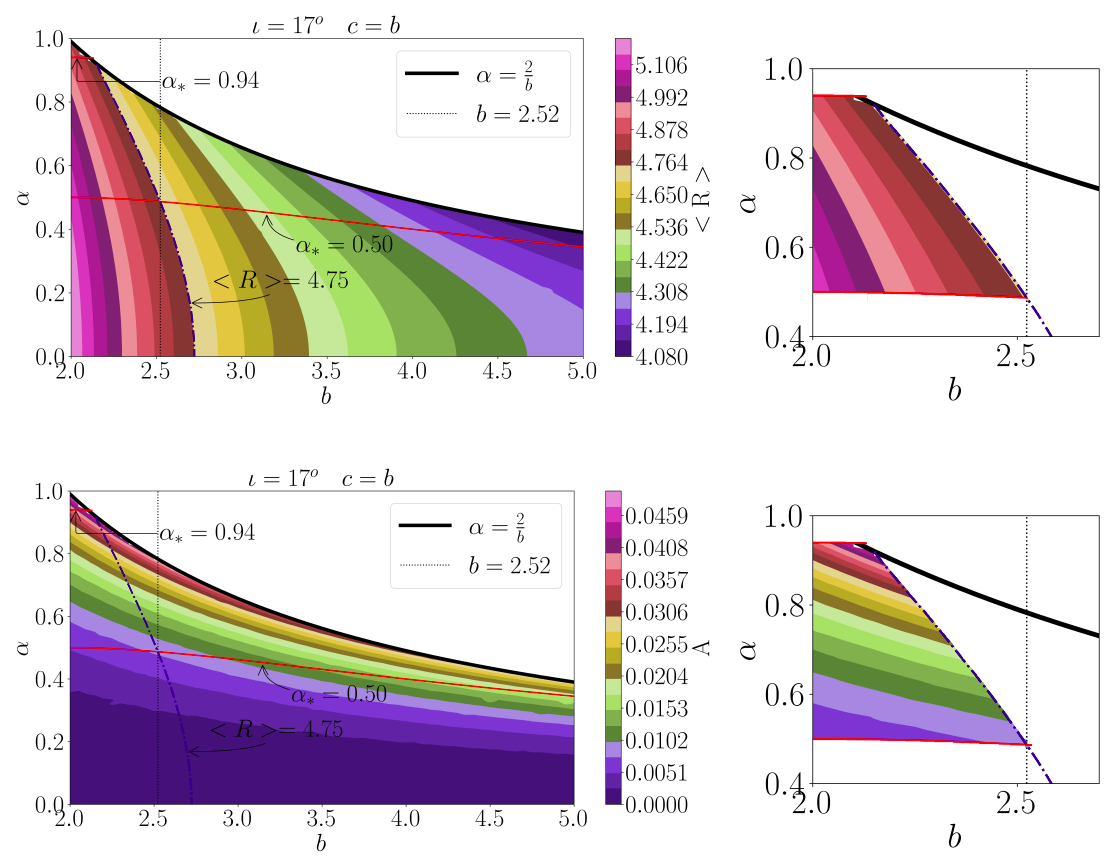
In Fig. 7, the average radius and the asymmetry parameter of the BH shadow are shown for different values of the parameters and . Here, we have taken the inclination angle to be , which the observed M87 jet axis makes with respect to the line of sight. Moreover, according to the observations by EHT collaboration, the BH spin lies within the range , where (here is the angular momentum of BH).
The maximum value for the BH shadow radius is . For the Kaluza-Klein black hole, the greatest value is the average radius of the shadow , so we have a limit on the size of the BH shadow from below, i.e. as . Given the spin range and using Eq. 5, we plot the curves and (red lines in Fig. 7) as well as the line . As a result, we obtain the largest possible upper bound for the parameter, , where . With such a constraint, the asymmetry parameter of the BH shadow is always less than 0.05.
IV.3 Images of a Kaluza-Klein black hole surrounded with thin accretion disk
In this subsection we explore the Novikov-Thorne model of a thin accretion disk around a Kaluza-Klein black hole. To obtain an image of the accretion disk around the black hole, we use the ray-tracing code developed and presented in Sect. III. A pivotal component in the creation of the image of a thin disk involves the radiation flux emission profile. When considering a massive test particle that orbits the metric in the Kaluza-Klein theory on a circular orbit within the equatorial plane (), the effective potential for the particle takes the form:
| (29) |
The specific energy and the specific angular momentum can be expressed as:
| (30) |
| (31) |
where is the angular velocity
| (32) |
The inner edge of the thin accretion disk is determined by the innermost stable circular orbit (ISCO). The ISCO’s location is derived from the following conditions:
| (33) |
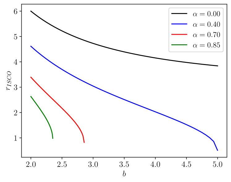
Fig. 8 illustrates the radius of the innermost stable circular orbit () as a function of the parameter for different values of the parameter based on the solution derived from Eq. 33. As evident from the figure, the value of decreases as the parameters and increase.
By selecting initial conditions for photons as the photons cross the accretion disk, one can calculate the energy flux for them as
| (34) |
where is the mass accretion rate and is the radius of the inner edge of the accretion disk, which is equivalently equal to .
The photon flux as detected by a distant observer is
| (35) |
where is the redshift factor which comprises the effects of both gravitational redshift and Doppler shift
| (36) |
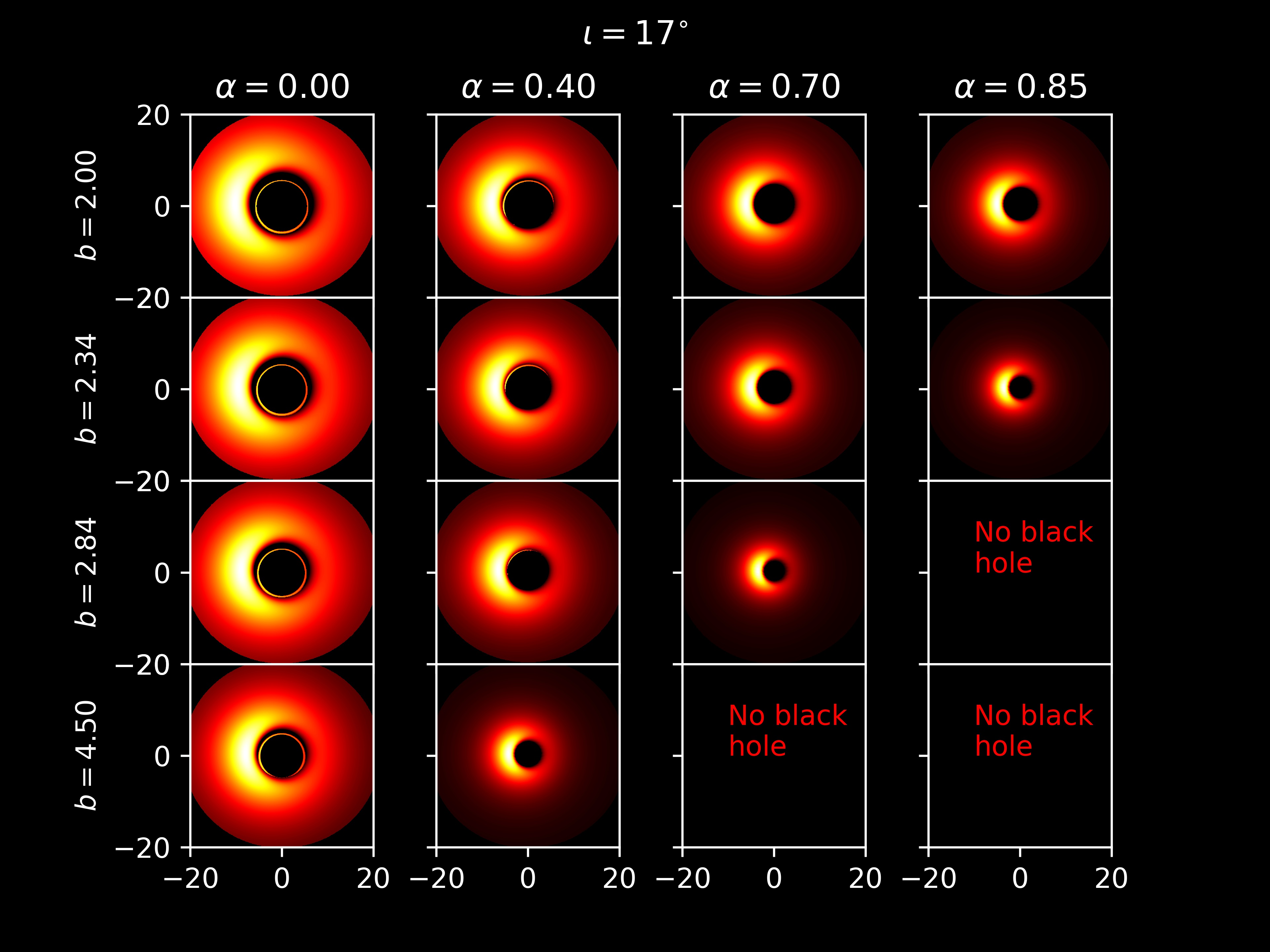
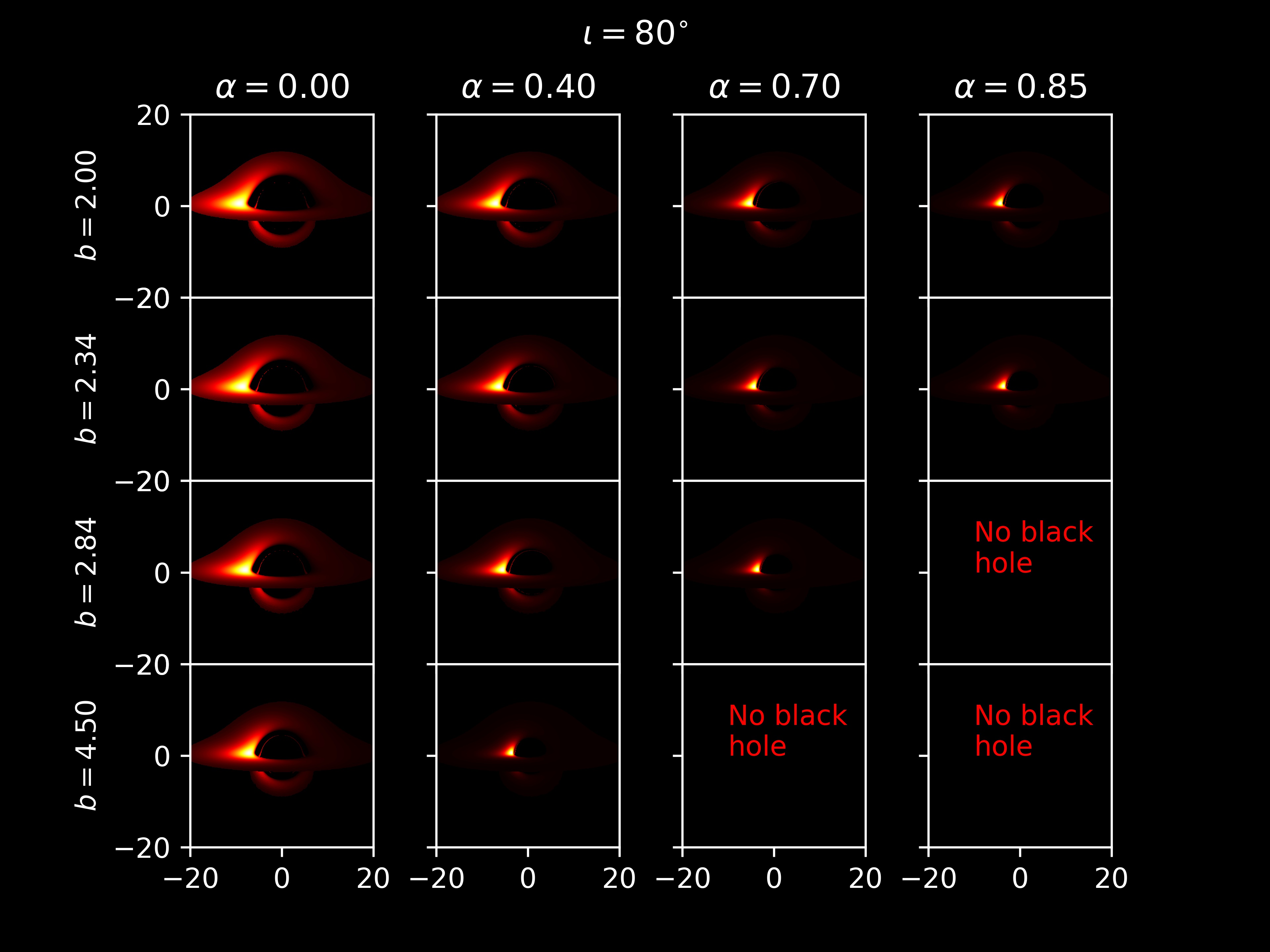
Figure 9 illustrates images of the accretion disk for the case when the inclination angle and and for the different values of BH parameters and .
One can observe that with an increase of the values of the parameters and , the photon ring starts to disappear due to the fact that the BH image with the accretion disk completely or partially overlaps the photon ring. As decreases with increasing parameters and , the photon ring begins to overlap with the inner edge of the disk. We hope to compare our results with images of thin accretion disks from future X-ray interferometric missions Uttley et al. (2021).
V Conclusions
Our results on the optical properties of a rotating black hole in Kaluza-Klein theory described by the parameters of total mass, spin, electric and magnetic charges can be summarized as follows:
-
•
The photon motion in the close environment of a rotating black hole in Kaluza-Klein theory is extensively explored. The photon sphere produced by the photons at the last stable orbits shifts towards the central object under the effect of magnetic and electric charges.
-
•
For the gravitational lensing in strong field regime, the deflection angle of photons that pass near the boundary of the shadow of the rotating Kaluza-Klein black hole are obtained numerically using the developed ray-tracing code for the photon motion. The obtained results indicate that the deflection angle of photons decrease with the increase of electric and magnetic charges.
-
•
Numerous synthetic BH shadows are generated and their properties, together with the light deflection angle, around a Kaluza-Klein black hole are studied. Then synthetic images of Kaluza-Klein black holes are compared with the EHT observations of the M87* SMBH shadow in order to put constraints on the parameters of a Kaluza-Klein BH. The constraint on the upper limit of the dimensionless magnetic (electric) charge of the BH is obtained as . The upper limit of the asymmetry parameter of the BH shadow is obtained as . From the number of BH images generated, the cases and are found to most closely match that of the M87* images observed by the EHT collaboration.
We can conclude that, based on the current precision of the M87* black hole shadow image observation by the EHT collaboration, the shadow observations of Kaluza-Klein BHs are almost indistinguishable from that of Kerr BHs. Much better observational accuracy than the current capabilities of the EHT collaboration are required in order to place verified constraints on the parameters of modified theories of gravity in the strong field regime. In the future, with improved measurements from the EHT on , it is likely that the bound on will become more stringent.
acknowledgements
This work was supported in part by Grants F-FA-2021-432, F-FA-2021-510, and MRB-2021-527 of the Uzbekistan Ministry for Innovative Development and by the Abdus Salam International Centre for Theoretical Physics under the Grant No. OEA-NT-01. D.A. was supported by the Teach@Tübingen and Research@Tübingen Fellowships. T.M. acknowledges also the support from the China Scholarship Council (CSC), Grant No. 2022GXZ005433.
References
- Bambi (2017) C. Bambi, Reviews of Modern Physics 89, 025001 (2017).
- Berti et al. (2015) E. Berti, E. Barausse, V. Cardoso, L. Gualtieri, P. Pani, U. Sperhake, L. C. Stein, N. Wex, K. Yagi, T. Baker, C. P. Burgess, F. S. Coelho, D. Doneva, A. De Felice, P. G. Ferreira, P. C. C. Freire, J. Healy, C. Herdeiro, M. Horbatsch, B. Kleihaus, A. Klein, K. Kokkotas, J. Kunz, P. Laguna, R. N. Lang, T. G. F. Li, T. Littenberg, A. Matas, S. Mirshekari, H. Okawa, E. Radu, R. O’Shaughnessy, B. S. Sathyaprakash, C. Van Den Broeck, H. A. Winther, H. Witek, M. Emad Aghili, J. Alsing, B. Bolen, L. Bombelli, S. Caudill, L. Chen, J. C. Degollado, R. Fujita, C. Gao, D. Gerosa, S. Kamali, H. O. Silva, J. G. Rosa, L. Sadeghian, M. Sampaio, H. Sotani, and M. Zilhao, Classical and Quantum Gravity 32, 243001 (2015), arXiv:1501.07274 [gr-qc] .
- Cardoso and Gualtieri (2016) V. Cardoso and L. Gualtieri, Classical and Quantum Gravity 33, 174001 (2016), arXiv:1607.03133 [gr-qc] .
- Cardoso and Pani (2017) V. Cardoso and P. Pani, Nature Astronomy 1, 586 (2017), arXiv:1707.03021 [gr-qc] .
- Krawczynski (2012) H. Krawczynski, Astrophys J. 754, 133 (2012), arXiv:1205.7063 [gr-qc] .
- Krawczynski (2018) H. Krawczynski, General Relativity and Gravitation 50, 100 (2018), arXiv:1806.10347 [astro-ph.HE] .
- Yagi and Stein (2016) K. Yagi and L. C. Stein, Classical and Quantum Gravity 33, 054001 (2016), arXiv:1602.02413 [gr-qc] .
- Bambi et al. (2016) C. Bambi, J. Jiang, and J. F. Steiner, Classical and Quantum Gravity 33, 064001 (2016), arXiv:1511.07587 [gr-qc] .
- Yunes and Siemens (2013) N. Yunes and X. Siemens, Living Reviews in Relativity 16, 9 (2013), arXiv:1304.3473 [gr-qc] .
- Tripathi et al. (2021) A. Tripathi, Y. Zhang, A. B. Abdikamalov, D. Ayzenberg, C. Bambi, J. Jiang, H. Liu, and M. Zhou, Astrophys. J. 913, 79 (2021), arXiv:2012.10669 [astro-ph.HE] .
- Gravity Collaboration et al. (2018) Gravity Collaboration, R. Abuter, A. Amorim, N. Anugu, M. Bauböck, M. Benisty, J. P. Berger, N. Blind, H. Bonnet, W. Brandner, A. Buron, C. Collin, F. Chapron, Y. Clénet, V. Coudé Du Foresto, P. T. de Zeeuw, C. Deen, F. Delplancke-Ströbele, R. Dembet, J. Dexter, G. Duvert, A. Eckart, F. Eisenhauer, G. Finger, N. M. Förster Schreiber, P. Fédou, P. Garcia, R. Garcia Lopez, F. Gao, E. Gendron, R. Genzel, S. Gillessen, P. Gordo, M. Habibi, X. Haubois, M. Haug, F. Haußmann, T. Henning, S. Hippler, M. Horrobin, Z. Hubert, N. Hubin, A. Jimenez Rosales, L. Jochum, K. Jocou, A. Kaufer, S. Kellner, S. Kendrew, P. Kervella, Y. Kok, M. Kulas, S. Lacour, V. Lapeyrère, B. Lazareff, J.-B. Le Bouquin, P. Léna, M. Lippa, R. Lenzen, A. Mérand, E. Müler, U. Neumann, T. Ott, L. Palanca, T. Paumard, L. Pasquini, K. Perraut, G. Perrin, O. Pfuhl, P. M. Plewa, S. Rabien, A. Ramírez, J. Ramos, C. Rau, G. Rodríguez-Coira, R.-R. Rohloff, G. Rousset, J. Sanchez-Bermudez, S. Scheithauer, M. Schöller, N. Schuler, J. Spyromilio, O. Straub, C. Straubmeier, E. Sturm, L. J. Tacconi, K. R. W. Tristram, F. Vincent, S. von Fellenberg, I. Wank, I. Waisberg, F. Widmann, E. Wieprecht, M. Wiest, E. Wiezorrek, J. Woillez, S. Yazici, D. Ziegler, and G. Zins, Astronomy & Astrophysics 615, L15 (2018), arXiv:1807.09409 .
- Akiyama et al. (2019a) K. Akiyama et al. (Event Horizon Telescope), Astrophys. J. 875, L1 (2019a).
- Akiyama et al. (2019b) K. Akiyama et al. (Event Horizon Telescope), Astrophys. J. 875, L6 (2019b).
- Carballo-Rubio et al. (2018) R. Carballo-Rubio, F. Di Filippo, S. Liberati, and M. Visser, Phys. Rev. D 98, 124009 (2018), arXiv:1809.08238 [gr-qc] .
- Abdikamalov et al. (2019) A. B. Abdikamalov, A. A. Abdujabbarov, D. Ayzenberg, D. Malafarina, C. Bambi, and B. Ahmedov, Phys. Rev. D 100, 024014 (2019), arXiv:1904.06207 [gr-qc] .
- Virbhadra and Ellis (2002) K. S. Virbhadra and G. F. R. Ellis, Phys. Rev. D 65, 103004 (2002).
- Virbhadra and Keeton (2008) K. S. Virbhadra and C. R. Keeton, Phys. Rev. D 77, 124014 (2008).
- Takahashi (2005) R. Takahashi, Publications of the Astronomical Society of Japan 57, 273 (2005), astro-ph/0505316 .
- Bambi and Freese (2009) C. Bambi and K. Freese, Phys. Rev. D 79, 043002 (2009), arXiv:0812.1328 .
- Hioki and Maeda (2009) K. Hioki and K.-I. Maeda, Phys. Rev. D 80, 024042 (2009).
- Amarilla et al. (2010) L. Amarilla, E. F. Eiroa, and G. Giribet, Phys. Rev. D 81, 124045 (2010).
- Bambi and Yoshida (2010) C. Bambi and N. Yoshida, Classical and Quantum Gravity 27, 205006 (2010), arXiv:1004.3149 [gr-qc] .
- Amarilla and Eiroa (2012) L. Amarilla and E. F. Eiroa, Phys. Rev. D 85, 064019 (2012).
- Amarilla and Eiroa (2013) L. Amarilla and E. F. Eiroa, Phys. Rev. D 87, 044057 (2013).
- Abdujabbarov et al. (2013) A. Abdujabbarov, F. Atamurotov, Y. Kucukakca, B. Ahmedov, and U. Camci, Astrophys. Space Sci. 344, 429 (2013).
- Atamurotov et al. (2013a) F. Atamurotov, A. Abdujabbarov, and B. Ahmedov, Astrophys Space Sci 348, 179 (2013a).
- Wei and Liu (2013) S.-W. Wei and Y.-X. Liu, Journal of Cosmology and Astroparticles 11, 063 (2013), arXiv:1311.4251 [gr-qc] .
- Atamurotov et al. (2013b) F. Atamurotov, A. Abdujabbarov, and B. Ahmedov, Phys. Rev. D 88, 064004 (2013b).
- Bambi (2015) C. Bambi, arXiv e-prints , arXiv:1507.05257 (2015), arXiv:1507.05257 [gr-qc] .
- Ghasemi-Nodehi et al. (2015) M. Ghasemi-Nodehi, Z. Li, and C. Bambi, European Physical Journal C 75, 315 (2015), arXiv:1506.02627 [gr-qc] .
- Cunha et al. (2015) P. V. P. Cunha, C. A. R. Herdeiro, E. Radu, and H. F. Rúnarsson, Physical Review Letters 115, 211102 (2015), arXiv:1509.00021 [gr-qc] .
- Boshkayev et al. (2016) K. Boshkayev, E. Gasperin, A. C. Gutierrez-Pineres, H. Quevedo, and S. Toktarbay, Phys. Rev. D 93, 024024 (2016), arXiv:1509.03827 [gr-qc] .
- Quevedo (2011) H. Quevedo, International Journal of Modern Physics D 20, 1779 (2011), arXiv:1012.4030 [gr-qc] .
- Javed et al. (2019) W. Javed, R. Babar, and A. Övgün, Phys. Rev. D 99, 084012 (2019), arXiv:1903.11657 [gr-qc] .
- Övgün et al. (2019) A. Övgün, G. Gyulchev, and K. Jusufi, Annals of Physics 406, 152 (2019), arXiv:1806.03719 [gr-qc] .
- Övgün (2019) A. Övgün, Universe 5, 115 (2019), arXiv:1806.05549 [physics.gen-ph] .
- Johannsen and Psaltis (2011) T. Johannsen and D. Psaltis, Phys. Rev. D 83, 124015 (2011), arXiv:1105.3191 [gr-qc] .
- Younsi et al. (2016) Z. Younsi, A. Zhidenko, L. Rezzolla, R. Konoplya, and Y. Mizuno, Phys. Rev. D 94, 084025 (2016), arXiv:1607.05767 [gr-qc] .
- Ayzenberg and Yunes (2018) D. Ayzenberg and N. Yunes, Classical and Quantum Gravity 35, 235002 (2018), arXiv:1807.08422 [gr-qc] .
- Abdujabbarov et al. (2015) A. A. Abdujabbarov, L. Rezzolla, and B. J. Ahmedov, Mon. Not. R. Astron. Soc. 454, 2423 (2015), arXiv:1503.09054 [gr-qc] .
- Atamurotov et al. (2015) F. Atamurotov, B. Ahmedov, and A. Abdujabbarov, Phys. Rev. D 92, 084005 (2015), arXiv:1507.08131 [gr-qc] .
- Ohgami and Sakai (2015) T. Ohgami and N. Sakai, Phys. Rev. D 91, 124020 (2015).
- Grenzebach et al. (2015) A. Grenzebach, V. Perlick, and C. Lämmerzahl, International Journal of Modern Physics D 24, 1542024 (2015), arXiv:1503.03036 [gr-qc] .
- Mureika and Varieschi (2017) J. R. Mureika and G. U. Varieschi, Canadian Journal of Physics 95, 1299 (2017), arXiv:1611.00399 [gr-qc] .
- Abdujabbarov et al. (2017) A. Abdujabbarov, B. Toshmatov, Z. Stuchlík, and B. Ahmedov, International Journal of Modern Physics D 26, 1750051-239 (2017).
- Abdujabbarov et al. (2016a) A. Abdujabbarov, B. Juraev, B. Ahmedov, and Z. Stuchlík, Astrophys Space Sci 361, 226 (2016a).
- Abdujabbarov et al. (2016b) A. Abdujabbarov, M. Amir, B. Ahmedov, and S. G. Ghosh, Phys. Rev. D 93, 104004 (2016b), arXiv:1604.03809 [gr-qc] .
- Mizuno et al. (2018) Y. Mizuno, Z. Younsi, C. M. Fromm, O. Porth, M. De Laurentis, H. Olivares, H. Falcke, M. Kramer, and L. Rezzolla, Nature Astronomy (2018), 10.1038/s41550-018-0449-5, arXiv:1804.05812 .
- Shaikh et al. (2018) R. Shaikh, P. Kocherlakota, R. Narayan, and P. S. Joshi, ArXiv e-prints (2018), arXiv:1802.08060 [astro-ph.HE] .
- Bisnovatyi-Kogan and Tsupko (2017) G. Bisnovatyi-Kogan and O. Tsupko, Universe 3, 57 (2017).
- Perlick and Tsupko (2017) V. Perlick and O. Y. Tsupko, Phys. Rev. D 95, 104003 (2017), arXiv:1702.08768 [gr-qc] .
- Schee and Stuchlík (2015) J. Schee and Z. Stuchlík, JCAP 6, 048 (2015), arXiv:1501.00835 [astro-ph.HE] .
- Schee and Stuchlík (2009a) J. Schee and Z. Stuchlík, General Relativity and Gravitation 41, 1795 (2009a), arXiv:0812.3017 .
- Stuchlík and Schee (2014) Z. Stuchlík and J. Schee, Classical and Quantum Gravity 31, 195013 (2014), arXiv:1402.2891 [astro-ph.HE] .
- Schee and Stuchlík (2009b) J. Schee and Z. Stuchlík, International Journal of Modern Physics D 18, 983 (2009b), arXiv:0810.4445 .
- Stuchlík and Schee (2010) Z. Stuchlík and J. Schee, Classical and Quantum Gravity 27, 215017 (2010), arXiv:1101.3569 [gr-qc] .
- Mishra et al. (2019) A. K. Mishra, S. Chakraborty, and S. Sarkar, arXiv e-prints (2019), arXiv:1903.06376 [gr-qc] .
- Eiroa and Sendra (2018) E. F. Eiroa and C. M. Sendra, The European Physical Journal C 78, 91 (2018).
- Giddings (2019) S. B. Giddings, Universe 5, 201 (2019), arXiv:1904.05287 [gr-qc] .
- Perlick and Tsupko (2022) V. Perlick and O. Y. Tsupko, Physics Reports 947, 1 (2022).
- Perlick et al. (2018) V. Perlick, O. Y. Tsupko, and G. S. Bisnovatyi-Kogan, Phys. Rev. D 97, 104062 (2018).
- Solanki and Perlick (2022) J. Solanki and V. Perlick, Phys. Rev. D 105, 064056 (2022).
- Frost and Perlick (2021) T. C. Frost and V. Perlick, Classical and Quantum Gravity 38, 085016 (2021).
- Manojlovic et al. (2020) N. Manojlovic, V. Perlick, and R. Potting, Annals Phys. 422, 168303 (2020), arXiv:2006.09053 [math-ph] .
- Olmo et al. (2023) G. J. Olmo, J. L. Rosa, D. Rubiera-Garcia, and D. S.-C. Gómez, Classical and Quantum Gravity 40, 174002 (2023).
- Vincent et al. (2022) F. H. Vincent, S. E. Gralla, A. Lupsasca, and M. Wielgus, Astron. Astrophys. 667, A170 (2022), arXiv:2206.12066 [astro-ph.HE] .
- CMS Collaboration (2011) CMS Collaboration, Physics Letters B 697, 434 (2011), arXiv:1012.3375 [hep-ex] .
- Wesson and Ponce de Leon (1995) P. S. Wesson and J. Ponce de Leon, Astronomy Astrophysics 294, 1 (1995).
- Cardoso et al. (2019) V. Cardoso, L. Gualtieri, and C. J. Moore, Phys. Rev. D 100, 124037 (2019), arXiv:1910.09557 [gr-qc] .
- Andriot and Lucena Gómez (2017) D. Andriot and G. Lucena Gómez, JCAP 2017, 048 (2017), arXiv:1704.07392 [hep-th] .
- Abbott et al. (2016) B. P. Abbott, R. Abbott, T. D. Abbott, M. R. Abernathy, F. Acernese, K. Ackley, C. Adams, T. Adams, P. Addesso, R. X. Adhikari, and et al., Physical Review Letters 116, 221101 (2016), arXiv:1602.03841 [gr-qc] .
- Azreg-Aïnou et al. (2020) M. Azreg-Aïnou, M. Jamil, and K. Lin, Chinese Physics C 44, 065101 (2020), arXiv:1907.01394 [gr-qc] .
- Zhu et al. (2020) J. Zhu, A. B. Abdikamalov, D. Ayzenberg, M. Azreg-Aïnou, C. Bambi, M. Jamil, S. Nampalliwar, A. Tripathi, and M. Zhou, European Physical Journal C 80, 622 (2020), arXiv:2005.00184 [gr-qc] .
- Horowitz and Wiseman (2011) G. T. Horowitz and T. Wiseman, arXiv e-prints , arXiv:1107.5563 (2011), arXiv:1107.5563 [gr-qc] .
- Dobiasch and Maison (1982) P. Dobiasch and D. Maison, General Relativity and Gravitation 14, 231 (1982).
- Chodos and Detweiler (1982) A. Chodos and S. Detweiler, General Relativity and Gravitation 14, 879 (1982).
- Gibbons and Wiltshire (1986) G. W. Gibbons and D. L. Wiltshire, Annals of Physics 167, 201 (1986).
- Larsen (2000) F. Larsen, Nuclear Physics B 575, 211 (2000), arXiv:hep-th/9909102 [hep-th] .
- Rasheed (1995) D. Rasheed, Nuclear Physics B 454, 379 (1995), arXiv:hep-th/9505038 [gr-qc] .
- Matos and Mora (1997) T. Matos and C. Mora, Classical and Quantum Gravity 14, 2331 (1997), arXiv:hep-th/9610013 [hep-th] .
- Ishihara and Matsuno (2006) H. Ishihara and K. Matsuno, Progress of Theoretical Physics 116, 417 (2006), arXiv:hep-th/0510094 [hep-th] .
- Wang (2006) T. Wang, Nuclear Physics B 756, 86 (2006), arXiv:hep-th/0605048 [hep-th] .
- Park (1998) J. Park, Classical and Quantum Gravity 15, 775 (1998), arXiv:hep-th/9503084 [hep-th] .
- Claudel et al. (2001) C.-M. Claudel, K. S. Virbhadra, and G. F. R. Ellis, Journal of Mathematical Physics 42, 818 (2001), gr-qc/0005050 .
- Gott et al. (2019) H. Gott, D. Ayzenberg, N. Yunes, and A. Lohfink, Classical and Quantum Gravity 36, 055007 (2019), arXiv:1808.05703 [gr-qc] .
- Psaltis and Johannsen (2012) D. Psaltis and T. Johannsen, Astrophys. J. 745, 1 (2012), arXiv:1011.4078 [astro-ph.HE] .
- Bambi (2017) C. Bambi, Black Holes: A Laboratory for Testing Strong Gravity (Springer, Singapore, 2017).
- Vázquez and Esteban (2004) S. E. Vázquez and E. P. Esteban, Nuovo Cim. B 119, 489 (2004).
- Tsukamoto et al. (2014) N. Tsukamoto, Z. Li, and C. Bambi, Journal of Cosmology and Astroparticles 6, 043 (2014), arXiv:1403.0371 [gr-qc] .
- Uttley et al. (2021) P. Uttley et al., Exper. Astron. 51, 1081 (2021), arXiv:1908.03144 [astro-ph.HE] .