Fluctuations in pedestrian dynamics routing choices

Abstract

Routing choices of walking pedestrians in geometrically complex environments are regulated by the interplay of a multitude of factors such as local crowding, (estimated) time to destination, (perceived) comfort. As individual choices combine, macroscopic traffic flow patterns emerge. Understanding the physical mechanisms yielding macroscopic traffic distributions in environments with complex geometries is an outstanding scientific challenge, with implications in the design and management of crowded pedestrian facilities. In this work, we analyze, by means of extensive real-life pedestrian tracking data, unidirectional flow dynamics in an asymmetric setting, as a prototype for many common complex geometries. Our environment is composed of a main walkway and a slightly longer detour. Our measurements have been collected during a dedicated high-accuracy pedestrian tracking campaign held in Eindhoven (The Netherlands). We show that the dynamics can be quantitatively modeled by introducing a collective discomfort function, and that fluctuations on the behavior of single individuals are crucial to correctly recover the global statistical behavior. Notably, the observed traffic split substantially departs from an optimal, transport-wise, partition, as the global pedestrian throughput is not maximized.

I Introduction

Countless daily-life scenarios entail pedestrians walking towards a common destination and choosing among alternative neighboring routes. Consciously or unconsciously, and in connection with factors such as crowd density, estimated time to destination, path directness Hughes (2003), perceived comfort/safety, background knowledge, habits or even aesthetics, each individual selects and walks a preferred route Seneviratne and Morrall (1985); Hoogendoorn and Bovy (2004a, b); Brown et al. (2007); Mehta (2008); Guo and Loo (2013); Shatu et al. (2019); Sevtsuk and Kalvo (2020).

At the individual microscale level, the routing choice has been quantitatively modeled in terms of discomfort functional, $\mathcal{L}$, that individuals seek to minimize Hoogendoorn and Bovy (2004b); Campanella et al. (2009). From a microscopic description it is possible to derive the macroscale behavior of a crowd, as in the model introduced by Hughes Hughes (2002), where the connection between the Fermat principle (i.e. minimization of optical paths) and a macroscopic Eikonal description is used, however neglecting individual variability.

In this paper, we show that random fluctuations at the single individual scale are key to recover the observed macroscale statistics. We model the decision process via a global (i.e. coupling all pedestrians) variational minimization, showing how crowd flows stem from the combination of the routing decisions operated concurrently by single individuals, comparing with data from a real-life pedestrian tracking campaign.

We consider a crowd of $N$ pedestrians, and define a discomfort $\mathcal{L}$ depending on the (perceived) density $\rho$, time to destination $\tau$, and path length $\lambda$ (and possibly other quantities), for each single individual. In other words, $\mathcal{L}$ represents a functional defined on the crowd as a whole, entailing the state of each pedestrian.

Understanding qualitatively and quantitatively the physical processes that link (the statistics of) microscopic dynamics and the macroscopic crowding patterns that these generate is an outstanding challenge. On one side, this shares deep connections with active matter physics Marchetti et al. (2013), where optics-like variational principles succeeded at describing dynamics of living agents (e.g. ant trails Oettler et al. (2013)). On the other side, physics-based modeling of crowd dynamics retains great relevance in the endeavor to increase safety and comfort of urban infrastructures and large-scale events Leyden (2003); Blanco et al. (2009).

Among the factors undermining our understanding of crowd flows is the inherent technical challenge of collecting accurate measurements at large spatial and time scales. Thus, the majority of the studies in pedestrian dynamics have leveraged on qualitative simulations Cristiani and Peri (2019) via microscopic Helbing and Molnár (1995); Helbing et al. (2000); Blue and Adler (1998, 2001) or macroscopic numerical models Hughes (2000); Treuille et al. (2006); Duives et al. (2013). Routing has also been addressed via questionnaires (e.g. Borgers and Timmermans (1986); Verlander and Heydecker (1997); Koh and Wong (2013)) or in laboratory conditions Kretz et al. (2006a, b); Seyfried et al. (2010); Moussaïd et al. (2011); Zhang et al. (2012), where it is in general complicated to avoid interfering with the phenomenon at study (see also Tong and Bode (2022) for a more in-depth review). Because of this, the role of fluctuations around the average behaviors observed in crowd flows are rarely studied Moussaïd et al. (2012); Bongiorno et al. (2021).

In this work, we analyze uni-directional pedestrian dynamics around a non-symmetric route bifurcation (Fig. 2), as a paradigm scenario for non-trivial macroscopic routing. We base our analysis on high-accuracy high-statistics individual trajectory data collected during a week-long festival in Eindhoven (The Netherlands), via overhead depth sensing (see Fig. 1 for an example), a methodology which has emerged in the last decade Brščić et al. (2013); Seer et al. (2014); Corbetta et al. (2014); Willems et al. (2020) as an effective option to gather accurate tracking data in real-life, even at high pedestrian density Kroneman et al. (2020), while fully respecting individual privacy. This approach enables arbitrarily long tracking campaigns during normal operations of public facilities, and has allowed the analysis of fluctuations and rare events in pedestrian dynamics (e.g. Corbetta et al. (2017, 2018); Brščić et al. (2014)).

We study the dynamics around the obstacle in Fig. 2 for different density levels by analyzing the trajectories of about $100.000$ individuals. We focus on the statistics of collective routing decisions in dependence on the local crowd density, $\rho$, here considered via the instantaneous number, $N$, of pedestrians in the facility. In what follows we use these two quantities interchangeably, as they can be put in relationship via $\rho=N/A_{\rm ref}$, where $A_{\rm ref}\approx 15.0~{}\rm{m^{2}}$ is the reference area effectively used by the pedestrians (see supplementary material).

Under these settings, we show that experimental observations are compatible with realizations of a random process in which the crowd arranges in such a way that the average (estimated) transversal time performs optimally with respect to all other traffic arrangements. In spite of the simplicity of the experimental setup, the observed traffic departs from a global optimal, transport-wise, partition, as the pedestrian throughput is not maximized.

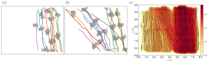
Figure 1: Overview of the experimental data. In (a) and (b) we show two examples of overhead frames recorded by the depth cameras. The depth field in (a) depicts a set of $N=N_{\rm A}=13$ pedestrians all taking the straight path (path A), while in (b) we provide an example of a more balanced pedestrian distribution. The gray shades represent the distance between each pixel and the camera plane (i.e. the elevation from the ground). This type of data allows reliable pedestrian tracking (see “Materials and Methods” for details). The automatic tracking output is overlayed as solid colored lines. (c) Heat-map of pedestrians position from the entire dataset. We remark that the colorbar is given in logarithmic scale. The streamlines of the (spatially binned) mean velocity vector are used in order to provide a visual representation of the most probable trajectories.

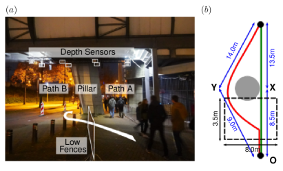
Figure 2: Experimental setup from the viewpoint of a pedestrian walking towards the path bifurcation (a) and sketch of the floor plan (b). A low fence blockage drives the pedestrian flow towards one same entrance point, while a set of bollards separates the bicycle lane from the adjacent road preventing pedestrians from entering the system from other locations or to exit by an area not covered by cameras. A grid of 4x2 Orbbec depth cameras, hanging below the overpass connecting the Philips stadium to a nearby train station, is used to collect trajectories within the area marked by dotted black lines in (b).

II Measurement campaign

We collected the trajectories used in the analysis presented in this paper during the GLOW light festival, in Eindhoven (The Netherlands), between November 9th and 16th 2019. The festival comprises a city-wide circular route, with mostly uni-directional traffic. We established our measurement setup along the outer perimeter of the Philips Stadium, few hundreds meters upstream and downstream from the festival’s light exhibitions. Pedestrians approaching the setup faced the non-symmetric binary choice of bypassing, on either side, a large support pillar (sustaining the stadium grandstands, Fig. 2(a)). On the right-hand side, the path, from now on referred to as path A, was approximately straight, with free sight of the horizon. The longer path on the left-hand side, path B, partially overlapping a bike lane (partially reserved to pedestrians), was rather curved around and following the pillar base (cf. Figures 2(a,b)). The crowd traffic in the area was stemmed by two types of barriers: several bollards placed on the side of path B separated the bicycle lane from the adjacent road, while a low fence directed the flow towards the path bifurcation from a single arrival basin.

The geometrical definition of the length of the two paths, respectively, $L_{\rm B}$ and $L_{\rm A}$, is subject to a certain degree of arbitrariness, depending on where the initial and final destination points are taken, and on the considered connected trajectories. We shall characterize the geometry of our setup via the non-dimensional constant

$$\lambda_{g}=\frac{L_{\rm B}}{L_{\rm A}}>1,$$ (1)

i.e. the ratio between the two paths lengths.

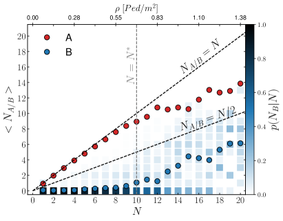
Figure 3: Average number of people taking path A ($\langle N_{\rm A}\rangle$, red dots) and B ($\langle N_{\rm B}\rangle$, blue dots) as a function of the global pedestrian count $N$. We observe that until $N<N^{*}=10$, on average less than one person opts to travel along path B. Above the $N^{*}$ threshold people start making systematic use of path B and both diagrams exhibit a clear change. The blue colorbars provide a visual representation of the probability distribution $P(N_{\rm B}|N)$ of number of people taking path B, conditioned to the global pedestrian count $N$. Even when $N>N^{*}$ configurations in which no pedestrian walks on path B are frequent.

In order to provide an estimate for $\lambda_{g}$, we consider two different approaches. In the first one, we consider the right-triangle OXY in Fig. 2(b), with vertexes defined by the path midpoint at the entrance of the setup, right at the end of the low fences blockage (“O”), and the midpoints of paths A (“X”) and B (“Y”) across the pillar. In this case it holds $\lambda_{g}\approx 1.06$. If we restrict ourselves to the area covered by the depth sensors, we can also define $\lambda_{g}$ as a ratio between the length of a typical trajectory in B and in A (cf. Fig. 1(c) which provides an overview of the trajectory data as a heat-map of pedestrian positions). Including the uncertainty in the definition of these typical trajectories, it holds $1.3\lesssim\lambda_{g}\lesssim 1.4$. We shall come back later to the analysis of $\lambda_{g}$ and on how it is perceived by single individuals.

In low density conditions, pedestrians opt for path A in the greatest majority of cases (e.g. for $N<10$ path A is preferred in $\approx 95\%$ of cases). This is shown in Fig. 3, where we report the local average occupancy of the two paths, respectively $\langle N_{\rm A}(N)\rangle$ and $\langle N_{\rm B}(N)\rangle$, calculated on uncorrelated frames as a function of the instantaneous count $N$ (see supplementary material). As the number of pedestrians increases, we observe that path B “activates” as people start to systematically opt for it. We denote with $N^{*}$ the global pedestrians count at which path B activates, which we define as the minimum value of $N$ at which, on average, at least one person takes path B; in our setup $N^{*}=10$.

The local occupancy of paths A and B exhibits clear slope changes around $N^{*}$. In flow terms, $N^{*}$ corresponds to the transition from a strongly unbalanced distribution, in which rarely a pedestrian is found walking along path B, towards a more balanced A–B load partition.

Figure 3 includes a visual representation of the conditioned probability of the occupancy of path B, given the global pedestrian count $N$, i.e. $P(N_{\rm B}|N)$. Even when $N$ is much larger than $N^{*}$, $P(N_{\rm B}|N)$ is bi-modal: path B remains often empty. For instance, at $N=20$ we observe that in about $10\%$ of the cases pedestrians choose to walk only along path A. This observation points to the presence of a collective dynamics in which pedestrians at times follow others rather than attempting to optimize the flow partitioning. So, how do pedestrian choose the path? A quantitative modeling of this peculiar aspect will be the focus of our analysis in the coming sections.

Different global and local pedestrian count levels (i.e. in either path A or B) reflect on different average walking velocities. Fig. 4(a) reports the (average) local walking velocity along paths A and B as a function of the local pedestrian count: $v_{J}=v_{J}(N_{J})$, with $J\in\{A,B\}$. In turn, Fig. 4(b) reports how velocity depends on the global pedestrian count. These correspondences between velocity and the density/pedestrians-count, generally dubbed fundamental diagrams, are the most commonly adopted tool for macroscopic descriptions of vehicular and pedestrian traffic (cf. e.g. Vanumu et al. (2017); Seyfried et al. (2005); Jelić et al. (2012); Bosina and Weidmann (2018)).

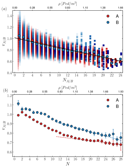
Figure 4: Fundamental velocity diagrams. (a) Local velocity as a function of the number of people present along path A (red) and path B (blue). Dots represent the average values, while colorbars synthesize the probability distribution functions. The black solid line provides a linear fit of the local velocity diagrams, under the reasonable assumption that the same fundamental diagram applies to both paths. (b) Global velocity as function of the total number of people in the system. We highlight an evident change in the slope of the diagram for both path A and path B for $N>N^{*}$, which we model (dotted lines) with a re-parametrization of the local velocity diagram. (see main text for details).

As the number of pedestrians increases, the average walking velocity decreases. Consistently with studies conducted in comparatively low-density regimes Seyfried et al. (2005), we observe, on average, a linear decay trend in the local fundamental diagrams:

$$\langle v_{J}(N_{J})\rangle=v_{0}-\kappa~{}N_{J},$$ (2)

where $v_{0}$ is the “free-stream velocity” in the zero-density limit and $\kappa$ fixes the diagram slope. We assume the local fundamental diagram to be the same, for people walking in path A and B. We have verified this by performing a fit for the parameters $v_{0}$ and $\kappa$, independently, for the two sets of pedestrians walking either of the two paths and observing no significant differences. In Fig. 4(a), we show with a solid line the best fit on the overall dataset, given by: $v_{0}\approx 1.012~{}\rm{m/s}$, $\kappa\approx 0.017~{}\rm{m/s\cdot 1/ped}$, with the coefficient of determination $R^{2}\approx 0.93$. Fig. 4(a) additionally reports the full conditioned probabilities $P(v_{J}|N_{J})$ that highlights velocity fluctuations, $\epsilon$, around the average. We shall address these as independent with respect to the pedestrian count $N$, and additive with respect to the average velocity, in particular

$$\epsilon\sim\mathcal{N}(\mu=0,\sigma=0.15),$$ (3)

where $\mathcal{N}$ is the Gaussian distribution, and the variance $\sigma$ has been estimated from the experimental data (see supplementary information). The global fundamental diagrams, $\langle v_{J}\rangle=\langle v_{J}(N)\rangle$ in Fig. 4(b), contrarily to their local counterparts, display qualitative and quantitative differences between the routes. For any value of $N$, the average walking velocity in path B is higher than in A:

$$\langle v_{\rm B}(N)\rangle>\langle v_{\rm A}(N)\rangle,\quad\forall N.$$ (4)

Second, we observe a change in slope, $\partial_{N}\langle v_{J}(N)\rangle$, around $N\approx N^{*}$ (we employ the symbol $\partial_{N}$ for the partial derivative $\partial/(\partial N)$). For $N<N^{*}$, the global diagram for path A coincides with its correspondent local diagram:

$$\langle v(N_{\rm A})\rangle\approx\langle v_{\rm A}(N_{\rm A})\rangle,\quad N<N^{*}.$$ (5)

This is natural since, in this range, $N_{\rm A}(N)\approx N$ holds (Fig. 3). On path B, the velocity as a function of $N$ decreases linearly, yet at a smaller rate than $-\kappa$ (i.e. $\partial_{N}\langle v_{\rm B}(N)\rangle<-\kappa$). When $N$ is small, path B is rarely employed (cf.  probability distribution function of the local density $N_{\rm B}$ in Fig. 3). This allows pedestrians to easily walk at their preferred walking speed (i.e. the free stream velocity $v_{0}$).

Conversely, when $N>N^{*}$, the activation of path B yields $N_{\rm A}(N)<N$. This reflects in the slower decay of $\langle v_{\rm A}(N)\rangle$ as $N$ increases in comparison with the local counterpart:

$$\partial_{N}\langle v_{\rm A}(N)\rangle<-\kappa,\quad N>N^{*}.$$ (6)

We can reconstruct the global fundamental diagram from the local diagram by considering $N_{J}=N_{J}(N)$. This yields

$$\partial_{N}\langle v_{J}(N)\rangle\approx-\kappa\partial_{N}N_{J}\big{|}_{N},\quad N>N^{*},$$ (7)

which satisfies (6) since $\partial_{N}N_{J}<1$ holds in the considered regime (cf. Fig. 3; see the dotted lines included in Fig. 4(b)).

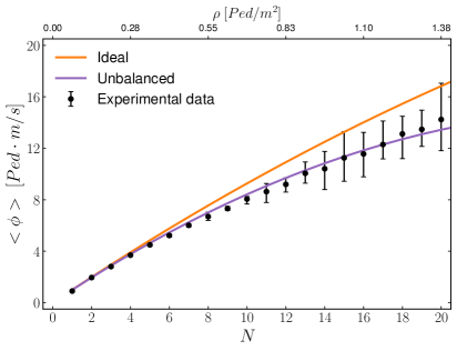
Figure 5: Average pedestrian flow (Eq. 8) as a function of the pedestrian count. The solid lines represent the theoretical maximum (orange color) and minimum (purple color) case scenarios. We observe that experimental results (black dots) on average closely follow the flow of the most unbalanced case. The error bars have been obtained by dividing the data into 10 bins, with the extrema of the error bars representing the minimum and maximum average value per bin.

We conclude this section turning our analysis to the pedestrians flow, which we define as:

$$\phi(N)=\langle v_{\rm A}(N_{\rm A})\rangle N_{\rm A}(N)+\langle v_{\rm B}(N_{\rm B})\rangle N_{\rm B}(N).$$ (8)

By making use of the fundamental velocity diagram, we can conveniently define a theoretical upper bound and lower bound for Eq. 8, which are found respectively in correspondence of the optimal partitioning $N_{\rm A}(N)=N/2$, and the most unbalanced case $N_{\rm A}(N)=N$ (or likewise $N_{\rm A}(N)=0$). The above holds under the assumption that the section of path A equals that of path B, which is approximately true in our setup. Combining this information with the velocity fundamental diagram in Eq. 2, we can define

$$\phi_{\rm ideal}(N)=v_{\rm A}\left(\frac{N}{2}\right)N,\quad\phi_{\rm unbalanced}(N)=v_{\rm A}(N)N.$$ (9)

In Fig. 5 we compare the experimental data with the modeling from Eq. 9. The slope $\kappa$ determines the differences between the upper bound and lower bound, which in the density range considered are at most $20\%$. Nevertheless a clear trend emerges, with the experimental data closely following (on average) the flow of the highly unbalanced configuration; this provides clear-cut evidence for pedestrians not managing to maximize the global throughput, despite the simplicity of the setup.

On these bases, in the following section we introduce a model for studying the routing behavior and the features arising at the transition around $N\approx N^{*}$, and where we assume that pedestrians aim at optimizing their benefit (perceived travel time to destination).

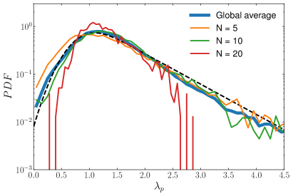
Figure 6: Probability distribution function (PDF) of the perceived path length ratio $\lambda_{p}$ (cf. (18)). We report the distribution for for three different global density values, respectively at low ($N=5$), intermediate ($N=10$) and high ($N=20$) density values. The blue line shows the PDF obtained considering the overall dataset, with the black dotted line representing a fit making use of an exponentially modified Gaussian (see Eq. 20), with mean $\mu=0.77$ and standard deviation $\sigma=0.30$, and an exponential distribution with scale parameter $\beta=0.68$.

III Results

III.1 Model

We aim at a minimal model exposing the underlying mechanisms involved in the routing decision.

Although a time-dependent model for the probability of choosing either paths, already pursued by the same authors Gabbana et al. (2021), appears like a natural choice, its success is enslaved to the comprehension of the complex time correlation characterizing the choice process, or to phenomenological data-fitting Gabbana et al. (2021); Wagoum et al. (2017).

The short duration of the festival, the relatively limited number of tracking hours, and the high variability in the crowd, make a time correlation analysis extremely challenging. Therefore, aiming at a bottom-up physical model, we pursue a time-independent approach.

We consider a simulated crowd of $N$ pedestrians indexed by $i=1,\ldots,N$ about to cross the experiment area in Fig. 2. We allow each individual to choose between path A or B in awareness of the choice of others. This gives configurations $c$ in the form of

$$c=(J^{(1)},J^{(2)},\ldots,J^{(N)}),$$ (10)

where $J^{(i)}$ equals $A$ or $B$ depending on the path selected by the the $i$-th pedestrian.

Let $v^{(i)}_{J}=v^{(i)}_{J}(N_{J})$ be the walking velocity of the $i$-th pedestrian on path $J$ as a function of the local density $N_{J}$, i.e. the local fundamental diagram (cf. (2), (3)). We define the perceived travel time

$$\tau^{(i)}_{J}=g^{(i)}_{J}\left(\frac{L_{J}}{v^{(i)}_{J}(N_{J})}\right)$$ (11)

in either paths to be a key variable in the A vs. B choice; here $g^{(i)}_{J}(\cdot)$ is a function mapping the actual “geometric” travel time $L_{J}/v^{(i)}_{J}$ to the perceived one. The expression of $g^{(i)}_{J}$ will be discussed later on.

We consider a variational framework in which path choices are such that the minimum for the crowd-level functional

$$\mathcal{L}=\mathcal{L}(\tau^{(1)}_{J_{1}},\ldots,\tau^{(N)}_{J_{N}}),$$ (12)

is attained. We consider a dynamics in which pedestrians arrange to reduce the total perceived travel time:

$$\mathcal{L}=\sum_{i=1}^{N}\tau^{(i)}_{J_{i}}.$$ (13)

Defining the discomfort functional $\mathcal{L}$ is the modeling endeavor: the choice is not unique, yet (13) gave us the best agreement with observations; the interested reader will find a comparison with a model adopting a different choice for $\mathcal{L}$ in the supplementary information.

To summarize, we consider a system that takes the configuration $c^{*}\in\Gamma$ for which

$$\min_{c\in\Gamma}\left[\sum_{i=1}^{N}\tau^{(i)}_{J_{i}}\right]=\min_{c\in\Gamma}\left[\sum_{i=1}^{N}g^{(i)}_{J}\left(\frac{L_{J}}{v^{(i)}_{J}(N_{J})}\right)\right],$$ (14)

with $\Gamma$ representing the full set of $2^{N}$ distinct configurations, and with the individual velocities (cf. (2)) satisfying

$$v^{(i)}(N_{J})=v_{0}-\kappa~{}N_{J}+\epsilon^{(i)},$$ (15)

with $\epsilon^{(i)}$ independent and identically distributed realization of (3).

Notably, the case $\epsilon^{(i)}=0$, $g^{(i)}_{J}(x)=x$ (i.e. deterministic velocity, and no fluctuations in the perception of the path-length) reduces to a Hughes-like model Hughes (2003), and has the analytic solution in terms of optical lenghts:

$$\frac{L_{\rm A}}{v_{\rm A}(N_{\rm A})}=\frac{1}{\sqrt{\lambda_{g}}}\frac{L_{\rm B}}{v_{\rm B}(N_{\rm B})}\quad,$$ (16)

where we have dropped the index $i$ since pedestrians are now indistinguishable from each others. The above implies the following expression for $N_{\rm A}=N_{\rm A}(N)$:

$$N_{\rm A}(N)=\min\left\{N,\frac{\kappa N+v_{0}(\sqrt{\lambda_{g}}-1)}{\kappa(\sqrt{\lambda_{g}}+1)}\right\}\quad.$$ (17)

Moreover, from Eq. S3 we can define a link between $\lambda_{g}$ and the local velocity of pedestrians in path A and B: $\lambda_{g}=\left(\frac{v_{\rm B}(N_{\rm B})}{v_{\rm A}(N_{\rm A})}\right)^{2}$. The above expression suggests an alternative pathway for measuring $\lambda_{g}$ directly from experimental data. To this aim, we introduce the instantaneous quantity

$$\lambda_{p}(t)=\left(\frac{\hat{v}_{\rm B}(t)}{\hat{v}_{\rm A}(t)}\right)^{2},$$ (18)

where $\hat{v}_{\rm B}$ (resp. $\hat{v}_{\rm A}(t)$) indicates the average walking speed of pedestrians in path B (resp. A) measured at time $t$.

In Fig. 6, we show the probability distribution function (PDF) of $\lambda_{p}$, for the overall dataset, and also conditioned on a few selected values of $N$; we report three representative examples at low, intermediate and large density values (PDFs are restricted to meaningful cases $N_{\rm A},N_{\rm B}>0$). Two aspects emerge. The modal value, $\mbox{mode}(\lambda_{p})\approx 1.2$, of the distributions is independent on the global pedestrian count $N$, consistently with the deterministic model in (S3). While, $\mbox{mode}(\lambda_{p})$ is comparable with the estimates of $\lambda_{g}$ provided in the previous section, we observe that the distributions for $\lambda_{p}$ are skewed and carry heavy tails, in particular at low densities.

These are due to observed configurations strongly departing from the deterministic optimum in (S3). Right tails corresponds to cases in which many pedestrians walk along path A even though it might have been less costly (in $\mathcal{L}$ terms) to take B. This can be motivated considering that opting for path B involves traveling around an obstacle which hides the horizon and to invade the (temporarily closed) bike lane.

The variance of the distributions decreases with the global density. This is consistent with the fact that for $N>N^{*}$ the load between A and B gets (on average) increasingly balanced, conversely, the herding becomes weaker (see Fig. 3).

In the next section, we compare Monte Carlo simulations of the dynamics considering various models for $\lambda_{p}$, which we integrate in (13)-(14) by defining the conversion functions $g^{(i)}_{J}(\cdot)$ as $i$-independent (i.e. pedestrian-independent) rescaling factors

$$g_{A}\left(\frac{L_{\rm A}}{v_{A,i}(N_{\rm A})}\right)=\frac{L_{\rm A}}{v_{A,i}(N_{\rm A})}$$

$$g_{B}\left(\frac{L_{\rm B}}{v_{B,i}(N_{\rm B})}\right)=\frac{\lambda_{p}}{\lambda_{g}}\frac{L_{\rm B}}{v_{B,i}(N_{\rm B})}=\lambda_{p}\frac{L_{\rm A}}{v_{B,i}(N_{\rm B})}.$$ (19)

Following the PDF in Fig. 6, we fit $\lambda_{p}$ with an $N$-independent exponentially modified Gaussian distribution (i.e. the sum of independent normal and exponential random variables):

$$\lambda_{p}=X+Y,$$ (20)

where $X\sim\mathcal{N}(\mu=0.77,\sigma=0.30)$ and $Y\sim\mbox{Exp}(\beta=0.68)$, where $\beta$ is the scale parameter of the exponential distribution; observe that the expected value is given by $E[X+Y]=\mu+\beta=1.45$.

III.2 Numerical Results

While the deterministic version of the model offers access to a simple analytic solution (S3), this is not the case for the non-deterministic model (Eqs. (14-15-19-20)). Therefore, to perform our analysis and compare with measurements we rely on Monte Carlo simulations to identify the statistics of optimal configurations in dependence on the stochastic terms considered: $c^{*}=c^{*}(\lambda_{p},\epsilon^{(1)},\ldots,\epsilon^{(N)})$.

In Fig. 7(a) we compare the model and experimental data on the average number of people taking path A, $<N_{\rm A}>$, conditioned to the global density $N$. The numerical results provide a good description of the measurements, and, in particular, they capture the transition at $N^{*}$.

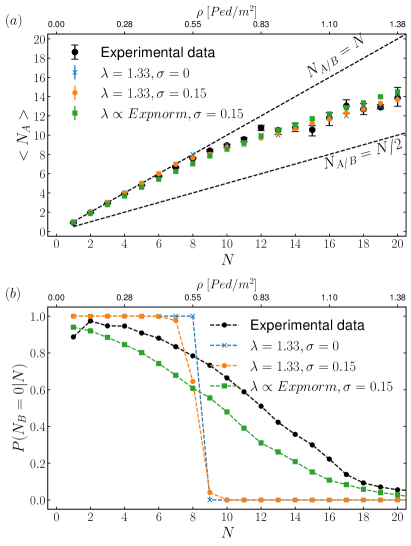
Figure 7: Comparison of numerical results from simulations against experimental data. (a) $<N_{\rm A}(N)>$: the average number of people taking path A as a function of the global pedestrian count $N$. (b) $P(N_{\rm B}=0|N)$, the Bernoulli probability of observing configurations in which no pedestrians walk across path B, conditioned on the global pedestrian count $N$. It is evident that fluctuations on the perceived path length allow a more realistic description of the transition around $N^{*}$, as shown in b), still correctly capturing the average behavior, as shown in a).

The model is capable of reproducing, with very good accuracy, also the footprints of the herding effect: this is shown Fig. 7(b), reporting the (Bernoulli) probability of observing exactly zero pedestrians walking along path B, conditioned to $N$ (i.e. $P(N_{\rm B}=0|N)$). In order to obtain a good agreement between experimental data and simulations we have tuned the parameters of the distribution from which $\lambda_{p}$ is drawn; the results presented in this section make use of Eq. 20 with $X\sim\mathcal{N}(\mu=1.15,\sigma=0.20)$ and $Y\sim\mbox{Exp}(\beta=0.33)$.

With the aim of exposing the role of random fluctuations, in Fig. 7 we show the results obtained by employing a fully deterministic model (i.e. with a deterministic fundamental velocity diagram, $\epsilon^{(i)}=0$, and with a constant value for $\lambda_{p}$) as well as a case in which we allow fluctuations in the velocity, but no stochasticity on $\lambda_{p}$.

The deterministic model well captures the average routing choice performed by pedestrians, as shown in Fig. 7(a). On the other hand, it also highlights a sharp transition at $N^{*}$ (see Fig. 7(b)): when $N<N^{*}$ all pedestrians systematically route for path $\rm A$, while for $N>N^{*}$ the optimal configurations do not allow for cases in which exactly zero pedestrians are found walking along path B.

When including fluctuations in the velocity (orange curves) we obtain two relevant effects connected to each other. The walking speed variability creates (rare) optimal configurations $c^{*}$ with pedestrians on path B, even at density values $N<N^{*}$; this effect, only slightly visible in Fig. 7(b), becomes more pronounced as the variance associated to $v_{0}$ is increased, in turn leading to a smaller predicted value for $N^{*}$ .

Introducing fluctuations in the model is crucial to provide an accurate description of the variability observed in the experimental data. This is clearly shown in Fig. 8, where we plot the probability distribution function for the number of people walking along path B, conditioned to the global count $N$. The figure reports three representative examples corresponding to different values of $N$. For low density values, the PDFs show a strong peak at $N_{\rm B}=0$. As $N$ increases, the bins corresponding to $N_{\rm B}>0$ start populating and, eventually, a bi-modal distribution emerges, together with an increased variability in the observed configurations.

Comparing once again the numerical results with the experimental data we can observe that the deterministic model cannot be used to describe the variability observed in the data, although it can provide an approximation to the average of PDFs. While introducing fluctuations in the pedestrians velocity only slightly increases the variability of the PDFs for $N>N^{*}$, it is only with the superposition of the herding effect (green curves) that the model is able to provide a good description of the PDFs. Remarkably, we are able to reproduce to good accuracy also the spikes in correspondence of $N_{\rm B}=0$ at large values of $N$.

In conclusion, we have shown that fluctuations are crucial for giving a realistic representation of the behaviors observed around $N\approx N^{*}$.

IV Discussion

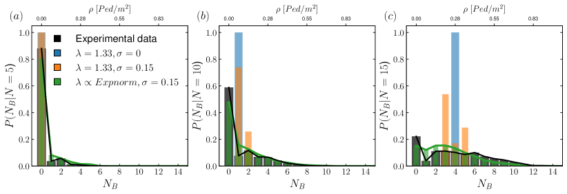
Figure 8: Probability distribution function of number of people in path B, $N_{\rm B}$, conditioned on the global count $N$. We report three examples, representative of three different levels of density: from left to right $N=5,10,15$. The experimental data (black bars) are compared against the results obtained employing three different models: In blue the results obtained employing a deterministic model in which individual fluctuations are neglected, in orange the results of a stochastic model accounting for fluctuations in individuals free-stream velocities, and finally in green the results of a stochastic model accounting for fluctuations in both free-stream velocities and path length perception for single individuals.

In this work, we have exposed the crucial role played by individual variability in pedestrians routing choices. Fluctuations emerge as a key element in explaining (intermittent) transitions from highly unbalanced to more balanced configurations which, on average, lead to a sub-optimal traffic partitioning.

We have based our analysis on a large dataset of pedestrian trajectories collected during an unprecedented high-accuracy pedestrian tracking campaign. We have considered a simplified setup in which a unidirectional pedestrian flow is confronted with a binary choice between two paths, presenting marginal differences in terms of length and geometrical complexity. We regard this setup as an excellent prototype for more complex scenarios where, e.g., the trajectory of a pedestrian results from the concatenation of multiple binary choices.

We have developed a time-independent variational model, which has allowed to successfully describe, both at a qualitative and quantitative level, the observed macroscopic patterns. Our modeling shows that we can explain the crowd behavior by considering a crowd-level minimization of the estimated traveling time, and accounting for the inherent stochasticity of (i) the walking speed of each single pedestrian, and (ii) the estimation of the path length.

In spite of the simplicity of the experimental setup, our analysis highlights a systematic deviation from global optimum configurations, leading to the global pedestrian throughput not being maximized. Additionally, further and sudden capacity drops appear due to the occurrence of herding behaviors - in which the crowd blindly opt for a highly sub-optimal “follow the lead” choice, rather than completely leveraging the allowed walking space. We remark that in our analysis we use the word herding in a broad sense, including both following effects as well as the presence of social groups attending the event. This choice is due to the fact that groups cannot be easily identified in the relatively short-scales of the experiment presented in this work, something on the other hand possible when observing trajectories in a much larger space/time frame Pouw et al. (2020).

These results clearly point towards the necessity of implementing efficient crowd management measures in order to increase comfort and safety, based on a deeper understanding of the physics of crowds.

To conclude, in this work we have introduced an approach for analyzing the statistics and the efficiency of macroscopic crowd configurations, highlighting an intrinsic sub-optimality in the natural flow of pedestrians, while setting a standard for effective quantitative modeling.

Data availability

The dataset with the pedestrian trajectories used in our analysis is available at https://doi.org/10.5281/zenodo.7007358, whereas examples and processing scripts can be found at https://github.com/crowdflowTUe/2022_fluctuations_in_routing_glow.

Supplementary Information for
“Fluctuations in pedestrian dynamics routing choices”

Experimental Setup

The trajectories used in the analysis presented in this work have been collected during the 2019 edition of the GLOW light festival in Eindhoven (The Netherlands). The experiment lasted the entire duration of Glow 2019, from November 9th until November 16th, 2019. The tracking was performed during the festival opening hours, every day from 18:00 until 00:00. The data collected on the 14th of November has not been included in the analysis, since on that day the experimental setup was modified in order to evaluate the impact of changing the lighting conditions on the crowd dynamic.

In Fig. S1 we show the pedestrian count as a function of time, with a inset highlighting the fluctuations in the number of pedestrians observed in a 15 minute window.

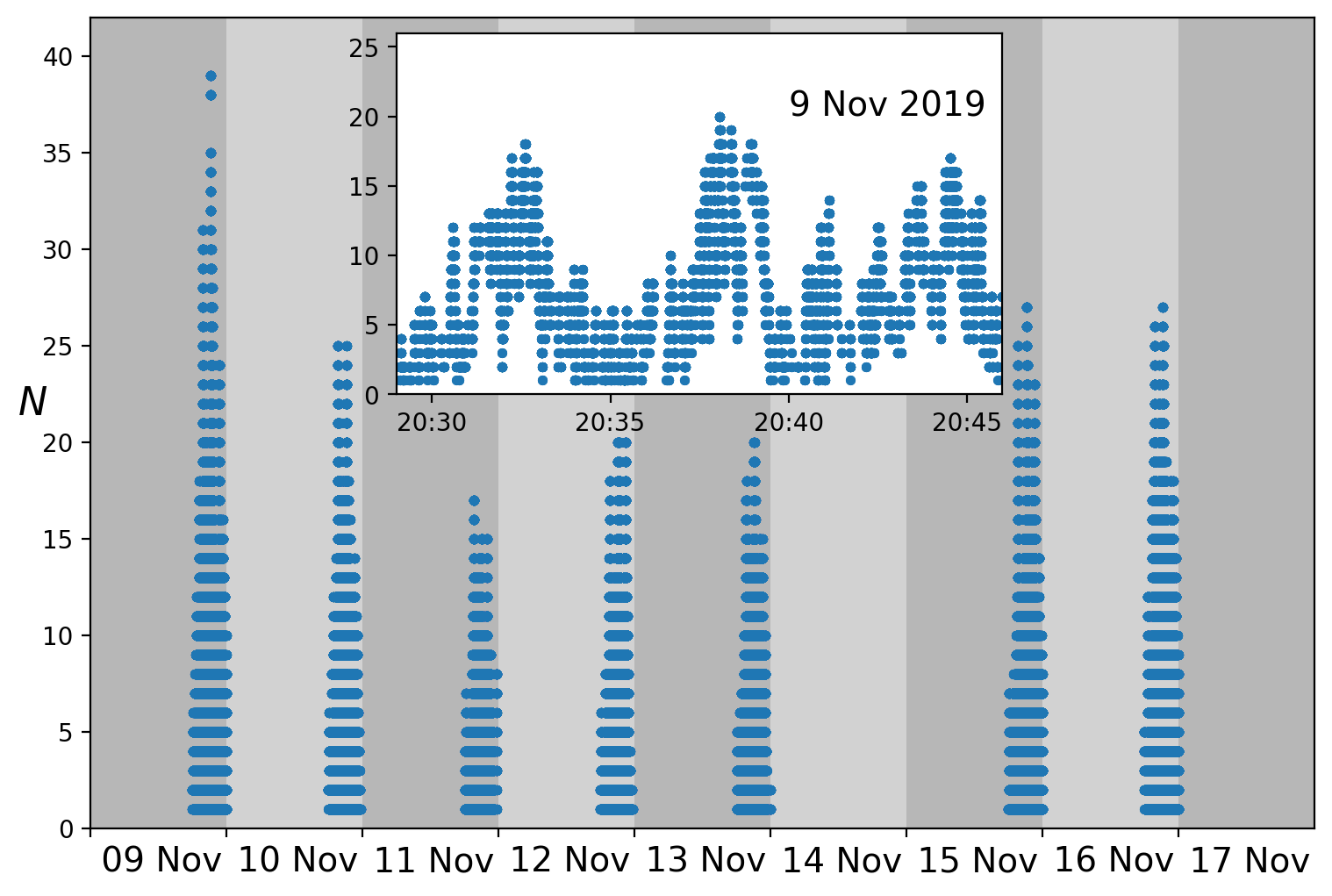
Figure S1: Pedestrian global count, $N$, as a function of time during the 8 days of the festival. The inset shows the fluctuations in the number of pedestrians observed in a 15 minute window around 20.40 during the first day of the experiment, highlighting the presence of both low and high density scenarios. The data collected on the 14th of November has not been used in our analysis since the experimental setup had been employed in a modified form and with a different purpose.

Pedestrian Sensing

We collected raw depth images of a walkable area of about $30\,m^{2}$ via 8 Orbbec Persee sensors attached underneath a pedestrian overpass, and arranged in a 4x2 grid (see Fig. 2 in the main text). The depth cameras acquired images at a frame rate of $30\,$Hz. The trajectories have been obtained from the raw depth images via the Height-Augmented Histogram of Oriented Gradients algorithm (HA-HOG) (see Kroneman et al. (2020) and  Corbetta et al. (2018, 2020) for detailed explanations on pedestrian tracking via depth sensor grids).

In Fig. S2 we show a depth map example with the trajectories resulting from the tracking of the 10 pedestrians in overlay.

The black dotted lines represent the raw trajectories, obtained by applying the HA-HOG algorithm. Solid lines represent the result of applying a Savitzky-Golay filter Savitzky and Golay (1964) to the trajectories. This operation allows to reduce the level of noise and discontinuities which affect the calculation of derivatives, used, for example, to estimate the instantaneous velocity of pedestrians:

$$\bm{v}(t)=\left(\frac{\tilde{s}_{x}(t+\Delta t)-\tilde{s}_{x}(t)}{\Delta t},\frac{\tilde{s}_{y}(t+\Delta t)-\tilde{s}_{y}(t)}{\Delta t}\right)$$ (S1)

where $\tilde{\bm{s}}(t)$ represents the spatial position within the trajectory of a pedestrian at time $t$ after having applied the Savitzky-Golay filter, and $\Delta t=1/30\rm{s}$ follows from the cameras aquisition rate.

Data analysis

Refinement of the dataset

In the analysis we have considered only configurations from uni-directional flows. We have dropped all trajectories of pedestrians traveling in the opposite direction with respect to the viewpoint in Fig. 2 in the main text, as well as all trajectories interacting directly or indirectly with them, i.e. both being present at the same time in at least one frame, or sharing a frame with a pedestrian who has previously interacted with a trajectory going in the opposite direction.

Although the bike lane adjacent to the experimental setup was supposedly closed to traffic during the festival hours, cyclists and runners were still present and able to access it from the street. In order to drop from the dataset cyclists, runners, as well as people standing still under the area covered by our sensors, we have retained trajectories with instantaneous velocities $v(t)$ in the interval of $[0.05,2.9]~{}\rm{m/s}$ and average velocity $\langle v\rangle$ of $[0.15,1.5]~{}\rm{m/s}$.

Throughout the week, we have collected $192,229$ individual trajectories. Following the above discussion, the analysis retains $101,867$ among these trajectories.

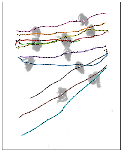
Figure S2: Snapshot of data recorder by the depth cameras. The black dotted lines represent the trajectories of each pedestrian, obtained by applying the HA-HOG algorithm. Solid lines have been obtained by applying a Savitzky-Golay filter.

Data de-correlation

The calculation of the average number of pedestrians walking in each path as a function of the global pedestrian count requires extra care due to presence of strong correlations between consecutive frames.

For this reason, in our analysis we have taken into consideration only configurations at least $4$ seconds apart from each other. This value is larger than the average time duration of a single trajectory, which in our data corresponds to $\approx 3.9$ seconds.

In Fig. S3 we show the number of frames contributing to the statistics of pedestrians walking in path A and B as a function of the global pedestrian count. Dots represent the full dataset, whereas triangles represent the uncorrelated dataset.

For the calculation of the local and global velocity fundamental diagram we have made use of the full dataset, since, in this case, time correlations do not introduce biases in the analysis.

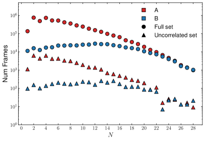
Figure S3: Number of frames contributing to the statistics of pedestrians walking in path A and B as a function of the global pedestrian count. Dots represent the full dataset, which we use to compute statistics on (and related to) the velocity of pedestrians. Triangles represent the dataset consisting of uncorrelated configurations, taken at least $4$ seconds apart from each other, which we use to compute statistics on (and related to) the pedestrian count. The plot gives an indication of the statistical resolution of our analysis.

Estimation of fluctuations in the velocity fundamental diagram

In Eq.3 in the main text we define an additive noise term $\epsilon$ for the fundamental velocity diagram, with $\epsilon$ drawn from a Gaussian distribution with zero mean and variance $\sigma=0.15$. We have estimated $\sigma$ from the the average fluctuations of the local pedestrian velocity in dependence of $N_{\rm A}$ and $N_{\rm B}$, as reported in Fig. S4.

In Fig. S4, we show the average fluctuations of the local pedestrian velocity in dependence of $N_{\rm A}$ and $N_{\rm B}$. The plot shows the average standard deviation from the (local) average velocity, computed on frames featuring the same number of pedestrians respectively in path A and path B. We observe that, within error bars, $\sigma$ is constant and independent of $N_{\rm A}$ and $N_{\rm B}$.

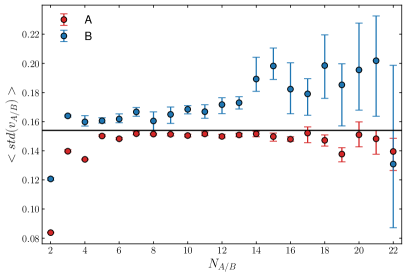
Figure S4: Average fluctuations of the local pedestrian velocity in dependence of $N_{\rm A}$ and $N_{\rm B}$, calculated from the experimental data. The plot shows the average standard deviation from the (local) average velocity, computed on frames featuring the same number of pedestrians respectively in path A and path B. The black line represents the global average value of $\sigma=0.154$.

Comparison with a different routing policy

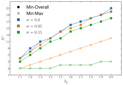
Figure S5: Comparison of two routing policies, the min-overall policy presented in the main text, and the min-max policy included in the supplementary material. The plot shows the threshold value $N^{*}$ calculated from simulations using different values of $\lambda_{g}$. We highlighting the effect of introducing fluctuations ($\sigma$) on pedestrians walking speed. While the two policies provide very similar results in the deterministic case ($\sigma=0$), we observe that strong differences arise when including fluctuations. In particular, for values of $\sigma$ comparable with those observed in the experimental data ($\sigma=0.15$), the min-max policy favors the use of path B at a much earlier stage with respect to what observed in the experiment. (cf. Fig. 7 in the main text).

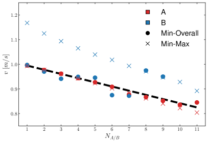
Figure S6: Local velocity diagram calculated from two simulations with $\sigma=0.1$, $\lambda_{g}=1.7$ for the min-max policy, and $\lambda_{g}=1.3$ for the min-overall policy. The black dotted line shows the linear fit of the experimental data, which is used in simulations to determine the velocity of pedestrians. The plot shows that the min-max policy introduces a systematic selection mechanism, which leads to placing fast walkers in path B, a feature which does not emerge from the experimental data.

In the main text we have presented numerical results making use of a variational principle implementing a policy in which pedestrians arrange themselves in order to minimize the overall traversal time. This policy is de facto equivalent to imposing the minimization of the average traversal time.

We here consider an alternative policy, in which pedestrians perform routing choices by minimizing the worst case scenario, i.e. the traveling time of the person that takes the longest to reach destination. The discomfort functional in this case reads as

$$\mathcal{L}=\max_{i}\tau^{(i)}_{J_{i}}.$$ (S2)

Even in this case, when neglecting stochastic terms the model reduces to a Hughes-like form Hughes (2003), with the analytic solution $N_{\rm A}=N_{\rm A}(N)$ defined by the relation

$$\frac{L_{\rm A}}{v_{\rm A}(N_{\rm A})}=\frac{L_{\rm B}}{v_{\rm B}(N_{\rm B})}=\lambda_{g}\frac{L_{\rm A}}{v_{\rm B}(N_{\rm B})}\quad,$$ (S3)

from which it directly follows

$$\lambda_{g}=\frac{v_{\rm B}(N_{\rm B})}{v_{\rm A}(N_{\rm A})}\quad.$$ (S4)

We remark that $\lambda_{g}$ is equal to the velocity ratio between path B and A, at variance with the minimum-overall policy reported in the main text where $\lambda_{g}$ was instead put in relation with the square of the velocity ratio. We take this aspect into account in the comparison of the two different policies. In Fig. S5 we plot the results of the policy minimizing the worst case scenario (Eq. S2, “min-max” henceforth) in correspondence of the square of value of $\lambda_{g}$ used in simulations, in order to make it directly comparable with the min-overall policy.

In Fig. S5 we compute the threshold value $N^{*}$ for different values of $\lambda_{g}$, comparing the two different policies. When considering the deterministic case (respectively Eq. S3 and Eq.16 in the main text) we observe that the two policies provide very similar results. However, strong differences arise when including fluctuations in the local velocity diagram. When pedestrians with different walking speed are present, the min-max policy favors the use of path B at a much earlier stage with respect to the min-overall policy; crucially, the latter provides a more accurate description of the experimental data, since with $\lambda_{g}=1.33$ and $\sigma=0.15$ we correctly reproduce the transition at $N^{*}$ (see again Fig. 7 in the main text). Reproducing these results with the min-max policy, by accounting for the fluctuations observed in the velocity diagram, would require an (artificially) larger value of $\lambda_{g}$.

In Fig. S6 we present a second evidence in support to the fact that the min-overall policy provides a more accurate description of the experimental data. In the figure we show a sort of self-consistency check, by calculating the local velocity diagram from two simulations with $\sigma=0.1$, $\lambda_{g}=1.7$ for the min-max policy, and $\lambda_{g}=1.3$ for the min-overall policy. The black dotted line represents the linear fit of the experimental data, used in simulations to determine the velocity of pedestrians. The plot shows that the min-max policy introduces a systematic selection mechanism, which leads to placing fast walkers in path B, a feature which does not emerge from the experimental data (cf. Fig. 4a in the main text).

Relationship between pedestrian count and density

In this work we have considered a time-independent modeling approach, which has allowed us to neglect complex time correlations whose comprehension would have required much more statistics. Within this framework we have found convenient to take into consideration for our analysis the pedestrian count $N$. As already stated in the main text, this quantity can be put in relationship with the density $\rho$ via

$$\rho=\frac{N}{A},$$ (S5)

with $A$ the measurement area.

The overall area covered by our depth cameras (Fig. 2) consists of approximately $A\approx 28~{}\rm{m^{2}}$. However, using such value for $A$ would lead to an underestimation of the density since the measured trajectories do not uniformly distribute on the measurement area because of the geometry and typical flow conditions.

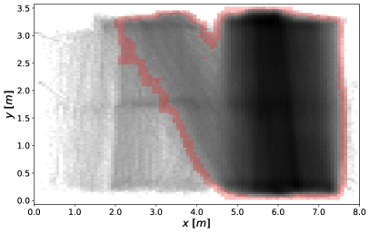
Figure S7: Boundary (red line) of the reference area ($A_{\rm ref}$) used in the estimation of the pedestrian density ($\rho$). The probability distribution function of the pedestrian positions, used in the definition of $A_{\rm ref}$, is shown in logarithmic scale (grayscale colormap).

Therefore, we compute the density with respect to an effective area $A_{\rm ref}$, shaped after the effective floor usage.

In order to calculate $A_{\rm ref}$ we have applied a threshold to the probability distribution function of the pedestrian positions (2d-histogram in Fig. 1c). This corresponds to the region bounded by the red line in Fig. S7, which represents a domain contributing the $99\%$ of the occupancy probability. This yields $A_{\rm ref}=14.67~{}\rm{m^{2}}$.

References

- Hughes (2003) R. L. Hughes, Annual Review of Fluid Mechanics 35, 169 (2003).
- Seneviratne and Morrall (1985) P. N. Seneviratne and J. F. Morrall, Transportation Planning and Technology 10, 147 (1985).
- Hoogendoorn and Bovy (2004a) S. P. Hoogendoorn and P. H. L. Bovy, Transportation Research Part B 38, 169 (2004a).
- Hoogendoorn and Bovy (2004b) S. P. Hoogendoorn and P. H. Bovy, Transportation Research Part B: Methodological 38, 571 (2004b).
- Brown et al. (2007) B. B. Brown, C. M. Werner, J. W. Amburgey, and C. Szalay, Environment and behavior 39, 34 (2007).
- Mehta (2008) V. Mehta, Journal of Urbanism 1, 217 (2008).
- Guo and Loo (2013) Z. Guo and B. P. Loo, Journal of transport geography 28, 124 (2013).
- Shatu et al. (2019) F. Shatu, T. Yigitcanlar, and J. Bunker, Journal of Transport Geography 74, 37 (2019).
- Sevtsuk and Kalvo (2020) A. Sevtsuk and R. Kalvo, International Journal of Sustainable Transportation , 1 (2020).
- Campanella et al. (2009) M. Campanella, S. P. Hoogendoorn, and W. Daamen, Transportation research record 2124, 148 (2009).
- Hughes (2002) R. L. Hughes, Transportation Research Part B: Methodological 36, 507 (2002).
- Marchetti et al. (2013) M. C. Marchetti, J. F. Joanny, S. Ramaswamy, T. B. Liverpool, J. Prost, M. Rao, and R. A. Simha, Rev. Mod. Phys. 85, 1143 (2013).
- Oettler et al. (2013) J. Oettler, V. S. Schmid, N. Zankl, O. Rey, A. Dress, and J. Heinze, PLOS ONE 8, 1 (2013).
- Leyden (2003) K. M. Leyden, American journal of public health 93, 1546 (2003).
- Blanco et al. (2009) H. Blanco, M. Alberti, A. Forsyth, K. J. Krizek, D. A. Rodriguez, E. Talen, and C. Ellis, Progress in Planning 71, 153 (2009).
- Cristiani and Peri (2019) E. Cristiani and D. Peri, Applied Mathematical Modelling 72, 553 (2019).
- Helbing and Molnár (1995) D. Helbing and P. Molnár, Phys. Rev. E 51, 4282 (1995).
- Helbing et al. (2000) D. Helbing, I. Farkas, and T. Vicsek, Nature 407, 487 (2000).
- Blue and Adler (1998) V. J. Blue and J. L. Adler, Transportation Research Record 1644, 29 (1998).
- Blue and Adler (2001) V. J. Blue and J. L. Adler, Transportation Research Part B: Methodological 35, 293 (2001).
- Hughes (2000) R. Hughes, Mathematics and Computers in Simulation 53, 367 (2000).
- Treuille et al. (2006) A. Treuille, S. Cooper, and Z. Popović, ACM Transactions on Graphics (TOG) 25, 1160 (2006).
- Duives et al. (2013) D. C. Duives, W. Daamen, and S. P. Hoogendoorn, Transportation research part C: emerging technologies 37, 193 (2013).
- Borgers and Timmermans (1986) A. Borgers and H. Timmermans, Geographical analysis 18, 115 (1986).
- Verlander and Heydecker (1997) N. Q. Verlander and B. G. Heydecker, Transportation planning methods Volume 11. Proceedings of seminar F held at PTRC European Transport Forum P415, 1 (1997).
- Koh and Wong (2013) P. Koh and Y. Wong, Journal of Environmental Psychology 36, 202 (2013).
- Kretz et al. (2006a) T. Kretz, A. Grünebohm, M. Kaufman, F. Mazur, and M. Schreckenberg, Journal of Statistical Mechanics: Theory and Experiment 2006, P10001 (2006a).
- Kretz et al. (2006b) T. Kretz, A. Grünebohm, and M. Schreckenberg, Journal of Statistical Mechanics: Theory and Experiment 2006, P10014 (2006b).
- Seyfried et al. (2010) A. Seyfried, M. Boltes, J. Kähler, W. Klingsch, A. Portz, T. Rupprecht, A. Schadschneider, B. Steffen, and A. Winkens, Pedestrian and Evacuation Dynamics 2008 , 145 (2010).
- Moussaïd et al. (2011) M. Moussaïd, D. Helbing, and G. Theraulaz, Proceedings of the National Academy of Sciences 108, 6884 (2011).
- Zhang et al. (2012) J. Zhang, W. Klingsch, A. Schadschneider, and A. Seyfried, Journal of Statistical Mechanics: Theory and Experiment 2012, P02002 (2012).
- Tong and Bode (2022) Y. Tong and N. W. Bode, Journal of the Royal Society Interface 19, 20220061 (2022).
- Moussaïd et al. (2012) M. Moussaïd, E. G. Guillot, M. Moreau, J. Fehrenbach, O. Chabiron, S. Lemercier, J. Pettré, C. Appert-Rolland, P. Degond, and G. Theraulaz, PLOS Computational Biology 8, 1 (2012).
- Bongiorno et al. (2021) C. Bongiorno, Y. Zhou, M. Kryven, D. Theurel, A. Rizzo, P. Santi, J. Tenenbaum, and C. Ratti, Nature Computational Science 1, 678 (2021).
- Brščić et al. (2013) D. Brščić, T. Kanda, T. Ikeda, and T. Miyashita, IEEE Trans. Human-Mach. Syst. 43, 522 (2013).
- Seer et al. (2014) S. Seer, N. Brändle, and C. Ratti, Transport. Res. C-Emer. 48, 212 (2014).
- Corbetta et al. (2014) A. Corbetta, L. Bruno, A. Muntean, and F. Toschi, Transportation Research Procedia 2, 96 (2014).
- Willems et al. (2020) J. Willems, A. Corbetta, V. Menkovski, and F. Toschi, Scientific reports 10, 1 (2020).
- Kroneman et al. (2020) W. Kroneman, A. Corbetta, and F. Toschi, Collective Dynamics 5, 33 (2020).
- Corbetta et al. (2017) A. Corbetta, C.-m. Lee, R. Benzi, A. Muntean, and F. Toschi, Phys. Rev. E 95, 032316 (2017).
- Corbetta et al. (2018) A. Corbetta, J. A. Meeusen, C.-m. Lee, R. Benzi, and F. Toschi, Phys. Rev. E 98, 062310 (2018).
- Brščić et al. (2014) D. Brščić, F. Zanlungo, and T. Kanda, Transportation Research Procedia 2, 77 (2014).
- Vanumu et al. (2017) L. D. Vanumu, K. R. Rao, and G. Tiwari, European transport research review 9, 1 (2017).
- Seyfried et al. (2005) A. Seyfried, B. Steffen, W. Klingsch, and M. Boltes, Journal of Statistical Mechanics: Theory and Experiment 2005, P10002 (2005).
- Jelić et al. (2012) A. Jelić, C. Appert-Rolland, S. Lemercier, and J. Pettré, Physical review E 85, 036111 (2012).
- Bosina and Weidmann (2018) E. Bosina and U. Weidmann, in 18th Swiss Transport Research Conference (STRC 2018) (STRC, 2018).
- Gabbana et al. (2021) A. Gabbana, A. Corbetta, and F. Toschi, Collective Dynamics 6, 1 (2021).
- Wagoum et al. (2017) A. K. Wagoum, A. Tordeux, and W. Liao, Royal Society open science 4, 160896 (2017).
- Pouw et al. (2020) C. A. Pouw, F. Toschi, F. van Schadewijk, and A. Corbetta, PloS one 15, e0240963 (2020).
- Corbetta et al. (2020) A. Corbetta, W. Kroneman, M. Donners, A. Haans, P. Ross, M. Trouwborst, S. V. de Wijdeven, M. Hultermans, D. Sekulovski, F. van der Heijden, S. Mentink, and F. Toschi, Collective Dynamics 5, 61 (2020).
- Savitzky and Golay (1964) A. Savitzky and M. J. Golay, Analytical chemistry 36, 1627 (1964).