On the velocity-stress formulation for geometrically nonlinear elastodynamics and its structure-preserving discretization

Abstract

We consider the dynamics of an elastic continuum under large deformation but small strain. Such systems can be described by the equations of geometrically nonlinear elastodynamics in combination with the St. Venant-Kirchhoff material law. The velocity-stress formulation of the problem turns out to have a formal port-Hamiltonian structure. In contrast to the linear case, the operators of the problem are modulated by the displacement field which can be handled as a passive variable and integrated along with the velocities. A weak formulation of the problem is derived and essential boundary conditions are incorporated via Lagrange multipliers. This variational formulation explicitly encodes the transfer between kinetic and potential energy in the interior as well as across the boundary, thus leading to a global power balance and ensuring passivity of the system. The particular geometric structure of the weak formulation can be preserved under Galerkin approximation via appropriate mixed finite elements. In addition, a fully discrete power balance can be obtained by appropriate time discretization. The main properties of the system and its discretization are shown theoretically and demonstrated by numerical tests.

1 Introduction

Linear models of elastodynamics are extensively used in structural analysis and engineering design and efficient finite element methods have been developed for simulation and control. In [1] mixed finite elements for the displacement-stress and velocity-stress formulation of linear elastodynamics were investigated, partly based on corresponding results for the wave equation [2]. A new family of mixed finite elements for linear elastodynamics suitable for mass lumping was presented in [3]. An overview about the construction and analysis of variational numerical schemes for time-dependent wave propagation problems is given in [4, 5]. Primal-dual and dual-primal velocity-stress formulations for linear elastodynamics are considered as examples, and stability and energy conservation are derived for semi- and fully-discrete schemes. The velocity-stress formulation is also frequently used for simulations in seismology [6]. In [7], dual mixed finite element methods for elastodynamics with weakly imposed symmetry for the stresses have been investigated. Another efficient stabilized nodal finite element method for elastodynamics was proposed in [8]. Their framework is based on a space-time variational statement of the velocity-stress formulation and is compatible with weakly and strongly enforced Dirichlet boundary conditions. In [9], a dual velocity-stress formulation with weakly imposed symmetry was analyzed in the context of the virtual finite element approach. A mixed finite element method based on a port-Hamiltonian (PH) formulation was used in [10] to simulate, in a power-preserving way, a coupled system of linear thermoelasticity.

The PH framework provides a general approach for modeling, analysis, and control of complex multi-physical dynamical systems [11]. Originating in a synthesis of network and Hamiltonian perspectives for open, i.e., controlled, finite-dimensional systems [12], the past two decades brought important progress in the development of the theory for infinite-dimensional systems from different physical domains, including structural mechanics; see e.g. [13, 14, 15, 16] and the review article [17]. In this context, also the structure-preserving numerical approximation has been a major field of interest; see [18, 19, 20, 21] and, in particular, [22, 23, 24, 25, 26] for applications in linear elastodynamics. Recent contributions to the modeling and structure-preserving discretization of nonlinear structures have been presented in [10, 27, 28, 29]. For discretized and finite-dimensional systems, symplectic integration [30], discrete gradients [31], Petrov-Galerkin [32], and projection methods [33] have been proposed for the structure-preserving time discretization.

In this paper, we consider the motion of an elastic continuum described by the equations of geometrically nonlinear elastodynamics. The corresponding velocity-stress formulation has a PH structure which, in contrast to linearized models, is modulated by the displacement field. The main structural characteristics of the problem become apparent from a weak formulation in which Dirichlet boundary conditions are incorporated by Lagrange multipliers. A direct consequence of the variational formulation of the equations is a power balance which also ensures passivity of the system. In contrast to related work, we here advocate a representation which is split into (a) the velocity-stress model with the body forces acting as distributed input and (b) an additional kinematic equation, which is integrated to yield the modulating displacement field. This particular representation explicitly encodes the different roles of the system variables with respect to the power flows and it is also very well-suited for systematic discretization. The Galerkin approximation by mixed finite elements in space automatically preserves the geometric structure and leads to a finite-dimensional PH system in form of a differential-algebraic equation (DAE). The subsequent time discretization by the implicit midpoint-rule yields a corresponding power balance also on the fully discrete level. Numerical results are presented for the movement of a robot arm in order to illustrate the theoretical findings.

The remainder of the article is organized as follows: In Section 2, we recall the basic equations of geometrically nonlinear mechanics and introduce the velocity-stress formulation of our problem. In addition, we derive its weak formulation and the underlying power balance. The structure-preserving discretization by mixed finite elements in space and the implicit midpoint rule in time is discussed in Section 3, and Section 4 presents some numerical tests for the proposed methods. A brief discussion of our main results and some concluding remarks are given in Section 5.

2 Modeling

We start with recalling the governing equations of nonlinear continuum mechanics for a St. Venant–Kirchhoff material. After that, we present the velocity-stress formulation of the system and discuss the underlying modulated PH structure. We then derive an appropriate weak form of the governing equations and establish the inherent power balance for the system.

2.1 Nonlinear continuum mechanics

Following standard practice [34, 35], we use material coordinates. All fields therefore depend on the spatial coordinate $X$ and time $t$, which we mostly omit in our notation. The momentum balance of the system is given by

$$\rho\ddot{u}=\text{Div}(F\cdot S)+b\qquad\text{in }\Omega,$$ (1)

where $\Omega\subset\mathbb{R}^{d}$, $d=1,2,3$, is the reference configuration of the body. As usual, $\rho$ denotes the material density, $u(X,t)=x(X,t)-X$ the displacement field, and

$$F=\operatorname{Grad}(u)+I$$ (2)

the deformation gradient; see Fig. 1 for a sketch.

Figure 1: Mapping of an infinitesimal line element $dX$ from the material (undeformed) configuration ($\Omega\subset\mathbb{R}^{2}$) to the spatial (deformed) one ($\Omega_{t}\subset\mathbb{R}^{2}$) via the deformation gradient $F=\operatorname{Grad}(x)$, $dx=F\cdot dX$.

Furthermore, $S$ is the second Piola-Kirchoff stress tensor, and $b$ the vector of volume forces caused by gravitation or other exogenous loads. In this paper, we restrict our considerations to St. Venant-Kirchhoff materials which are characterized by a linear stress-strain relation

$$S=C:E.$$ (3)

The fourth order stiffness tensor $C$ is assumed symmetric and positive definite, for instance $C:E=2\mu E+\lambda{\operatorname{tr}}(E)I$, and it acts on the nonlinear Green strain tensor

$$E=\frac{1}{2}(F^{\top}\cdot F-I).$$ (4)

To complete the system description, we consider mixed boundary conditions

$$u =u_{D}\qquad\text{on }\partial\Omega_{D},$$ (5a)

$$F\cdot S\cdot N =\tau_{N}\qquad\text{on }\partial\Omega_{N}.$$ (5b)

Here $\partial\Omega=\partial\Omega_{D}\cup\Omega_{N}$ denotes an appropriate decomposition of the boundary into Dirichlet and Neumann part, $N$ denotes the outer oriented normal vector field on $\partial\Omega$, and $u_{D}$, $\tau_{N}$ are the given boundary data. The choice of appropriate initial conditions will be discussed later on.

2.2 Velocity-stress formulation

By introducing the velocity ${v=\dot{u}}$ and the compliance tensor $A=C^{-1}$, the above equations can be rewritten equivalently as a first order system

$$\rho\dot{v} =\operatorname{Div}(F(u)\cdot S)+b$$ (6a)

$$A:\dot{S} ={\operatorname{sym}}(F(u)^{\top}\cdot\operatorname{Grad}(v)).$$ (6b)

Rewriting the Dirichlet boundary conditions leads to

$$v =v_{D}\quad\text{on }\partial\Omega_{D},$$ (7a)

$$F(u)\cdot S\cdot N =\tau_{N}\quad\text{on }\partial\Omega_{N},$$ (7b)

where $v_{D}=\dot{u}_{D}$ is the prescribed velocity at the Dirichlet boundary $\partial\Omega_{D}$. The velocity-stress formulation (6a)–(6b) does not provide a complete state representation, but has to be complemented by a kinematic equation

$$\dot{u}=v.$$ (6c)

This equation allows to infer information about the displacement field $u$, which modulates the system dynamics (6a)–(6b) via the deformation gradient $F(u)$.

Remark 1.

Substituting $F(u)$ by the identity matrix $I$ leads to the velocity-stress formulation of linear elastodynamics [1], which is governed by the linearized strain tensor $\epsilon={\operatorname{sym}}(\operatorname{Grad}(u))$ instead of $E$, and the Cauchy stress $\sigma$ instead of $S$.

2.3 Hamiltonian and power-conjugated variables

The internal energy of the system (6a)–(6c) is given by the Hamiltonian

$$H(p,E)=\int_{\Omega}\frac{1}{2\rho}p\cdot p+\frac{1}{2}(C:E):E\,dX,$$ (8)

consisting of the kinetic and elastic (potential) energy. The work of the body forces will be treated as external contribution in our description. We choose the momentum density $p=\rho v$ and the Green strain tensor $E$ as the state variables, in compliance with a unified energy storage model, underlying the PH modeling paradigm or its graphical representation by generalized bond graphs. The corresponding co-state variables given by the variational derivatives

$$\delta_{p}H(p,E)=\frac{p}{\rho}=v,\qquad\delta_{E}H(p,E)=C:E=S$$ (9)

of the Hamiltonian here correspond to the velocity and stress, respectively.

Remark 2.

The differential equations (6a)–(6b) may be written compactly as

$$\begin{bmatrix}\dot{p}\\ \dot{E}\end{bmatrix} =\begin{bmatrix}0&\text{Div}(F(u)\cdot\times)\\ {\operatorname{sym}}(F(u)^{\top}\cdot\operatorname{Grad}(\times))&0\end{bmatrix}\begin{bmatrix}v\\ S\end{bmatrix}+\begin{bmatrix}I\\ 0\end{bmatrix}b,$$ (10)

according to the formulation as a distributed parameter PH system; see e.g. [36, 13]. In this language, $x=(p,E)$ and $e=(v,S)$ are called the state (or energy) and co-state (or co-energy or effort) variables. The time derivatives of the states $f=(-\dot{p},-\dot{E})$, the flows, here with the commonly used sign convention, are power-conjugated to the efforts, such that $\dot{H}+\langle e,f\rangle_{\Omega}=0$, with $\langle\cdot,\cdot\rangle_{\Omega}$ the appropriate duality product. The PH formulation is completed by the definition of output variables, which are power-conjugated to the imposed inputs, and which naturally emerge in the power balance equation, after possible integration by parts. In the considered case, we have the distributed port $(b,v)$ and the boundary ports $(v_{D},F(u)\cdot S\cdot N)$, $(\tau_{N},v)$ on $\partial\Omega_{D}$ and $\partial\Omega_{N}$, respectively. The differential operator on the right hand side, which here is modulated by the displacement $u$, is formally skew-adjoint and describes the in-domain exchange between kinetic and elastic energy, and the coupling with the boundary ports. Related PH representations for beams, plates, and strings can be found in [10, 27, 28].

2.4 Variational identities

As a next step, we derive an appropriate weak form of the equations (6a)–(6c) which completely encodes the underlying energy-exchange mechanism and reveals the role of input and output variables. For ease of notation, we introduce

$$\langle a,b\rangle_{M}=\int_{M}a\odot b\;dX$$

for the integration of products of scalar, vector, and tensor valued functions over some manifold $M$. We further use a Lagrange multiplier approach to enforce the Dirichlet boundary conditions (7a), which leads to the following statement.

Lemma 2.1.

Let $(v,S,u)$ be a sufficiently regular solution of (6a)–(6c) and (7a)–(7b) with $S=S^{\top}$, and define the reaction force $\lambda:=F(u)\cdot S\cdot N$ on $\partial\Omega_{D}$. Then the variational identities

$$\langle\rho\dot{v},\delta v\rangle_{\Omega} =-\langle S,F(u)^{\top}\cdot\operatorname{Grad}(\delta v)\rangle_{\Omega}+\langle b,\delta v\rangle_{\Omega}$$ (11a)

$$\qquad\qquad\qquad+\langle\lambda,\delta v\rangle_{\partial\Omega_{D}}+\langle\tau_{N},\delta v\rangle_{\partial\Omega_{N}}$$

$$\langle A:\dot{S},\delta S\rangle_{\Omega} =\langle F(u)^{\top}\cdot\operatorname{Grad}(v),\delta S\rangle_{\Omega}$$ (11b)

$$\langle v,\delta\lambda\rangle_{\partial\Omega_{D}} =\langle v_{D},\delta\lambda\rangle_{\partial\Omega_{D}}$$ (11c)

hold for all regular test functions $(\delta v,\delta S,\delta\lambda)$ with $\delta S=\delta S^{\top}$, and all $t\geq 0$ of interest.

Proof.

By testing equation (6a) and integration by parts, one can see that

$$\langle\rho\dot{v},\delta v\rangle_{\Omega} =\langle\operatorname{Div}(F(u)\cdot S),\delta v\rangle_{\Omega}+{\langle b,\delta v\rangle}_{\Omega}$$

$$=-\langle S,F(u)^{\top}\cdot\operatorname{Grad}(\delta v)\rangle_{\Omega}+\langle b,\delta v\rangle_{\Omega}+\langle F(u)\cdot S\cdot N,\delta v\rangle_{\partial\Omega}.$$

By substituting $\tau_{N}$ and $\lambda$ for $F(u)\cdot S\cdot N$ on $\partial\Omega_{N}$ and $\partial\Omega_{D}$, respectively, we already arrive at (11a). Equation (11b) follows immediately by testing (6b) and exploiting the symmetry of $\delta S$, which gives rise to

$$\langle{\operatorname{sym}}(F(u)^{\top}\cdot\operatorname{Grad}(v)),\delta S\rangle_{\Omega} =\langle F(u)^{\top}\cdot\operatorname{Grad}(v),\delta S\rangle_{\Omega}.$$

The identity (11c) is simply the weak form of the boundary condition (7a). ∎

2.5 Power balance

The proof of the following result shows that the power balance of the system is already fully encoded in the weak formulation of the problem, which further also shades light on the role of input and output port variables.

Proposition 2.2.

Let $(v,S,u)$ be a sufficiently regular solution of (6a)–(6c) and (7a)–(7b) with $S=S^{\top}$ and reaction force $\lambda:=F(u)\cdot S\cdot N$ on $\partial\Omega_{D}$. Then

$$\frac{d}{dt}H(\rho v,A:S)={\langle b,v\rangle}_{\Omega}+{\langle\lambda,v_{D}\rangle}_{\partial\Omega_{D}}+{\langle\tau_{N},v\rangle}_{\partial\Omega_{N}}.$$ (12)

Proof.

Formally taking the time derivative of the Hamiltonian defined in (8) yields

$$\frac{d}{dt}H(\rho v,A:S)={\langle\rho\dot{v},v\rangle}_{\Omega}+\langle A:\dot{S},S\rangle_{\Omega}.$$

By using (11a) with $\delta v=v$ and (11b) with $\delta S=S$, we then further see that

$$\frac{d}{dt}H(\rho v,A:S) =-\langle S,F(u)^{\top}\cdot\operatorname{Grad}(v)\rangle_{\Omega}+\langle b,v\rangle_{\Omega}+\langle\lambda,v\rangle_{\partial\Omega_{D}}$$

$$\qquad\qquad\qquad+\langle\tau_{N},v\rangle_{\partial\Omega_{N}}+\langle S,F(u)^{\top}\cdot\operatorname{Grad}(v)\rangle_{\Omega}.$$

The first and last term on the right hand side cancel each other, and (11c) allows to replace the third term on the right hand side. This already leads to the claim. ∎

Remark 3.

The variational identities (11a)–(11c) do not give a complete characterization of solutions of our problem. Together with the power balance (12), they however already encode the underlying PH structure and reveal the role of the distributed and boundary port variables. We recover the ports as indicated already in Remark 2. Again, the kinematic relation (6c) is required to determine the displacement field $u$, which modulates the energy-exchange mechanism.

3 Structure-preserving discretization

We now illustrate that the variational identities (11a)–(11c) are well-suited for a structure-preserving discretization. An incomplete description (i.e., without considering the kinematic equation) again suffices already to establish a discrete versions of the power balance derived in the previous section.

3.1 Spatial discretization

For the discretization in space, we use a Galerkin approximation of the variational identities (11a)–(11c). To this end, let us denote by

$$\mathcal{V}_{h}\subset H^{1}(\Omega;\mathbb{R}^{d}),\quad\mathcal{S}_{h}\subset L^{2}(\Omega;\mathbb{R}_{{\operatorname{sym}}}^{d\times d}),\quad\text{and}\quad\Lambda_{h}\subset L^{2}(\partial\Omega_{D};\mathbb{R}^{d})$$

appropriate finite dimensional subspaces. A particular example will be given in Section 4 below. Under a mild compatibility condition on these spaces and appropriate initial conditions, we will construct an approximation $(v_{h},S_{h},\lambda_{h}):[0,T]\to V_{h}\times S_{h}\times\Lambda_{h}$ for the solution of our problem satisfying the discretized identities

$$\langle\rho\dot{v}_{h},\delta v_{h}\rangle_{\Omega} =-\langle S_{h},F(u_{h})^{\top}\cdot\operatorname{Grad}(\delta v_{h})\rangle_{\Omega}+\langle b,\delta v_{h}\rangle_{\Omega}$$ (13a)

$$\qquad\qquad\qquad+\langle\lambda_{h},\delta v_{h}\rangle_{\partial\Omega_{D}}+\langle\tau_{N},\delta v_{h}\rangle_{\partial\Omega_{N}}$$

$$\langle A:\dot{S_{h}},\delta S_{h}\rangle_{\Omega} =\langle F(u_{h})^{\top}\cdot\operatorname{Grad}(v_{h}),\delta S_{h}\rangle_{\Omega}$$ (13b)

$$\langle v_{h},\delta\lambda_{h}\rangle_{\partial\Omega_{D}} =\langle v_{D},\delta\lambda_{h}\rangle_{\partial\Omega_{D}}$$ (13c)

for all $$\delta v_{h}\in\mathcal{V}_{h} \delta S_{h}\in\mathcal{S}_{h} \delta\lambda_{h}\in\Lambda_{h} t\geq 0 u_{h}:[0,T]\to V_{h}$$, , and , and for all of relevance. The discrete displacement field will be constructed such that

$$\dot{u}_{h} =v_{h}$$ (13d)

which amounts to the discretized kinematic relation. Without going into further details, we can already establish the following semi-discrete power-balance.

Proposition 3.1.

Let $(v_{h},S_{h},\lambda_{h},u_{h})$ denote a solution of (13a)–(13d). Then

$$\frac{d}{dt}H(\rho v_{h},A:S_{h}) =\langle b,v_{h}\rangle_{\Omega}+\langle\lambda_{h},v_{D}\rangle_{\partial\Omega_{D}}+\langle\tau_{N},v_{h}\rangle_{\partial\Omega_{N}}.$$ (14)

The proof of this result follows with the very same arguments as that of Proposition 2.2 and is therefore omitted. Let us note that, like on the continuous level, the variational identities (13a)–(13c) already encode the power balance of the system, but the kinematic relation (13d) is additionally required to determine the modulating discrete displacement field which encodes the details of the energy-exchange mechanism.

3.2 Differential-algebraic form

By choosing some basis for the approximation spaces $V_{h}$, $S_{h}$, $\Lambda_{h}$, the variational identities (13a)–(13c) can be turned into a system of differential-algebraic equations

$$\begin{bmatrix}\mathrm{M}_{\mathrm{v}}&0&0\\ 0&\mathrm{M}_{\mathrm{S}}&0\\ 0&0&0\end{bmatrix}\begin{bmatrix}\dot{\mathrm{v}}\\ \dot{\mathrm{S}}\\ \dot{\mathrm{\lambda}}\end{bmatrix} =\begin{bmatrix}0&-\mathrm{D}(\mathrm{u})&\mathrm{B}\\ \mathrm{D}(\mathrm{u})^{\top}&0&0\\ -\mathrm{B}^{\top}&0&0\end{bmatrix}\begin{bmatrix}\mathrm{v}\\ \mathrm{S}\\ \mathrm{\lambda}\end{bmatrix}+\begin{bmatrix}\mathrm{G}_{\mathrm{b}}&\mathrm{G}_{\mathrm{\tau}}&0\\ 0&0&0\\ 0&0&\mathrm{G}_{\mathrm{v}}\end{bmatrix}\begin{bmatrix}\mathrm{b}\\ \mathrm{\tau}_{\mathrm{N}}\\ \mathrm{v}_{\mathrm{D}}\end{bmatrix},$$ (15)

where $\mathrm{v}$, $\mathrm{S}$, $\mathrm{\lambda}$, and so on, are the vector representations of the corresponding discretized functions; see [34, 35] for details. Let us note that systems of similar structure were also obtained in [10, 28] for beams and strings. The discretized kinematic constraint finally has the simple form

$$\dot{\mathrm{u}}=\mathrm{v}.$$ (16)

Since no time derivative of the Lagrange multiplier $\mathrm{\lambda}$ appears and the last equation on the right hand side of (15) is independent of $\mathrm{\lambda}$, the above system amounts to a differential-algebraic equation of index $\nu\geq 2$; see e.g. [37]. The variables $\mathrm{v}$, $\mathrm{S}$, and $\mathrm{u}$ are of differential nature, while $\mathrm{\lambda}$ is the algebraic variable.

Lemma 3.2.

Assume that $\mathrm{B}^{\top}\cdot\mathrm{B}$ is regular. Then the above system is a regular differential-algebraic equation with index $\nu=2$.

Proof.

After reordering, the system can be seen to be of Hessenberg form

$$\mathrm{M}\dot{\mathrm{y}}=\mathrm{f}(\mathrm{y},\mathrm{z}),\qquad 0=\mathrm{g}(\mathrm{y})$$ (17)

with regular matrix $\mathrm{M}$ in front of the time derivatives, and variables $\mathrm{y}=(\mathrm{v},\mathrm{S},\mathrm{u})$ and $\mathrm{z}=\mathrm{\lambda}$. By differentiating the second equation, one obtains the hidden constraint

$$0 =\mathrm{g}_{\mathrm{y}}(\mathrm{y})\cdot\dot{\mathrm{y}}=\mathrm{g}_{\mathrm{y}}(\mathrm{y})\cdot\mathrm{M}^{-1}\cdot\mathrm{f}(\mathrm{y},\mathrm{z})=:\mathrm{h}(\mathrm{y},\mathrm{z}).$$ (18)

This equation allows to uniquely determine $\mathrm{z}$ as a function of $\mathrm{y}$, if

$$\partial_{\mathrm{z}}\mathrm{h}(\mathrm{y},\mathrm{z})=\mathrm{B}^{\top}\mathrm{M}^{-1}\mathrm{B}\qquad\text{is regular}.$$ (19)

Since $\mathrm{M}$ is regular, this condition is equivalent to $\mathrm{B}^{\top}\cdot\mathrm{B}$ being regular. Hence a differential equation for $\dot{z}$ can be obtained by differentiating the hidden constraint and, as a consequence, the index of the system is $\nu=2$; we refer to [37] for details. ∎

Remark 4.

The regularity condition for $\mathrm{B}^{\top}\cdot\mathrm{B}$ is equivalent to assuming that $\mathrm{B}$ is injective, which is required to uniquely determine the Lagrange multiplier $\mathrm{\lambda}$. On the level of the Galerkin approximation, this means that

$$\langle\lambda_{h},\delta v_{h}\rangle_{\partial\Omega_{D}}=0\quad\forall\delta v_{h}\qquad\text{implies that}\qquad\lambda_{h}=0.$$ (20)

This amounts to a compatibility condition for the approximation spaces $V_{h}$, $\Lambda_{h}$, which can be satisfied, e.g., by choosing $\Lambda_{h}=V_{h}|_{\partial\Omega_{D}}$; see Section 4 below. Uniqueness of a solution for appropriate initial values is then guaranteed by regularity of the system (17). In order to guarantee existence of a solution $(y,z)=(\mathrm{v},\mathrm{S},\mathrm{\lambda},\mathrm{u})$, the initial values have to satisfy the compatibility conditions

$$\mathrm{g}(\mathrm{y}(0))=0\qquad\text{and}\qquad\mathrm{h}(\mathrm{y}(0),\mathrm{z}(0))=0.$$ (21)

These conditions can be translated directly to conditions for $\mathrm{v}(0)$, $\mathrm{S}(0)$, $\mathrm{\lambda}(0)$, $\mathrm{u}(0)$ or the corresponding discrete functions.

3.3 Time discretization

We now demonstrate that the particular geometric structure and the corresponding power-balance are also preserved by appropriate time discretization. Let $\tau>0$ be a fixed step size and $t^{n}=n\tau$, $n\geq 0$ be the discrete time steps. We define

$$d_{\tau}a^{n+1/2}=\frac{1}{\tau}(a^{n+1}-a^{n})\qquad\text{and}\qquad a^{n+1/2}=\frac{1}{2}(a^{n+1}+a^{n})$$

to denote the difference and average of a sequence of numbers defined over the time grid. Applying the mid-point rule to (13a)–(13c) leads to

$$\langle\rho\tau v_{h}^{n+1/2},\delta v_{h}\rangle_{\Omega} =-\langle S_{h}^{n+1/2},F(\bar{u}_{h}^{n+1/2})^{\top}\cdot\operatorname{Grad}(\delta v_{h})\rangle_{\Omega}$$ (22a)

$$+\langle b^{n+1/2},\delta v_{h}\rangle_{\Omega}+\langle\lambda_{h}^{n+1/2},\delta v_{h}\rangle_{\partial\Omega_{D}}+\langle\tau_{N}^{n+1/2},\delta v_{h}\rangle_{\partial\Omega_{N}}$$

$$\langle A:\tau S_{h}^{n+1/2},\delta S_{h}\rangle_{\Omega} =\langle F(\bar{u}_{h}^{n+1/2})^{\top}\cdot\operatorname{Grad}(v_{h}^{n+1/1}),\delta S_{h}\rangle_{\Omega}$$ (22b)

$$\langle v_{h}^{n+1/2},\delta\lambda_{h}\rangle_{\partial\Omega_{D}} =\langle v_{D}^{n+1/2},\delta\lambda_{h}\rangle_{\partial\Omega_{D}}$$ (22c)

for all $$\delta v_{h}\in\mathcal{V}_{h} \delta S_{h}\in\mathcal{S}_{h} \delta\lambda_{h}\in\Lambda_{h} n\geq 0$$, , and , and for all time steps of relevance. The discrete displacement field is updated according to

$$d_{\tau}\bar{u}_{h}^{n} =v_{h}^{n-1/2}.$$ (22d)

As could be seen on the continuous and the semi-discrete level, the power-balance of the system is tightly coupled to the particular form of the variational identities. This remains true for the fully-discrete setting and leads to the following result.

Proposition 3.3.

Let $(v_{h}^{n},S_{h}^{n},\lambda_{h}^{n},\bar{u}_{h}^{n+1/2})$, $n\geq 0$ be a solution of (22a)–(22d). Then

$$d_{\tau}H(\rho v_{h}^{n+1/2},A:S_{h}^{n+1/2})$$ (23)

$$\qquad\qquad=\langle b^{n+1/2},v_{h}^{n+1/2}\rangle_{\Omega}+\langle\lambda_{h}^{n+1/2},v_{D}^{n+1/2}\rangle_{\partial\Omega_{D}}+\langle\tau_{N}^{n+1/2},v_{h}^{n+1/2}\rangle_{\partial\Omega_{N}}.$$

Proof.

It is not difficult to check that $\frac{1}{2\tau}(a^{2}-b^{2})=\left(\frac{a-b}{\tau}\right)\cdot\left(\frac{a+b}{2}\right)$. This yields

$$d_{\tau}H(\rho v_{h}^{n+1/2},A:S_{h}^{n+1/2})=\langle\rho d_{\tau}v_{h}^{n+1/2},v_{h}^{n+1/2}\rangle_{\Omega}+\langle A:d_{\tau}S_{h}^{n+1/2},S_{h}^{n+1/2}\rangle_{\Omega}.$$

The power-balance then follows immediately from the variational identities (22a)–(22c) by using $\delta v_{h}=v_{h}^{n+1/2}$, $\delta S_{h}=S_{h}^{n+1/2}$, and $\delta\lambda_{h}=\lambda_{h}^{n+1/2}$ as the test functions. ∎

Remark 5.

Let us note that the kinematic relation (22d) is not required in the proof of the power-balance. Hence there is some freedom to define the update formula for the discrete displacement field. The above choice means that $\bar{u}_{h}^{n+1/2}=\bar{u}_{h}^{n-1/2}+\tau v_{h}^{n}$ can be computed before solving (22a)–(22c) for $v_{h}^{n+1}$, $S_{h}^{n+1}$, and $\lambda_{h}^{n+1}$. As a consequence, only a single linear system has to be solved in every time iteration. The iteration (22d) requires a specific treatment for the first step, e.g. $\bar{u}_{h}^{1/2}=u_{h}^{0}+\frac{\tau}{2}v_{h}^{0}$. The data $b^{n+1/2}$, $\tau_{N}^{n+1/2}$, $v_{D}^{n+1/2}$ can also be chosen in different ways, e.g., as the time averages on the respective time intervals or the evaluations at the midpoints $t^{n+1/2}$.

4 Numerical tests

In order to illustrate the theoretical results derived in the previous sections, we now present some numerical results for a typical model problem. In addition, we discuss some details of the implementation that were not required for the analysis before.

4.1 Model problem

We consider a compliant mechanism as part of a soft robotic arm. A rubber-type body is attached to a pivot, whose rotation angle can be controlled. We consider a planar motion under gravity. The angle of the rigid pivot is prescribed as

$$\phi(t)=\begin{cases}0,\quad&t\leq 0,\\ \frac{\pi}{4}\left(10(\frac{t}{T_{c}})^{3}-15(\frac{t}{T_{c}})^{4}+6(\frac{t}{T_{c}})^{5}\right),\quad&0<t\leq T_{c},\\ \frac{\pi}{4},\quad&t>T_{c}.\\ \end{cases}$$ (24)

The corresponding velocity is imposed as Dirichlet boundary condition (7a) to the contact areas $\partial\Omega_{D}$, depicted in red in Figure 2. The initial conditions at time $t=0$ are given by

$$v(0)=0,\quad S(0)=S_{0},\quad u(0)=u_{0},\quad\lambda(0)=\lambda_{0},$$ (25)

and the initial data $S_{0}$, $u_{0}$, $\lambda_{0}$ are obtained by solving the corresponding static elasticity problem. One can verify that these data satisfy the compatibility conditions (21). The system is modelled in plane strain and its further parameters are listed in Table 1.

Figure 2: Schematic sketch of the geometry. Red lines mark the Dirichlet boundary $\partial\Omega_{D}$ for which the displacement velocity $v_{D}$ is prescribed. The Lagrange multiplier corresponds to the reaction forces.

Table 1: Parameters of the numerical experiment

$L_{x}$	$L_{y}$	$l_{x}$	$l_{y}$	$\rho$	$E$	$\nu$	$g$	$T_{c}$
$60\;\text{cm}$	$15\;\text{cm}$	$15\;\text{cm}$	$5\;\text{cm}$	$960\;\text{kg/m}^{3}$	$6\cdot 10^{6}\>\text{N/m}^{2}$	$0.49$	$9.81\;\text{m/s}^{2}$	$0.5\;\text{s}$

4.2 Details on the discretization

A mixed finite element method is used for the spatial discretization. The domain is partitioned into a uniform triangular mesh $\mathcal{T}_{h}$ and the Galerkin approximation spaces are defined as

$$V_{h}=[P_{1}(\mathcal{T}_{h})\cap H^{1}(\Omega)]^{2},\qquad S_{h}=P_{0}(\mathcal{T}_{h};\mathbb{R}^{2\times 2}_{{\operatorname{sym}}}),\qquad\Lambda_{h}=V_{h}|_{\partial\Omega_{D}}.$$

The mesh size for our tests is chosen as $h\approx 9\;\text{mm}$. The time step is set to $\tau=2\;\text{ms}$ and the simulations are run until final time $T=1\;\text{s}$. All computations were realized in the finite element framework FEniCS  [38, 39].

4.3 Computational results

The motion of the robot arm can be approximately described as that of a rigid body. In Figure 3, we show two snapshots of the motion of the rigid and the elastic body.

Figure 3: Snapshots at $t=0\;\text{s}$ (green) and $t=0.722\;\text{s}$ (blue), dots represent the reference configuration $\Omega$, and the red dashed lines demonstrate the rigid body configuration. Images generated with ParaView [40].

As expected, the absolute deviations in the displacement are rather small, which to some extent justifies the use of a rigid body model as a surrogate in simulations.

In Figure 4, we illustrate in more detail the differences in velocity between the simplified rigid body and the elastic model considered in this paper.

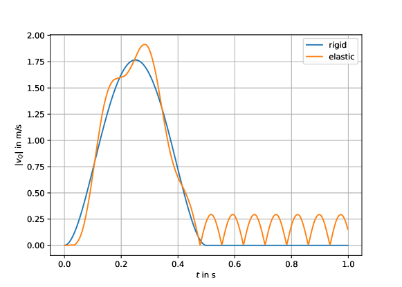
Figure 4: Absolut velocities $|v|$ at the point $Q=(L_{x},0)$ for a rigid body motion (blue) compared to the true elastic motion (orange). Elastic vibrations pertain after the motion of the pivot has been stopped.

Note that the time variation of the angle $\phi(t)$ leads to elastic deformations causing vibrations of the body. Due to lack of a damping mechanism, the vibrations do not fade away when stopping the motion of the pivot at time $t\geq 0.5\,\text{s}$. In the flexible case, a more sophisticated trajectory planning based on the elastic model is needed for the reduction of such structure-induced oscillations, complemented by feedback control, if necessary; see e.g. [41].

As a last step, we would like to illustrate the exact preservation of energy due to the discrete power balance derived in the previous section. To do so, we consider the total energy of the system

$$H_{tot}(v,S,u):=H(v,S)+H_{gra}(u),$$ (26)

consisting of the internal energy $H(v,X)=\frac{1}{2}\langle\rho v,v\rangle_{\Omega}+\frac{1}{2}\langle A:S,S\rangle_{\Omega}$ and the potential energy $H_{gra}(u)=-\langle b,u\rangle_{\Omega}$ due to the graviational forces. The approximation of the total energy in the fully discrete setting is then given by

$$H_{h,tot}^{n}=H(v_{h}^{n},S_{h}^{n})+H_{gra}(\hat{u}_{h}^{n})$$ (27)

with $\hat{u}_{h}^{n}=u_{h}^{n-1/2}+\frac{\tau}{2}v_{h}^{n}=u_{h}^{n+1/2}-\frac{\tau}{2}v_{h}^{n+1}$. With this approximation, the discrete power balance stated in Proposition 3.3 can be rephrased as

$$d_{\tau}H_{h,tot}^{n+1/2}=\langle\lambda_{h}^{n+1/2},v_{D}^{n+1/2}\rangle_{\partial\Omega_{D}}+\langle\tau_{N}^{n+1/2},v_{h}^{n+1/2}\rangle_{\partial\Omega_{N}}.$$ (28)

In our test example, we have $v_{D}=0$ and $\tau_{N}=0$ for all $t\geq 0.5\;\text{s}$. Hence the total energy of the discrete system should be conserved after this time instant. In Figure 5, we display the corresponding results.

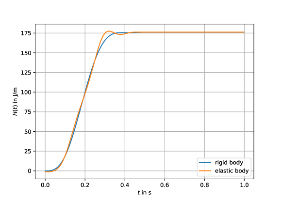
Figure 5: Approximation of the total energy $H_{tot}$ obtained for the rigid body model and the structure-preserving fully discrete approximation of the elasticity system proposed in this paper.

As predicted by our theoretical results, the total energy of the fully discrete systems stays exactly constant after time $t\geq 0.5\;\text{s}$.

5 Discussion

The motion of a geometrically nonlinear elastic continuum was considered by means of a velocity-stress formulation. The governing equations have the form of a PH system in which the skew-symmetric energy-transfer operator is modulated by the displacement field. Based on a weak formulation of the problem, in which the Dirichlet boundary conditions are incorporated by Lagrange multipliers, we derived a power balance and discussed the structure-preserving discretization by mixed finite element methods in space and an implicit midpoint rule in time. A different time integration of the kinematic relation for the displacement field led to a linear implicit time-stepping scheme. The power balance of the system could be proven to be preserved on the semi-discrete and fully-discrete level. The main theoretical results were illustrated by numerical tests for a typical application.

In summary, we obtained a structure-preserving discretization for geometrically nonlinear elastodynamics, which can be realized at the same computational effort as in the linear case. A key step to achieve this was to utilize the PH structure of the velocity-stress formulation, while treating the displacement field as an additional passive kinematic variable. The restriction to St. Venant–Kirchhoff materials used in this paper is suitable for application with large deformation but small strains. The extension to more complex nonlinear energies including multiphysical effects and damping mechanisms is topic of furture research.

References

- [1] C.G. Makridakis, On mixed finite element methods for linear elastodynamics, Numer. Math. 61 (1992), pp. 235–260.
- [2] T. Geveci, On the application of mixed finite element methods to the wave equations, RAIRO Modél. Math. Anal. Numér. 22 (1988), pp. 243–250.
- [3] E. Bécache, P. Joly, and C. Tsogka, A new family of mixed finite elements for the linear elastodynamic problem, SIAM J. Numer. Anal. 39 (2002), pp. 2109–2132.
- [4] G.C. Cohen, Higher-order numerical methods for transient wave equations, Scientific Computation, Springer-Verlag, Berlin, 2002.
- [5] P. Joly, Variational methods for time-dependent wave propagation problems, in Topics in computational wave propagation, Lect. Notes Comput. Sci. Eng. Vol. 31, Springer, Berlin, 2003, pp. 201–264.
- [6] G. Festa and J.P. Vilotte, The Newmark scheme as velocity-stress time-staggering: An efficient PML implementation for spectral element simulations of elastodynamics, Geophys. J. Intl. 161 (2005), pp. 789–812.
- [7] D.N. Arnold and J.J. Lee, Mixed methods for elastodynamics with weak symmetry, SIAM J. Numer. Anal. 52 (2014), pp. 2743–2769.
- [8] G. Scovazzi, T. Song, and X. Zeng, A velocity/stress mixed stabilized nodal finite element for elastodynamics: analysis and computations with strongly and weakly enforced boundary conditions, Comput. Methods Appl. Mech. Engrg. 325 (2017), pp. 532–576.
- [9] B. Zhang, Y. Yang, and M. Feng, Mixed virtual element methods for elastodynamics with weak symmetry, J. Comput. Appl. Math. 353 (2019), pp. 49–71.
- [10] A. Brugnoli, R. Rashad, F. Califano, S. Stramigioli, and D. Matignon, Mixed finite elements for port-Hamiltonian models of von-Kármán beams, IFAC-PapersOnLine 54 (2021), pp. 186–191.
- [11] V. Duindam, A. Macchelli, S. Stramigioli, and H. Bruyninckx (eds.), Modeling and control of complex physical systems, Springer-Verlag, Berlin, 2009.
- [12] B.M. Maschke and A.J. van der Schaft, Port-controlled Hamiltonian systems: modelling origins and systemtheoretic properties, IFAC Proceedings Volumes 25 (1992), pp. 359–365.
- [13] A.J. van der Schaft and B.M. Maschke, Hamiltonian formulation of distributed-parameter systems with boundary energy flow, J. Geom. Phys. 42 (2002), pp. 166–194.
- [14] Y. Le Gorrec, H. Zwart, and B. Maschke, Dirac structures and boundary control systems associated with skew-symmetric differential operators, SIAM J. Control Optim. 44 (2005), pp. 1864–1892.
- [15] A. Macchelli, C. Melchiorri, and S. Stramigioli, Port-based modeling and simulation of mechanical systems with rigid and flexible links, IEEE Trans. Robotics 25 (2009), pp. 1016–1029.
- [16] B. Jacob and H.J. Zwart, Linear port-Hamiltonian systems on infinite-dimensional spaces, Operator Theory: Advances and Applications Vol. 223, Birkhäuser/Springer, Basel, 2012.
- [17] R. Rashad, F. Califano, A.J. van der Schaft, and S. Stramigioli, Twenty years of distributed port-Hamiltonian systems: A literature review, IMA J. Math. Contr. Infor. 37 (2020), pp. 1400–1422.
- [18] G. Golo, V. Talasila, A. van der Schaft, and B. Maschke, Hamiltonian discretization of boundary control systems, Automatica 40 (2004), pp. 757–771.
- [19] O. Farle, D. Klis, M. Jochum, O. Floch, and R. Dyczij-Edlinger, A port-Hamiltonian finite-element formulation for the Maxwell equations, in Proc. of the Int. Conf. on Electromagnetics in Advanced Applications (ICEAA). IEEE, 2013.
- [20] P. Kotyczka, B. Maschke, and L. Lefèvre, Weak form of Stokes-Dirac structures and geometric discretization of port-Hamiltonian systems, J. Comput. Phys. 361 (2018), pp. 442–476.
- [21] F.L. Cardoso-Ribeiro, D. Matignon, and L. Lefèvre, A partitioned finite element method for power-preserving discretization of open systems of conservation laws, IMA J. Math. Control Inform. 38 (2021), pp. 493–533.
- [22] A. Brugnoli, D. Alazard, V. Pommier-Budinger, and D. Matignon, Port-Hamiltonian formulation and symplectic discretization of plate models Part I: Mindlin model for thick plates, Appl. Math. Model. 75 (2019), pp. 940–960.
- [23] A. Brugnoli, D. Alazard, V. Pommier-Budinger, and D. Matignon, Port-Hamiltonian formulation and symplectic discretization of plate models Part II: Kirchhoff model for thin plates, Appl. Math. Model. 75 (2019), pp. 961–981.
- [24] A. Brugnoli, D. Alazard, V. Pommier-Budinger, and D. Matignon, Port-Hamiltonian flexible multibody dynamics, Multibody Syst. Dyn. 51 (2021), pp. 343–375.
- [25] A. Warsewa, M. Böhm, O. Sawodny, and C. Tarín, A port-Hamiltonian approach to modeling the structural dynamics of complex systems, Appl. Math. Model. 89 (2021), pp. 1528–1546.
- [26] A. Brugnoli, D. Alazard, V. Pommier-Budinger, and D. Matignon, A port-Hamiltonian formulation of linear thermoelasticity and its mixed finite element discretization, J. Thermal Stresses 44 (2021), pp. 643–661.
- [27] A. Brugnoli and D. Matignon, A port-Hamiltonian formulation for the full von-Kármán plate model, in 10th European Nonlinear Dynamics Conference (ENOC). 2022.
- [28] T. Thoma and P. Kotyczka, Port-Hamiltonian FE models for filaments, IFAC-PapersOnLine 55 (2022), pp. 353–358.
- [29] P.L. Kinon, T. Thoma, P. Betsch, and P. Kotyczka, Port-Hamiltonian formulation and structure-preserving discretization of hyperelastic strings, in ECCOMAS Thematic Conference on Multibody Dynamics, Lisboa. 2023.
- [30] P. Kotyczka and L. Lefèvre, Discrete-time port-Hamiltonian systems: A definition based on symplectic integration, Systems Contr. Lettr. 133 (2019), p. 104530.
- [31] A. Falaize and T. Hélie, Passive guaranteed simulation of analog audio circuits: a port-Hamiltonian approach, Appl. Sci. 6 (2016), p. 273.
- [32] H. Egger, O. Habrich, and V. Shashkov, On the energy stable approximation of Hamiltonian and gradient systems, Comput. Methods Appl. Math. 21 (2021), pp. 335–349.
- [33] R. Müller, Time-continuous power-balanced simulation of nonlinear audio circuits: realtime processing framework and aliasing rejection, Ph.D. diss., Sorbonne Université, 2021.
- [34] J. Bonet and R.D. Wood, Nonlinear continuum mechanics for finite element analysis, 2nd ed., Cambridge University Press, Cambridge, 2008.
- [35] P. Wriggers, Nonlinear finite element methods, Springer-Verlag, Berlin, 2008.
- [36] V. Mehrmann and B. Unger, Control of port-Hamiltonian differential-algebraic systems and applications, Acta Numer. 32 (2023), pp. 395–515.
- [37] P. Kunkel and V. Mehrmann, Differential-algebraic equations, EMS Textbooks in Mathematics, European Mathematical Society (EMS), Zürich, 2006.
- [38] A. Logg, K.A. Mardal, and G.N. Wells (eds.), Automated solution of differential equations by the finite element method, Lecture Notes in Computational Science and Engineering Vol. 84, Springer, Heidelberg, 2012.
- [39] M. Kuchta, Assembly of multiscale linear PDE operators, in Numerical mathematics and advanced applications—ENUMATH 2019, Lect. Notes Comput. Sci. Eng. Vol. 139, Springer, Cham, 2021, pp. 641–650.
- [40] U. Ayachit, The ParaView guide: Updated for ParaView version 4.3, Kitware, 2015.
- [41] M. Wang and P. Kotyczka, Trajectory control of an elastic beam based on port-Hamiltonian numerical models, at - Automatisierungstechnik 69 (2021), pp. 457–471.