Nesterov Acceleration for Riemannian Optimization

Abstract

In this paper, we generalize the Nesterov accelerated gradient (NAG) method to solve Riemannian optimization problems in a computationally tractable manner. The iteration complexity of our algorithm matches that of the NAG method on the Euclidean space when the objective functions are geodesically convex or geodesically strongly convex. To the best of our knowledge, the proposed algorithm is the first fully accelerated method for geodesically convex optimization problems without requiring strong convexity. Our convergence rate analysis exploits novel metric distortion lemmas as well as carefully designed potential functions. We also identify a connection with the continuous-time dynamics for modeling Riemannian acceleration in Alimisis et al. [1] to understand the accelerated convergence of our scheme through the lens of continuous-time flows.

1 Introduction

We consider Riemannian optimization problems of the form

$$\min_{x\in N\subseteq M}\;f(x),$$ (1.1)

where $M$ is a Riemannian manifold, $N$ is an open geodesically uniquely convex subset of $M$, and $f:N\rightarrow\mathbb{R}$ is a continuously differentiable geodesically convex function. Geodesically convex optimization is the Riemannian version of convex optimization and has salient features such as every local minimum being a global minimum. More interestingly, some (constrained) nonconvex optimization problems defined in the Euclidean space can be considered geodesically convex optimization problems on appropriate Riemannian manifolds [2, Section 1]. Geodesically convex optimization has a wide range of applications, including covariance estimation [3], Gaussian mixture models [4, 5], matrix square root computation [6], metric learning [7], and optimistic likelihood calculation [8]. See [9, Section 1.1] for more examples.

The iteration complexity theory for first-order algorithms is well known when $M=\mathbb{R}^{n}$. Given an initial point $x_{0}$, gradient descent (GD) updates the iterates as

$$x_{k+1}=x_{k}-\gamma_{k}\operatorname{grad}f\left(x_{k}\right).$$ (GD)

For a convex and $L$-smooth objective function $f$, GD with $\gamma_{k}=\frac{1}{L}$ finds an $\epsilon$-approximate solution, i.e., $f\left(x_{k}\right)-f\left(x^{*}\right)\leq\epsilon$, in $O\left(\frac{L}{\epsilon}\right)$ iterations. For a $\mu$-strongly convex and $L$-smooth objective function $f$, GD with $\gamma_{k}=\frac{1}{L}$ finds an $\epsilon$-approximate solution in $O\left(\frac{L}{\mu}\log\frac{L}{\epsilon}\right)$ iterations. A major breakthrough in first-order algorithms is the Nesterov accelerated gradient (NAG) method that achieves a faster convergence rate than GD [10]. Given an initial point $x_{0}=z_{0}$, the NAG scheme updates the iterates as

$$y_{k} =x_{k}+\tau_{k}\left(z_{k}-x_{k}\right)$$ (NAG)

$$x_{k+1} =y_{k}-\alpha_{k}\operatorname{grad}f\left(y_{k}\right)$$

$$z_{k+1} =y_{k}+\beta_{k}\left(z_{k}-y_{k}\right)-\gamma_{k}\operatorname{grad}f\left(y_{k}\right).$$

For a convex and $L$-smooth function $f$, NAG with $\tau_{k}=\frac{2}{k+2}$, $\alpha_{k}=\frac{1}{L}$, $\beta_{k}=1$, $\gamma_{k}=\frac{k+2}{2L}$ (NAG-C) finds an $\epsilon$-approximate solution in $O\left(\sqrt{\frac{L}{\epsilon}}\right)$ iterations [11]. For a $\mu$-strongly convex and $L$-smooth objective function $f$, NAG with $\tau_{k}=\frac{\sqrt{\mu/L}}{1+\sqrt{\mu/L}}$, $\alpha_{k}=\frac{1}{L}$, $\beta_{k}=1-\sqrt{\frac{\mu}{L}}$, $\gamma_{k}=\sqrt{\frac{\mu}{L}}\frac{1}{\mu}$ (NAG-SC) finds an $\epsilon$-approximate solution in $O\left(\sqrt{\frac{L}{\mu}}\log\frac{L}{\epsilon}\right)$ iterations [12].

Considering the problem (1.1) for any Riemannian manifold $M$, [9] successfully generalizes the complexity analysis of GD to Riemannian gradient descent (RGD),

$$x_{k+1}=\exp_{x_{k}}\left(-\gamma_{k}\operatorname{grad}f\left(x_{k}\right)\right),$$ (RGD)

using a lower bound $K_{\min}$ of the sectional curvature and an upper bound $D$ of $\operatorname{diam}(N)$. For completeness, we provide a potential-function analysis in Appendix C to show that RGD with a fixed stepsize has the same iteration complexity as GD.

However, it is still unclear whether a reasonable generalization of NAG to the Riemannian setting is possible with strong theoretical guarantees. When studying the global complexity of Riemannian optimization algorithms, it is common to assume that the sectional curvature of $M$ is bounded below by $K_{\min}$ and bounded above by $K_{\max}$ to prevent the manifold from being overly curved. Unfortunately, [13, 14] show that even when sectional curvature is bounded, achieving global acceleration is impossible in general. Thus, one might need another common assumption, an upper bound $D$ of $\operatorname{diam}(N)$. This motivates our central question:

Can we design computationally tractable accelerated first-order methods on Riemannian manifolds when the sectional curvature and the diameter of the domain are bounded?

In the literature, there are some partial answers but no full answer to this question (see Table 1 and Section 2). In this paper, we provide a complete answer via new first-order algorithms, which we call the Riemannian Nesterov accelerated gradient (RNAG) method. We show that acceleration is possible on Riemannian manifolds for both geodesically convex (g-convex) and geodesically strongly convex (g-strongly convex) cases whenever the bounds $K_{\min}$, $K_{\max}$, and $D$ are available. The main contributions of this work can be summarized as follows:

• Generalizing Nesterov’s scheme, we propose RNAG, a computationally tractable method for Riemannian optimization. We provide two specific algorithms: RNAG-C (Algorithm 1) for minimizing g-convex functions and RNAG-SC (Algorithm 2) for minimizing g-strongly convex functions. Both algorithms call one gradient oracle per iteration. In particular, RNAG-C can be interpreted as a variant of NAG-C with high friction in [15, Section 4.1] (see Remark 1).

• Given the bounds $K_{\min}$, $K_{\max}$, and $D$, we prove that RNAG-C has an $O\left(\sqrt{\frac{L}{\epsilon}}\right)$ iteration complexity (Corollary 1), and that RNAG-SC has an $O\left(\sqrt{\frac{L}{\mu}}\log\frac{L}{\epsilon}\right)$ iteration complexity (Corollary 2). The crucial steps of the proofs are constructing potential functions as (5.2) and handling metric distortion using Lemma 1 and Lemma 2. To our knowledge, this is the first proof for full acceleration in the g-convex case.

• We identify a connection between our algorithms and the ODEs for modeling Riemannian acceleration in [1] by letting the stepsize tend to zero. This analysis confirms the accelerated convergence of our algorithms through the lens of continuous-time flows.

Table 1: Iteration complexities for various accelerated methods on Riemannian manifolds. For the iteration complexity of RAGD [16], $\frac{10}{9}$ is not regarded as a constant because this constant arises from their nonstandard assumption $d\left(x_{0},x^{*}\right)\leq\frac{1}{20\sqrt{\max\left\{K_{\max},-K_{\min}\right\}}}\left(\frac{\mu}{L}\right)^{\frac{3}{4}}$.

Algorithm	Objective function	Iteration complexity	Remark
Algorithm 1 [17]	g-strongly convex	$O\left(\sqrt{L/\mu}\log\left(L/\epsilon\right)\right)$	computationally intractable
Algorithm 2 [17]	g-convex	$O\left(\sqrt{L/\epsilon}\right)$	computationally intractable
RAGD [16]	g-strongly convex	$O\left((10/9)\sqrt{L/\mu}\log\left(L/\epsilon\right)\right)$	nonstandard assumption
RAGDsDR [18]	g-convex	$O\left(\sqrt{\zeta L/\epsilon}\right)$	only in early stages
RNAG-SC (ours)	g-strongly convex	$O\left(\xi\sqrt{L/\mu}\log\left(L/\epsilon\right)\right)$
RNAG-C (ours)	g-convex	$O\left(\xi\sqrt{L/\epsilon}\right)$

2 Related Work

Given a bound $D$ for $\operatorname{diam}(N)$, [17] proposed accelerated methods for both g-convex and g-strongly convex cases. Their algorithms have the same iteration complexities as NAG but require a solution to a nonlinear equation at every iteration, which could be as difficult as solving the original problem in general. Given $K_{\min}$, $K_{\max}$, and $d\left(x_{0},x^{*}\right)$, [16] proposed a computationally tractable algorithm for the g-strongly convex case and showed that their algorithm achieves the iteration complexity $O\left(\frac{10}{9}\sqrt{\frac{L}{\mu}}\log\frac{L}{\epsilon}\right)$ when $d\left(x_{0},x^{*}\right)\leq\frac{1}{20\sqrt{\max\left\{K_{\max},-K_{\min}\right\}}}\left(\frac{\mu}{L}\right)^{\frac{3}{4}}$. Given only $K_{\min}$ and $K_{\max}$, [19] considered the g-strongly convex case. Although full acceleration is not guaranteed, the authors proved that their algorithm eventually achieves acceleration in later stages. Given $K_{\min}$, $K_{\max}$, and $D$, [18] proposed a momentum method for the g-convex case. They showed that their algorithm achieves acceleration in early stages. Although this result is not as strong as full acceleration, their theoretical guarantee is meaningful in practical situations. [20] focused on manifolds with constant sectional curvatures. Their algorithm is accelerated, but it is not straightforward to generalize their argument to any manifolds. Beyond the g-convex setting, [21] studied accelerated methods for nonconvex problems. [22] studied adaptive and momentum-based methods using the trivialization framework in [23]. Further works on accelerated Riemannian optimization can be found in [13, Section 1.6].

Another line of research takes the perspective of continuous-time dynamics as in the Euclidean counterpart [15, 24, 25]. For both g-convex and g-strongly convex cases, [1] proposed ODEs that can model accelerated methods on Riemannian manifolds given $K_{\min}$ and $D$. [26] extended this result and developed a variational framework. Time-discretization methods for such ODEs on Riemannian manifolds have recently been of considerable interest as well [27, 28, 29].

3 Preliminaries

3.1 Background

A Riemannian manifold $(M,g)$ is a real smooth manifold equipped with a Riemannian metric $g$ which assigns to each $p\in M$ a positive-definite inner product $g_{p}(v,w)=\langle v,w\rangle_{p}=\langle v,w\rangle$ on the tangent space $T_{p}M$. The inner product $g_{p}$ induces the norm $\left\|v\right\|_{p}=\|v\|$ defined as $\sqrt{\langle v,v\rangle_{p}}$ on $T_{p}M$. The tangent bundle $TM$ of $M$ is defined as $TM=\sqcup_{p\in M}T_{p}M$. For $p,q\in M$, the geodesic distance $d(p,q)$ between $p$ and $q$ is the infimum of the length of all piecewise continuously differentiable curves from $p$ to $q$. For nonempty set $N\subseteq M$, the diameter $\operatorname{diam}(N)$ of $N$ is defined as $\operatorname{diam}(N)=\sup_{p,q\in N}d(p,q)$.

For a smooth function $f:M\rightarrow\mathbb{R}$, the Riemannian gradient $\operatorname{grad}f(x)$ of $f$ at $x$ is defined as the tangent vector in $T_{x}M$ satisfying

$$\langle\operatorname{grad}f(x),v\rangle=df(x)[v],$$

where $df(x):T_{x}M\rightarrow\mathbb{R}$ is the differential of $f$ at $x$. Let $I:=[0,1]$. A geodesic $\gamma:I\to M$ is a smooth curve of locally minimum length with zero acceleration. In particular, straight lines in $\mathbb{R}^{n}$ are geodesics. The exponential map at $p$ is defined as, for $v\in T_{p}M$,

$$\exp_{p}(v)=\gamma_{v}(1),$$

where $\gamma_{v}:I\rightarrow M$ is the geodesic satisfying $\gamma_{v}(0)=p$ and $\gamma_{v}^{\prime}(0)=v$. In general, $\exp_{p}$ is only defined on a neighborhood of $0$ in $T_{p}M$. It is known that $\exp_{p}$ is a diffeomorphism in some neighborhood $U$ of $0$. Thus, its inverse is well defined and is called the logarithm map $\log_{x}:\exp_{p}(U)\rightarrow T_{p}M$. For a smooth curve $\gamma:I\rightarrow M$ and $t_{0},t_{1}\in I$, the parallel transport $\Gamma(\gamma)_{t_{0}}^{t_{1}}:T_{\gamma(t_{0})}M\rightarrow T_{\gamma(t_{1})}M$ is a way of transporting vectors from $T_{\gamma(t_{0})}M$ to $T_{\gamma(t_{1})}M$ along $\gamma$. When $\gamma$ is a geodesic, we let $\Gamma_{p}^{q}:T_{p}M\rightarrow T_{q}M$ denote the parallel transport from $T_{p}M$ to $T_{q}M$.

A subset $N$ of $M$ is said to be geodesically uniquely convex if for every $x,y\in N$, there exists a unique geodesic $\gamma:[0,1]\rightarrow M$ such that $\gamma(0)=x$, $\gamma(1)=y$, and $\gamma(t)\in N$ for all $t\in[0,1]$. Let $N$ be a geodesically uniquely convex subset of $M$. A function $f:N\rightarrow\mathbb{R}$ is said to be geodesically convex if $f\circ\gamma:[0,1]\rightarrow\mathbb{R}$ is convex for each geodesic $\gamma:[0,1]\rightarrow M$ whose image is in $N$. When $f$ is geodesically convex, we have

$$f(y)\geq f(x)+\left\langle\operatorname{grad}f(x),\log_{x}(y)\right\rangle.$$

Let $N$ be an open geodesically uniquely convex subset of $M$, and $f:N\rightarrow\mathbb{R}$ be a continuously differentiable function. We say that $f$ is geodesically $\mu$-strongly convex for $\mu>0$ if

$$f(y)\geq f(x)+\left\langle\operatorname{grad}f(x),\log_{x}(y)\right\rangle+\frac{\mu}{2}\left\|\log_{x}(y)\right\|^{2}$$

for all $x,y\in N$. We say that $f$ is geodesically $L$-smooth if

$$f(y)\leq f(x)+\left\langle\operatorname{grad}f(x),\log_{x}(y)\right\rangle+\frac{L}{2}\left\|\log_{x}(y)\right\|^{2}$$

for all $x,y\in N$. For additional notions from Riemannian geometry that are used in our analysis, we refer the reader to Appendix A as well as the textbooks [30, 31, 32].

3.2 Assumptions

In this subsection, we present the assumptions that are imposed throughout the paper.

Assumption 1.

The domain $N$ is an open geodesically uniquely convex subset of $M$. The diameter of the domain is bounded as $\mathrm{diam}(N)\leq D<\infty$. The sectional curvature inside $N$ is bounded below by $K_{\min}$ and bounded above by $K_{\max}$. If $K_{\max}>0$, we further assume that $D<\frac{\pi}{\sqrt{K_{\max}}}$.

1 implies that the exponential map $\exp_{x}$ is a diffeomorphism for any $x\in N$ [18].

Assumption 2.

The objective function $f:N\to\mathbb{R}$ is continuously differentiable and geodesically $L$-smooth. Moreover, $f$ is bounded below, and has minimizers, all of which lie in $N$. A global minimizer is denoted by $x^{*}$.

Assumption 3.

All the iterates $x_{k}$ and $y_{k}$ are well-defined on the manifold $M$ remain in $N$.

Although Assumption 3 is common in the literature [16, 19, 18], it is desirable to relax or remove it. We leave the extension as a future research topic.

To implement our algorithms, we also assume that we can compute (or approximate) exponential maps, logarithmic maps, and parallel transport. For many manifolds in practical applications, these maps are implemented in libraries such as [33].

We define the constants $\zeta\geq 1$ and $\delta\leq 1$ as

$$\zeta =\begin{cases}\sqrt{-K_{\min}}D\coth\left(\sqrt{-K_{\min}}D\right),&\text{if }K_{\min}<0\\ 1,&\text{if }K_{\min}\geq 0\end{cases}$$

$$\delta =\begin{cases}1,&\text{if }K_{\max}\leq 0\\ \sqrt{K_{\max}}D\cot\left(\sqrt{K_{\max}}D\right),&\text{if }K_{\max}>0.\end{cases}$$

These constants naturally arise from the Rauch comparison theorem [30, Theorem 11.7] [31, Theorem 6.4.3], and many known methods on Riemannian manifolds have a convergence rate depending on some of these constants [1, 18, 9]. Note that we can set $\zeta=\delta=1$ when $M=\mathbb{R}^{n}$.

4 Algorithms

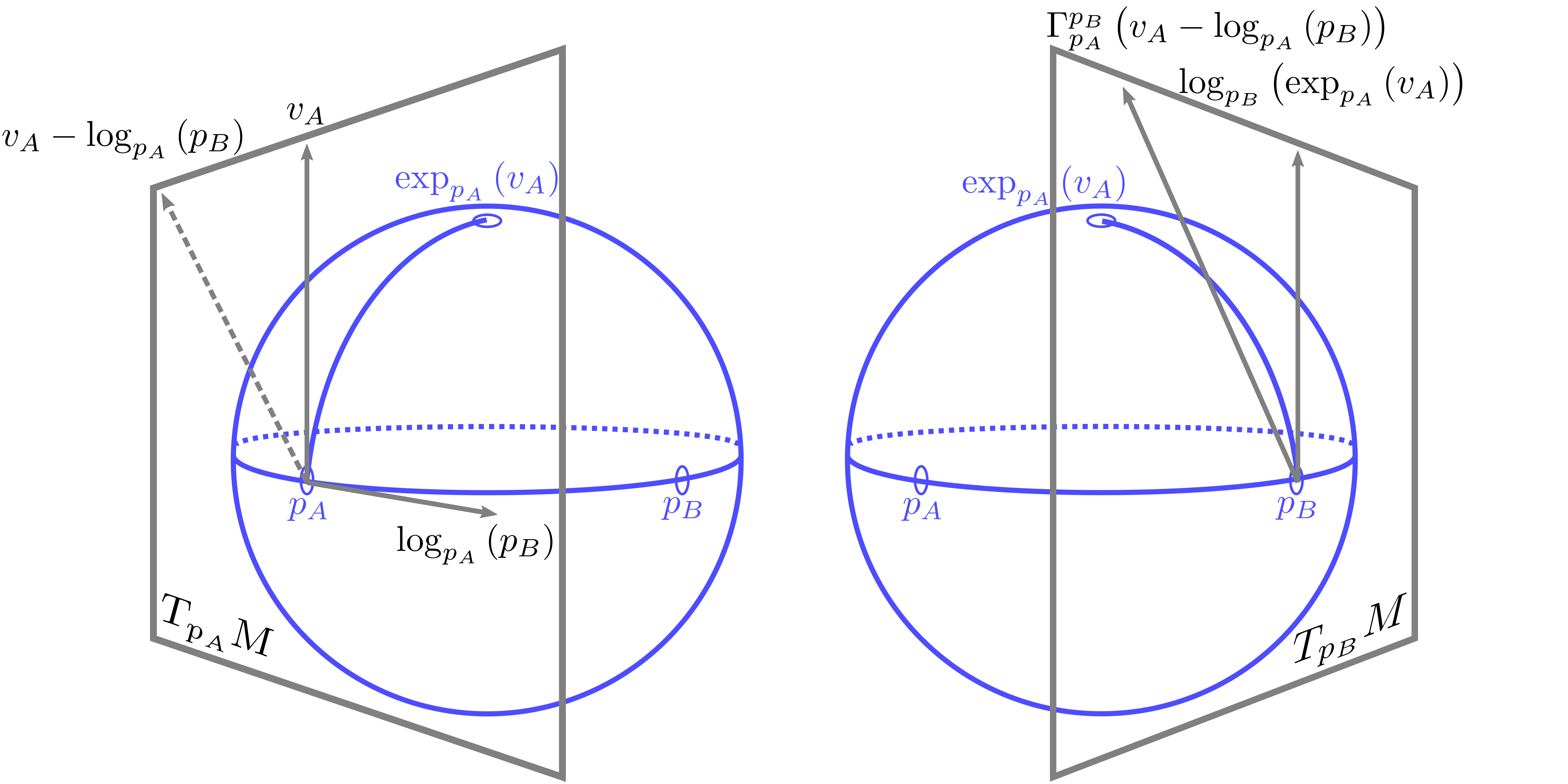
Figure 1: Illustration of the maps $v_{A}\mapsto\Gamma_{p_{A}}^{p_{B}}\left(v_{A}-\log_{p_{A}}\left(p_{B}\right)\right)$ and $v_{A}\mapsto\log_{p_{B}}\left(\exp_{p_{A}}\left(v_{A}\right)\right)$.

In this section, we first generalize Nesterov’s scheme to the Riemannian setting and then design specific algorithms for both g-convex and g-strongly convex cases. In [19, 16] NAG is generalized to a three-step algorithm on a Riemannian manifold as

$$y_{k} =\exp_{x_{k}}\left(\tau_{k}\log_{x_{k}}\left(z_{k}\right)\right)$$ (4.1)

$$x_{k+1} =\exp_{y_{k}}\left(-\alpha_{k}\operatorname{grad}f\left(y_{k}\right)\right)$$

$$z_{k+1} =\exp_{y_{k}}\left(\beta_{k}\log_{y_{k}}\left(z_{k}\right)-\gamma_{k}\operatorname{grad}f\left(y_{k}\right)\right).$$

However, it is more natural to define the iterates $z_{k}$ in the tangent bundle $TM$, instead of in $M$. Thus, we propose another scheme that involves iterates in $TM$ without using $z_{k}$. To associate tangent vectors in different tangent spaces, we use parallel transport, which is a way to transport vectors from one tangent space to another.

  Input: initial point $x_{0}$, parameters $\xi$ and $T>0$, step size $s\leq\frac{1}{L}$

  Initialize $\bar{v}_{0}=0\in T_{x_{0}}M$.

  Set $\lambda_{k}=\frac{k+2\xi+T}{2}$.

  for $k=0$ to $K-1$ do

     $y_{k}=\exp_{x_{k}}\left(\frac{\xi}{\lambda_{k}+\xi-1}\bar{v}_{k}\right)$

     $x_{k+1}=\exp_{y_{k}}\left(-s\operatorname{grad}f\left(y_{k}\right)\right)$

     $v_{k}=\Gamma_{x_{k}}^{y_{k}}\left(\bar{v}_{k}-\log_{x_{k}}\left(y_{k}\right)\right)$

     $\bar{\bar{v}}_{k+1}=v_{k}-\frac{s\lambda_{k}}{\xi}\operatorname{grad}f\left(y_{k}\right)$

     $\bar{v}_{k+1}=\Gamma_{y_{k}}^{x_{k+1}}\left(\bar{\bar{v}}_{k+1}-\log_{y_{k}}\left(x_{k+1}\right)\right)$

  end for

  Output: $x_{K}$

Algorithm 1 RNAG-C

  Input: initial point $x_{0}$, parameter $\xi$, step size $s\leq\frac{1}{L}$

  Initialize $\bar{v}_{0}=0\in T_{x_{0}}M$.

  Set $q=\mu s$.

  for $k=0$ to $K-1$ do

     $y_{k}=\exp_{x_{k}}\left(\frac{\sqrt{\xi q}}{1+\sqrt{\xi q}}\bar{v}_{k}\right)$

     $x_{k+1}=\exp_{y_{k}}\left(-s\operatorname{grad}f\left(y_{k}\right)\right)$

     $v_{k}=\Gamma_{x_{k}}^{y_{k}}\left(\bar{v}_{k}-\log_{x_{k}}\left(y_{k}\right)\right)$

     $\bar{\bar{v}}_{k+1}=\left(1-\sqrt{\frac{q}{\xi}}\right)v_{k}+\sqrt{\frac{q}{\xi}}\left(-\frac{1}{\mu}\operatorname{grad}f\left(y_{k}\right)\right)$

     $\bar{v}_{k+1}=\Gamma_{y_{k}}^{x_{k+1}}\left(\bar{\bar{v}}_{k+1}-\log_{y_{k}}\left(x_{k+1}\right)\right)$

  end for

  Output: $x_{K}$

Algorithm 2 RNAG-SC

Given $z_{k}\in M$ in (4.1), we define the iterates $v_{k}=\log_{y_{k}}\left(z_{k}\right)$, $\bar{v}_{k}=\log_{x_{k}}\left(z_{k}\right)$, and $\bar{\bar{v}}_{k}=\log_{y_{k-1}}\left(z_{k}\right)$ in the tangent bundle $TM$. It is straightforward to check that the following scheme is equivalent to (4.1):

$$y_{k} =\exp_{x_{k}}\left(\tau_{k}\bar{v}_{k}\right)$$ (4.2)

$$x_{k+1} =\exp_{y_{k}}\left(-\alpha_{k}\operatorname{grad}f\left(y_{k}\right)\right)$$

$$v_{k} =\log_{y_{k}}\left(\exp_{x_{k}}\left(\bar{v}_{k}\right)\right)$$

$$\bar{\bar{v}}_{k+1} =\beta_{k}v_{k}-\gamma_{k}\operatorname{grad}f\left(y_{k}\right)$$

$$\bar{v}_{k+1} =\log_{x_{k+1}}\left(\exp_{y_{k}}\left(\bar{\bar{v}}_{k+1}\right)\right).$$

In (4.2), the third and last steps associate tangent vectors in different tangent spaces using the map $T_{p_{A}}M\rightarrow T_{p_{B}}M;\ v_{A}\mapsto\log_{p_{B}}\left(\exp_{p_{A}}\left(v_{A}\right)\right)$. We change these steps by using the map $v_{A}\mapsto\Gamma_{p_{A}}^{p_{B}}\left(v_{A}-\log_{p_{A}}\left(p_{B}\right)\right)$ instead. Technically, this modification allows us to use Lemma 2 when handling metric distortion in our convergence analysis. With the change, we obtain the following scheme, which we call RNAG:

$$y_{k} =\exp_{x_{k}}\left(\tau_{k}\bar{v}_{k}\right)$$ (RNAG)

$$x_{k+1} =\exp_{y_{k}}\left(-\alpha_{k}\operatorname{grad}f\left(y_{k}\right)\right)$$

$$v_{k} =\Gamma_{x_{k}}^{y_{k}}\left(\bar{v}_{k}-\log_{x_{k}}\left(y_{k}\right)\right)$$

$$\bar{\bar{v}}_{k+1} =\beta_{k}v_{k}-\gamma_{k}\operatorname{grad}f\left(y_{k}\right)$$

$$\bar{v}_{k+1} =\Gamma_{y_{k}}^{x_{k+1}}\left(\bar{\bar{v}}_{k+1}-\log_{y_{k}}\left(x_{k+1}\right)\right).$$

Because RNAG only involves exponential maps, logarithm maps, parallel transport, and operations in tangent spaces, this scheme is computationally tractable, unlike the scheme in [17], which involves a nonlinear operator. Note that RNAG is different from the scheme (4.1) because the maps $v_{A}\mapsto\log_{p_{B}}\left(\exp_{p_{A}}\left(v_{A}\right)\right)$ and $v_{A}\mapsto\Gamma_{p_{A}}^{p_{B}}\left(v_{A}-\log_{p_{A}}\left(p_{B}\right)\right)$ are not equivalent in general (see Figure 1).

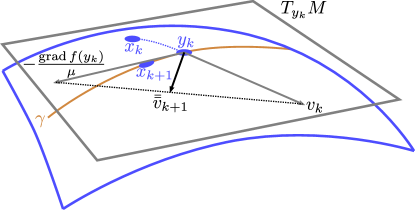
Figure 2: Illustration of RNAG-SC.

By carefully choosing the parameters $\tau_{k}$, $\alpha_{k}$, $\beta_{k}$ and $\gamma_{k}$, we finally obtain two algorithms, RNAG-C (Algorithm 1) for the g-convex case, and RNAG-SC (Algorithm 2) for the g-strongly convex case. In particular, we can interpret RNAG-C as a slight variation of NAG-C with high friction [15, Section 4.1] with the friction parameter $r=1+2\xi$ (see Remark 1). Note that we recover NAG-C and NAG-SC from these algorithms when $M=\mathbb{R}^{n}$ and $\xi=1$. Figure 2 is an illustration of some steps of RNAG-SC, where the curve $\gamma$ is a geodesic with $\gamma(0)=y_{k}$ and $\gamma^{\prime}(0)=\operatorname{grad}f\left(y_{k}\right)$.

5 Convergence Analysis

5.1 Metric distortion lemma

To handle a potential function involving squared norms in tangent spaces, we need to compare distances in different tangent spaces.

Proposition 1.

[1, Lemma 2] Let $\gamma$ be a smooth curve whose image is in $N$. Then, we have

$$\delta\left\|\gamma^{\prime}(t)\right\|^{2}\leq\left\langle D_{t}\log_{\gamma(t)}(x),-\gamma^{\prime}(t)\right\rangle\leq\zeta\left\|\gamma^{\prime}(t)\right\|^{2}.$$

In the proposition above, $D_{t}$ is a covariant derivative along the curve (see Appendix A). Using this proposition, we obtain the following lemma.

Lemma 1.

Let $p_{A},p_{B},x\in N$ and $v_{A}\in T_{p_{A}}M$. If there is $r\in[0,1]$ such that $\log_{p_{A}}\left(p_{B}\right)=rv_{A}$, then we have

$$\left\|v_{B}-\log_{p_{B}}\left(x\right)\right\|_{p_{B}}^{2}+(\zeta-1)\left\|v_{B}\right\|_{p_{B}}^{2}\leq\left\|v_{A}-\log_{p_{A}}\left(x\right)\right\|_{p_{A}}^{2}+(\zeta-1)\left\|v_{A}\right\|_{p_{A}}^{2}.$$

where $v_{B}=\Gamma_{p_{A}}^{p_{B}}\left(v_{A}-\log_{p_{A}}\left(p_{B}\right)\right)\in T_{p_{B}}M$

In particular, when $r=1$, Lemma 1 recovers a weaker version of [9, Lemma 5]. We can further generalize this lemma as follows:

Lemma 2.

Let $p_{A},p_{B},x\in N$ and $v_{A}\in T_{p_{A}}M$. Define $v_{B}=\Gamma_{p_{A}}^{p_{B}}\left(v_{A}-\log_{p_{A}}\left(p_{B}\right)\right)\in T_{p_{B}}M$. If there are $a,b\in T_{p_{A}}M$, and $r\in(0,1)$ such that $v_{A}=a+b$ and $\log_{p_{A}}\left(p_{B}\right)=rb$, then we have

$$\left\|v_{B}-\log_{p_{B}}\left(x\right)\right\|_{p_{B}}^{2}+(\xi-1)\left\|v_{B}\right\|_{p_{B}}^{2}\leq\left\|v_{A}-\log_{p_{A}}\left(x\right)\right\|_{p_{A}}^{2}+(\xi-1)\left\|v_{A}\right\|_{p_{A}}^{2}+\frac{\xi-\delta}{2}\left(\frac{1}{1-r}-1\right)\left\|a\right\|_{p_{A}}^{2}$$

for $\xi\geq\zeta$.

As $\exp_{p_{A}}\left(v_{A}\right)\neq\exp_{p_{B}}\left(v_{B}\right)$ (see Figure 1), our lemma does not compare the projected distance between points on the manifold, unlike [16, Theorem 10] and [19, Lemma 4.1]. The complete proofs of Lemma 1 and Lemma 2 can be found in Appendix B.

5.2 Main results

In this subsection, we analyze the convergence rates of the proposed algorithms. A common way to prove the convergence rate of NAG in Euclidean spaces is showing that the potential function $\phi_{k}$ is decreasing, where $\phi_{k}$ may take the form of

$$\phi_{k}=A_{k}\left(f\left(x_{k}\right)-f\left(x^{*}\right)\right)+B_{k}\left\|z_{k}-x^{*}\right\|^{2}.$$ (5.1)

For the special case $M=\mathbb{R}^{n}$, we provide convergence rate analyses for RNAG-C and RNAG-SC using potential functions of the form (5.1) in Appendix D. To prove the iteration complexities of RNAG-C and RNAG-SC for any manifold $M$, we consider potential functions of the form

$$\phi_{k}=A_{k}\left(f\left(x_{k}\right)-f\left(x^{*}\right)\right)+B_{k}\left(\left\|\bar{v}_{k}-\log_{x_{k}}\left(x^{*}\right)\right\|_{x_{k}}^{2}+(\xi-1)\left\|\bar{v}_{k}\right\|_{x_{k}}^{2}\right).$$ (5.2)

The term $(\xi-1)\left\|\bar{v}_{k}\right\|_{x_{k}}^{2}$ is novel compared with (5.1), and it measures the kinetic energy [24]. Intuitively, this potential makes sense because a large $\xi$ means high friction (see Section 6). This term is useful when handling metric distortion. Our proofs consist of two steps: computation in a tangent space and handling metric distortion.

5.2.1 The geodesically convex case

In the g-convex case, we use a potential function defined as

$$\phi_{k}=s\lambda_{k-1}^{2}\left(f\left(x_{k}\right)-f\left(x^{*}\right)\right)+\frac{\xi}{2}\left\|\bar{v}_{k}-\log_{x_{k}}\left(x^{*}\right)\right\|^{2}+\frac{\xi(\xi-1)}{2}\left\|\bar{v}_{k}\right\|^{2}.$$ (5.3)

The following theorem shows that this potential function is decreasing when $\xi$ and $T$ are chosen appropriately.

Theorem 1.

Let $f$ be a g-convex and geodesically $L$-smooth function. If the parameters $\xi$ and $T$ of RNAG-C satisfy $\xi\geq\zeta$ and

$$\frac{\xi-\delta}{2}\left(\frac{1}{1-\xi/\lambda_{k}}-1\right)\leq(\xi-\zeta)\left(\frac{1}{\left(1-\xi/\left(\lambda_{k}+\xi-1\right)\right)^{2}}-1\right)$$

for all $k\geq 0$, then the iterates of RNAG-C satisfy $\phi_{k+1}\leq\phi_{k}$ for all $k\geq 0$, where $\phi_{k}$ is defined as (5.3).

In particular, we can show that $\xi=\zeta+3(\zeta-\delta)$ and $T=4\xi$ satisfy the condition in Theorem 1. In this case, the monotonicity of the potential function yields

$$f\left(x_{k}\right)-f\left(x^{*}\right)\leq\frac{1}{s\lambda_{k-1}^{2}}\phi_{k}\leq\frac{1}{s\lambda_{k-1}^{2}}\phi_{0}.$$

Thus, we can prove the accelerated convergence rate. The result is summarized in the following corollary.

Corollary 1.

Let $f$ be a g-convex and geodesically $L$-smooth function. Then, RNAG-C with parameters $\xi=\zeta+3(\zeta-\delta)$, $T=4\xi$ and step size $s=\frac{1}{L}$ finds an $\epsilon$-approximate solution in $O\left(\xi\sqrt{\frac{L}{\epsilon}}\right)$ iterations.

This result implies that the iteration complexity of RNAG-C is the same as that of NAG-C because $\xi$ is a constant. The proofs of Theorem 1 and Corollary 1 are contained in Appendix E.

5.2.2 The geodesically strongly convex case

In the g-strongly convex case, we consider a potential function defined as

$$\phi_{k}=\left(1-\sqrt{\frac{q}{\xi}}\right)^{-k}\Biggl{(}f\left(x_{k}\right)-f\left(x^{*}\right)\\ +\frac{\mu}{2}\left\|v_{k}-\log_{y_{k}}\left(x^{*}\right)\right\|^{2}+\frac{\mu(\xi-1)}{2}\left\|v_{k}\right\|^{2}\Biggr{)}.$$ (5.4)

This potential function is also shown to be decreasing under appropriate conditions on $\xi$ and $s$.

Theorem 2.

Let $f$ be a geodesically $\mu$-strongly convex and geodesically $L$-smooth function. If the step size $s$ and the parameter $\xi$ of RNAG-SC satisfy $\xi\geq\zeta$, $\sqrt{\xi q}<1$, and

$$\frac{\xi-\delta}{2}\left(\frac{1}{1-\sqrt{\xi q}}-1\right)\left(1-\sqrt{\frac{q}{\xi}}\right)^{2}-\sqrt{\xi q}\left(1-\sqrt{\frac{q}{\xi}}\right)\leq(\xi-\zeta)\left(\frac{1}{\left(1-\sqrt{\xi q}/\left(1+\sqrt{\xi q}\right)\right)^{2}}-1\right)$$

then the iterates of RNAG-SC satisfy $\phi_{k+1}\leq\phi_{k}$ for all $k\geq 0$, where $\phi_{k}$ is defined as (5.4).

In particular, $\xi=\zeta+3(\zeta-\delta)$ and $s=\frac{1}{9\xi L}$ satisfy the condition in Theorem 2. In this case, by the monotonicity of the potential function, we have

$$f\left(x_{k}\right)-f\left(x^{*}\right)\leq\left(1-\sqrt{\frac{q}{\xi}}\right)^{k}\phi_{k}\leq\left(1-\sqrt{\frac{q}{\xi}}\right)^{k}\phi_{0},$$

which implies that RNAG-SC achieves the accelerated convergence rate. The following corollary summarizes the result.

Corollary 2.

Let $f$ be a geodesically $\mu$-strongly convex and geodesically $L$-smooth function. Then, RNAG-SC with parameter $\xi=\zeta+3(\zeta-\delta)$ and step size $s=\frac{1}{9\xi L}$ finds an $\epsilon$-approximate solution in $O\left(\xi\sqrt{\frac{L}{\mu}}\log\left(\frac{L}{\epsilon}\right)\right)$ iterations.

Because $\xi$ is a constant, the iteration complexity of RNAG-SC is the same as that of NAG-SC. In fact, our linear convergence rate $1-\sqrt{\frac{q}{\xi}}$ is worse than the linear rate $1-\sqrt{q}$ of NAG-SC in the Euclidean space because $\xi\geq 1$ in general. This result matches the linear rate $1-\frac{9}{10}\sqrt{q}$ in [16]. The proofs of Theorem 2 and Corollary 2 can be found in Appendix F.

6 Continuous-Time Interpretation

In this section, we identify a connection to the ODEs for modeling Riemannian acceleration in [1, Equations 2 and 4]. Specifically, following the informal arguments in [15, Section 2] and [34, Section 4.8], we recover the ODEs by taking the limit $s\rightarrow 0$ in our schemes. The detailed analysis is contained in Appendix G. For a sufficiently small $s$, the Euclidean geometry is approximately valid as only a sufficiently small subset of $M$ is considered. Thus, we informally assume $M=\mathbb{R}^{n}$ for simplicity. We can show that the iterations of RNAG-C satisfy

$$\frac{y_{k+1}-y_{k}}{\sqrt{s}} =\frac{\lambda_{k}-1}{\lambda_{k+1}+(\xi-1)}\frac{y_{k}-y_{k-1}}{\sqrt{s}}-\frac{\lambda_{k+1}}{\lambda_{k+1}+(\xi-1)}\sqrt{s}\operatorname{grad}f\left(y_{k}\right)$$

$$\quad+\frac{\lambda_{k}-1}{\lambda_{k+1}+(\xi-1)}\sqrt{s}\left(\operatorname{grad}f\left(y_{k-1}\right)-\operatorname{grad}f\left(y_{k}\right)\right).$$

We introduce a smooth curve $y(t)$ that is approximated by the iterates of RNAG-C as $y(t)\approx y_{t/\sqrt{s}}=y_{k}$ with $k=\frac{t}{\sqrt{s}}$. Using the Taylor expansion, we have

$$\frac{y_{k+1}-y_{k}}{\sqrt{s}} =\dot{y}(t)+\frac{\sqrt{s}}{2}\ddot{y}(t)+o\left(\sqrt{s}\right)$$

$$\frac{y_{k}-y_{k-1}}{\sqrt{s}} =\dot{y}(t)-\frac{\sqrt{s}}{2}\ddot{y}(t)+o\left(\sqrt{s}\right)$$

$$\sqrt{s}\operatorname{grad}f\left(y_{k-1}\right) =\sqrt{s}\operatorname{grad}f\left(y_{k}\right)+o\left(\sqrt{s}\right).$$

Letting $s\rightarrow 0$ yields the ODE

$$\nabla_{\dot{y}}\dot{y}+\frac{1+2\xi}{t}\dot{y}+\operatorname{grad}f(y)=0,$$ (6.1)

where the covariant derivative $\nabla_{\dot{y}}\dot{y}=D_{t}\dot{y}$ is a natural extension of the second derivative $\ddot{y}$ (see Appendix A).

In the g-strongly convex case, we can show that the iterations of RNAG-SC satisfy

$$\frac{y_{k+1}-y_{k}}{\sqrt{s}} =\frac{1-\sqrt{q/\xi}}{1+\sqrt{\xi q}}\frac{y_{k}-y_{k-1}}{\sqrt{s}}-\frac{1+\sqrt{q/\xi}}{1+\sqrt{\xi q}}\sqrt{s}\operatorname{grad}f\left(y_{k}\right)$$

$$\quad+\frac{1-\sqrt{q/\xi}}{1+\sqrt{\xi q}}\sqrt{s}\left(\operatorname{grad}f\left(y_{k-1}\right)-\operatorname{grad}f\left(y_{k}\right)\right).$$

Through a similar limiting process, we obtain the following ODE:

$$\nabla_{\dot{y}}\dot{y}+\left(\frac{1}{\sqrt{\xi}}+\sqrt{\xi}\right)\sqrt{\mu}\dot{y}+\operatorname{grad}f(y)=0.$$ (6.2)

Note that replacing the parameter $\xi$ in the coefficients of our ODEs with $\zeta$ recovers [1, Equations 2 and 4]. Because $\xi\geq\zeta$, the continuous-time acceleration results [1, Theorems 5 and 7] are valid for our ODEs as well. Thus, this analysis confirms the accelerated convergence of our algorithms through the lens of continuous-time flows.

In both ODEs, the parameter $\xi\geq\zeta$ appears in the coefficient of the friction term $\dot{X}$, increasing with $\xi$. Intuitively, this makes sense because $\zeta$ is large for an ill-conditioned domain, where $-K_{\min}$ and $D$ are large and thus metric distortion is more severe (where one might want to decrease the effect of momentum).

7 Experiments

In this section, we examine the performance of our algorithms on the Rayleigh quotient maximization problem and the Karcher mean problem. To implement the geometry of manifolds, we use the Python libraries Pymanopt [33] and Geomstats [35]. For comparison, we use the known accelerated algorithms RAGD [16] for the g-strongly convex case and RNAGsDR with no line search [18] for the g-convex case. To implement these algorithms, we reuse the code in [18].

We set the input parameters $\zeta=1$ for implementing RAGDsDR, and $\xi=1$ for implementing our algorithms. The stepsize is chosen as $s=\frac{1}{L}$ in our algorithms.

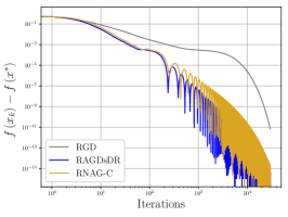
(a) Rayleigh quotient maximization

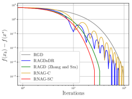
(b) Karcher mean of SPD matrices

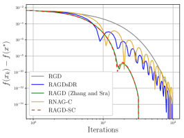
(c) Karcher mean on hyperbolic space

Figure 3: Performances of various Riemannian optimization algorithms on the Rayleigh quotient maximization problem and the Karcher mean problem.

Rayleigh quotient maximization. Given a real $d\times d$ symmetric matrix $A$, we consider the problem

$$\min_{x\in\mathbb{S}^{d-1}}f(x)=-\frac{1}{2}x^{\top}Ax.$$

on the unit $(d-1)$-sphere on $\mathbb{S}^{d-1}$. For this manifold, we can set $K_{\min}=K_{\max}=1$. We set $d=1000$ and $A=\frac{1}{2}\left(B+B^{\top}\right)$, where the entries of $B\in\mathbb{R}^{d\times d}$ are randomly generated by the Gaussian distribution $N(0,1/d)$. We have the smoothness parameter $L=\lambda_{\max}-\lambda_{\min}$ by the following proposition.

Proposition 2.

The function $f$ is geodesically $\left(\lambda_{\max}-\lambda_{\min}\right)$-smooth, where $\lambda_{\max}$ and $\lambda_{\min}$ are the largest and smallest eigenvalues of $A$, respectively.

The proof can be found in Appendix H. The result is shown in Figure 3(a). We observe that RNAG-C perform better than RGD and similar to RAGDsDR, which is a known accelerated method for the g-convex case.

Karcher mean of SPD matrices. When $K_{\max}\leq 0$, the Karcher mean [36] of the points $p_{i}\in M$ for $i=1,\ldots,n$, is defined as the solution of

$$\min_{x\in M}f(x)=\frac{1}{2n}\sum_{i=1}^{n}d\left(x,p_{i}\right)^{2}.$$ (7.1)

The following proposition gives the strong convexity parameter $\mu=1$.

Proposition 3.

The function $f$ is geodesically $1$-strongly convex.

The proof can be found in Appendix H. We consider this problem on the manifold of symmetric positive definite matrices $\mathcal{P}(d)\subseteq\mathbb{R}^{d\times d}$ endowed with the Riemannian metric $\langle X,Y\rangle_{P}=\operatorname{Tr}\left(P^{-1}XP^{-1}Y\right)$. It is known that one can set $K_{\min}=-\frac{1}{2}$ and $K_{\max}=0$ [21, Appendix I]. We set $d=100$ and $n=50$. The matrices $p_{i}$ are randomly generated using Matrix Mean Toolbox [37] with condition number ${10}^{6}$, which can be also found in the code of [18]. We set the smoothness parameter as $L=10$. The result is shown in Figure 3(b). We observe that RNAG-SC and RAGD (Zhang and Sra) perform significantly better than RGD. The performances of RNAG-C and RAGDsDR are only slightly better than that of RGD in early stages. This makes sense because $f$ is g-strongly convex and well-conditioned.

Karcher mean on hyperbolic space. We consider the problem (7.1) on the hyperbolic space $\mathbb{H}^{d}$ with the hyperboloid model $\mathbb{H}^{d}=\left\{x\in\mathbb{R}^{d+1}:-x_{d+1}^{2}+\sum_{k=1}^{d}x_{k}^{2}=-1\right\}$. For this manifold, we can set $K_{\min}=K_{\max}=-1$. We set $d=1000$ and $n=10$. First $d$ entries of each point $p_{i}$ are randomly generated by the Gaussian distribution $N(0,1/d)$. We set the smoothness parameter as $L=10$. The result is similar to the previous example, and shown in Figure 3(c).

8 Conclusions

In this paper, we have proposed novel computationally tractable first-order methods that achieve Riemannian acceleration for both g-convex and g-strongly convex objective functions whenever the constants $K_{\min}$, $K_{\max}$, and $D$ are available. The iteration complexities of RNAG-C and RNAG-SC match those of their Euclidean counterparts. The continuous-time analysis of our algorithms provides an intuitive interpretation of the parameter $\xi$ as a measurement of friction, which is higher when the domain manifold is more ill-conditioned.

In fact, the iteration complexities of our algorithms depend on the parameter $\xi\geq\zeta$, which is affected by the values of the constants $K_{\min}$, $K_{\max}$, and $D$. When $\zeta$ is large (i.e., $-K_{\min}$ and $D$ are large), we have a worse guarantee. A possible future direction is to study the effect of the constants $K_{\min}$, $K_{\max}$, and $D$ on the complexities of Riemannian optimization algorithms tightly.

Appendix A Background

Definition 1.

A smooth vector field $V$ is a smooth map from $M$ to $TM$ such that $p\circ V$ is the identity map, where $p:TM\rightarrow M$ is the projection. The collection of all smooth vector fields on $M$ is denoted by $\mathfrak{X}(M)$.

Definition 2.

Let $\gamma:I\rightarrow M$ be a smooth curve. A smooth vector field $V$ along $\gamma$ is a smooth map from $I$ to $TM$ such that $V(t)\in T_{\gamma(t)}M$ for all $t\in I$. The collection of all smooth vector fields along $\gamma$ is denoted by $\mathfrak{X}(\gamma)$.

Proposition 4 (Fundamental theorem of Riemannian geometry).

There exists a unique operator

$$\nabla:\mathfrak{X}(M)\times\mathfrak{X}(M)\rightarrow\mathfrak{X}(M):\ (U,V)\mapsto\nabla_{U}V$$

satisfying the following properties for any $U,V,W\in\mathfrak{X}(M)$, smooth functions $f,g$ on $M$, and $a,b\in\mathbb{R}$:

1. $\nabla_{fU+gW}V=f\nabla_{U}V+g\nabla_{W}V$

2. $\nabla_{U}(aV+bW)=a\nabla_{U}V+b\nabla_{U}W$

3. $\nabla_{U}(fV)=(Uf)V+f\nabla_{U}V$

4. $[U,V]=\nabla_{U}V-\nabla_{V}U$

5. $U\langle V,W\rangle=\langle\nabla_{U}V,W\rangle+\langle V,\nabla_{U}W\rangle$,

where $[\cdot,\cdot]$ denotes the Lie bracket. The operator $\nabla$ is called the Levi-Civita connection or the Riemannian connection. The field $\nabla_{U}V$ is called the covariant derivative of $V$ along $U$.

From now on, we always assume that $M$ is equipped with the Riemannian connection $\nabla$.

Proposition 5.

[32, Section 8.11] For any smooth vector fields $U,V$ on $M$, the vector field $\nabla_{U}V$ at $x$ depends on $U$ only through $U(x)$. Thus, we can write $\nabla_{u}V$ to mean $(\nabla_{U}V)(x)$ for any $U\in\mathfrak{X}(M)$ such that $U(x)=u$, without ambiguity.

For a smooth function $f:M\rightarrow\mathbb{R}$, $\operatorname{grad}f$ is a smooth vector field.

Definition 3.

[32, Section 8.11] The Riemannian Hessian of a smooth function $f$ on $M$ at $x\in M$ is a self-adjoint linear operator $\operatorname{Hess}f(x):T_{x}M\rightarrow T_{x}M$ defined as

$$\operatorname{Hess}f(x)[u]=\nabla_{u}\operatorname{grad}f.$$

Proposition 6.

[32, Section 8.12] Let $c:I\rightarrow M$ be a smooth curve. There exists a unique operator $D_{t}:\mathfrak{X}(c)\rightarrow\mathfrak{X}(c)$ satisfying the following properties for all $Y,Z\in\mathfrak{X}(c)$, $U\in\mathfrak{X}(M)$, a smooth function $g$ on $I$, and $a,b\in\mathbb{R}$:

1. $D_{t}(aY+bZ)=aD_{t}Y+bD_{t}Z$

2. $D_{t}(gZ)=g^{\prime}Z+gD_{t}Z$

3. $(D_{t}(U\circ c))(t)=\nabla_{c^{\prime}(t)}U$ for all $t\in I$

4. $\frac{d}{dt}\langle Y,Z\rangle=\langle D_{t}Y,Z\rangle+\langle Y,D_{t}Z\rangle$.

This operator is called the (induced) covariant derivative along the curve $c$.

We define the acceleration of a smooth curve $\gamma$ as the vector field $D_{t}\gamma^{\prime}$ along $\gamma$. Now, we can define the parallel transport using covariant derivatives.

Definition 4.

[32, Section 10.3] A vector field $Z\in\mathfrak{X}(c)$ is parallel if $D_{t}Z=0$.

Proposition 7.

[32, Section 10.3] For any smooth curve $c:I\rightarrow M$, $t_{0}\in I$ and $u\in T_{c(t_{0})}M$, there exists a unique parallel vector field $Z\in\mathfrak{X}(c)$ such that $Z(t_{0})=u$.

Definition 5.

[32, Section 10.3] Given a smooth curve $c$ on $M$, the parallel transport of tangent vectors at $c(t_{0})$ to the tangent space at $c(t_{1})$ along $c$,

$$\Gamma(c)_{t_{0}}^{t_{1}}:T_{c(t_{0})}M\rightarrow T_{c(t_{1})}M,$$

is defined by $\Gamma(c)_{t_{0}}^{t_{1}}(u)=Z(t_{1})$, where $Z\in\mathfrak{X}(c)$ is the unique parallel vector field such that $Z(t_{0})=u$.

Proposition 8.

[32, Section 10.3] The parallel transport operator $\Gamma(c)_{t_{0}}^{t_{1}}$ is linear. Also, $\Gamma(c)_{t_{1}}^{t_{2}}\circ\Gamma(c)_{t_{0}}^{t_{1}}=\Gamma(c)_{t_{0}}^{t_{2}}$ and $\Gamma(c)_{t}^{t}$ is the identity. In particular, the inverse of $\Gamma(c)_{t_{0}}^{t_{1}}$ is $\Gamma(c)_{t_{1}}^{t_{0}}$. The parallel transport is an isometry, that is,

$$\langle u,v\rangle_{c\left(t_{0}\right)}=\left\langle\Gamma(c)_{t_{0}}^{t_{1}}(u),\Gamma(c)_{t_{0}}^{t_{1}}(v)\right\rangle_{c\left(t_{1}\right)}.$$

Proposition 9.

[32, Section 10.3] Consider a smooth curve $c:I\rightarrow M$. Given a vector field $Z\in\mathfrak{X}(c)$, we have

$$D_{t}Z(t)=\lim_{h\rightarrow 0}\frac{\Gamma(c)_{t+h}^{t}Z(t+h)-Z(t)}{h}.$$

Appendix B Proofs of Lemma 1 and Lemma 2

Proposition 10.

[1, Lemma 12] Let $\gamma$ be a smooth curve whose image is in $N$, then

$$\frac{d}{dt}\left\|\log_{\gamma(t)}(x)\right\|^{2}=2\left\langle D_{t}\log_{\gamma(t)}(x),\log_{\gamma(t)}(x)\right\rangle=2\left\langle\log_{\gamma(t)}(x),-\gamma^{\prime}(t)\right\rangle.$$

See 1

Proof.

By geodesic unique convexity of $N$, there is a unique geodesic $\gamma$ such that $\gamma(0)=p_{A}$ and $\gamma(r)=p_{B}$ whose image lies in $N$. We can check that $\gamma^{\prime}(0)=v_{A}$. Define the vector field $V(t)$ along $\gamma$ as $V(t)=\Gamma(\gamma)_{0}^{t}\left(v_{A}-t\gamma^{\prime}(0)\right)$. Then, we can check that $V(t)=(1-t)\gamma^{\prime}(t)$ and $V^{\prime}(t)=-\gamma^{\prime}(t)$. Define the function $w:[0,r]\rightarrow\mathbb{R}$ as $w(t)=\left\|\log_{\gamma(t)}(x)-V(t)\right\|^{2}$, It follows from Proposition 1 and Proposition 10 that

$$\frac{d}{dt}w(t) =2\left\langle D_{t}\left(\log_{\gamma(t)}(x)-V(t)\right),\log_{\gamma(t)}(x)-V(t)\right\rangle$$

$$=2\left\langle D_{t}\log_{\gamma(t)}(x),\log_{\gamma(t)}(x)\right\rangle-2\left\langle D_{t}\log_{\gamma(t)}(x),V(t)\right\rangle-2\left\langle D_{t}V(t),\log_{\gamma(t)}(x)\right\rangle+2\left\langle D_{t}V(t),V(t)\right\rangle$$

$$=2\left\langle D_{t}\log_{\gamma(t)}(x),\log_{\gamma(t)}(x)\right\rangle-2(1-t)\left\langle D_{t}\log_{\gamma(t)}(x),\gamma^{\prime}(t)\right\rangle+2\left\langle\gamma^{\prime}(t),\log_{\gamma(t)}(x)\right\rangle+2\left\langle D_{t}V(t),V(t)\right\rangle$$

$$=2(1-t)\left\langle D_{t}\log_{\gamma(t)}(x),-\gamma^{\prime}(t)\right\rangle+2\left\langle D_{t}V(t),V(t)\right\rangle$$

$$\leq 2(1-t)\zeta\left\|\gamma^{\prime}(t)\right\|^{2}+2\left\langle D_{t}V(t),V(t)\right\rangle$$

$$=-2\zeta\left\langle-\gamma^{\prime}(t),(1-t)\gamma^{\prime}(t)\right\rangle+2\left\langle D_{t}V(t),V(t)\right\rangle$$

$$=-2(\zeta-1)\left\langle D_{t}V(t),V(t)\right\rangle$$

$$=-(\zeta-1)\left(\frac{d}{dt}\left\|V(t)\right\|^{2}\right).$$

Integrating both sides from $0$ to $r$ gives

$$w(r)-w(0)\leq\int_{0}^{r}-(\zeta-1)\left(\frac{d}{dt}\left\|V(t)\right\|^{2}\right)\,dt=-(\zeta-1)\left(\left\|V(r)\right\|^{2}-\left\|V(0)\right\|^{2}\right).$$

This completes the proof. ∎

See 2

Proof.

Define $\gamma$, $V$, $w$ as in the proof of Lemma 1. As in the proof of Lemma 1, we can check that $\gamma^{\prime}(0)=b$ and $V^{\prime}(t)=-\gamma^{\prime}(t)$, and that we have

$$\frac{d}{dt}w(t)=-2\left\langle D_{t}\log_{\gamma(t)}(x),V(t)\right\rangle+2\left\langle D_{t}V(t),V(t)\right\rangle.$$

Consider the smooth function $f_{0}:p\mapsto\frac{1}{2}\left\|\log_{p}(x)\right\|^{2}$. Because $\operatorname{grad}f_{0}(p)=-\log_{p}(x)$, we have $\operatorname{Hess}f_{0}(\gamma(t))[w]=\nabla_{w}X$, where $X:p\mapsto-\log_{p}(x)$ [1, Section 4]. By Proposition 1, we have $\delta\left\|w\right\|^{2}\leq\left\langle\operatorname{Hess}f_{0}(\gamma(t))[w],w\right\rangle\leq\zeta\left\|w\right\|^{2}\leq\xi\left\|w\right\|^{2}$ [18, Appendix D]. Thus,

$$-\frac{\xi-\delta}{2}\left\|w\right\|^{2}=\delta\left\|w\right\|^{2}-\frac{\xi+\delta}{2}\left\|w\right\|^{2}\leq\left\langle\operatorname{Hess}f_{0}(\gamma(t))[w]-\frac{\xi+\delta}{2}w,w\right\rangle\leq\xi\left\|w\right\|^{2}-\frac{\xi+\delta}{2}\left\|w\right\|^{2}=\frac{\xi-\delta}{2}\left\|w\right\|^{2}.$$

Because $\operatorname{Hess}f_{0}(\gamma(t))$ is self-adjoint, it is diagonalizable. Thus, the norm of the operator $\operatorname{Hess}f_{0}(\gamma(t))-\frac{\xi+\delta}{2}I$ on $T_{\gamma(t)}M$ can be bounded as

$$\left\|\operatorname{Hess}f_{0}(\gamma(t))-\frac{\xi+\delta}{2}I\right\|\leq\frac{\xi-\delta}{2}.$$

Now, we have

$$-2\left\langle D_{t}\log_{\gamma(t)}(x),V(t)\right\rangle =2\left\langle\nabla_{\gamma^{\prime}(t)}X,V(t)\right\rangle$$

$$=2\left\langle\operatorname{Hess}f_{0}(\gamma(t))[\gamma^{\prime}(t)],V(t)\right\rangle$$

$$=2\left\langle\left(\operatorname{Hess}f_{0}(\gamma(t))-\frac{\xi+\delta}{2}I\right)\left(\gamma^{\prime}(t)\right),V(t)\right\rangle+2\left\langle\frac{\xi+\delta}{2}\gamma^{\prime}(t),V(t)\right\rangle$$

$$\leq 2\left\|\left(\operatorname{Hess}f_{0}(\gamma(t))-\frac{\xi+\delta}{2}I\right)\left(\gamma^{\prime}(t)\right)\right\|\left\|V(t)\right\|+2\left\langle\frac{\xi+\delta}{2}\gamma^{\prime}(t),V(t)\right\rangle$$

$$\leq 2\left\|\operatorname{Hess}f_{0}(\gamma(t))-\frac{\xi+\delta}{2}I\right\|\left\|\gamma^{\prime}(t)\right\|\left\|V(t)\right\|+2\left\langle\frac{\xi+\delta}{2}\gamma^{\prime}(t),V(t)\right\rangle$$

$$\leq 2\frac{\xi-\delta}{2}\left\|\gamma^{\prime}(t)\right\|\left\|V(t)\right\|+2\left\langle\frac{\xi+\delta}{2}\gamma^{\prime}(t),V(t)\right\rangle.$$

Because the parallel transport preserves inner product and norm, we obtain

$$-2\left\langle D_{t}\log_{\gamma(t)}(x),V(t)\right\rangle \leq 2\frac{\xi-\delta}{2}\left\|b\right\|\left\|a+(1-t)b\right\|+(\xi+\delta)\left\langle b,a+(1-t)b\right\rangle$$

$$=\frac{\xi-\delta}{2}\frac{1}{1-t}2\left\|(1-t)b\right\|\left\|a+(1-t)b\right\|+(\xi+\delta)\left\langle b,a+(1-t)b\right\rangle$$

$$\leq\frac{\xi-\delta}{2}\frac{1}{1-t}\left(\left\|(1-t)b\right\|^{2}+\left\|a+(1-t)b\right\|^{2}\right)+(\xi+\delta)\left\langle b,a+(1-t)b\right\rangle$$

$$=\frac{\xi-\delta}{2}\frac{1}{1-t}\left\|a\right\|^{2}-2\xi\left\langle-b,a+(1-t)b\right\rangle$$

$$=\frac{\xi-\delta}{2}\frac{1}{1-t}\left\|a\right\|^{2}-2\xi\left\langle D_{t}V(t),V(t)\right\rangle.$$

Thus, for $t\in(0,r)$

$$\frac{d}{dt}w(t)\leq\frac{\xi-\delta}{2}\frac{1}{1-r}\left\|a\right\|^{2}-2(\xi-1)\left\langle D_{t}V(t),V(t)\right\rangle.$$

Integrating both sides from $0$ to $r$, the result follows. ∎

Appendix C Convergence Analysis for RGD

In this section, we review the iteration complexity of RGD with the fixed step size $\gamma_{k}=s$ under the assumptions in Section 3.2. The results in this section correspond to [9, Theorems 13 and 15].

C.1 Geodesically convex case

We define the potential function as

$$\phi_{k}=s(k+\zeta-1)\left(f\left(x_{k}\right)-f\left(x^{*}\right)\right)+\frac{1}{2}\left\|\log_{x_{k}}\left(x^{*}\right)\right\|^{2}.$$

The following theorem says that $\phi_{k}$ is decreasing.

Theorem 3.

Let $f$ be a geodesically convex and geodesically $L$-smooth function. If $s\leq\frac{1}{L}$, then the iterates of RGD satisfy

$$s(k+\zeta)\left(f\left(x_{k+1}\right)-f\left(x^{*}\right)\right)+\frac{1}{2}\left\|\log_{x_{k+1}}\left(x^{*}\right)\right\|^{2}\leq s(k+\zeta-1)\left(f\left(x_{k}\right)-f\left(x^{*}\right)\right)+\frac{1}{2}\left\|\log_{x_{k}}\left(x^{*}\right)\right\|^{2}$$

for all $k\geq 0$.

Proof.

(Step 1). In this step, $\langle\cdot,\cdot\rangle$ and $\|\cdot\|$ always denote the inner product and the norm on $T_{x_{k}}M$. It follows from the geodesic convexity of $f$ that

$$f\left(x^{*}\right) \geq f\left(x_{k}\right)+\left\langle\operatorname{grad}f\left(x_{k}\right),\log_{x_{k}}\left(x^{*}\right)\right\rangle$$

$$=f\left(x_{k}\right)-\frac{1}{s}\left\langle\log_{x_{k}}\left(x_{k+1}\right),\log_{x_{k}}\left(x^{*}\right)\right\rangle.$$

By the geodesic $\frac{1}{s}$-smoothness of $f$, we have

$$f\left(x_{k+1}\right) \leq f\left(x_{k}\right)+\left\langle\operatorname{grad}f\left(x_{k}\right),\log_{x_{k}}\left(x_{k+1}\right)\right\rangle+\frac{1}{2s}\left\|\log_{x_{k}}\left(x_{k+1}\right)\right\|^{2}$$

$$=f\left(x_{k}\right)-\frac{1}{2s}\left\|\log_{x_{k}}\left(x_{k+1}\right)\right\|^{2}.$$

Taking a weighted sum of these inequalities yields

$$0 \geq\left[f\left(x_{k}\right)-f\left(x^{*}\right)-\frac{1}{s}\left\langle\log_{x_{k}}\left(x_{k+1}\right),\log_{x_{k}}\left(x^{*}\right)\right\rangle\right]$$

$$\quad+(k+\zeta)\left[f\left(x_{k+1}\right)-f\left(x_{k}\right)+\frac{1}{2s}\left\|\log_{x_{k}}\left(x_{k+1}\right)\right\|^{2}\right]$$

$$=(k+\zeta)\left(f\left(x_{k+1}\right)-f\left(x^{*}\right)\right)-(k+\zeta-1)\left(f\left(x_{k}\right)-f\left(x^{*}\right)\right)$$

$$\quad-\frac{1}{s}\left\langle\log_{x_{k}}\left(x_{k+1}\right),\log_{x_{k}}\left(x^{*}\right)\right\rangle+\frac{k+\zeta}{2s}\left\|\log_{x_{k}}\left(x_{k+1}\right)\right\|^{2}$$

$$\geq(k+\zeta)\left(f\left(x_{k+1}\right)-f\left(x^{*}\right)\right)-(k+\zeta-1)\left(f\left(x_{k}\right)-f\left(x^{*}\right)\right)$$

$$\quad-\frac{1}{s}\left\langle\log_{x_{k}}\left(x_{k+1}\right),\log_{x_{k}}\left(x^{*}\right)\right\rangle+\frac{\zeta}{2s}\left\|\log_{x_{k}}\left(x_{k+1}\right)\right\|^{2}$$

$$=(k+\zeta)\left(f\left(x_{k+1}\right)-f\left(x^{*}\right)\right)-(k+\zeta-1)\left(f\left(x_{k}\right)-f\left(x^{*}\right)\right)$$

$$\quad+\frac{1}{2s}\left(\zeta\left\|\log_{x_{k}}\left(x_{k+1}\right)\right\|^{2}-2\left\langle\log_{x_{k}}\left(x_{k+1}\right),\log_{x_{k}}\left(x^{*}\right)\right\rangle\right)$$

$$=(k+\zeta)\left(f\left(x_{k+1}\right)-f\left(x^{*}\right)\right)-(k+\zeta-1)\left(f\left(x_{k}\right)-f\left(x^{*}\right)\right)$$

$$\quad+\frac{1}{2s}\left(\left\|\log_{x_{k}}\left(x_{k+1}\right)-\log_{x_{k}}\left(x^{*}\right)\right\|^{2}+(\zeta-1)\left\|\log_{x_{k}}\left(x_{k+1}\right)\right\|^{2}-\left\|\log_{x_{k}}\left(x^{*}\right)\right\|^{2}\right).$$

(Step 2: Handling metric distortion). By Lemma 1 with $p_{A}=x_{k}$, $p_{B}=x_{k+1}$, $x=x^{*}$, $v_{A}=\log_{x_{k}}\left(x_{k+1}\right)$, $v_{B}=0$, $r=1$, we have

$$\left\|\log_{x_{k+1}}\left(x^{*}\right)\right\|_{x_{k+1}}^{2}\leq\left\|\log_{x_{k}}\left(x_{k+1}\right)-\log_{x_{k}}\left(x^{*}\right)\right\|_{x_{k}}^{2}+(\zeta-1)\left\|\log_{x_{k}}\left(x_{k+1}\right)\right\|_{x_{k}}^{2}.$$

Combining this inequality with the result in Step 1 gives

$$0 \geq(k+\zeta)\left(f\left(x_{k+1}\right)-f\left(x^{*}\right)\right)-(k+\zeta-1)\left(f\left(x_{k}\right)-f\left(x^{*}\right)\right)$$

$$\quad+\frac{1}{2s}\left(\left\|\log_{x_{k}}\left(x_{k+1}\right)-\log_{x_{k}}\left(x^{*}\right)\right\|_{x_{k}}^{2}+(\zeta-1)\left\|\log_{x_{k}}\left(x_{k+1}\right)\right\|_{x_{k}}^{2}-\left\|\log_{x_{k}}\left(x^{*}\right)\right\|_{x_{k}}^{2}\right)$$

$$\quad+\frac{1}{2s}\left(\left\|\log_{x_{k+1}}\left(x^{*}\right)\right\|_{x_{k+1}}^{2}-\left\|\log_{x_{k}}\left(x_{k+1}\right)-\log_{x_{k}}\left(x^{*}\right)\right\|_{x_{k}}^{2}-(\zeta-1)\left\|\log_{x_{k}}\left(x_{k+1}\right)\right\|_{x_{k}}^{2}\right)$$

$$=(k+\zeta)\left(f\left(x_{k+1}\right)-f\left(x^{*}\right)\right)-(k+\zeta-1)\left(f\left(x_{k}\right)-f\left(x^{*}\right)\right)+\frac{1}{2s}\left\|\log_{x_{k+1}}\left(x^{*}\right)\right\|_{x_{k+1}}^{2}-\frac{1}{2s}\left\|\log_{x_{k}}\left(x^{*}\right)\right\|_{x_{k}}^{2}$$

$$=\frac{\phi_{k+1}-\phi_{k}}{s}.$$

∎

Corollary 3.

Let $f$ be a geodesically convex and geodesically $L$-smooth function. Then, RGD with the step size $s=\frac{1}{L}$ finds an $\epsilon$-approximate solution in $O\left(\frac{\zeta L}{\epsilon}\right)$ iterations.

Proof.

It follows from Theorem 3 that

$$f\left(x_{k}\right)-f\left(x^{*}\right)\leq\frac{\phi_{k}}{s(k+\zeta-1)}\leq\frac{\phi_{0}}{s(k+\zeta-1)}=\frac{1}{s(k+\zeta-1)}\left(s(\zeta-1)\left(f\left(x_{0}\right)-f\left(x^{*}\right)\right)+\frac{1}{2}\left\|\log_{x_{0}}\left(x^{*}\right)\right\|^{2}\right).$$

By geodesic $\frac{1}{s}$-smoothness of $f$, we have

$$f\left(x_{k}\right)-f\left(x^{*}\right)\leq\frac{1}{s(k+\zeta-1)}\left(s(\zeta-1)\frac{1}{2s}\left\|\log_{x_{0}}\left(x^{*}\right)\right\|^{2}+\frac{1}{2}\left\|\log_{x_{0}}\left(x^{*}\right)\right\|^{2}\right)=\frac{\zeta L}{2(k+\zeta-1)}\left\|\log_{x_{0}}\left(x^{*}\right)\right\|^{2}.$$

Thus, we have $f\left(x_{k}\right)-f\left(x^{*}\right)\leq\epsilon$ whenever $k\geq\frac{\zeta L}{2\epsilon}\left\|\log_{x_{0}}\left(x^{*}\right)\right\|^{2}-(\zeta-1)$. Thus we obtain an $O\left(\frac{\zeta L}{\epsilon}\right)$ iteration complexity. ∎

This result implies that the iteration complexity of RGD for geodesically convex case is the same as that of GD, since $\zeta$ is a constant.

C.2 Geodesically strongly convex case

We define the potential function as

$$\phi_{k}=(1-\mu s)^{-k}\left(f\left(x_{k}\right)-f\left(x^{*}\right)+\frac{\mu}{2}\left\|\log_{x_{k}}\left(x^{*}\right)\right\|^{2}\right).$$

The following theorem states that $\phi_{k}$ is decreasing.

Theorem 4.

Let $f$ be a geodesically $\mu$-strongly convex and geodesically $L$-smooth function. If $s\leq\min\left\{\frac{1}{L},\frac{1}{\zeta\mu}\right\}$, then the iterates of RGD satisfy

$$(1-\mu s)^{-(k+1)}\left(f\left(x_{k+1}\right)-f\left(x^{*}\right)+\frac{\mu}{2}\left\|\log_{x_{k+1}}\left(x^{*}\right)\right\|^{2}\right)\leq(1-\mu s)^{-k}\left(f\left(x_{k}\right)-f\left(x^{*}\right)+\frac{\mu}{2}\left\|\log_{x_{k}}\left(x^{*}\right)\right\|^{2}\right)$$

for all $k\geq 0$.

Proof.

(Step 1). In this step, $\langle\cdot,\cdot\rangle$ and $\|\cdot\|$ always denote the inner product and the norm on $T_{x_{k}}M$. Set $q=\mu s$. By geodesic $\mu$-strong convexity of $f$, we have

$$f\left(x^{*}\right) \geq f\left(x_{k}\right)+\left\langle\operatorname{grad}f\left(x_{k}\right),\log_{x_{k}}\left(x^{*}\right)\right\rangle+\frac{\mu}{2}\left\|\log_{x_{k}}\left(x^{*}\right)\right\|^{2}$$

$$=f\left(x_{k}\right)-\frac{1}{s}\left\langle\log_{x_{k}}\left(x_{k+1}\right),\log_{x_{k}}\left(x^{*}\right)\right\rangle+\frac{q}{2s}\left\|\log_{x_{k}}\left(x^{*}\right)\right\|^{2}.$$

By geodesic $\frac{1}{s}$-smoothness of $f$, we have

$$f\left(x_{k+1}\right) \leq f\left(x_{k}\right)+\left\langle\operatorname{grad}f\left(x_{k}\right),\log_{x_{k}}\left(x_{k+1}\right)\right\rangle+\frac{1}{2s}\left\|\log_{x_{k}}\left(x_{k+1}\right)\right\|^{2}$$

$$=f\left(x_{k}\right)-\frac{1}{2s}\left\|\log_{x_{k}}\left(x_{k+1}\right)\right\|^{2}.$$

Note that $\zeta q\leq 1$. Taking weighted sum of these inequalities, we arrive to the valid inequality

$$0 \geq q\left[f\left(x_{k}\right)-f\left(x^{*}\right)-\frac{1}{s}\left\langle\log_{x_{k}}\left(x_{k+1}\right),\log_{x_{k}}\left(x^{*}\right)\right\rangle+\frac{q}{2s}\left\|\log_{x_{k}}\left(x^{*}\right)\right\|^{2}.\right]$$

$$\quad+\left[f\left(x_{k+1}\right)-f\left(x_{k}\right)+\frac{1}{2s}\left\|\log_{x_{k}}\left(x_{k+1}\right)\right\|^{2}\right]$$

$$=f\left(x_{k+1}\right)-f\left(x^{*}\right)-(1-q)\left(f\left(x_{k}\right)-f\left(x^{*}\right)\right)$$

$$\quad-\frac{q}{s}\left\langle\log_{x_{k}}\left(x_{k+1}\right),\log_{x_{k}}\left(x^{*}\right)\right\rangle+\frac{q^{2}}{2s}\left\|\log_{x_{k}}\left(x^{*}\right)\right\|^{2}+\frac{1}{2s}\left\|\log_{x_{k}}\left(x_{k+1}\right)\right\|^{2}$$

$$\geq f\left(x_{k+1}\right)-f\left(x^{*}\right)-(1-q)\left(f\left(x_{k}\right)-f\left(x^{*}\right)\right)$$

$$\quad+\frac{q}{2s}\left(-2\left\langle\log_{x_{k}}\left(x_{k+1}\right),\log_{x_{k}}\left(x^{*}\right)\right\rangle+q\left\|\log_{x_{k}}\left(x^{*}\right)\right\|^{2}+\zeta\left\|\log_{x_{k}}\left(x_{k+1}\right)\right\|^{2}\right)$$

$$=f\left(x_{k+1}\right)-f\left(x^{*}\right)-(1-q)\left(f\left(x_{k}\right)-f\left(x^{*}\right)\right)$$

$$\quad+\frac{q}{2s}\left(\left\|\log_{x_{k}}\left(x_{k+1}\right)-\log_{x_{k}}\left(x^{*}\right)\right\|^{2}+(\zeta-1)\left\|\log_{x_{k}}\left(x_{k+1}\right)\right\|^{2}-(1-q)\left\|\log_{x_{k}}\left(x^{*}\right)\right\|^{2}\right).$$

(Step 2: Handle metric distortion). By Lemma 1 with $p_{A}=x_{k}$, $p_{B}=x_{k+1}$, $x=x^{*}$, $v_{A}=\log_{x_{k}}\left(x_{k+1}\right)$, $v_{B}=0$, $r=1$, we have

$$\left\|\log_{x_{k+1}}\left(x^{*}\right)\right\|_{x_{k+1}}^{2}\leq\left\|\log_{x_{k}}\left(x_{k+1}\right)-\log_{x_{k}}\left(x^{*}\right)\right\|_{x_{k}}^{2}+(\zeta-1)\left\|\log_{x_{k}}\left(x_{k+1}\right)\right\|_{x_{k}}^{2}.$$

Combining this inequality with the result in Step 1 gives

$$0 \geq f\left(x_{k+1}\right)-f\left(x^{*}\right)-(1-q)\left(f\left(x_{k}\right)-f\left(x^{*}\right)\right)$$

$$\quad+\frac{q}{2s}\left(\left\|\log_{x_{k}}\left(x_{k+1}\right)-\log_{x_{k}}\left(x^{*}\right)\right\|_{x_{k}}^{2}+(\zeta-1)\left\|\log_{x_{k}}\left(x_{k+1}\right)\right\|_{x_{k}}^{2}-(1-q)\left\|\log_{x_{k}}\left(x^{*}\right)\right\|_{x_{k}}^{2}\right)$$

$$\quad+\frac{q}{2s}\left(\left\|\log_{x_{k+1}}\left(x^{*}\right)\right\|_{x_{k+1}}^{2}-\left\|\log_{x_{k}}\left(x_{k+1}\right)-\log_{x_{k}}\left(x^{*}\right)\right\|_{x_{k}}^{2}-(\zeta-1)\left\|\log_{x_{k}}\left(x_{k+1}\right)\right\|_{x_{k}}^{2}\right)$$

$$0 =f\left(x_{k+1}\right)-f\left(x^{*}\right)-(1-q)\left(f\left(x_{k}\right)-f\left(x^{*}\right)\right)+\frac{q}{2s}\left\|\log_{x_{k+!}}\left(x^{*}\right)\right\|_{x_{k+1}}^{2}-\frac{q}{2s}(1-q)\left\|\log_{x_{k}}\left(x^{*}\right)\right\|_{x_{k}}^{2}$$

$$=\left(f\left(x_{k+1}\right)-f\left(x^{*}\right)+\frac{\mu}{2}\left\|\log_{x_{k+1}}\left(x^{*}\right)\right\|_{x_{k+1}}^{2}\right)-(1-q)\left(f\left(x_{k}\right)-f\left(x^{*}\right)+\frac{\mu}{2}\left\|\log_{x_{k}}\left(x^{*}\right)\right\|_{x_{k}}^{2}\right)$$

$$=(1-q)^{(k+1)}\left(\phi_{k+1}-\phi_{k}\right).$$

∎

Corollary 4.

Let $f$ be a geodesically $\mu$-strongly convex and geodesically $L$-smooth function. Then, RGD with step size $s=\frac{1}{\zeta L}$ finds an $\epsilon$-approximate solution in $O\left(\frac{\zeta L}{\mu}\log\frac{L}{\epsilon}\right)$ iterations.

Proof.

By Theorem 4, we have

$$f\left(x_{k}\right)-f\left(x^{*}\right)\leq\left(1-\mu s\right)^{k}\phi_{k}\leq\left(1-\mu s\right)^{k}\phi_{0}=\left(1-\mu s\right)^{k}\left(f\left(x_{0}\right)-f\left(x^{*}\right)+\frac{\mu}{2}\left\|\log_{x_{0}}\left(x^{*}\right)\right\|^{2}\right).$$

It follows from the geodesic $L$-smoothness of $f$ and the inequality $\left(1-\frac{\mu}{\zeta L}\right)^{k}\leq e^{-\frac{\mu}{\zeta L}k}$ that

$$f\left(x_{k}\right)-f\left(x^{*}\right)\leq\left(1-\frac{\mu}{\zeta L}\right)^{k}\left(\frac{L}{2}\left\|\log_{x_{0}}\left(x^{*}\right)\right\|^{2}+\frac{\mu}{2}\left\|\log_{x_{0}}\left(x^{*}\right)\right\|^{2}\right)\leq e^{-\frac{\mu}{\zeta L}k}L\left\|\log_{x_{0}}\left(x^{*}\right)\right\|^{2}.$$

Thus, we have $f\left(x_{k}\right)-f\left(x^{*}\right)\leq\epsilon$ whenever $k\geq\frac{\zeta L}{\mu}\log\left(\frac{L}{\epsilon}\left\|\log_{x_{0}}\left(x^{*}\right)\right\|^{2}\right)$. Accordingly, we obtain an $O\left(\frac{\zeta L}{\mu}\log\frac{L}{\epsilon}\right)$ iteration complexity. ∎

This result implies that the iteration complexity of RGD for g-strongly convex case is the same as that of GD, since $\zeta$ is a constant. Another proof of the iteration complexity of RGD for g-strongly convex functions can be found in [13, Proposition 1.8].

Appendix D RNAG-C and RNAG-SC on the Euclidean space

In this section, we give simpler analyses for the convergence of RNAG-C and RNAG-SC on the Euclidean space, using potential functions of the form (5.1).

D.1 The convex case

Under the identification $z_{k}=\exp_{y_{k}}\left(v_{k}\right)$, we can write the updating rule of RNAG-C as

$$y_{k} =x_{k}+\frac{\xi}{\lambda_{k}+\xi-1}\left(z_{k}-x_{k}\right)$$ (RNAG-C)

$$x_{k+1} =y_{k}-s\operatorname{grad}f\left(y_{k}\right)$$

$$z_{k+1} =z_{k}-\frac{s\lambda_{k}}{\xi}\operatorname{grad}f\left(y_{k}\right),$$

where $\lambda_{k}=\frac{k+2\xi+T}{2}$. We consider a potential function defined as

$$\phi_{k}=s\lambda_{k-1}^{2}\left(f\left(x_{k}\right)-f\left(x^{*}\right)\right)+\frac{\xi^{2}}{2}\left\|z_{k}-x^{*}\right\|^{2}.$$ (D.1)

The following theorem shows that this potential function can be used to prove the convergence rate of RNAG-C.

Theorem 5.

Let $f$ be a convex and $L$-smooth function on $\mathbb{R}^{n}$. Then, the iterates of RNAG-C satisfy $\phi_{k+1}\leq\phi_{k}$ for all $k\geq 0$, where $\phi_{k}$ is defined as (D.1).

Proof.

It is easy to check that $\operatorname{grad}f\left(y_{k}\right)=-\frac{\xi}{s\lambda_{k}}\left(z_{k+1}-z_{k}\right)$, $x_{k}-y_{k}=-\frac{\xi}{\lambda_{k}-1}\left(z_{k}-y_{k}\right)$, and $\lambda_{k}^{2}-\lambda_{k}\leq\lambda_{k-1}^{2}$. By convexity of $f$, we have

$$f\left(x^{*}\right) \geq f\left(y_{k}\right)+\left\langle\operatorname{grad}f\left(y_{k}\right),x^{*}-y_{k}\right\rangle$$

$$=f\left(y_{k}\right)-\frac{\xi}{s\lambda_{k}}\left\langle z_{k+1}-z_{k},x^{*}-y_{k}\right\rangle,$$

$$f\left(x_{k}\right) \geq f\left(y_{k}\right)+\left\langle\operatorname{grad}f\left(y_{k}\right),x_{k}-y_{k}\right\rangle$$

$$=f\left(y_{k}\right)+\frac{\xi^{2}}{s\left(\lambda_{k}^{2}-\lambda_{k}\right)}\left\langle z_{k+1}-z_{k},z_{k}-y_{k}\right\rangle.$$

It follows from $\frac{1}{s}$-smoothness of $f$ that

$$f\left(x_{k+1}\right) \leq f\left(y_{k}\right)+\left\langle\operatorname{grad}f\left(y_{k}\right),x_{k+1}-y_{k}\right\rangle+\frac{1}{2s}\left\|x_{k+1}-y_{k}\right\|^{2}$$

$$=f\left(y_{k}\right)-\frac{s}{2}\left\|\operatorname{grad}f\left(y_{k}\right)\right\|^{2}$$

$$=f\left(y_{k}\right)-\frac{\xi^{2}}{2s\lambda_{k}^{2}}\left\|z_{k+1}-z_{k}\right\|^{2}.$$

Taking a weighted sum of these inequalities yields

$$0 \geq\xi\lambda_{k}\left[f\left(y_{k}\right)-f\left(x^{*}\right)-\frac{\xi}{s\lambda_{k}}\left\langle z_{k+1}-z_{k},x^{*}-y_{k}\right\rangle,\right]$$

$$\quad+\left(\lambda_{k}^{2}-\lambda_{k}\right)\left[f\left(y_{k}\right)-f\left(x_{k}\right)+\frac{\xi^{2}}{s\left(\lambda_{k}^{2}-\lambda_{k}\right)}\left\langle z_{k+1}-z_{k},z_{k}-y_{k}\right\rangle.\right]$$

$$\quad+\lambda_{k}^{2}\left[f\left(x_{k+1}\right)-f\left(y_{k}\right)+\frac{\xi^{2}}{2s\lambda_{k}^{2}}\left\|z_{k+1}-z_{k}\right\|^{2}\right]$$

$$=\lambda_{k}^{2}\left(f\left(x_{k+1}\right)-f\left(x^{*}\right)\right)-\left(\lambda_{k}^{2}-\lambda_{k}\right)\left(f\left(x_{k}\right)-f\left(x^{*}\right)\right)+(\xi-1)\lambda_{k}\left(f\left(y_{k}\right)-f\left(x^{*}\right)\right)$$

$$\quad-\frac{\xi^{2}}{s}\left\langle z_{k+1}-z_{k},x^{*}-y_{k}\right\rangle+\frac{\xi^{2}}{s}\left\langle z_{k+1}-z_{k},z_{k}-y_{k}\right\rangle+\frac{\xi^{2}}{2s}\left\|z_{k+1}-z_{k}\right\|^{2}$$

$$\geq\lambda_{k}^{2}\left(f\left(x_{k+1}\right)-f\left(x^{*}\right)\right)-\lambda_{k-1}^{2}\left(f\left(x_{k}\right)-f\left(x^{*}\right)\right)$$

$$\quad+\frac{\xi^{2}}{2s}\left(-2\left\langle z_{k+1}-z_{k},x^{*}-y_{k}\right\rangle+2\left\langle z_{k+1}-z_{k},z_{k}-y_{k}\right\rangle+\left\|z_{k+1}-z_{k}\right\|^{2}\right)$$

$$=\lambda_{k}^{2}\left(f\left(x_{k+1}\right)-f\left(x^{*}\right)\right)-\lambda_{k-1}^{2}\left(f\left(x_{k}\right)-f\left(x^{*}\right)\right)$$

$$\quad+\frac{\xi^{2}}{2s}\left(\left\|z_{k+1}-z_{k}\right\|^{2}-2\left\langle z_{k+1}-z_{k},x^{*}-z_{k}\right\rangle\right).$$

Note that

$$\left\|z_{k+1}-x^{*}\right\|^{2}-\left\|z_{k}-x^{*}\right\|^{2}=\left\|z_{k+1}-z_{k}\right\|^{2}-2\left\langle z_{k+1}-z_{k},x^{*}-z_{k}\right\rangle.$$

Thus, we obtain

$$0 \geq\lambda_{k}^{2}\left(f\left(x_{k+1}\right)-f\left(x^{*}\right)\right)-\lambda_{k-1}^{2}\left(f\left(x_{k}\right)-f\left(x^{*}\right)\right)+\frac{\xi^{2}}{2s}\left(\left\|z_{k+1}-x^{*}\right\|^{2}-\left\|z_{k}-x^{*}\right\|^{2}\right)$$

$$=\frac{\phi_{k+1}-\phi_{k}}{s}.$$

∎

Remark 1 (Comparison with high-friction NAG-C).

In [15, Section 4.1], high-friction NAG-C is proposed as

$$x_{k} =y_{k-1}-s\operatorname{grad}f\left(y_{k-1}\right)$$

$$y_{k} =x_{k}+\frac{k-1}{k+r-1}\left(x_{k}-x_{k-1}\right).$$

Introducing the third sequence as $z_{k}=y_{k}+\frac{k}{r-1}\left(y_{k}-x_{k}\right)$, we can rewrite this method as

$$y_{k} =x_{k}+\frac{r-1}{k+r-1}\left(z_{k}-x_{k}\right)$$ (NAG-C-HF)

$$x_{k+1} =y_{k}-s\operatorname{grad}f\left(y_{k}\right)$$

$$z_{k+1} =z_{k}-\frac{k+r-1}{r-1}s\operatorname{grad}f\left(y_{k}\right).$$

One can see that NAG-C-HF with $r=1+2\xi$ is similar to RNAG-C, where the only difference occurs in constants that can be ignored as $k$ grows.

D.2 The strongly convex case

Under the identification $z_{k}=\exp_{y_{k}}\left(v_{k}\right)$, we can write the updating rule of RNAG-SC as

$$y_{k} =x_{k}+\frac{\sqrt{\xi q}}{1+\sqrt{\xi q}}\left(z_{k}-x_{k}\right)$$ (RNAG-SC)

$$x_{k+1} =y_{k}-s\operatorname{grad}f\left(y_{k}\right)$$

$$z_{k+1} =\left(1-\sqrt{\frac{q}{\xi}}\right)z_{k}+\sqrt{\frac{q}{\xi}}\left(-\frac{1}{\mu}\operatorname{grad}f\left(y_{k}\right)\right),$$

where $q=\mu s$. We consider a potential function defined as

$$\phi_{k}=\left(1-\sqrt{\frac{q}{\xi}}\right)^{-k}\left(f\left(x_{k}\right)-f\left(x^{*}\right)+\frac{\xi\mu}{2}\left\|z_{k}-x^{*}\right\|^{2}\right).$$ (D.2)

The following theorem shows that this potential function can be used to prove the convergence rate of RNAG-SC.

Theorem 6.

Let $f$ be a $\mu$-strongly convex and $L$-smooth function on $\mathbb{R}^{n}$. Then, the iterates of RNAG-SC satisfy $\phi_{k+1}\leq\phi_{k}$ for all $k\geq 0$, where $\phi_{k}$ is defined as(D.2).

Proof.

It is straightforward to check that $\operatorname{grad}f\left(y_{k}\right)=\mu\frac{1-\sqrt{q/\xi}}{\sqrt{q/\xi}}\left(z_{k}-y_{k}\right)-\mu\frac{1}{\sqrt{q/\xi}}\left(z_{k+1}-y_{k}\right)$ and $x_{k}-y_{k}=-\sqrt{\xi q}\left(z_{k}-y_{k}\right)$. By $\mu$-strong convexity of $f$, we have

$$f\left(x^{*}\right) \geq f\left(y_{k}\right)+\left\langle\operatorname{grad}f\left(y_{k}\right),x^{*}-y_{k}\right\rangle+\frac{\mu}{2}\left\|x^{*}-y_{k}\right\|^{2}$$

$$=f\left(y_{k}\right)+\mu\frac{1-\sqrt{q/\xi}}{\sqrt{q/\xi}}\left\langle z_{k}-y_{k},x^{*}-y_{k}\right\rangle-\mu\frac{1}{\sqrt{q/\xi}}\left\langle z_{k+1}-y_{k},x^{*}-y_{k}\right\rangle+\frac{\mu}{2}\left\|x^{*}-y_{k}\right\|^{2}.$$

It follows from convexity of $f$ that

$$f\left(x_{k}\right) \geq f\left(y_{k}\right)+\left\langle\operatorname{grad}f\left(y_{k}\right),x_{k}-y_{k}\right\rangle$$

$$=f\left(y_{k}\right)-\xi\mu\left(1-\sqrt{\frac{q}{\xi}}\right)\left\|z_{k}-y_{k}\right\|^{2}+\xi\mu\left\langle z_{k}-y_{k},z_{k+1}-y_{k}\right\rangle.$$

By $\frac{1}{s}$-smoothness of $f$, we have

$$f\left(x_{k+1}\right) \leq f\left(y_{k}\right)+\left\langle\operatorname{grad}f\left(y_{k}\right),x_{k+1}-y_{k}\right\rangle+\frac{1}{2s}\left\|x_{k+1}-y_{k}\right\|^{2}$$

$$=f\left(y_{k}\right)-\frac{s}{2}\left\|\operatorname{grad}f\left(y_{k}\right)\right\|^{2}$$

$$=f\left(y_{k}\right)-\frac{s}{2}\left\|\mu\frac{1-\sqrt{q/\xi}}{\sqrt{q/\xi}}z_{k}-\mu\frac{1}{\sqrt{q/\xi}}z_{k+1}\right\|^{2}$$

$$=f\left(y_{k}\right)-\frac{\xi\mu}{2}\left(1-\sqrt{\frac{q}{\xi}}\right)^{2}\left\|z_{k}-y_{k}\right\|^{2}+\xi\mu\left(1-\sqrt{\frac{q}{\xi}}\right)\left\langle z_{k}-y_{k},z_{k+1}-y_{k}\right\rangle-\frac{\xi\mu}{2}\left\|z_{k+1}-y_{k}\right\|^{2}.$$

Taking a weighted sum of these inequalities yields

$$0 \geq\sqrt{\xi q}\left[f\left(y_{k}\right)-f\left(x^{*}\right)+\mu\frac{1-\sqrt{q/\xi}}{\sqrt{q/\xi}}\left\langle z_{k}-y_{k},x^{*}-y_{k}\right\rangle-\mu\frac{1}{\sqrt{q/\xi}}\left\langle z_{k+1}-y_{k},x^{*}-y_{k}\right\rangle+\frac{\mu}{2}\left\|x^{*}-y_{k}\right\|^{2}\right]$$

$$\quad+\left(1-\sqrt{\frac{q}{\xi}}\right)\left[f\left(y_{k}\right)-f\left(x_{k}\right)-\xi\mu\left(1-\sqrt{\frac{q}{\xi}}\right)\left\|z_{k}-y_{k}\right\|^{2}+\xi\mu\left\langle z_{k}-y_{k},z_{k+1}-y_{k}\right\rangle\right]$$

$$\quad+\left[f\left(x_{k+1}\right)-f\left(y_{k}\right)+\frac{\xi\mu}{2}\left(1-\sqrt{\frac{q}{\xi}}\right)^{2}\left\|z_{k}-y_{k}\right\|^{2}-\xi\mu\left(1-\sqrt{\frac{q}{\xi}}\right)\left\langle z_{k}-y_{k},z_{k+1}-y_{k}\right\rangle+\frac{\xi\mu}{2}\left\|z_{k+1}-y_{k}\right\|^{2}\right]$$

$$=\left(f\left(x_{k+1}\right)-f\left(x^{*}\right)\right)-\left(1-\sqrt{\frac{q}{\xi}}\right)\left(f\left(x_{k}\right)-f\left(x^{*}\right)\right)+\left(\sqrt{\xi}-\frac{1}{\sqrt{\xi}}\right)\sqrt{q}\left(f\left(y_{k}\right)-f\left(x^{*}\right)\right)$$

$$\quad+\xi\mu\left(1-\sqrt{\frac{q}{\xi}}\right)\left\langle z_{k}-y_{k},x^{*}-y_{k}\right\rangle-\xi\mu\left\langle z_{k+1}-y_{k},x^{*}-y_{k}\right\rangle+\frac{\xi\mu}{2}\sqrt{\frac{q}{\xi}}\left\|x^{*}-y_{k}\right\|^{2}$$

$$\quad-\frac{\xi\mu}{2}\left(1-\sqrt{\frac{q}{\xi}}\right)^{2}\left\|z_{k}-y_{k}\right\|^{2}+\frac{\xi\mu}{2}\left\|z_{k+1}-y_{k}\right\|^{2}.$$

We further notice that

$$\left\|z_{k+1}-x^{*}\right\|^{2}-\left(1-\sqrt{\frac{q}{\xi}}\right)\left\|z_{k}-x^{*}\right\|^{2}$$

$$=\left\|\left(z_{k+1}-y_{k}\right)-\left(x^{*}-y_{k}\right)\right\|^{2}-\left(1-\sqrt{\frac{q}{\xi}}\right)\left\|\left(z_{k}-y_{k}\right)-\left(x^{*}-y_{k}\right)\right\|^{2}$$

$$=\left\|z_{k+1}-y_{k}\right\|^{2}-2\left\langle z_{k+1}-y_{k},x^{*}-y_{k}\right\rangle-\left(1-\sqrt{\frac{q}{\xi}}\right)\left\|z_{k}-y_{k}\right\|^{2}$$

$$\quad+2\left(1-\sqrt{\frac{q}{\xi}}\right)\left\langle z_{k}-y_{k},x^{*}-y_{k}\right\rangle+\sqrt{\frac{q}{\xi}}\left\|x^{*}-y_{k}\right\|^{2}.$$

Therefore, we obtain

$$0 \geq\left(f\left(x_{k+1}\right)-f\left(x^{*}\right)+\frac{\xi\mu}{2}\left\|\bar{\bar{v}}_{k+1}-\log_{y_{k}}\left(x^{*}\right)\right\|^{2}\right)-\left(1-\sqrt{\frac{q}{\xi}}\right)\left(f\left(x_{k}\right)-f\left(x^{*}\right)+\frac{\xi\mu}{2}\left\|v_{k}-\log_{y_{k}}\left(x^{*}\right)\right\|^{2}\right)$$

$$\quad+\left(\sqrt{\xi}-\frac{1}{\sqrt{\xi}}\right)\sqrt{q}\left(f\left(y_{k}\right)-f\left(x^{*}\right)\right)+\frac{\xi\mu}{2}\sqrt{\frac{q}{\xi}}\left(1-\sqrt{\frac{q}{\xi}}\right)\left\|z_{k}-y_{k}\right\|^{2}$$

$$\geq\left(f\left(x_{k+1}\right)-f\left(x^{*}\right)+\frac{\xi\mu}{2}\left\|\bar{\bar{v}}_{k+1}-\log_{y_{k}}\left(x^{*}\right)\right\|^{2}\right)-\left(1-\sqrt{\frac{q}{\xi}}\right)\left(f\left(x_{k}\right)-f\left(x^{*}\right)+\frac{\xi\mu}{2}\left\|v_{k}-\log_{y_{k}}\left(x^{*}\right)\right\|^{2}\right)$$

$$=\left(1-\sqrt{\frac{q}{\xi}}\right)^{k+1}\left(\phi_{k+1}-\phi_{k}\right).$$

∎

Appendix E Convergence Analysis for RNAG-C

See 1

Proof.

(Step 1). In this step, $\langle\cdot,\cdot\rangle$ and $\|\cdot\|$ always denote the inner product and the norm on $T_{y_{k}}M$. It is easy to check that $\operatorname{grad}f\left(y_{k}\right)=-\frac{\xi}{s\lambda_{k}}\left(\bar{\bar{v}}_{k+1}-v_{k}\right)$, $\log_{y_{k}}\left(x_{k}\right)=-\frac{\xi}{\lambda_{k}-1}v_{k}$, and $\lambda_{k}^{2}-\lambda_{k}\leq\lambda_{k-1}^{2}$. By the geodesic convexity of $f$, we have

$$f\left(x^{*}\right) \geq f\left(y_{k}\right)+\left\langle\operatorname{grad}f\left(y_{k}\right),\log_{y_{k}}\left(x^{*}\right)\right\rangle$$

$$=f\left(y_{k}\right)-\frac{\xi}{s\lambda_{k}}\left\langle\bar{\bar{v}}_{k+1}-v_{k},\log_{y_{k}}\left(x^{*}\right)\right\rangle,$$

$$f\left(x_{k}\right) \geq f\left(y_{k}\right)+\left\langle\operatorname{grad}f\left(y_{k}\right),\log_{y_{k}}\left(x_{k}\right)\right\rangle$$

$$=f\left(y_{k}\right)+\frac{\xi^{2}}{s\left(\lambda_{k}^{2}-\lambda_{k}\right)}\left\langle\bar{\bar{v}}_{k+1}-v_{k},v_{k}\right\rangle.$$

It follows from the geodesic $\frac{1}{s}$-smoothness of $f$ that

$$f\left(x_{k+1}\right) \leq f\left(y_{k}\right)+\left\langle\operatorname{grad}f\left(y_{k}\right),\log_{y_{k}}\left(x_{k+1}\right)\right\rangle+\frac{1}{2s}\left\|\log_{y_{k}}\left(x_{k+1}\right)\right\|^{2}$$

$$=f\left(y_{k}\right)-\frac{s}{2}\left\|\operatorname{grad}f\left(y_{k}\right)\right\|^{2}$$

$$=f\left(y_{k}\right)-\frac{\xi^{2}}{2s\lambda_{k}^{2}}\left\|\bar{\bar{v}}_{k+1}-v_{k}\right\|^{2}.$$

Taking a weighted sum of these inequalities yields

$$0 \geq\lambda_{k}\left[f\left(y_{k}\right)-f\left(x^{*}\right)-\frac{\xi}{s\lambda_{k}}\left\langle\bar{\bar{v}}_{k+1}-v_{k},\log_{y_{k}}\left(x^{*}\right)\right\rangle\right]$$

$$\quad+\left(\lambda_{k}^{2}-\lambda_{k}\right)\left[f\left(y_{k}\right)-f\left(x_{k}\right)+\frac{\xi^{2}}{s\left(\lambda_{k}^{2}-\lambda_{k}\right)}\left\langle\bar{\bar{v}}_{k+1}-v_{k},v_{k}\right\rangle\right]$$

$$\quad+\lambda_{k}^{2}\left[f\left(x_{k+1}\right)-f\left(y_{k}\right)+\frac{\xi^{2}}{2s\lambda_{k}^{2}}\left\|\bar{\bar{v}}_{k+1}-v_{k}\right\|^{2}\right]$$

$$=\lambda_{k}^{2}\left(f\left(x_{k+1}\right)-f\left(x^{*}\right)\right)-\left(\lambda_{k}^{2}-\lambda_{k}\right)\left(f\left(x_{k}\right)-f\left(x^{*}\right)\right)$$

$$\quad-\frac{\xi}{s}\left\langle\bar{\bar{v}}_{k+1}-v_{k},\log_{y_{k}}\left(x^{*}\right)\right\rangle+\frac{\xi^{2}}{s}\left\langle\bar{\bar{v}}_{k+1}-v_{k},v_{k}\right\rangle+\frac{\xi^{2}}{2s}\left\|\bar{\bar{v}}_{k+1}-v_{k}\right\|^{2}$$

$$\geq\lambda_{k}^{2}\left(f\left(x_{k+1}\right)-f\left(x^{*}\right)\right)-\lambda_{k-1}^{2}\left(f\left(x_{k}\right)-f\left(x^{*}\right)\right)$$

$$\quad+\frac{\xi}{2s}\left(-2\left\langle\bar{\bar{v}}_{k+1}-v_{k},\log_{y_{k}}\left(x^{*}\right)\right\rangle+2\xi\left\langle\bar{\bar{v}}_{k+1}-v_{k},v_{k}\right\rangle+\xi\left\|\bar{\bar{v}}_{k+1}-v_{k}\right\|^{2}\right)$$

$$=\lambda_{k}^{2}\left(f\left(x_{k+1}\right)-f\left(x^{*}\right)\right)-\lambda_{k-1}^{2}\left(f\left(x_{k}\right)-f\left(x^{*}\right)\right)$$

$$\quad+\frac{\xi}{2s}\left(\left\|\bar{\bar{v}}_{k+1}-v_{k}\right\|^{2}-2\left\langle\bar{\bar{v}}_{k+1}-v_{k},\log_{y_{k}}\left(x^{*}\right)-v_{k}\right\rangle+2(\xi-1)\left\langle\bar{\bar{v}}_{k+1}-v_{k},v_{k}\right\rangle+(\xi-1)\left\|\bar{\bar{v}}_{k+1}-v_{k}\right\|^{2}\right).$$

$$=\lambda_{k}^{2}\left(f\left(x_{k+1}\right)-f\left(x^{*}\right)\right)-\lambda_{k-1}^{2}\left(f\left(x_{k}\right)-f\left(x^{*}\right)\right)$$

$$\quad+\frac{\xi}{2s}\left(\left\|\bar{\bar{v}}_{k+1}-v_{k}\right\|^{2}-2\left\langle\bar{\bar{v}}_{k+1}-v_{k},\log_{y_{k}}\left(x^{*}\right)-v_{k}\right\rangle+(\xi-1)\left\|\bar{\bar{v}}_{k+1}\right\|^{2}-(\xi-1)\left\|v_{k}\right\|^{2}\right).$$

Note that

$$\left\|\bar{\bar{v}}_{k+1}-\log_{y_{k}}\left(x^{*}\right)\right\|^{2}-\left\|v_{k}-\log_{y_{k}}\left(x^{*}\right)\right\|^{2}=\left\|\bar{\bar{v}}_{k+1}-v_{k}\right\|^{2}-2\left\langle\bar{\bar{v}}_{k+1}-v_{k},\log_{y_{k}}\left(x^{*}\right)-v_{k}\right\rangle.$$

Thus, we obtain

$$0 \geq\lambda_{k}^{2}\left(f\left(x_{k+1}\right)-f\left(x^{*}\right)\right)-\lambda_{k-1}^{2}\left(f\left(x_{k}\right)-f\left(x^{*}\right)\right)$$

$$\quad+\frac{\xi}{2s}\left(\left\|\bar{\bar{v}}_{k+1}-\log_{y_{k}}\left(x^{*}\right)\right\|^{2}-\left\|v_{k}-\log_{y_{k}}\left(x^{*}\right)\right\|^{2}+(\xi-1)\left\|\bar{\bar{v}}_{k+1}\right\|^{2}-(\xi-1)\left\|v_{k}\right\|^{2}\right).$$

(Step 2: Handle metric distortion). By Lemma 2 with $p_{A}=y_{k}$, $p_{B}=x_{k+1}$, $x=x^{*}$, $v_{A}=\bar{\bar{v}}_{k+1}$, $v_{B}=\bar{v}_{k+1}$, $a=v_{k}$, $b=-\gamma_{k}\operatorname{grad}f\left(y_{k}\right)=-\frac{s\lambda_{k}}{\xi}\operatorname{grad}f\left(y_{k}\right)$, $r=\frac{s}{\gamma_{k}}=\frac{\xi}{\lambda_{k}}\in(0,1)$, we have

$$\left\|\log_{x_{k+1}}\left(x^{*}\right)-\bar{v}_{k+1}\right\|_{x_{k+1}}^{2}+(\xi-1)\left\|\bar{v}_{k+1}\right\|_{x_{k+1}}^{2}$$

$$\leq\left\|\log_{y_{k}}\left(x^{*}\right)-\bar{\bar{v}}_{k+1}\right\|_{y_{k}}^{2}+(\xi-1)\left\|\bar{\bar{v}}_{k+1}\right\|_{y_{k}}^{2}+\frac{\xi-\delta}{2}\left(\frac{1}{1-\xi/\lambda_{k}}-1\right)\left\|v_{k}\right\|_{y_{k}}^{2}.$$

It follows from Lemma 1 with $p_{A}=x_{k}$, $p_{B}=y_{k}$, $x=x^{*}$, $v_{A}=\bar{v}_{k}$, $v_{B}=v_{k}$, $r=\tau_{k}=\frac{\xi}{\lambda_{k}+\xi-1}$ that

$$\left\|\log_{x_{k}}\left(x^{*}\right)-\bar{v}_{k}\right\|_{x_{k}}^{2}+(\xi-1)\left\|\bar{v}_{k}\right\|_{x_{k}}^{2} =\left(\left\|\log_{x_{k}}\left(x^{*}\right)-\bar{v}_{k}\right\|_{x_{k}}^{2}+(\zeta-1)\left\|\bar{v}_{k}\right\|_{x_{k}}^{2}\right)+(\xi-\zeta)\left\|\bar{v}_{k}\right\|_{x_{k}}^{2}$$

$$\geq\left(\left\|\log_{y_{k}}\left(x^{*}\right)-v_{k}\right\|_{y_{k}}^{2}+(\zeta-1)\left\|v_{k}\right\|_{y_{k}}^{2}\right)+(\xi-\zeta)\left\|\bar{v}_{k}\right\|_{x_{k}}^{2}$$

$$=\left\|\log_{y_{k}}\left(x^{*}\right)-v_{k}\right\|_{y_{k}}^{2}+(\zeta-1)\left\|v_{k}\right\|_{y_{k}}^{2}+(\xi-\zeta)\frac{1}{\left(1-\tau_{k}\right)^{2}}\left\|v_{k}\right\|_{y_{k}}^{2}$$

$$=\left\|\log_{y_{k}}\left(x^{*}\right)-v_{k}\right\|_{y_{k}}^{2}+(\xi-1)\left\|v_{k}\right\|_{y_{k}}^{2}+(\xi-\zeta)\left(\frac{1}{\left(1-\tau_{k}\right)^{2}}-1\right)\left\|v_{k}\right\|_{y_{k}}^{2},$$

Combining these inequalities with the result in Step 1 gives

$$0 \geq s\lambda_{k}^{2}\left(f\left(x_{k+1}\right)-f\left(x^{*}\right)\right)-\lambda_{k-1}^{2}\left(f\left(x_{k}\right)-f\left(x^{*}\right)\right)$$

$$\quad+\frac{\xi}{2}\left(\left\|\bar{\bar{v}}_{k+1}-\log_{y_{k}}\left(x^{*}\right)\right\|^{2}+(\xi-1)\left\|\bar{\bar{v}}_{k+1}\right\|^{2}-\left\|v_{k}-\log_{y_{k}}\left(x^{*}\right)\right\|^{2}-(\xi-1)\left\|v_{k}\right\|^{2}\right).$$

$$\quad+\frac{\xi}{2}\left[\left\|\log_{x_{k+1}}\left(x^{*}\right)-\bar{v}_{k+1}\right\|_{x_{k+1}}^{2}+(\xi-1)\left\|\bar{v}_{k+1}\right\|_{x_{k+1}}^{2}\right.$$

$$\quad\quad\left.-\left\|\log_{y_{k}}\left(x^{*}\right)-\bar{\bar{v}}_{k+1}\right\|_{y_{k}}^{2}-(\xi-1)\left\|\bar{\bar{v}}_{k+1}\right\|_{y_{k}}^{2}-\frac{\xi-\delta}{2}\left(\frac{1}{1-\xi/\lambda_{k}}-1\right)\left\|v_{k}\right\|_{y_{k}}^{2}\right]$$

$$\quad+\frac{\xi}{2}\left[\left\|\log_{y_{k}}\left(x^{*}\right)-v_{k}\right\|_{y_{k}}^{2}+(\xi-1)\left\|v_{k}\right\|_{y_{k}}^{2}+(\xi-\zeta)\left(\frac{1}{\left(1-\tau_{k}\right)^{2}}-1\right)\left\|v_{k}\right\|_{y_{k}}^{2}\right.$$

$$\quad\quad\left.-\left\|\log_{x_{k}}\left(x^{*}\right)-\bar{v}_{k}\right\|_{x_{k}}^{2}-(\xi-1)\left\|\bar{v}_{k}\right\|_{x_{k}}^{2}\right]$$

$$=\phi_{k+1}-\phi_{k}+\frac{\xi}{2}\left((\xi-\zeta)\left(\frac{1}{\left(1-\tau_{k}\right)^{2}}-1\right)-\frac{\xi-\delta}{2}\left(\frac{1}{1-\xi/\lambda_{k}}-1\right)\right)\left\|v_{k}\right\|_{y_{k}}^{2}$$

$$\geq\phi_{k+1}-\phi_{k}.$$

∎

See 1

Proof.

(Step 1: Checking the condition for Theorem 1). A straightforward calculation shows that

$$2\left(\frac{1}{1-t}-1\right)\leq 3\left(\frac{1}{1-(3/4)t}-1\right).$$

for all $t\in(0,1/3]$. For convenience, let $r=\frac{s}{\gamma_{k}}=\frac{\xi}{\lambda_{k}}=\frac{2\xi}{k+6\xi}\in(0,1/3]$. Then, $\tau_{k}=\frac{\xi}{\lambda_{k}+(\xi-1)}=\frac{2\xi}{k+6\xi+2(\xi-1)}\geq\frac{2\xi}{k+8\xi}\geq\frac{2\xi}{\frac{4}{3}(k+6\xi)}=\frac{3}{4}r$. Now, we have

$$(\xi-\zeta)\left(\frac{1}{\left(1-\tau_{k}\right)^{2}}-1\right) \geq(\xi-\zeta)\left(\frac{1}{1-\tau_{k}}-1\right)$$

$$\geq(\xi-\zeta)\left(\frac{1}{1-\frac{3}{4}r}-1\right)$$

$$\geq\frac{\xi-\delta}{2}\left(\frac{1}{1-r}-1\right).$$

(Step 2: Computing iteration complexity). By Theorem 1, we have

$$f\left(x_{k}\right)-f\left(x^{*}\right)\leq\frac{\phi_{k}}{s\lambda_{k-1}^{2}}\leq\frac{\phi_{0}}{s\lambda_{k-1}^{2}}=\frac{1}{s\lambda_{k-1}^{2}}\left(s\lambda_{-1}^{2}\left(f\left(x_{0}\right)-f\left(x^{*}\right)\right)+\frac{\xi}{2}\left\|\log_{x_{0}}\left(x^{*}\right)\right\|^{2}\right).$$

It follows from the geodesic $\frac{1}{s}$-smoothness of $f$ that

$$f\left(x_{k}\right)-f\left(x^{*}\right) \leq\frac{1}{s\lambda_{k-1}^{2}}\left(s\lambda_{-1}^{2}\frac{1}{2s}\left\|\log_{x_{0}}\left(x^{*}\right)\right\|^{2}+\frac{\xi}{2}\left\|\log_{x_{0}}\left(x^{*}\right)\right\|^{2}\right)$$

$$=\frac{1}{s\lambda_{k-1}^{2}}\left(\frac{\lambda_{-1}^{2}}{2}+\frac{\xi}{2}\right)\left\|\log_{x_{0}}\left(x^{*}\right)\right\|^{2}$$

$$=\frac{4L}{(k-1+6\xi)^{2}}\left(\frac{(6\xi-1)^{2}}{8}+\frac{\xi}{2}\right)\left\|\log_{x_{0}}\left(x^{*}\right)\right\|^{2}$$

$$\leq\frac{4L}{(k-1)^{2}}\left(\frac{(6\xi-1)^{2}}{8}+\frac{\xi}{2}\right)\left\|\log_{x_{0}}\left(x^{*}\right)\right\|^{2}.$$

Thus, we have $f\left(x_{k}\right)-f\left(x^{*}\right)\leq\epsilon$ whenever

$$(k-1)^{2}\geq\frac{4L}{\epsilon}\left(\frac{(6\xi-1)^{2}}{8}+\frac{\xi}{2}\right)\left\|\log_{x_{0}}\left(x^{*}\right)\right\|^{2}.$$

This implies that RNAG-C has an $O\left(\xi\sqrt{\frac{L}{\epsilon}}\right)$ iteration complexity. ∎

Appendix F Convergence Analysis for RNAG-SC

See 2

Proof.

(Step 1). In this step, $\langle\cdot,\cdot\rangle$ and $\|\cdot\|$ always denote the inner product and the norm on $T_{y_{k}}M$. Set $q=\mu s$. It is straightforward to check that $\operatorname{grad}f\left(y_{k}\right)=\mu\frac{1-\sqrt{q/\xi}}{\sqrt{q/\xi}}v_{k}-\mu\frac{1}{\sqrt{q/\xi}}\bar{\bar{v}}_{k+1}$ and $\log_{y_{k}}\left(x_{k}\right)=-\sqrt{\xi q}v_{k}$. By geodesic $\mu$-strong convexity of $f$, we have

$$f\left(x^{*}\right) \geq f\left(y_{k}\right)+\left\langle\operatorname{grad}f\left(y_{k}\right),\log_{y_{k}}\left(x^{*}\right)\right\rangle+\frac{\mu}{2}\left\|\log_{y_{k}}\left(x^{*}\right)\right\|^{2}$$

$$=f\left(y_{k}\right)+\mu\frac{1-\sqrt{q/\xi}}{\sqrt{q/\xi}}\left\langle v_{k},\log_{y_{k}}\left(x^{*}\right)\right\rangle-\mu\frac{1}{\sqrt{q/\xi}}\left\langle\bar{\bar{v}}_{k+1},\log_{y_{k}}\left(x^{*}\right)\right\rangle+\frac{\mu}{2}\left\|\log_{y_{k}}\left(x^{*}\right)\right\|^{2}.$$

It follows from the geodesic convexity of $f$ that

$$f\left(x_{k}\right) \geq f\left(y_{k}\right)+\left\langle\operatorname{grad}f\left(y_{k}\right),\log_{y_{k}}\left(x_{k}\right)\right\rangle$$

$$=f\left(y_{k}\right)-\xi\mu\left(1-\sqrt{\frac{q}{\xi}}\right)\left\|v_{k}\right\|^{2}+\xi\mu\left\langle v_{k},\bar{\bar{v}}_{k+1}\right\rangle.$$

By the geodesic $\frac{1}{s}$-smoothness of $f$, we have

$$f\left(x_{k+1}\right) \leq f\left(y_{k}\right)+\left\langle\operatorname{grad}f\left(y_{k}\right),\log_{y_{k}}\left(x_{k+1}\right)\right\rangle+\frac{1}{2s}\left\|\log_{y_{k}}\left(x_{k+1}\right)\right\|^{2}$$

$$=f\left(y_{k}\right)-\frac{s}{2}\left\|\operatorname{grad}f\left(y_{k}\right)\right\|^{2}$$

$$=f\left(y_{k}\right)-\frac{s}{2}\left\|\mu\frac{1-\sqrt{q/\xi}}{\sqrt{q/\xi}}v_{k}-\mu\frac{1}{\sqrt{q/\xi}}\bar{\bar{v}}_{k+1}\right\|^{2}$$

$$=f\left(y_{k}\right)-\frac{\xi\mu}{2}\left(1-\sqrt{\frac{q}{\xi}}\right)^{2}\left\|v_{k}\right\|^{2}+\xi\mu\left(1-\sqrt{\frac{q}{\xi}}\right)\left\langle v_{k},\bar{\bar{v}}_{k+1}\right\rangle-\frac{\xi\mu}{2}\left\|\bar{\bar{v}}_{k+1}\right\|^{2}.$$

Taking a weighted sum of these inequalities yields

$$0 \geq\sqrt{\frac{q}{\xi}}\left[f\left(y_{k}\right)-f\left(x^{*}\right)+\mu\frac{1-\sqrt{q/\xi}}{\sqrt{q/\xi}}\left\langle v_{k},\log_{y_{k}}\left(x^{*}\right)\right\rangle-\mu\frac{1}{\sqrt{q/\xi}}\left\langle\bar{\bar{v}}_{k+1},\log_{y_{k}}\left(x^{*}\right)\right\rangle+\frac{\mu}{2}\left\|\log_{y_{k}}\left(x^{*}\right)\right\|^{2}\right]$$

$$\quad+\left(1-\sqrt{\frac{q}{\xi}}\right)\left[f\left(y_{k}\right)-f\left(x_{k}\right)-\xi\mu\left(1-\sqrt{\frac{q}{\xi}}\right)\left\|v_{k}\right\|^{2}+\xi\mu\left\langle v_{k},\bar{\bar{v}}_{k+1}\right\rangle\right]$$

$$\quad+\left[f\left(x_{k+1}\right)-f\left(y_{k}\right)+\frac{\xi\mu}{2}\left(1-\sqrt{\frac{q}{\xi}}\right)^{2}\left\|v_{k}\right\|^{2}-\xi\mu\left(1-\sqrt{\frac{q}{\xi}}\right)\left\langle v_{k},\bar{\bar{v}}_{k+1}\right\rangle+\frac{\xi\mu}{2}\left\|\bar{\bar{v}}_{k+1}\right\|^{2}\right]$$

$$=\left(f\left(x_{k+1}\right)-f\left(x^{*}\right)\right)-\left(1-\sqrt{\frac{q}{\xi}}\right)\left(f\left(x_{k}\right)-f\left(x^{*}\right)\right)$$

$$\quad+\mu\left(1-\sqrt{\frac{q}{\xi}}\right)\left\langle v_{k},\log_{y_{k}}\left(x^{*}\right)\right\rangle-\mu\left\langle\bar{\bar{v}}_{k+1},\log_{y_{k}}\left(x^{*}\right)\right\rangle+\frac{\mu}{2}\sqrt{\frac{q}{\xi}}\left\|\log_{y_{k}}\left(x^{*}\right)\right\|^{2}$$

$$\quad-\frac{\xi\mu}{2}\left(1-\sqrt{\frac{q}{\xi}}\right)^{2}\left\|v_{k}\right\|^{2}+\frac{\xi\mu}{2}\left\|\bar{\bar{v}}_{k+1}\right\|^{2}.$$

We further notice that

$$\left\|\bar{\bar{v}}_{k+1}-\log_{y_{k}}\left(x^{*}\right)\right\|^{2}-\left(1-\sqrt{\frac{q}{\xi}}\right)\left\|v_{k}-\log_{y_{k}}\left(x^{*}\right)\right\|^{2}$$

$$=\left\|\bar{\bar{v}}_{k+1}\right\|^{2}-2\left\langle\bar{\bar{v}}_{k+1},\log_{y_{k}}\left(x^{*}\right)\right\rangle-\left(1-\sqrt{\frac{q}{\xi}}\right)\left\|v_{k}\right\|^{2}+2\left(1-\sqrt{\frac{q}{\xi}}\right)\left\langle v_{k},\log_{y_{k}}\left(x^{*}\right)\right\rangle+\sqrt{\frac{q}{\xi}}\left\|\log_{y_{k}}\left(x^{*}\right)\right\|^{2}.$$

Therefore, we obtain

$$0 \geq\left(f\left(x_{k+1}\right)-f\left(x^{*}\right)+\frac{\mu}{2}\left\|\bar{\bar{v}}_{k+1}-\log_{y_{k}}\left(x^{*}\right)\right\|^{2}\right)-\left(1-\sqrt{\frac{q}{\xi}}\right)\left(f\left(x_{k}\right)-f\left(x^{*}\right)+\frac{\mu}{2}\left\|v_{k}-\log_{y_{k}}\left(x^{*}\right)\right\|^{2}\right)$$

$$\quad+(\xi-1)\frac{\mu}{2}\left\|\bar{\bar{v}}_{k+1}\right\|^{2}-\frac{\xi\mu}{2}\left(1-\sqrt{\frac{q}{\xi}}\right)^{2}\left\|v_{k}\right\|^{2}+\frac{\mu}{2}\left(1-\sqrt{\frac{q}{\xi}}\right)\left\|v_{k}\right\|^{2}$$

$$=\left(f\left(x_{k+1}\right)-f\left(x^{*}\right)+\frac{\mu}{2}\left\|\bar{\bar{v}}_{k+1}-\log_{y_{k}}\left(x^{*}\right)\right\|^{2}\right)-\left(1-\sqrt{\frac{q}{\xi}}\right)\left(f\left(x_{k}\right)-f\left(x^{*}\right)+\frac{\mu}{2}\left\|v_{k}-\log_{y_{k}}\left(x^{*}\right)\right\|^{2}\right)$$

$$\quad+(\xi-1)\frac{\mu}{2}\left\|\bar{\bar{v}}_{k+1}\right\|^{2}-(\xi-1)\frac{\mu}{2}\left(1-\sqrt{\frac{q}{\xi}}\right)\left\|v_{k}\right\|^{2}+\frac{\xi\mu}{2}\sqrt{\frac{q}{\xi}}\left(1-\sqrt{\frac{q}{\xi}}\right)\left\|v_{k}\right\|^{2}$$

$$=\left(f\left(x_{k+1}\right)-f\left(x^{*}\right)+\frac{\mu}{2}\left\|\bar{\bar{v}}_{k+1}-\log_{y_{k}}\left(x^{*}\right)\right\|^{2}+(\xi-1)\frac{\mu}{2}\left\|\bar{\bar{v}}_{k+1}\right\|^{2}\right)$$

$$\quad-\left(1-\sqrt{\frac{q}{\xi}}\right)\left(f\left(x_{k}\right)-f\left(x^{*}\right)+\frac{\mu}{2}\left\|v_{k}-\log_{y_{k}}\left(x^{*}\right)\right\|^{2}+(\xi-1)\frac{\mu}{2}\left\|v_{k}\right\|^{2}\right)$$

$$\quad+\frac{\xi\mu}{2}\sqrt{\frac{q}{\xi}}\left(1-\sqrt{\frac{q}{\xi}}\right)\left\|v_{k}\right\|^{2}.$$

(Step 2: Handle metric distortion). It follows from Lemma 2 with $p_{A}=y_{k}$, $p_{B}=x_{k+1}$, $x=x^{*}$, $v_{A}=\bar{\bar{v}}_{k+1}$, $v_{B}=\bar{v}_{k+1}$, $a=\left(1-\sqrt{\frac{q}{\xi}}\right)v_{k}$, $b=\sqrt{\frac{q}{\xi}}\left(-\frac{1}{\mu}\right)\operatorname{grad}f\left(y_{k}\right)$, $r=\sqrt{\xi q}$ that

$$\left\|\log_{x_{k+1}}\left(x^{*}\right)-\bar{v}_{k+1}\right\|_{x_{k+1}}^{2}+(\xi-1)\left\|\bar{v}_{k+1}\right\|_{x_{k+1}}^{2}$$

$$\leq\left\|\log_{y_{k}}\left(x^{*}\right)-\bar{\bar{v}}_{k+1}\right\|_{y_{k}}^{2}+(\xi-1)\left\|\bar{\bar{v}}_{k+1}\right\|_{y_{k}}^{2}+\frac{\xi-\delta}{2}\left(\frac{1}{1-\sqrt{\xi q}}-1\right)\left\|\left(1-\sqrt{\frac{q}{\xi}}\right)v_{k}\right\|_{y_{k}}^{2}.$$

Applying Lemma 1 with $p_{A}=x_{k}$, $p_{B}=y_{k}$, $x=x^{*}$, $v_{A}=\bar{v}_{k}$, $v_{B}=v_{k}$, $r=\frac{\sqrt{\xi q}}{1+\sqrt{\xi q}}$ gives

$$\left\|\log_{x_{k}}\left(x^{*}\right)-\bar{v}_{k}\right\|_{x_{k}}^{2}+(\xi-1)\left\|\bar{v}_{k}\right\|_{x_{k}}^{2}$$

$$=\left(\left\|\log_{x_{k}}\left(x^{*}\right)-\bar{v}_{k}\right\|_{x_{k}}^{2}+(\zeta-1)\left\|\bar{v}_{k}\right\|_{x_{k}}^{2}\right)+(\xi-\zeta)\left\|\bar{v}_{k}\right\|_{x_{k}}^{2}$$

$$\geq\left(\left\|\log_{y_{k}}\left(x^{*}\right)-v_{k}\right\|_{y_{k}}^{2}+(\zeta-1)\left\|v_{k}\right\|_{y_{k}}^{2}\right)+(\xi-\zeta)\left\|\bar{v}_{k}\right\|_{x_{k}}^{2}$$

$$=\left\|\log_{y_{k}}\left(x^{*}\right)-v_{k}\right\|_{y_{k}}^{2}+(\zeta-1)\left\|v_{k}\right\|_{y_{k}}^{2}+(\xi-\zeta)\frac{1}{\left(1-\frac{\sqrt{\xi q}}{1+\sqrt{\xi q}}\right)^{2}}\left\|v_{k}\right\|_{y_{k}}^{2}$$

$$=\left\|\log_{y_{k}}\left(x^{*}\right)-v_{k}\right\|_{y_{k}}^{2}+(\xi-1)\left\|v_{k}\right\|_{y_{k}}^{2}+(\xi-\zeta)\left(\frac{1}{\left(1-\frac{\sqrt{\xi q}}{1+\sqrt{\xi q}}\right)^{2}}-1\right)\left\|v_{k}\right\|_{y_{k}}^{2}$$

Combining these inequalities with the result in Step 1 gives

$$0 \geq\left(f\left(x_{k+1}\right)-f\left(x^{*}\right)+\frac{\mu}{2}\left\|\bar{\bar{v}}_{k+1}-\log_{y_{k}}\left(x^{*}\right)\right\|_{y_{k}}^{2}+(\xi-1)\frac{\mu}{2}\left\|\bar{\bar{v}}_{k+1}\right\|_{y_{k}}^{2}\right)$$

$$\quad-\left(1-\sqrt{\frac{q}{\xi}}\right)\left(f\left(x_{k}\right)-f\left(x^{*}\right)+\frac{\mu}{2}\left\|v_{k}-\log_{y_{k}}\left(x^{*}\right)\right\|_{y_{k}}^{2}+(\xi-1)\frac{\mu}{2}\left\|v_{k}\right\|_{y_{k}}^{2}\right)$$

$$\quad+\frac{\mu}{2}\sqrt{\xi q}\left(1-\sqrt{\frac{q}{\xi}}\right)\left\|v_{k}\right\|_{y_{k}}^{2}$$

$$\quad+\frac{\mu}{2}\left[\left\|\log_{x_{k+1}}\left(x^{*}\right)-\bar{v}_{k+1}\right\|_{x_{k+1}}^{2}+(\xi-1)\left\|\bar{v}_{k+1}\right\|_{x_{k+1}}^{2}\right.$$

$$\quad\quad-\left.\left\|\log_{y_{k}}\left(x^{*}\right)-\bar{\bar{v}}_{k+1}\right\|_{y_{k}}^{2}-(\xi-1)\left\|\bar{\bar{v}}_{k+1}\right\|_{y_{k}}^{2}-\frac{\xi-\delta}{2}\left(\frac{1}{1-\sqrt{\xi q}}-1\right)\left\|\left(1-\sqrt{\frac{q}{\xi}}\right)v_{k}\right\|_{y_{k}}^{2}\right]$$

$$\quad+\frac{\mu}{2}\left[\left\|\log_{y_{k}}\left(x^{*}\right)-v_{k}\right\|_{y_{k}}^{2}+(\xi-1)\left\|v_{k}\right\|_{y_{k}}^{2}+(\xi-\zeta)\left(\frac{1}{\left(1-\frac{\sqrt{\xi q}}{1+\sqrt{\xi q}}\right)^{2}}-1\right)\left\|v_{k}\right\|_{y_{k}}^{2}\right.$$

$$\quad\quad-\left.\left\|\log_{x_{k}}\left(x^{*}\right)-\bar{v}_{k}\right\|_{x_{k}}^{2}-(\xi-1)\left\|\bar{v}_{k}\right\|_{x_{k}}^{2}\right]$$

$$=\left(1-\sqrt{\frac{q}{\xi}}\right)^{k+1}\left(\phi_{k+1}-\phi_{k}\right)$$

$$\quad+\frac{\mu}{2}\left(\sqrt{\xi q}\left(1-\sqrt{\frac{q}{\xi}}\right)-\frac{\xi-\delta}{2}\left(\frac{1}{1-\sqrt{\xi q}}-1\right)\left(1-\sqrt{\frac{q}{\xi}}\right)^{2}+(\xi-\zeta)\left(\frac{1}{\left(1-\frac{\sqrt{\xi q}}{1+\sqrt{\xi q}}\right)^{2}}-1\right)\right)\left\|v_{k}\right\|^{2}$$

$$\geq\left(1-\sqrt{\frac{q}{\xi}}\right)^{k+1}\left(\phi_{k+1}-\phi_{k}\right).$$

∎

See 2

Proof.

(Step 1: Checking the condition for Theorem 2). It is straightforward to check that

$$\frac{\xi-\delta}{2}\left(\frac{1}{1-t}-1\right)\leq(\xi-\zeta)\left(\frac{1}{1-\frac{t}{1+t}}-1\right)$$

for all $t\in(0,1/3]$. Because $\sqrt{\xi q}=\sqrt{\xi\mu\frac{1}{9\xi L}}=\frac{1}{3}\sqrt{\mu/L}\in(0,1/3]$, we have

$$(\xi-\zeta)\left(\frac{1}{\left(1-\frac{\sqrt{\xi q}}{1+\sqrt{\xi q}}\right)^{2}}-1\right) \geq(\xi-\zeta)\left(\frac{1}{\left(1-\frac{\sqrt{\xi q}}{1+\sqrt{\xi q}}\right)}-1\right)$$

$$\geq\frac{\xi-\delta}{2}\left(\frac{1}{1-\sqrt{\xi q}}-1\right).$$

Because $\sqrt{\frac{q}{\xi}}\in(0,1)$, we have

$$\frac{\xi-\delta}{2}\left(\frac{1}{1-\sqrt{\xi q}}-1\right)\left(1-\sqrt{\frac{q}{\xi}}\right)^{2}-\sqrt{\xi q}\left(1-\sqrt{\frac{q}{\xi}}\right) \leq\frac{\xi-\delta}{2}\left(\frac{1}{1-\sqrt{\xi q}}-1\right)\left(1-\sqrt{\frac{q}{\xi}}\right)^{2}$$

$$\leq\frac{\xi-\delta}{2}\left(\frac{1}{1-\sqrt{\xi q}}-1\right).$$

Combining these inequalities gives the desired condition.

(Step 2: Computing iteration complexity). It follows from Theorem 1 that

$$f\left(x_{k}\right)-f\left(x^{*}\right)\leq\left(1-\sqrt{\frac{q}{\xi}}\right)^{k}\phi_{k}\leq\left(1-\sqrt{\frac{q}{\xi}}\right)^{k}\phi_{0}=\left(1-\sqrt{\frac{q}{\xi}}\right)^{k}\left(f\left(x_{0}\right)-f\left(x^{*}\right)+\frac{\mu}{2}\left\|\log_{x_{0}}\left(x^{*}\right)\right\|^{2}\right).$$

By the geodesic $L$-smoothness of $f$, we have

$$f\left(x_{k}\right)-f\left(x^{*}\right) \leq\left(1-\sqrt{\frac{q}{\xi}}\right)^{k}\left(\frac{L}{2}\left\|\log_{x_{0}}\left(x^{*}\right)\right\|^{2}+\frac{\mu}{2}\left\|\log_{x_{0}}\left(x^{*}\right)\right\|^{2}\right)$$

$$\leq\left(1-\sqrt{\frac{q}{\xi}}\right)^{k}L\left\|\log_{x_{0}}\left(x^{*}\right)\right\|^{2}$$

$$=\left(1-\sqrt{\frac{\mu}{9\xi^{2}L}}\right)^{k}L\left\|\log_{x_{0}}\left(x^{*}\right)\right\|^{2}$$

$$\leq e^{-\sqrt{\frac{\mu}{9\xi^{2}L}}k}L\left\|\log_{x_{0}}\left(x^{*}\right)\right\|^{2}$$

$$\leq e^{-\sqrt{\frac{\mu}{9\xi^{2}L}}k}L\left\|\log_{x_{0}}\left(x^{*}\right)\right\|^{2}.$$

Thus, we have $f\left(x_{k}\right)-f\left(x^{*}\right)\leq\epsilon$ whenever

$$k\geq\sqrt{\frac{9\xi^{2}L}{\mu}}\log\left(\frac{L}{\epsilon}\left\|\log_{x_{0}}\left(x^{*}\right)\right\|^{2}\right),$$

which implies the $O\left(\xi\sqrt{\frac{L}{\mu}}\log\frac{L}{\epsilon}\right)$ iteration complexity of RNAG-SC. ∎

Appendix G Continuous-Time Interpretation

G.1 The g-convex case

Because we approximate the curve $y(t)$ by the iterates $y_{k}$, we first rewrite RNAG-C in the form using only the iterates $y_{k}$ as follows:

$$y_{k+1}-y_{k} =x_{k+1}-y_{k}+\frac{\xi}{\lambda_{k+1}+\xi-1}\bar{v}_{k+1}$$

$$=-s\operatorname{grad}f\left(y_{k}\right)+\frac{\xi}{\lambda_{k+1}+\xi-1}\left(\bar{\bar{v}}_{k+1}+s\operatorname{grad}f\left(y_{k}\right)\right)$$

$$=-s\operatorname{grad}f\left(y_{k}\right)+\frac{\xi}{\lambda_{k+1}+\xi-1}\left(v_{k}-\frac{s\lambda_{k}}{\xi}\operatorname{grad}f\left(y_{k}\right)+s\operatorname{grad}f\left(y_{k}\right)\right)$$

$$=\left(-1+\frac{-\lambda_{k}+\xi}{\lambda_{k-1}+\xi-1}\right)s\operatorname{grad}f\left(y_{k}\right)+\frac{\xi}{\lambda_{k+1}+(\xi-1)}\frac{\lambda_{k}-1}{\xi}\left(y_{k}-x_{k}\right)$$

$$=\frac{1-\lambda_{k}-\lambda_{k+1}}{\lambda_{k+1}+(\xi-1)}s\operatorname{grad}f\left(y_{k}\right)+\frac{\lambda_{k}-1}{\lambda_{k+1}+(\xi-1)}\left(y_{k}-x_{k}\right)$$

$$=\frac{1-\lambda_{k}-\lambda_{k+1}}{\lambda_{k+1}+(\xi-1)}s\operatorname{grad}f\left(y_{k}\right)+\frac{\lambda_{k}-1}{\lambda_{k+1}+(\xi-1)}\left(y_{k}-y_{k-1}+s\operatorname{grad}f\left(y_{k-1}\right)\right)$$

$$=\frac{\lambda_{k}-1}{\lambda_{k+1}+(\xi-1)}\left(y_{k}-y_{k-1}\right)-\frac{\lambda_{k+1}}{\lambda_{k+1}+(\xi-1)}s\operatorname{grad}f\left(y_{k}\right)$$

$$\quad+\frac{\lambda_{k}-1}{\lambda_{k+1}+(\xi-1)}s\left(\operatorname{grad}f\left(y_{k-1}\right)-\operatorname{grad}f\left(y_{k}\right)\right)$$

We introduce a smooth curve $y(t)$ as mentioned in Section 6. Now, dividing both sides of the above equality by $\sqrt{s}$ and substituting

$$\frac{y_{k+1}-y_{k}}{\sqrt{s}} =\dot{y}+\frac{\sqrt{s}}{2}\ddot{y}+o\left(\sqrt{s}\right)$$

$$\frac{y_{k}-y_{k-1}}{\sqrt{s}} =\dot{y}-\frac{\sqrt{s}}{2}\ddot{y}+o\left(\sqrt{s}\right)$$

$$\sqrt{s}\operatorname{grad}f\left(y_{k-1}\right) =\sqrt{s}\operatorname{grad}f\left(y_{k}\right)+o\left(\sqrt{s}\right),$$

we obtain

$$\dot{y}+\frac{\sqrt{s}}{2}\ddot{y}+o\left(\sqrt{s}\right)=\frac{\lambda_{k}-1}{\lambda_{k+1}+(\xi-1)}\left(\dot{y}-\frac{\sqrt{s}}{2}\ddot{y}+o\left(\sqrt{s}\right)\right)-\frac{\lambda_{k+1}}{\lambda_{k+1}+(\xi-1)}\sqrt{s}\operatorname{grad}f(y).$$

Dividing both sides by $\sqrt{s}$ and rearranging terms, we have

$$\frac{1}{2}\left(1+\frac{\lambda_{k}-1}{\lambda_{k+1}+(\xi-1)}\right)\ddot{y}+\frac{1}{\sqrt{s}}\left(1-\frac{\lambda_{k}-1}{\lambda_{k+1}+(\xi-1)}\right)\dot{y}+\frac{\lambda_{k+1}}{\lambda_{k+1}+(\xi-1)}\operatorname{grad}f(y)+\frac{o\left(\sqrt{s}\right)}{\sqrt{s}}=0.$$

Substituting $k=\frac{t}{\sqrt{s}}$, we can check that $\frac{\lambda_{k}-1}{\lambda_{k+1}+(\xi-1)}\rightarrow 1$, $\frac{\lambda_{k+1}}{\lambda_{k+1}+(\xi-1)}\rightarrow 1$, and $\frac{1}{\sqrt{s}}\left(1-\frac{\lambda_{k}-1}{\lambda_{k+1}+(\xi-1)}\right)=\frac{1}{\sqrt{s}}\frac{\lambda_{k+1}-\lambda_{k}+\xi}{\lambda_{k+1}+(\xi-1)}=\frac{1}{\sqrt{s}}\frac{1+2\xi}{k+T+4\xi-2}=\frac{1+2\xi}{t+(T+4\xi-2)\sqrt{s}}\rightarrow\frac{1+2\xi}{t}$ as $s\rightarrow 0$. Therefore, we obtain

$$\ddot{y}+\frac{1+2\xi}{t}\dot{y}+\operatorname{grad}f(y)=0.$$

G.2 The g-strongly convex case

As we approximate the curve $y(t)$ by the iterates $y_{k}$, we first rewrite RNAG-C in the form using only the iterates $y_{k}$ as follows:

$$y_{k+1}-y_{k} =x_{k+1}-y_{k}+\frac{\sqrt{\xi\mu s}}{1+\sqrt{\xi\mu s}}\bar{v}_{k+1}$$

$$=-s\operatorname{grad}f\left(y_{k}\right)+\frac{\sqrt{\xi\mu s}}{1+\sqrt{\xi\mu s}}\left(\bar{\bar{v}}_{k+1}+s\operatorname{grad}f\left(y_{k}\right)\right)$$

$$=-\frac{s}{1+\sqrt{\xi\mu s}}\operatorname{grad}f\left(y_{k}\right)+\frac{\sqrt{\xi\mu s}}{1+\sqrt{\xi\mu s}}\left(\left(1-\sqrt{\frac{\mu s}{\xi}}\right)v_{k}+\sqrt{\frac{\mu s}{\xi}}\left(-\frac{\operatorname{grad}f\left(y_{k}\right)}{\mu}\right)\right)$$

$$=-\frac{2s}{1+\sqrt{\xi\mu s}}\operatorname{grad}f\left(y_{k}\right)+\frac{\sqrt{\xi\mu s}}{1+\sqrt{\xi\mu s}}\left(1-\sqrt{\frac{\mu s}{\xi}}\right)\frac{1}{\sqrt{\xi\mu s}}\left(y_{k}-x_{k}\right)$$

$$=-\frac{2s}{1+\sqrt{\xi\mu s}}\operatorname{grad}f\left(y_{k}\right)+\frac{1-\sqrt{\mu s/\xi}}{1+\sqrt{\xi\mu s}}\left(y_{k}-y_{k-1}+s\operatorname{grad}f\left(y_{k-1}\right)\right)$$

$$=\frac{1-\sqrt{\mu s/\xi}}{1+\sqrt{\xi\mu s}}\left(y_{k}-y_{k-1}\right)-\frac{1+\sqrt{\mu s/\xi}}{1+\sqrt{\xi\mu s}}s\operatorname{grad}f\left(y_{k}\right)+\frac{1-\sqrt{\mu s/\xi}}{1+\sqrt{\xi\mu s}}s\left(\operatorname{grad}f\left(y_{k-1}\right)-\operatorname{grad}f\left(y_{k}\right)\right)$$

Dividing both sides by $\sqrt{s}$ and substituting

$$\frac{y_{k+1}-y_{k}}{\sqrt{s}} =\dot{y}+\frac{\sqrt{s}}{2}\ddot{y}+o\left(\sqrt{s}\right)$$

$$\frac{y_{k}-y_{k-1}}{\sqrt{s}} =\dot{y}-\frac{\sqrt{s}}{2}\ddot{y}+o\left(\sqrt{s}\right)$$

$$\sqrt{s}\operatorname{grad}f\left(y_{k-1}\right) =\sqrt{s}\operatorname{grad}f\left(y_{k}\right)+o\left(\sqrt{s}\right)$$

yield

$$\dot{y}+\frac{\sqrt{s}}{2}\ddot{y}+o\left(\sqrt{s}\right)=\frac{1-\sqrt{\mu s/\xi}}{1+\sqrt{\xi\mu s}}\left(\dot{y}-\frac{\sqrt{s}}{2}\ddot{y}+o\left(\sqrt{s}\right)\right)-\frac{1+\sqrt{\mu s/\xi}}{1+\sqrt{\xi\mu s}}\sqrt{s}\operatorname{grad}f\left(y_{k}\right).$$

Dividing both sides by $\sqrt{s}$ and rearranging terms, we obtain

$$\frac{1}{2}\left(1+\frac{1-\sqrt{\mu s/\xi}}{1+\sqrt{\xi\mu s}}\right)\ddot{y}+\frac{\left(\sqrt{1/\xi}+\sqrt{\xi}\right)\sqrt{\mu}}{1+\sqrt{\xi\mu s}}\dot{y}+\frac{1+\sqrt{\mu s/\xi}}{1+\sqrt{\xi\mu s}}\operatorname{grad}f\left(y_{k}\right)+\frac{o\left(\sqrt{s}\right)}{\sqrt{s}}=0.$$

Taking the limit $s\rightarrow 0$ gives

$$\ddot{y}+\left(\frac{1}{\sqrt{\xi}}+\sqrt{\xi}\right)\sqrt{\mu}\dot{y}+\operatorname{grad}f(y)=0$$

as desired.

G.3 Experiments

In this section, we empirically show that the iterates of our methods converge to the solution of the corresponding ODEs, as taking the limit $s\rightarrow 0$. We use the Rayleigh quotient maximization problem in Section 7 with $d=10$ and $\xi=2$. For RNAG-SC, we set $\mu=0.1$ (note that the limiting argument above does not use geodesic $\mu$-strong convexity of $f$). To compute the solution of ODEs (6.1) and (6.2), we implement SIRNAG (Option I) [1] with very small integration step size. The results are shown in Figure 4 and Figure 5.

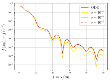
(a) Error vs Number of iterations

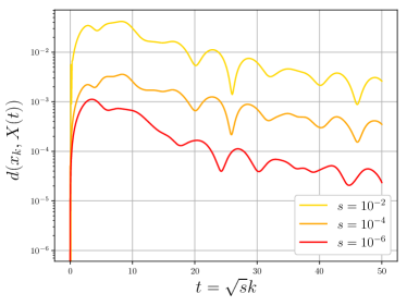
(b) Distance vs Number of iterations

Figure 4: Convergence of RNAG-C to the solution of ODE (6.1).

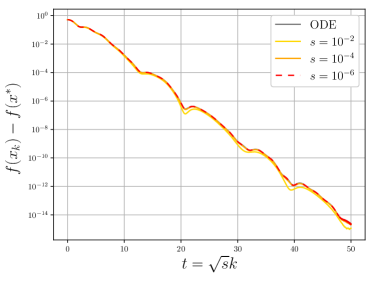
(a) Error vs Number of iterations

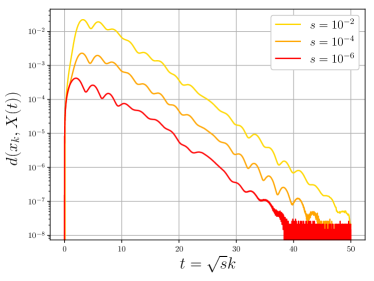
(b) Distance vs Number of iterations

Figure 5: Convergence of RNAG-SC to the solution of ODE (6.2).

Appendix H Proofs for Section 7

See 2

Proof.

For $x\in\mathbb{S}^{d-1}\subseteq\mathbb{R}^{d}$ and a unit tangent vector $v\in T_{x}M$, we have

$$\exp_{x}(tv)=\frac{x+\tan(t)\,v}{\left\|x+\tan(t)\,v\right\|}=\frac{x+\tan(t)\,v}{\sec(t)}$$

for $t\in I$, where $I$ is a small interval containing $0$. We consider the function $h:I\rightarrow M$ defined as

$$h(t) =f\left(\exp_{x}(tv)\right)$$

$$=-\frac{1}{2}\cos^{2}(t)\left(x+\tan(t)\,v\right)^{\top}A\left(x+\tan(t)\,v\right)$$

$$=-\frac{1}{2}h_{1}(t)h_{2}(t),$$

where $h_{1}(t)=\cos^{2}(t)$ and $h_{2}(t)=\left(x+\tan(t)\,v\right)^{\top}A\left(x+\tan(t)\,v\right)$. Note that $h_{1}(0)=1$, $h_{1}^{\prime}(0)=0$, $h_{1}^{\prime\prime}(0)=-2$, $h_{2}(0)=x^{\top}Ax$, $h_{2}^{\prime}(0)=2v^{\top}Ax$, and $h_{2}^{\prime\prime}(0)=2v^{\top}Av$. Now, by the product rule, we have

$$h^{\prime\prime}(0)=-\frac{1}{2}h_{1}^{\prime\prime}(0)h_{2}(0)-h_{1}^{\prime}(0)h_{2}^{\prime}(0)-\frac{1}{2}h_{1}(0)h_{2}^{\prime\prime}(0)=x^{\top}Ax-v^{\top}Av.$$

Because Rayleigh quotient is always in $\left[\lambda_{\min},\lambda_{\max}\right]$, we have $|h^{\prime\prime}(0)|\leq\left(\lambda_{\max}-\lambda_{\min}\right)$. This shows that $f$ is geodesically $\left(\lambda_{\max}-\lambda_{\min}\right)$-smooth. ∎

See 3

Proof.

When $K_{\max}\leq 0$, we have $\delta=1$. Let $\gamma:I\rightarrow M$ be a geodesic whose image is in $N$. It follows from Proposition 10 that

$$\frac{d^{2}}{dt^{2}}\frac{1}{2}d\left(\gamma(t),p_{i}\right)^{2} =\frac{d}{dt}\left\langle\log_{\gamma(t)}\left(p_{i}\right),-\gamma^{\prime}(t)\right\rangle$$

$$=\left\langle D_{t}\log_{\gamma(t)}\left(p_{i}\right),-\gamma^{\prime}(t)\right\rangle+\left\langle\log_{\gamma(t)}\left(p_{i}\right),-\gamma^{\prime\prime}(t)\right\rangle.$$

Note that $\gamma^{\prime\prime}(t)=0$ because $\gamma$ is a geodesic. Now, Proposition 1 gives $\frac{d^{2}}{dt^{2}}\frac{1}{2}d\left(\gamma(t),p_{i}\right)^{2}\geq 1$. ∎

References

- [1] F. Alimisis, A. Orvieto, G. Becigneul, and A. Lucchi, “A continuous-time perspective for modeling acceleration in riemannian optimization,” in Proceedings of the Twenty Third International Conference on Artificial Intelligence and Statistics, 2020, pp. 1297–1307.
- [2] N. K. Vishnoi, “Geodesic convex optimization: Differentiation on manifolds, geodesics, and convexity,” arXiv preprint arXiv:1806.06373, 2018.
- [3] A. Wiesel, “Geodesic convexity and covariance estimation,” IEEE transactions on signal processing, vol. 60, no. 12, pp. 6182–6189, 2012.
- [4] R. Hosseini and S. Sra, “Matrix manifold optimization for gaussian mixtures,” in Advances in Neural Information Processing Systems, 2015, pp. 910–918.
- [5] ——, “An alternative to em for gaussian mixture models: batch and stochastic riemannian optimization,” Mathematical Programming, vol. 181, no. 1, pp. 187–223, 2020.
- [6] S. Sra, “On the matrix square root via geometric optimization,” arXiv preprint arXiv:1507.08366, 2015.
- [7] P. Zadeh, R. Hosseini, and S. Sra, “Geometric mean metric learning,” in International Conference on Machine Learning, 2016, pp. 2464–2471.
- [8] V. A. Nguyen, S. Shafieezadeh-Abadeh, M.-C. Yue, D. Kuhn, and W. Wiesemann, “Calculating optimistic likelihoods using (geodesically) convex optimization,” arXiv preprint arXiv:1910.07817, 2019.
- [9] H. Zhang and S. Sra, “First-order methods for geodesically convex optimization,” in Conference on Learning Theory, 2016, pp. 1617–1638.
- [10] Y. E. Nesterov, “A method for solving the convex programming problem with convergence rate ,” in Dokl. akad. nauk Sssr, vol. 269, 1983, pp. 543–547.
- [11] P. Tseng, “On accelerated proximal gradient methods for convex-concave optimization,” submitted to SIAM Journal on Optimization, vol. 2, no. 3, 2008.
- [12] Y. Nesterov, Lectures on Convex Optimization. Springer, 2018, vol. 137.
- [13] C. Criscitiello and N. Boumal, “Negative curvature obstructs acceleration for geodesically convex optimization, even with exact first-order oracles,” arXiv preprint arXiv:2111.13263, 2021.
- [14] L. Hamilton and A. Moitra, “No-go theorem for acceleration in the hyperbolic plane,” arXiv preprint arXiv:2101.05657, 2021.
- [15] W. Su, S. Boyd, and E. Candes, “A differential equation for modeling nesterov’s accelerated gradient method: Theory and insights,” in Advances in Neural Information Processing Systems, 2014, pp. 2510–2518.
- [16] H. Zhang and S. Sra, “An estimate sequence for geodesically convex optimization,” in Proceedings of the 31st Conference On Learning Theory, 2018, pp. 1703–1723.
- [17] Y. Liu, F. Shang, J. Cheng, H. Cheng, and L. Jiao, “Accelerated first-order methods for geodesically convex optimization on riemannian manifolds,” in Advances in Neural Information Processing Systems, 2017, pp. 4868–4877.
- [18] F. Alimisis, A. Orvieto, G. Becigneul, and A. Lucchi, “Momentum improves optimization on riemannian manifolds,” in Proceedings of The 24th International Conference on Artificial Intelligence and Statistics, 2021, pp. 1351–1359.
- [19] K. Ahn and S. Sra, “From nesterov’s estimate sequence to riemannian acceleration,” in Proceedings of Thirty Third Conference on Learning Theory, 2020, pp. 84–118.
- [20] D. Martínez-Rubio, “Global riemannian acceleration in hyperbolic and spherical spaces,” arXiv preprint arXiv:2012.03618, 2021.
- [21] C. Criscitiello and N. Boumal, “An accelerated first-order method for non-convex optimization on manifolds,” arXiv preprint arXiv:2008.02252, 2020.
- [22] M. Lezcano-Casado, “Adaptive and momentum methods on manifolds through trivializations,” arXiv preprint arXiv:2010.04617, 2020.
- [23] M. Lezcano Casado, “Trivializations for gradient-based optimization on manifolds,” in Advances in Neural Information Processing Systems, 2019, pp. 9157–9168.
- [24] A. Wibisono, A. C. Wilson, and M. I. Jordan, “A variational perspective on accelerated methods in optimization,” proceedings of the National Academy of Sciences, vol. 113, no. 47, pp. E7351–E7358, 2016.
- [25] A. C. Wilson, B. Recht, and M. I. Jordan, “A lyapunov analysis of accelerated methods in optimization,” Journal of Machine Learning Research, vol. 22, no. 113, pp. 1–34, 2021.
- [26] V. Duruisseaux and M. Leok, “A variational formulation of accelerated optimization on riemannian manifolds,” arXiv preprint arXiv:2101.06552, 2021.
- [27] ——, “Accelerated optimization on riemannian manifolds via discrete constrained variational integrators,” arXiv preprint arXiv:2104.07176, 2021.
- [28] G. França, A. Barp, M. Girolami, and M. I. Jordan, “Optimization on manifolds: A symplectic approach,” arXiv preprint arXiv:2107.11231, 2021.
- [29] V. Duruisseaux and M. Leok, “Accelerated optimization on riemannian manifolds via projected variational integrators,” arXiv preprint arXiv:2201.02904, 2022.
- [30] J. M. Lee, Introduction to Riemannian manifolds. Springer, 2018, vol. 176.
- [31] P. Petersen, Riemannian Geometry, 3rd ed., ser. 171. Springer, Cham, 2016, vol. 1.
- [32] N. Boumal, “An introduction to optimization on smooth manifolds,” Available online, Aug 2020. [Online]. Available: http://www.nicolasboumal.net/book
- [33] J. Townsend, N. Koep, and S. Weichwald, “Pymanopt: A python toolbox for optimization on manifolds using automatic differentiation,” The Journal of Machine Learning Research, vol. 17, no. 1, pp. 4755–4759, 2016.
- [34] A. d’Aspremont, D. Scieur, and A. Taylor, “Acceleration methods,” arXiv preprint arXiv:2101.09545, 2021.
- [35] N. Miolane, N. Guigui, A. L. Brigant, J. Mathe, B. Hou, Y. Thanwerdas, S. Heyder, O. Peltre, N. Koep, H. Zaatiti, H. Hajri, Y. Cabanes, T. Gerald, P. Chauchat, C. Shewmake, D. Brooks, B. Kainz, C. Donnat, S. Holmes, and X. Pennec, “Geomstats: A python package for riemannian geometry in machine learning,” Journal of Machine Learning Research, vol. 21, no. 223, pp. 1–9, 2020.
- [36] H. Karcher, “Riemannian center of mass and mollifier smoothing,” Communications on pure and applied mathematics, vol. 30, no. 5, pp. 509–541, 1977.
- [37] D. A. Bini and B. Iannazzo, “Computing the karcher mean of symmetric positive definite matrices,” Linear Algebra and its Applications, vol. 438, no. 4, pp. 1700–1710, 2013.