First-order integer-valued autoregressive processes with Generalized Katz innovations

Abstract. A new integer-valued autoregressive process (INAR) with Generalised Lagrangian Katz (GLK) innovations is defined. We show that our GLK-INAR process is stationary, discrete semi-self-decomposable, infinite divisible, and provides a flexible modeling framework for count data allowing for under- and over-dispersion, asymmetry, and excess of kurtosis. A Bayesian inference framework and an efficient posterior approximation procedure based on Markov Chain Monte Carlo are provided. The proposed model family is applied to a Google Trend dataset which proxies the public concern about climate change around the world. The empirical results provide new evidence of heterogeneity across countries and keywords in the persistence, uncertainty, and long-run public awareness level.

Keywords: Bayesian inference, Big data, Counts time series, Climate Risk, Generalized Lagrangian Katz distribution, MCMC.

1 Introduction

In the recent years there has been a large interest in discrete-time integer-valued models, also due to increased availability of count data in very diverse fields including finance (Liesenfeld et al.,, 2006; Rydberg and Shephard,, 2003; Aknouche et al.,, 2021), economics (Freeland,, 1998; Freeland and McCabe,, 2004; Berry and West,, 2020), social sciences (Pedeli and Karlis,, 2011), sports (Shahtahmassebi and Moyeed,, 2016), image processing (Afrifa-Yamoah and Mueller,, 2022) and oceanography (Cunha et al.,, 2018). Among the modelling approaches, integer-valued autoregressive processes (INAR), introduced independently by Al-Osh and Alzaid, (1987) and McKenzie, (1985), become vary popular. The stochastic construction of the INAR relies on the binomial thinning operator and the properties of the model on the discrete self-decomposability of the stationary distribution of the process (Steutel and van Harn,, 1979). See also Weiß, (2008) and Scotto et al., (2015) for a review on thinning operators.

The original INAR model has been studied further in Al-Osh and Alzaid, (1987) and has been extend along different directions. (McKenzie,, 1986) introduced an INAR model with negative-binomial and geometric marginal distributions, Jin-Guan and Yuan, (1991) extended the INAR(1) model of Al-Osh and Alzaid, (1987) to the higher order INAR$(p)$. Al-Osh and Aly, (1992) introduced a negative-binomial INAR with a new iterated thinning operator. Other extensions of the INAR process has been made in order to include a seasonal structure in the model (e.g., see Bourguignon et al.,, 2016). INAR models with valued in the set of signed integers have been propose firstly by Kim and Park, (2008) and generalised by Alzaid and Omair, (2014) and Andersson and Karlis, (2014). Freeland, (2010) proposed a true integer-valued autoregressive model (TINAR(1)). More flexible INAR models have been introduced by assuming more flexible distributions for the innovations terms. Alzaid and Al-Osh, (1993) propose integer-valued ARMA process with Generalized Poisson marginals and Kim and Lee, (2017) introduced INAR with Katz innovations.

In this paper we extend further the Negative Binomial, Generalized Poisson and Katz INAR processes by assuming a more general distribution for the innovations which includes some well-known distributions used in time series of count data and some distributions which have not yet been used in modelling time series of counts. The two-parameter Katz distribution belongs to the Lagrangian Katz family together with the three-parameter Lagrangian Katz (e.g., see Consul and Famoye,, 2006, ch. 12). The Lagrangian Katz is a flexible distribution and naturally arises as first crossing probabilities, which is a common problem in actuarial mathematics, e.g. claim number distribution in cascading processes or ruin probability in discrete-time risk models. The Lagrangian Katz distribution has been extended further by Janardan, (1998) and Janardan, (1999) which introduced the four-parameter generalized Pólya-Eggenberger (GPED) distributions of the first and second kind. Janardan, (1998) showed that both families contain the Lagrangian Katz distribution as a special case. See also Johnson et al., (2005), ch. 2,5 and 7, for a review on the relationships between Lagrangian Katz distributions and other discrete distribution families. In this paper we consider the four-parameter GPED of the first kind, or Generalized Lagrangian Katz (GLK) distribution in the following, since it enjoys the properties of the Lagrangian distributions and includes some well-known distributions such as Generalized Poisson and Negative Binomial as special cases.

Another contribution of this paper regards the inference method. Various approaches to inference have traditionally presented for count data models, such as conditional likelihood approach, generalized method of moments and Yule-Walker approach. See Weiß and Kim, (2013) for a review. Despite the popularity gained in the recent years by Bayesian methods, the applications to count data models are still limited (e.g., see McCabe and Martin,, 2005; Neal and Subba Rao,, 2007; Drovandi et al.,, 2016; Shang and Zhang,, 2018; Garay et al., 2020b, ). Thus, we provide a Bayesian inference procedure for our model and illustrate the efficiency of the procedure on a synthetic dataset. The Bayesian approach to inference entirely considers parameter uncertainty in the prior knowledge about a random process and allows for imposing parameter restrictions through the specification of the prior distribution (Chen and Lee,, 2016). The posterior distribution of the parameters quantifies uncertainty in the estimation (Chen and Lee,, 2017), which can be included in the prediction. The inference from the Bayesian perspective may result in richer inferences in the case of small samples (Garay et al., 2020a, ) and extra-sample information and in robust inference in the presence of outliers (Fried et al.,, 2015). Finally, model selection for both nested and non-nested models can be easily carried out.

We illustrate the model’s flexibility with an application to an original Google Trend dataset on measures of public concern about climate change in different countries. Assessing the level of public awareness and knowledge in a specific topic and understanding the dynamics in the social consciousness allows for designing more effective public policies. For this reason, researchers measured and studied the level of awareness about the effects of climate change in different sectors of society such as households (Frondel et al.,, 2017), winegrowers (Battaglini et al.,, 2009), farmers (Fahad and Wang,, 2018; Singh et al.,, 2017), mountain peoples (Ullah et al.,, 2018). Most of these studies rely on surveys conducted in a specific geographical area and sector of society, with a few exceptions. For example, Ziegler, (2017) proposed a cross-country analysis of climate change beliefs and attitudes. Lineman et al., (2015) provided a broader and global perspective by exploiting the potentiality of big data provided by Google Trend. This extended climate change perception literature along two lines. First, we consider a multi-country dataset including country-specific measures to capture heterogeneity across the world in public awareness. Moreover, we offer a model-based approach and an inference procedure to analyze these measures, which allow for a better comprehension of the cross-country and cross-keyword heterogeneity in the long-run level of public perception and perception uncertainty and persistence.

The paper is organized as follows. Section 2 introduces the Generalized Lagrangian Katz family, the INAR process, and some of their properties. Section 3 proposes a Bayesian inference procedure and provides some simulation results. Section 4 illustrates the model and inference framework on a multi-country Google Trend dataset on climate change and provides some new findings in the public interest in climate change. Section 5 concludes.

2 INAR(1) with generalized Katz innovations

2.1 Generalized Lagrangian Katz family

The Generalized Lagrangian Katz (GLK) distribution has been introduced by (Janardan,, 1998), which named the distribution Generalized Polya Eggenberger distribution. (Consul and Famoye,, 2006) argued that since the distribution it is not related to the Polya, it should be name Generalized Lagrangian Katz distribution. The GLK has probability mass function (pmf), $P(X=x)=p_{x}$, defined as

$$p_{x}=\frac{1}{x!}\beta^{x}\frac{a}{c}\frac{1}{(\frac{a}{c}+x\frac{b}{c}+x)}(1-\beta)^{\frac{a}{c}+x\frac{b}{c}}\left(\frac{a}{c}+x\frac{b}{c}+1\right)_{{x}\uparrow}\,\,x=0,1,2,\ldots\ \\$$ (1)

where $(x)_{{k}\uparrow}=x(x+1)\ldots(x+k-1)$ is the rising factorial with the convention that $(x)_{0}=1$, and $a>0$, $c>0$, $b\geq 0$ and $0<\beta<1$ are the parameters. In the following, we denote the distribution with $\mathcal{GLK}(a,b,c,\beta)$.

The GLK distribution has generating function (pgf)

$$H(u)=\sum_{x=0}^{\infty}p_{x}u^{x}$$ (2)

which satisfies:

$$H(u)=(1-\beta+\beta z)^{a/c},\,\,z=u(1-\beta+\beta z)^{b/c+1},$$ (3)

or alternatively

$$H(u)=\left(\frac{1-\beta}{1-\beta z}\right)^{a/c},\,\,z=u\left(\frac{1-\beta z}{1-\beta}\right)^{b/c},$$ (4)

see Janardan, (1998).

Remark 1 (Parameter space).

The definition of GLK given in Janardan, (1998) is obtained as a special case of ”generalized Lagrangian distribution” starting from the Lagrangian expansion

$$H(u)=f(0)+\sum_{x=1}^{\infty}\frac{u^{x}}{x!}\left|\partial^{x-1}(g^{x}(z)f^{\prime}(z))\right|_{z=0}$$

where $H(u)=f(z)$ for $u$ satisfying $z=ug(z)$, (Consul and Famoye,, 2006, p. 10-11). Choosing $g(z)=((1-\beta)/(1-\beta z))^{b/\beta}$ and $f(z)=((1-\beta)/(1-\beta z))^{a/c}$, one gets (3) and (1) follows after some algebra. See Appendix A for details. While with this construction $\sum_{x\geq 0}p_{x}=1$ is granted by the condition $H(1)=f(1)=1$, some constrains on the parameters are needed in order to have all the $p_{x}:=\frac{1}{x!}\partial^{x-1}(g^{x}(z)f^{\prime}(x))|_{x=0}>0$. Three different cases are discussed below.

• For parameter values $a>0,b\geq 0,c>0$ the pmf are positive. Moreover, for $a/c,b/c\in\mathbb{N}$ the extended binomial coefficient $((a+bx)/c+1)_{x\uparrow}/x!$ coincides with the standard binomial coefficient ${\frac{a+bx}{c}+x\choose x}$ (Consul and Famoye,, 2006, p. 8).

• For $-c<b<0$, $a/c,b/c\in\mathbb{N}$ and $(c-a)/(c+b)\leq(a+c)/|b|$, the pmf are positive for $x<x^{*}=(a+c)/|b|$, while $p_{x}=0$ for $x\geq x^{*}$.

• If $-c<b<0$ but the additional constraints of the previous point are not satisfied, the terms appearing in the product $({(a+bx)}/{c}+1)_{x\uparrow}$ change sing and there is no guarantee that the result is positive. Indeed, for all the $x$ such that $x>\max\{(a+1)/|b|,(c-a)/(c+b),2\}$ one has $(a+bx)/c+1<0$ and $(a+bx)/c+x-1>0$ and hence there is an integer $q=q_{x}$ such that $(a+bx)/c+m<0$ for $1\leq m\leq q$ and $(a+bx)/c+m>0$ for $q+1\leq m\leq k-1$. Hence

  $$\frac{1}{\frac{a+bx}{c}+x}\Big{(}\frac{(a+bx)}{c}+1\Big{)}_{x\uparrow}=(-1)^{q}\prod_{m=1}^{q}\Big{|}\frac{(a+bx)}{c}+m\Big{|}\prod_{m=q+1}^{k-1}\Big{|}\frac{(a+bx)}{c}+m\Big{|}$$

  which is negative whenever $q_{x}$ is odd. For example take $a=10$, $b=-1$ and $c=2$, for $x=20$ one has $q_{20}=5$, which shows that $p_{20}<0$ which clearly is impossible.

It should be noted that alternative definitions for $-c<b<0$ can be considered. For example one can set to 0 the $p_{x}<0$, i.e. when $x>\max\{(a+1)/|b|$. In this case re-scaling the $p_{x}$ is necessary to get $\sum_{x=0}^{x^{*}}p_{x}=1$. The resulting pmf is no more a generalized Lagrangian distribution (due to the truncation and rescaling) and the normalizing constant is not in closed form. See for example McCabe and Skeels, (2020) for a discussion on the parameter values for the Katz distributions. In this paper we restrict our attention on the family of GLK and rule out negative pmf values by assuming $b\geq 0$. Our modelling and inference framework can be easily extend to account for these distributions.

The following remarks clarify the relationship with other definitions of Katz distributions and with other discrete distributions. For some values of the parameters, the GLK distribution reduces either to some well known distributions in time series analysis, or to distributions which have not yet been used in count data modelling.

Remark 2.

Three distributions related to our research are: (i) the Lagrangian Katz distribution $\mathcal{LK}(a,b,\beta)$ by replacing $c$ with $\beta$, (which is called Generalized Katz in (Consul and Famoye,, 2006)); (ii) the Katz distribution $\mathcal{K}(a,\beta)$ for $b=0$ and by replacing $c$ with $\beta$ (Katz,, 1965); (iii) the Polya-Eggenberger distribution $\mathcal{PE}(a,c,\beta)$ for $b=0$ (Janardan,, 1998). Note that the Katz distribution in Consul and Famoye, (2006), Tab. 2.1, is not the Katz distribution of Katz, (1965), it corresponds instead to the Generalized Polya Eggenberger of the first type (GPED₁-I) of Janardan, (1998) and can be obtain as the limit of the zero-truncated GLK for $a\rightarrow-c$.

The probability mass function of the GLK for different parameter settings given in Fig. 1. In the top-left plot we compare $\mathcal{LK}(a,c)$, $\mathcal{LK}(a,b,\beta)$ and $\mathcal{GLK}(a,b,c,\beta)$ with the same mean. The top-right plot illustrates the sensitivity of the $\mathcal{GLK}(a,b,c,\beta)$ pmf with respect to the different parameters. All distributions have the same mean (vertical dashed line). The bottom plots illustrate the effects of the parameters on the tails (log-scale) for a $\mathcal{GLK}(a,b,c,\beta)$ with over-dispersion $VMR=50/15$ (left) and under-dispersion $VMR=13/15$ (right).

Remark 3.

The following standard distributions have been used to define INAR processes: (i) the Negative Binomial distribution $\mathcal{NB}(r,p)$ for $b=0$ $\beta=1-p$ and $r=a/c$; (ii) the Binomial distribution $\mathcal{B}in(n,p)$ for $c=1$, $b=-1$, $a=n\in\mathbb{N}$ and $\beta=p$; the Poisson distribution $\mathcal{P}(\theta)$ for $c\rightarrow 0$, $b\rightarrow 0$ s.t. $a\beta/c=\theta$.

Remark 4.

The GLK family includes also the generalizations of the distributions given in the previous remark, that are the Generalized Negative Binomial distribution $\mathcal{GNB}(r,\gamma,p)$ for $c=1$, $a=r$, $b=\gamma-1$ and $\beta=p$ and the Generalized Poisson (GP) distribution $\mathcal{GP}(\theta,\lambda)$ for $c\rightarrow 0$ s.t. $\frac{b}{a}=\lambda$ and $a\beta/c=\theta>0$ with $0<\lambda<\theta^{-1}$. The GP limit of the GLK distribution is stated in (Consul and Famoye,, 2006) without proof. In Appendix A we provide a proof of the result.

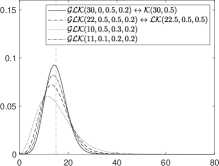
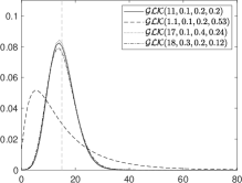
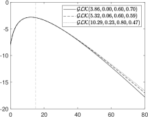
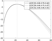
Figure 1: Probability mass function of the Generalized Lagrangian Katz for different parameter settings. Top left: comparison between $\mathcal{LK}(a,c)$, $\mathcal{LK}(a,b,\beta)$ and $\mathcal{GLK}(a,b,c,\beta)$. Top right: sensitivity of $\mathcal{GLK}(a,b,c,\beta)$ with respect to the parameters. Bottom: effect of the parameters on the tails (log scale) for a $\mathcal{GLK}(a,b,c,\beta)$ with over-dispersion ($VMR=50/15$, left) and under-dispersion ($VMR=13/15$, right). In each plot the distribution mean (vertical dashed line).

Studying the moments allows for a better understanding of the flexibility of the GLK distribution. Four moments relevant to our analysis are the following.

Proposition 1.

Let $X\sim\mathcal{GLK}(a,b,c,\beta)$, define $\mu_{k}^{\prime}=\mathbb{E}((X-\mathbb{E}(X))^{k})$ and $\mu_{k}=\mathbb{E}(X^{k})$ then

$$\mu_{1} = \frac{a\theta}{\kappa},\quad\quad\mu_{2}^{\prime}=\frac{(1-\beta)a\theta}{\kappa^{3}},\quad\quad\mu_{3}^{\prime}=\frac{a\theta(1-2\beta)(1-\beta)}{\kappa^{4}}+\frac{3a\theta^{2}(1-\beta)^{2}(b+c)}{\kappa^{5}}$$

$$\mu_{4}^{\prime} = a\theta(1-\beta)(1+2\theta b-(b+c)\beta\theta)\left(\frac{1-\beta-\beta^{2}}{\kappa^{6}}+\frac{5a\theta(1-\beta)(b+c)}{\kappa^{7}}\right)+3(\mu_{2}^{\prime})^{2}$$

where $\kappa=1-\beta-b\beta/c$ and $\theta=\beta/c$.

For a proof, see Janardan, (1998) Theorems 1-3. Another quantity of interest is the coefficient of variation which represents a measure of relative dispersion, given by the standard deviation to mean ratio. From the previous result it follows that the coefficient of variation is

$$CV=\left(\frac{(1-\beta)}{a\theta\kappa}\right)^{1/2}.$$

Another classical measure of dispersion is the Fisher index, given by the variance-to-mean ratio

$$VMR=\frac{(1-\beta)}{\kappa^{2}},$$

which does not depend on the parameter $a$. For a given $\beta$, following the values of $\kappa$ ($b$ and $c$), the distribution allows for various degree of dispersion: not dispersed ($VMR=0$), under-dispersed ($VMR<1$), equally dispersed ($VMR=1$) and over-dispersed ($VMR>1$).

(a) Mean ($\mu_{1}$)	(b) Index of Dispersion ($VMR$)
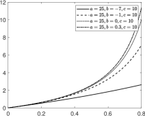
(c) Skewness ($S$)	(d) Kurtosis ($K$)

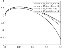
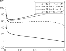
Figure 2: GLK moments when increasing the value of $\beta$ (horizontal axis) for different values of $b$ (lines).

The skewness and the kurtosis of the distribution are

$$S = \frac{(1-2\beta)\kappa^{1/2}}{((1-\beta)a\theta)^{1/2}}+\frac{3((1-\beta)\theta)^{1/2}(b+c)}{a\kappa^{1/2}},$$ (5)

$$K = (1+2b\theta-(b+c)c\theta^{2})\left(\frac{(1-\beta-\beta^{2})}{a\theta(1-\beta)}+\frac{5(b+c)}{\kappa}\right)+3,$$ (6)

respectively. For a given value of $\theta$, there is negative skewness if $\beta<(1+\xi)/(2\kappa+\xi)$ with $\xi=3\theta(b+c)a^{-1/2}$ and positive otherwise.

Figure 2 illustrates the effect of the parameter values on the mean, index of dispersion, skewness and kurtosis. Increasing the value of $\beta$ (horizontal axis) the $\mathcal{GLK}(a,b,c,\beta)$ distribution allows for different types of dispersion (panel b), for both negative and positive skewness (panel c) and for various degrees of excess of kurtosis (panel d).

We conclude this section with an important property of the GLK distribution.

Proposition 2.

A random variable $X\sim\mathcal{GLK}(a,b,c,\beta)$ is infinite divisible, in particular $X\stackrel{{\scriptstyle\mathcal{L}}}{{=}}\sum_{j=1}^{n}X_{jn}$ where $X_{jn}\stackrel{{\scriptstyle iid}}{{\sim}}\mathcal{GLK}(a/n,b,c,\beta)$.

See Appendix for a proof based on the properties of the pgf function.

2.2 A INAR(1) process

The Generalized Katz INAR(1) process (GLK-INAR(1)) is defined by means of the binomial thinning operator, $\circ$. The binomial thinning for a non-negative discrete random variable $X$ is defined as

$$\alpha\circ X=\sum_{i=1}^{X}B_{i}(\alpha)$$ (7)

where $B_{i}(\alpha)$ are iid Bernoulli r.v.s with success probability $P(B_{i}(\alpha)=1)=\alpha$.

Definition 1 (GLK-INAR process).

For $\alpha\in(0,1)$, the GLK-INAR(1) process is defined by

$$X_{t}=\alpha\circ X_{t-1}+\varepsilon_{t},\qquad t\in\mathbb{Z}$$ (8)

where $\varepsilon_{t}$ are iid random variables with Generalized Lagrangian Katz distribution $\mathcal{GLK}(a,b,c,\beta)$, independent of $X_{s}$, $s\leq t-1$.

Figure 3 provides some trajectories of $T=100$ points each, simulated from a GLK-INAR(1) with innovation distributions given by the solid lines in the bottom plots of Fig. 1, that are $\mathcal{GLK}(3.86,0,0.60,0.70)$ (overdispersion) and $\mathcal{GLK}(25.00,0.00,0.70,0.42)$ (underdispersion). The trajectories correspond to two parameter settings we find the empirical application to climate change discussed in Section 4, that are: (i) high persistence setting ($\alpha=0.7$, left); (ii) low persistence setting ($\alpha=0.3$, right). In all plots, the empirical mean of the observations is reported (dashed line) as a reference to illustrate the different level of persistence in the trajectories.

(a) Over-dispersed innovations
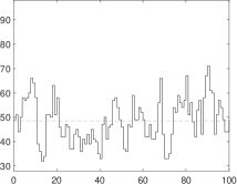
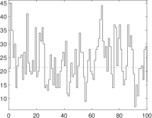
(a) Under-dispersed innovations

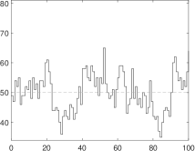
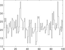
Figure 3: Trajectories of the GLK-INAR(1) in the high ($\alpha=0.7$, left column) and low persistence ($\alpha=0.3$, right column) regimes. The trajectories in the over- and under-dispersion settings are in the rows. In all plots, the empirical mean of the observations (dashed line).

Thanks to the general parametric family assumed, by setting $b=0$, $c=\beta=\theta_{1}$ and $a=\theta_{2}$, our GLK-INAR(1) nests the INARKF(1) of Kim and Lee, (2017) as special case. The GLK-INAR(1) naturally nests the Poisson INAR(1) of Al-Osh and Alzaid, (1987), the Negative Binomial INAR(1) of Al-Osh and Aly, (1992), and the Generalized Poisson INAR(1) of Alzaid and Al-Osh, (1993).

As any INAR process, the GLK-INAR(1) has the following representation

$$X_{t+k}=\alpha^{k}\circ X_{t}+\sum_{j=0}^{k-1}\alpha^{j}\circ\varepsilon_{t+1-j}$$ (9)

and its conditional pgf can be written as

$$H_{X_{t+k}|X_{t}}(u)=(1-\alpha^{k}+\alpha^{k}u)^{X_{t}}\prod_{j=0}^{k-1}H(1-\alpha^{j}+\alpha^{j}u)$$ (10)

where $H(u)$ is defined in Eq. 3 or in Eq. 4. Details are given in Appendix A. The previous representation allows us to derive the following properties, which are useful in forecasting.

Theorem 1.

The conditional mean and variance of the process GLK-INAR(1) $\{X_{t},t\in\mathbb{Z}\}$ are

$$\mathbb{E}(X_{t+k}|X_{t})=\alpha^{k}X_{t}+\frac{1-\alpha^{k-1}}{1-\alpha}\frac{a\theta}{\kappa}$$ (11)

$$\mathbb{V}(X_{t+k}|X_{t})=(\alpha^{k}-\alpha^{2k})X_{t}+\frac{1-\alpha^{2k}}{1-\alpha^{2}}\left(\frac{a(1-\beta)\theta}{\kappa^{3}}-\frac{a\theta}{\kappa}\right)+\frac{1-\alpha^{k}}{1-\alpha}\frac{a\theta}{\kappa}$$ (12)

where $\kappa=1-\beta-b\beta/c$ and $\theta=\beta/c$.

Remark 5.

Setting $b=0$, $c=\beta=\theta_{1}$ and $a=\theta_{2}$ the results in Kim and Lee, (2017) Th. 2.2 are obtained.

Remark 6.

Since $\alpha<1$, $\underset{k\rightarrow\infty}{\lim}\mathbb{E}(X_{t+k}|X_{t})=a\theta/(\kappa(1-\alpha)$ and $\underset{k\rightarrow\infty}{\lim}\mathbb{V}(X_{t+k}|X_{t})=a\theta((1-\beta)+\alpha\kappa^{2})/((1-\alpha^{2})\kappa^{3})$ where $\kappa=1-\beta-b\beta/c$ and $\theta=\beta/c$.

The process $\{X_{t}\}_{t\in\mathbb{Z}}$ is a Markov Chain on $\mathbb{N}$ and the transition probability $P_{i,j}=\mathbb{P}(X_{t}=j|X_{t-1}=i)$ can be expressed as

$$P_{i,j}=\sum_{k=0}^{\min(i,j)}\mathbb{P}(\alpha\circ X_{t-1}=k|X_{t-1}=i)\mathbb{P}(\varepsilon=j-k)$$

$$=\sum_{k=0}^{\min(i,j)}\binom{i}{k}\alpha^{k}(1-\alpha)^{i-k}p_{j-k}$$ (13)

where $p_{x}$ is the pmf given in Eq. 1.

Theorem 2.

The process $\{X_{t}\}_{t\in\mathbb{Z}}$ is an irreducible, aperiodic and positive recurrent Markov chain. Hence there is a unique stationary distribution for the process $\{X_{t}\}_{t\in\mathbb{Z}}$.

See Appendix A for a proof. The result extends to the case of GLK innovations, the stationarity for INAR(1) with power series innovations given in Bourguignon and Vasconcellos, (2015) and with Katz distribution given in Kim and Lee, (2017).

From Th. 2 it follows that there is a strong stationary process with stationary distribution $P_{j}$, $j\in\mathbb{N}$, given by the marginal distribution

$$P_{j}=\sum_{i=0}^{\infty}P_{i,j}P_{i}.$$ (14)

Since at stationarity the process satisfies $X=\alpha\circ X+\varepsilon$, where $\varepsilon\sim\mathcal{GLK}(a,b,c,\beta)$, and the innovation terms are infinite divisible by Theorem 2, the stationary distribution satisfies the following definition of discrete semi-self-decomposability given in Bouzar, (2008).

Definition 2.

A nondegenerate distribution $\{p_{x},\,x\in\mathbb{N}\}$ on $\mathbb{N}$ is said to be discrete semi-self-decomposable (DSSD) of order $\alpha\in(0,1)$ if its pgf $\Psi(z)$ satisfies for all $|z|\leq 1$

$$\Psi(z)=\Psi(1-\alpha-\alpha z)\Psi_{\alpha}(z)$$

where $\Psi_{\alpha}(z)$ is the pgf of an infinitely divisible distribution.

Being the stationary distribution a DSSD, Th. 2 in Bouzar, (2008) yields that it is also infinitely divisible.

Theorem 3.

The marginal distribution of the stationary process $\{X_{t}\}_{t\in\mathbb{Z}}$ is infinitely divisible.

Since the GLK distribution satisfies the convolution property (see Janardan,, 1998, Th. 8), then the GLK-INAR(1) is stable by aggregation as stated in the following

Theorem 4.

Let $\{X_{jt}\}_{t\in\mathbb{Z}}$ with $j=1,2,\ldots,J$ be a sequence of independent GLK-INAR(1) which satisfy:

$$X_{jt}=\alpha\circ X_{jt-1}+\varepsilon_{jt},\quad\varepsilon_{jt}\sim\mathcal{GLK}(a_{j},b,c,\beta)$$ (15)

The process $Y_{t}=X_{1t}+\ldots+X_{Jt}$ is GLK-INAR(1) which satisfies:

$$Y_{t}=\alpha\circ Y_{t-1}+\varepsilon_{t},\quad\varepsilon_{t}\sim\mathcal{GLK}(a_{1}+\ldots+a_{J},b,c,\beta)$$ (16)

Stationarity yields the following unconditional movements of the process.

Theorem 5.

Let $\mu_{\varepsilon}$, $\mu_{\varepsilon}^{(2)}$ and $\sigma^{2}_{\varepsilon}$ the mean, second order non-central moment and variance given in Prop. 1 for a $\mathcal{GLK}(a,b,c,\beta)$. For a GLK-INAR(1) process, the following unconditional moments can be derived:

1. $\mu_{X}=\mathbb{E}(X_{t})=\mu_{\varepsilon}/(1-\alpha)$

2. $\mu_{X}^{(2)}=\mathbb{E}(X_{t}^{2})=(\alpha\mu_{\varepsilon}+2\alpha\mu_{\varepsilon}^{2}/(1-\alpha)+\mu_{\varepsilon}^{(2)})/(1-\alpha^{2})$

3. $\mathbb{E}(X_{t}X_{t-k})=\alpha\mathbb{E}(X_{t-1}X_{t-k})+\mu_{\varepsilon}\mu_{X}$

4. Higher order non-central moments can be derived using the formula:

   $$\mu_{X}^{(m)}=\sum_{i=0}^{m}\sum_{k=0}^{i-1}\sum_{l=0}^{i-k}{i\choose k}(1-\alpha^{i})^{-1}S(m,i)s(i-k,l)\alpha^{k}\mu_{X}^{(\underline{k})}\mu_{\varepsilon}^{(l)}$$ (17)

   where $s(m,k)$ and $S(m,k)$ denote the Stirling’s numbers of the I and II kind, respectively.

From the previous theorem one obtains the unconditional variance of the process $\sigma^{2}_{X}=\mathbb{V}(X_{t})=(\sigma_{\varepsilon}^{2}+\alpha\mu_{\varepsilon})/(1-\alpha^{2})$ and the dispersion index of the process

$$VMR_{X}=\frac{\sigma^{2}_{X}}{\mu_{X}}=\frac{VMR_{\varepsilon}+\alpha}{1+\alpha}=\frac{1}{1+\alpha}\left(\alpha+\frac{1-\beta}{(1-\beta-b\beta/c)^{2}}\right)$$ (18)

where $VMR_{\varepsilon}=\sigma_{\varepsilon}^{2}/\mu_{\varepsilon}$ is the innovation index of dispersion. It follows that there is under- or over-dispersion in the marginal distribution, $VMR_{X}<1$ and $VMR_{X}>1$, if and only if there is under- or over-dispersion in the innovation, $VMR_{\varepsilon}<1$ or $VMR_{\varepsilon}<1$ respectively.

The autocorrelation function is

$$\gamma_{k}=\mathbb{C}ov(X_{t},X_{t-k})=\mathbb{E}(X_{t}X_{t-k})-\mu_{X}^{2}=\alpha^{k}\sigma^{2}_{X}$$ (19)

as in the INAR(1) process (e.g., see Al-Osh and Alzaid,, 1987).

3 Bayesian inference

3.1 Posterior distribution

Let us assume the following prior distributions

$$\alpha\sim\mathcal{B}e(\kappa_{\alpha},\tau_{\alpha}),\quad a\sim\mathcal{G}a(\kappa_{a},\tau_{a}),\quad b\sim\mathcal{G}a(\kappa_{b},\tau_{b}),$$ (20)

$$c\sim\mathcal{G}a(\kappa_{c},\tau_{c}),\quad\beta\sim\mathcal{B}e(\kappa_{\beta},\tau_{\beta})$$ (21)

where $\mathcal{B}e(\kappa,\tau)$ is the beta distribution with shape parameters $\kappa$ and $\tau$ and $\mathcal{G}a(\kappa,\tau)$ the gamma distribution with shape and scale parameters $\kappa$ and $\tau$, respectively. In the empirical applications we assume a non-informative hyper-parameter setting for $\alpha$ and $\beta$, that is $\kappa_{\alpha}=\tau_{\alpha}=\kappa_{\beta}=\tau_{\beta}=1$ and an informative prior for $a,b$ and $c$ with $\kappa_{a}=\tau_{a}=1$, $\kappa_{b}=\kappa_{c}=2$ and $\tau_{b}=\tau_{c}=1/2$.

Let $x_{1},\ldots,x_{T}$ be a sequence of observations for the GLK-INAR(1) process, then the joint posterior distribution is given by

$$\pi(\theta|x_{1},\ldots,x_{T})\propto\pi(\theta)\prod_{t=1}^{T}\prod_{i=0}^{\infty}\prod_{j=0}^{\infty}P_{ij}(\theta)^{\mathbb{I}(x_{t}-j)\mathbb{I}(x_{t-1}-i)}$$ (22)

where $\theta=(\alpha,a,b,c,\beta)$ is the parameter vector $\pi(\theta)$ the joint prior and

$$P_{ij}(\theta)=\sum_{k=0}^{\min(i,j)}\binom{i}{k}\alpha^{k}(1-\alpha)^{i-k}\frac{\frac{a}{c}}{\frac{a+bx}{c}+j-k}\binom{\frac{a+b(j-k)}{c}+j-k}{j-k}\beta^{j-k}(1-\beta)^{\frac{a+b(j-k)}{c}}.$$

Remark 7 (Parameters space).

Following the discussion in Remark 1, if the parameter constrain $c>0$ is not imposed the coefficients of the Lagrangian expansion can be negative. In this case a truncated GLK can be used, similarly to what is proposed in McCabe and Skeels, (2020) for the Katz distribution, and the inference procedure can be easily extended to include this type of distributions. The truncation can be imposed by using the following recursion for the transition probability:

$$p_{i}(\theta)=p_{0}\prod_{j=0}^{i-1}\max\left\{0,\frac{U(\theta)+V(\theta)j}{a+j}\right\}$$ (23)

where $U(\theta)=a\beta/c$, $V(\theta)=U(b+c)/(a+b)$ and

$$p_{0}=\left(1+\sum_{j=1}^{\infty}\prod_{k=0}^{j-1}\max\left\{0,\frac{U(\theta)+V(\theta)j}{a+j}\right\}\right)^{-1}.$$ (24)

The probability $p_{i}$ becomes null for $i>j$ if $U(\theta)+V(\theta)j<0$ at $j$.

Since the joint posterior is not tractable we follow a Markov Chain Monte Carlo (MCMC) framework to posterior approximation. See Robert and Casella, (2013) for an introduction to MCMC methods. We overcome the difficulties in tuning the parameters of the MCMC procedure by applying the Adaptive MCMC sampler (AMCMC) proposed in Andrieu and Thoms, (2008). Following a standard procedure, the following reparametrization is considered to impose the constrains to the parameters of the GLK-INAR(1). Let $\eta$ be the parameter vector of dimension $q$ obtained by the transformation $\varphi(\theta)$

$$\eta_{1}=\log(\eta_{1}/(1-\eta_{1})),\quad\eta_{2}=\log(\theta_{2})$$ (25)

$$\eta_{3}=\log(\theta_{3}),\quad\eta_{4}=\log(\theta_{4}),\quad\eta_{5}=\log(\eta_{5}/(1-\eta_{5}))$$ (26)

and let $\pi(\eta|x_{1},\ldots,x_{T})=\pi(\varphi^{-1}(\eta)|x_{1},\ldots,x_{T})J(\eta)$ be the posterior of $\eta$, with $J(\eta)=\theta_{1}\theta_{2}\theta_{3}\theta_{4}\theta_{5}(1-\theta_{1})(1-\theta_{5})$ the Jacobian of the transformation $\varphi$ given above. Given the adaptation parameters $\mu^{j}$ and $\Sigma^{(j)}$, at the $j$-th iterations, the AMCMC consists of the following three steps. First, a candidate $\eta^{\ast}$ is generated from the following proposal distribution

$$\eta^{\ast}=\eta^{(j-1)}+\lambda^{(j)}w^{(j)},\quad w^{(j)}\sim\mathcal{N}_{q}(\mathbf{0},\Sigma^{(j)}).$$ (27)

Second, the candidate is accepted with probability $\rho^{(j)}=\rho(\eta^{(j-1)},\eta^{\ast})$, and third, the adaptive parameters are updated as follows:

$$\mu^{(j+1)} = \mu^{(j)}+\gamma^{(j)}(\mu^{(j)}-\eta^{(j)})$$ (28)

$$\Sigma^{(j+1)} = \Sigma^{(j)}+\gamma^{(j)}((\mu^{(j)}-\eta^{(j)})(\mu^{(j)}-\eta^{(j)})^{\prime}-\Sigma^{(j)})$$ (29)

$$\log\lambda^{(j+1)} = \log\lambda^{(j)}+\gamma^{(j)}(\rho^{(j)}-\rho^{\ast})$$ (30)

where $\rho^{*}=0.4$ is the target acceptance probability and $\gamma^{(j)}=j^{-1.6}$ is the adaptive scale (Andrieu and Thoms,, 2008, , Algorithm 4).

3.2 Simulation results

We illustrate the effectiveness of the Bayesian procedure in recovering the true value of the parameters and the efficiency of the MCMC procedure through some simulation experiments. We test the efficiency of the algorithm in two different settings, which can be commonly found in the data: low persistence and high persistence (see trajectories in Fig. 3). The true values of the parameters are: $\alpha=0.3$, $a=5.3239$,$b=0.0592$, $c=0.6$, $\beta=0.5917$ in the low persistence setting, and $\alpha=0.7$, $a=5.3239$,$b=0.0592$, $c=0.6$, $\beta=0.5917$ in the high persistence setting. For each setting we run the Gibbs sampler for 50,000 iterations on each dataset, discard the first 10,000 draws to remove dependence on initial conditions, and finally apply a thinning procedure with a factor of 10, to reduce the dependence between consecutive draws.

High-persistence setting
$\alpha$	$a$
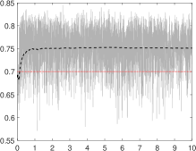
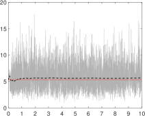
$b$	$c$
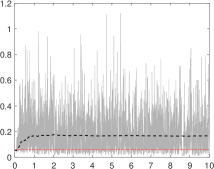
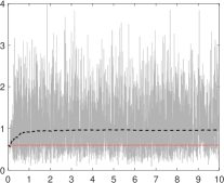
$\beta$	$a\beta/(c-c\beta-\beta b)$

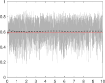
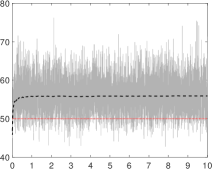
Figure 10: MCMC output for the parameters of the GLK-INAR(1). In all plots, the MCMC draws (gray solid), the progressive MCMC average (dashed black) over the iterations (horizontal axis in thousands), and the true value of the parameter (horizontal red dashed).

For illustrative purposes, we show in Figures 4 the MCMC posterior approximation for the parameter $\alpha$ (first row), the unconditional mean of the process (second row), and the marginal likelihood (last row), in one of our experiments for the high- and low-persistence settings. In each plot the true value (solid black line) and the Bayesian estimates approximated by using 4,000 MCMC samples after thinning and burn-in removal (dashed red line). For illustrative purposes, Fig. 10-11 and 12-13 in Appendix B exhibit 10,000 MCMC posterior draws and the MCMC approximation of the posterior distribution for all the parameters, in the high- and low-persistence settings.

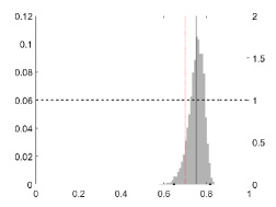
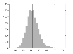
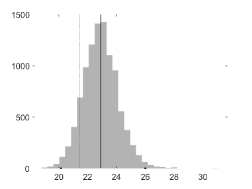
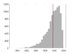
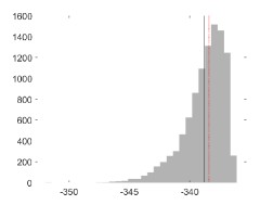
Figure 4: MCMC approximation of the posterior distribution (histogram) of the parameters $\alpha$ (top), the unconditional mean $\mu_{\varepsilon}/(1-\alpha)$ (middle) and the marginal likelihood (bottom) of the GLK-INAR(1) in the high-persistence (left) and low-persistence (right) setting. In all plots, the true parameter value (red dashed) and the estimated one (black solid).

In our experiments the acceptance rate is in the range of 40%-53% for both parameter settings. Table 1 shows, for all the parameters the autocorrelation function (ACF), effective sample size (ESS), inefficiency factor (INEFF) and Geweke’s convergence diagnostic (CD) before (BT subscript) and after thinning (AT subscript). The numerical standard errors are evaluated using the nse package (Geyer,, 1992; Ardia and Bluteau,, 2017; Ardia et al.,, 2018).

	Low persistence					High persistence
	$\alpha=0.3$, $a=5.3239$, $b=0.0592$, $c=0.6$, $\beta=0.5917$					$\alpha=0.7$, $a=5.3239$, $b=0.0592$, $c=0.6$, $\beta=0.5917$
	$\alpha$	$a$	$b$	$c$	$\beta$	$\alpha$	$a$	$b$	$c$	$\beta$
$ACF(1)_{BT}$	0.93	0.92	0.93	0.92	0.94	0.94	0.92	0.93	0.92	0.94
$ACF(5)_{BT}$	0.71	0.68	0.72	0.66	0.74	0.72	0.68	0.73	0.65	0.74
$ACF(10)_{BT}$	0.52	0.47	0.54	0.45	0.56	0.53	0.48	0.55	0.44	0.55
$ACF(1)_{AT}$	0.54	0.47	0.55	0.44	0.58	0.53	0.48	0.56	0.45	0.57
$ACF(5)_{AT}$	0.08	0.06	0.13	0.08	0.16	0.06	0.05	0.11	0.02	0.08
$ACF(10)_{AT}$	-0.01	0.02	0.02	0.04	0.06	0.01	-0.003	-0.004	0.06	0.03
$ESS_{BT}$	0.06	0.06	0.06	0.06	0.06	0.06	0.06	0.06	0.06	0.06
$ESS_{AT}$	0.17	0.18	0.15	0.18	0.14	0.19	0.20	0.15	0.20	0.16
$INEFF_{BT}$	17.05	16.43	17.20	16.12	17.61	17.30	16.51	17.46	16.00	17.57
$INEFF_{AT}$	5.84	5.51	6.45	5.54	6.97	5.35	5.07	6.58	4.87	6.09
$NSE_{BT}$	0.002	0.05	0.002	0.006	0.002	0.001	0.06	0.004	0.01	0.004
$NSE_{AT}$	0.002	0.09	0.003	0.01	0.004	0.002	0.09	0.003	0.01	0.004
$CD_{BT}$	1.12	-2.08	-0.42	0.31	1.72	-0.48	-0.92	-0.13	-1.48	-0.83
	(0.26)	(0.04)	(0.68)	(0.76)	(0.09)	(0.63)	(0.36)	(0.89)	(0.14)	(0.41)
$CD_{AT}$	-1.047	0.57	-1.32	0.68	1.12	-1.05	0.57	-1.32	0.68	1.12
	(0.30)	(0.57)	(0.19)	(0.50)	(0.26)	(0.30)	(0.57)	(0.19)	(0.50)	(0.26)

Table 1: Autocorrelation function (ACF), effective sample size (ESS), inefficiency factor (INEFF), numerical standard errors (NSE) and Geweke’s convergence diagnostic (CD) of the posterior MCMC samples for the two settings: low persistence and high persistence. We ran the proposed MCMC algorithm for 50,000 iterations and evaluate the statistics before (subscript BT) and after (subscript AT) removing the first 10,000 burn-in samples, and applying a thinning procedure with a factor of 10. In parenthesis the p-values of the Geweke’s convergence diagnostic.

The thinning procedure is effective in reducing the autocorrelation levels and in increasing the ESS. The p-values of the CD statistics indicate that the null hypothesis that two sub-samples of the MCMC draws have the same distribution is always accepted. The efficiency of the MCMC after the thinning procedure is generally improved. After thinning, on average the inefficiency measures (5.83), the p-values of the CD statistics (0.36) and the NSE (0.02) achieved the values recommended in the literature (e.g., see Roberts et al.,, 1997). Overall, this implies that the Gibbs sampler is computationally efficient, and the Monte Carlo estimator of the posterior quantities of interest has low variance.

4 Application to climate change

4.1 Data description

We used Google Trends data to measure the changes in public concern about climate change. Google Trend represents a source of big data (Choi and Varian,, 2012; Scott and Varian,, 2014) which have been used in many studies for example Anderberg et al., (2021) studied domestic violence during covid-19, Guolo and Varin, (2014) and Yang et al., (2021) studied respectively flu and influenza trends, Schiavoni et al., (2021) and Yi et al., (2021) presented applications to unemployment while Yu et al., (2019) studied oil consumptions. In this study, we follow Lineman et al., (2015) and use Google search volumes as a proxy for public concern about “Climate Change” (CC) and “Global Warming” (GW). The search volume is the traffic for the specific combination of keywords relative to all queries submitted in Google Search in the world or in a given region of the world over a defined period. The indicator is in the range from 0 to 100, with 100 corresponding to the largest relative search volume during the period of interest. The search volume is sampled weekly from 4th December 2016 until 21st November 2021. We analysed the dynamics at the global and country level. Countries with an excess of zeros, above 95%, in the search volume series, have been excluded. The final dataset includes 65 countries of the about 200 countries provided by Google Trend. For illustration purposes, we report in the top plots of Fig. 5 the series of the world volume. The CC global volume exhibits overdispersion with $\widehat{VMR}=102/27.33=3.73$, skewness and kurtosis $\widehat{S}=2.09$ and $\widehat{K}=13.47$, respectively. The GW global volume has over-dispersion $\widehat{VMR}=170.42/48.56=3.51$, skewness $\widehat{S}=0.27$ and kurtosis $\widehat{K}=3.22$ (see also the histograms in the bottom plots). The country-specific indexes exhibit different levels of persistence and over-dispersion.

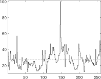
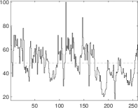
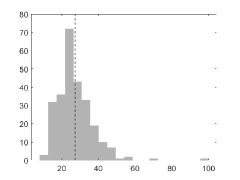
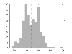
Figure 5: Time series (top) and histograms (bottom) of the global Google search of the words “Climate Change” (left) and “Global Warming” (right). Weekly frequency from 4th December 2016 to 21st November 2021. Empirical mean (dashed line).

(a) Google search dataset “Climate Change”
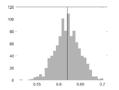
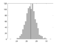
(b) Google search dataset “Global Warming”

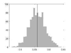
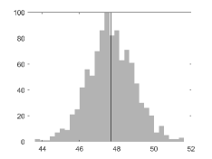
Figure 6: Posterior approximation of the persistence parameter $\alpha$ (left) and the unconditional moment $\mu_{\varepsilon}/(1-\alpha)$ (right) for the global search volume.

4.2 Estimation results

The posterior distribution of the autoregressive coefficient is given in Fig. 6. The coefficient estimate and posterior credible interval (in parenthesis) are $\widehat{\alpha}=0.56$ $(0.50,0.62)$ and $\widehat{\alpha}=0.62$ $(0.56,0.67)$ for the GW and the CC dataset, respectively. This result indicates that the public concern in climate risk is persistent over time worldwide at an aggregate level. The estimated parameter of the innovation process and their 0.95% credible intervals (in parenthesis) are $\widehat{a}=3.53$ $(1.56,6.08)$, $\widehat{b}=0.04$ $(0.01,0.11)$, $\widehat{c}=0.21$ $(0.05,0.47)$ and $\widehat{\beta}=0.48$ $(0.20,0.65)$ for the GW dataset and $\widehat{a}=3.26$ $(1.44,5.72)$, $\widehat{b}=0.12$ $(0.021,0.310)$, $\widehat{c}=0.26$ $(0.032,0.726)$ and $\widehat{\beta}=0.35$ $(0.067,0.623)$ for the CC one. The results indicate a deviation from the Negative Binomial model, thus we apply the DIC criterion $DIC=-4\mathbb{E}(\log p(X|\theta)|y)+2\log p(X|\widehat{\theta})$ to compare GLK-INAR(1) and NB-INAR(1). The $DIC$ is computed following (Spiegelhalter et al.,, 2002):

$$\hbox{DIC}=-4\frac{1}{N}\sum_{j=1}^{N}\log p(X|\theta^{(j)})+2\log p(X|\widehat{\theta})$$ (31)

where $p(X|\theta)$ is the likelihood of the model, $\theta^{(j)}$ $j=1,\ldots,N$ the MCMC draws after thinning and burn-in sample removal, and $\widehat{\theta}$ is the parameter estimate. The DICs for the GLK (NB) INARs fitted on the aggregate CC and GW series are $1.6677\cdot 10^{3}$ $(1.6861\cdot 10^{3})$ and $1.8638\cdot 10^{3}$ $(1.8835\cdot 10^{3})$, respectively.

We run the analysis at a disaggregate level. The results are given in Fig. 7-8 and Tab. 2-3. Figure 7 provides evidence of an inverse relationship between estimated persistence $\widehat{\alpha}$ and dispersion $\widehat{VMR}$ cross countries (reference lines in the left plot). There is evidence of this inverse relationship in both the CC (blue dots) and GW (red dots) datasets. The plot on the right indicates an inverse (direct) relationship between the estimated unconditional mean $\widehat{\mu_{\varepsilon}}/(1-\widehat{\alpha})$ and the dispersion index $\widehat{VMR}$ for the GW (CC). We indicate the parameter estimates for the world volume of searches (stars) in the same picture.

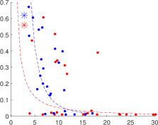
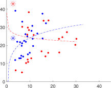
Figure 7: Persistence-dispersion ($\widehat{\alpha}$ and $\widehat{VMR}$, left) and unconditional mean and dispersion ($\widehat{\mu_{\varepsilon}}/(1-\widehat{\alpha})$ and $\widehat{VMR}$, right) scatter plots for all countries in the “Climate Change” (blue) and “Global Warming” (red) datasets. Only countries with less than 21% of zeros are reported. Stars indicate the parameters of the world volume of searches. “*” indicates the parameter estimates for the aggregated search volume.

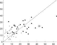
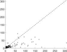
Figure 8: Unconditional mean (left) and dispersion index (right) of the GW (horizontal) and CC (vertical) for countries with more than 21% of zeros (gray dots) less then 21% (black dots) in the number of searches. In each plot the 45^∘ reference line.

	Climate Change dataset				Climate Warming dataset
Country	$\widehat{\alpha}$	$CI$	GLK	LK	$\widehat{\alpha}$	$CI$	GLK	LK
Australia	0.547	(0.501,0.589)	-882.43∗	-885.87	0.343	(0.287,0.397)	-1125.99	-1120.90∗
Bangladesh	0.018	(0.002,0.053)	-1118.68	-1111.99∗	0.001	(0.001,0.005)	-1166.74	-1162.50∗
Brazil	0.011	(0.001,0.029)	-1187.96	-1165.17∗	0.001	(0.001,0.002)	-1027.29	-1024.77∗
Canada	0.672	(0.615,0.714)	-711.55∗	-716.70	0.512	(0.468,0.554)	-1003.35	-1000.60∗
Emirates	0.010	(0.001,0.029)	-1200.72	-1182.74∗	0.005	(0.001,0.020)	-1158.09	-1149.59∗
France	0.184	(0.127,0.248)	-1069.66	-1068.36∗	0.006	(0.001,0.019)	-1140.59	-1130.91∗
Germany	0.298	(0.209,0.373)	-1023.87	-1022.87∗	0.021	(0.001,0.060)	-1099.04	-1094.57∗
India	0.499	(0.420,0.562)	-922.74∗	-923.57	0.482	(0.417,0.541)	-1019.07	-1018.57∗
Indonesia	0.021	(0.003,0.064)	-1123.06	-1108.15∗	0.253	(0.193,0.311)	-1195.34	-1172.30∗
Ireland	0.333	(0.279,0.388)	-953.35	-952.64∗	0.001	(0.001,0.002)	-1093.97	-1094.39∗
Italy	0.169	(0.090,0.241)	-983.83	-982.26∗	0.001	(0.001,0.004)	-1036.21	-1034.28∗
Malaysia	0.002	(0.001,0.008)	-1171.22	-1167.40∗	0.006	(0.001,0.031)	-1135.02	-1129.73∗
Mexico	0.009	(0.001,0.031)	-1160.49	-1148.85∗	0.001	(0.001,0.001)	-1098.96	-1097.73∗
Netherlands	0.148	(0.075,0.218)	-1064.29	-1061.30∗	0.001	(0.001,0.005)	-1066.26	-1059.54∗
NewZealand	0.353	(0.283,0.412)	-894.23∗	-895.29	0.013	(0.001,0.044)	-1151.01	-1136.31∗
Nigeria	0.129	(0.068,0.191)	-1043.77	-1041.80∗	0.017	(0.001,0.062)	-974.18	-966.83∗
Pakistan	0.212	(0.148,0.272)	-1131.60∗	-1124.74	0.023	(0.001,0.064)	-1135.66	-1128.55∗
Philippine	0.409	(0.354,0.460)	-1069.39	-1066.66∗	0.383	(0.327,0.432)	-1150.86	-1138.26∗
Singapore	0.159	(0.095,0.222)	-1099.02	-1094.02∗	0.006	(0.001,0.023)	-1132.94	-1122.04∗
SouthAfrica	0.413	(0.353,0.467)	-923.33∗	-925.21	0.334	(0.274,0.391)	-865.23∗	-868.48
Spain	0.253	(0.193,0.320)	-883.65∗	-886.68	0.001	(0.001,0.002)	-1049.48	-1041.62∗
Thailand	0.008	(0.001,0.035)	-1082.74	-1078.49∗	0.004	(0.001,0.012)	-1218.44	-1193.67∗
UK	0.535	(0.486,0.587)	-932.80∗	-937.25	0.319	(0.246,0.388)	-1084.84	-1081.81∗
US	0.601	(0.549,0.649)	-867.57∗	-871.12	0.606	(0.558,0.649)	-941.39∗	-942.22
Vietnam	0.003	(0.001,0.012)	-1189.79	-1178.82∗	0.001	(0.001,0.001)	-987.59	-986.21∗

Table 2: Estimated GLK-INAR(1) autoregressive coefficient ($\widehat{\alpha}$) and its 95% credible interval (CI), and marginal likelihood of the GLK-INAR(1) and the INARKF(1) models, for the “Climate Change” and “Global Warming” search volumes in different countries. Countries with less than 21% of zeros in the two series. “*” indicate the model with the largest marginal likelihood.

	Climate Change dataset				Climate Warming dataset
Country	$\widehat{\alpha}$	$CI$	GLK	LK	$\widehat{\alpha}$	$CI$	GLK	LK
Argentina	0.001	(0.001,0.001)	-1022.22∗	-1044.08	0.001	(0.001,0.001)	-803.30∗	-850.10
Austria	0.001	(0.001,0.001)	-1085.17	-1082.50∗	0.001	(0.001,0.001)	-717.08∗	-754.18
Belgium	0.002	(0.001,0.012)	-1141.59	-1136.92∗	0.001	(0.001,0.001)	-879.09∗	-944.73
Colombia	0.001	(0.001,0.002)	-1040.35∗	-1053.91	0.001	(0.001,0.001)	-848.15∗	-882.50
Denmark	0.008	(0.001,0.023)	-1123.97	-1101.34∗	0.002	(0.001,0.005)	-973.88	-950.20∗
Egypt	0.001	(0.001,0.002)	-1103.36∗	-1114.87	0.001	(0.001,0.002)	-855.84∗	-867.85
Ethiopia	0.002	(0.001,0.011)	-1089.74	-1081.68∗	0.001	(0.001,0.001)	-876.11∗	-914.27
Finland	0.027	(0.001,0.084)	-987.30	-983.16∗	0.001	(0.001,0.001)	-670.46∗	-679.12
Ghana	0.003	(0.001,0.012)	-992.09	-980.8∗3	0.001	(0.001,0.001)	-854.44∗	-922.58
Jamaica	0.001	(0.001,0.005)	-995.13	-994.24∗	0.001	(0.001,0.001)	-900.84∗	-947.66
Greece	0.001	(0.001,0.001)	-1070.08∗	-1095.69	0.001	(0.001,0.001)	-620.97∗	-687.79
HongKong	0.005	(0.001,0.040)	-1116.20	-1104.70∗	0.001	(0.001,0.001)	-1070.33∗	-1076.02
Iran	0.001	(0.001,0.002)	-1046.05∗	-1107.53	0.001	(0.001,0.002)	-945.79∗	-992.93
Israel	0.001	(0.001,0.001)	-914.20∗	-959.02	0.001	(0.001,0.001)	-726.50∗	-797.23
Japan	0.008	(0.001,0.026)	-1209.16	-1193.53∗	0.002	(0.001,0.004)	-1099.15∗	-1109.15
Kenya	0.104	(0.049,0.170)	-1100.01	-1092.16∗	0.001	(0.001,0.001)	-1073.55∗	-1096.71
Lebanon	0.001	(0.001,0.001)	-761.11∗	-776.44	0.001	(0.001,0.001)	-800.14∗	-850.50
Morocco	0.001	(0.001,0.001)	-755.97∗	-839.02	0.001	(0.001,0.002)	-471.85∗	-534.09
Mauritius	0.001	(0.001,0.002)	-887.72∗	-926.89	0.001	(0.001,0.001)	-601.12∗	-655.86
Myanmar	0.001	(0.001,0.001)	-917.99∗	-979.43	0.001	(0.001,0.002)	-602.14∗	-665.81
Nepal	0.001	(0.001,0.001)	-1148.05	-1145.39∗	0.001	(0.001,0.001)	-1027.36∗	-1060.00
Norway	0.016	(0.003,0.051)	-1121.71	-1105.17∗	0.001	(0.001,0.001)	-1002.83∗	-1004.64
Peru	0.001	(0.001,0.001)	-915.67∗	-950.87	0.001	(0.001,0.001)	-666.93∗	-712.80
Polish	0.001	(0.001,0.001)	-1078.86∗	-1090.00	0.001	(0.001,0.001)	-1000.76∗	-1063.99
Portugal	0.002	(0.001,0.010)	-1035.62	-1030.57∗	0.001	(0.001,0.001)	-800.35∗	-851.13
Qatar	0.001	(0.001,0.001)	-879.41∗	-917.09	0.001	(0.001,0.001)	-674.32∗	-701.04
Romania	0.001	(0.001,0.001)	-880.49∗	-901.20	0.001	(0.001,0.001)	-819.31∗	-896.17
Russia	0.001	(0.001,0.003)	-1038.70∗	-1050.47	0.001	(0.001,0.001)	-984.09∗	-1023.75
StHelena	0.001	(0.001,0.001)	-873.70∗	-914.40	0.001	(0.001,0.002)	-374.81∗	-394.04
SouthKorea	0.004	(0.001,0.019)	-1149.02∗	-1142.78	0.001	(0.001,0.003)	-1051.25∗	-1057.01
SriLanka	0.001	(0.001,0.001)	-1086.31∗	-1109.74	0.001	(0.001,0.003)	-842.37∗	-863.17
Sweden	0.136	(0.067,0.205)	-1031.72	-1026.82∗	0.001	(0.001,0.001)	-1078.30∗	-1089.70
Swiss	0.028	(0.005,0.063)	-1055.02	-1046.17∗	0.001	(0.001,0.001)	-835.78∗	-878.17
Taiwan	0.001	(0.001,0.001)	-1074.92∗	-1085.60	0.001	(0.001,0.001)	-794.34∗	-815.63
TrinidadTobago	0.001	(0.001,0.001)	-920.81∗	-955.62	0.001	(0.001,0.001)	-809.94∗	-858.50
Turkey	0.004	(0.001,0.019)	-1095.99	-1091.08∗	0.001	(0.001,0.001)	-1085.46∗	-1091.38
Ukraine	0.001	(0.001,0.001)	-902.24∗	-949.78	0.001	(0.001,0.002)	-709.80∗	-745.82
Hungary	0.001	(0.001,0.001)	-935.84	-953.58∗	0.001	(0.001,0.001)	-642.03∗	-717.52
Zambia	0.001	(0.001,0.003)	-1075.30	-1053.65∗	0.001	(0.001,0.001)	-746.07∗	-789.78
Zimbabwe	0.001	(0.001,0.002)	-1130.16	-1128.73∗	0.001	(0.001,0.002)	-658.24∗	-690.68

Table 3: Estimated GLK-INAR(1) autoregressive coefficient ($\widehat{\alpha}$) and its 95% credible interval (CI), and marginal likelihood of the GLK-INAR(1) and the INARKF(1) models, for the “Climate Change” and “Global Warming” search volumes in different countries. Countries with more than 21% of zeros in the two series. “*” indicate the model with the largest marginal likelihood.

The terms “Climate Change” and “Global Warming” are used interchangeably, nevertheless, they describe different phenomena and can be used to determine the level of understanding of the public about these two parallel concepts Lineman et al., (2015). We investigate the relationships in the search volumes through the lens of our GLK-INAR(1) model. The left plot in Fig. 8 shows the unconditional mean of the search volumes for the two concepts in all countries (dots). In public attention, the two concepts are connected in the long run. We find a positive association for both countries with large (percentage of zeros $<$ 21%) and low search volumes (percentage of zeros $>$ 21%). There is an asymmetric effect in the overdispersion (right plot), and in all countries, the GW search volume has a larger VMR than the CC volume. This can be explained by the GW larger variability induced by the changes in the use of the GW term in the official communications.

Comparing the coefficients across the rows of Tables 2-3, we find evidence of two types of series, one with high persistence and the other with low persistence. Moreover, for each country the level of persistence is similar across the two datasets (compare columns of Tables 2-3).

Tables 2-3 report the marginal likelihood of the GLK-INAR(1) and Lagrangian Katz INAR(1) in columns GLK and LK respectively. We find evidence of a better fitting of the GLK-INAR(1) for some countries and variables, e.g. CC searches in India and CC and GW searcher in South Africa. In order to get further insights into the results, we study the relationship between the dynamic and dispersion properties of the series and the actual level of climate risk of the countries. We consider the Global Climate Risk Index (CRI), which ranks countries and regions following the impacts of extreme weather events (such as storms, hurricanes, floods, heatwaves, etc.). The lower the index value, the larger the climate risk is. Following the values of the CRI for 2021, based on the events recorded from 2000 to 2019, our dataset includes some of the countries most exposed to the climate risk, such as Japan, Philippines, Germany, South Africa, India, Sri-Lanka and Canada (Eckstein et al.,, 2021, see).

The left plot in Fig. 9 shows unconditional mean against the CRI. There is evidence of a positive relationship between the public interest in climate-related topics and the actual level of climatic risk. Otherwise said, the lower the CRI level, the larger the Google search volumes are (see dashed lines). For example India has high risk (CRI equal to 7) and very high long-run level of public attention.

The right plot reports the coefficient of variation against the CRI for all countries in the “Climate Change” (blue) and “Global Warming” (red) datasets. The dashed lines represent linear regressions estimated on the data. There is evidence of a negative relationship between dispersion of the public concern and climatic risk; that is, in countries with more significant risk levels, the Google search volumes are less over-dispersed.

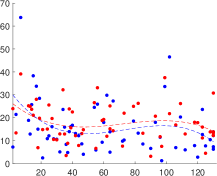
Figure 9: Climate Risk Index and unconditional mean scatter plot (CRI-$\mu_{\varepsilon}/(1-\alpha)$, left) and Climate Risk Index and dispersion scatter plot (CRI-$CV$, right) scatter plots for all countries in the “Climate Change” (blue) and “Global Warming” (red) datasets. Dashed lines represent the linear regression estimated on the data.

5 Conclusion

A novel integer-valued autoregressive process is proposed with Generalized Lagrangian Katz innovations. Theoretical properties of the model, such as stationarity, moments, and semi-self-decomposability are provided. A Bayesian approach to inference is proposed, and an efficient Gibbs sampling procedure has been proposed. The modeling framework is applied to a Google Trend dataset on the public concern about climate change for 65 countries. New evidence is provided about the long-run level of public attention, its persistence and dispersion in countries with low and high level of climate risk.

Appendix A Proof of the results in Section 2

A.1 Proof of the resutls in Remark 1

Following (Consul and Famoye,, 2006, p. 10-11) the general Lagrangian expansion of $f(u)$ is

$$\frac{f(z)}{1-zg^{\prime}/g(z)}=\sum_{j=0}^{\infty}\frac{u^{j}}{j!}\left|\partial^{j}(g^{j}(z)f(z))\right|_{z=0}$$ (32)

where $u$ satisfies $z=ug(z)$. The definition of Lagrangian distribution given in Janardan, (1998) can is obtained from the one given above by replacing $f(z)$ with $f(z)(1-zg^{\prime}(z)/g(z)))$. By applying iteratively the derivative $\partial$ to the product of functions we obtain the coefficient in the $j$-th term of the expansion

$$\frac{1}{j!}|\partial^{j}\left(g(z)^{j}f(z)(1-zg^{\prime}(z)/g(z))\right)|_{z=0}=\frac{1}{j!}|\partial^{j-1}(g(z)^{j}f^{\prime}(z)$$ (33)

$$+(j-1)g^{\prime}(z)g(z)^{j-1}f(z)-z\partial g^{j-1}(z)g^{\prime}(z)f(z))|_{z=0}=\ldots$$ (34)

$$=\frac{1}{j!}|\partial^{j-1}(g(z)^{j}f^{\prime}(z))|_{z=0}+|\partial^{j-\ell}\left((j-\ell)\partial^{\ell-1}(g^{\prime}(z)g(z)^{j-1}f(z))\right.$$ (35)

$$\left.-z\partial^{\ell}(g^{j-1}(z)g^{\prime}(z)f(z))\right)|_{z=0}=\frac{1}{j!}|\partial^{j-1}(g(z)^{j}f^{\prime}(z))|_{z=0}$$ (36)

where we set $\ell=j$ to get the result and the following equivalent Lagrangian expansion

$$\frac{f(z)}{1-zg^{\prime}/g(z)}=\sum_{j=0}^{\infty}\frac{u^{j}}{j!}\left|\partial^{j}(g^{j}(z)f(z))\right|_{z=0}$$ (37)

$$\Leftrightarrow f(z)=\sum_{j=0}^{\infty}\frac{u^{j}}{j!}\left|\partial^{j-1}(g^{j}(z)f^{\prime}(z))\right|_{z=0}$$ (38)

In particular, for $j\geq 1$,

$$p_{j}=\frac{1}{j!}\left|\partial^{j-1}(g^{j}(z)f^{\prime}(z))\right|_{z=0}$$

provided that $p_{j}\geq 0$. Let $f(z)=\left(\frac{1-\beta}{1-\beta z}\right)^{a/c}$ and $g(z)=\left(\frac{1-\beta}{1-\beta z}\right)^{b/c}$ be the transformed and the transformer function, respectively. Then

$$f^{\prime}(z)=\frac{a}{c}\left(\frac{1-\beta}{1-\beta z}\right)^{\frac{a}{c}+1}\frac{\beta}{1-\beta},$$ (39)

$$g^{k}(z)f^{\prime}(z)=\frac{a}{c}\left(\frac{1-\beta}{1-\beta z}\right)^{\frac{a}{c}+k\frac{b}{c}+1}\frac{\beta}{1-\beta}.$$ (40)

Hence

$$p_{0}=f(0)=\left({1-\beta}\right)^{\frac{a}{c}}\quad p_{1}=g^{1}(0)f^{\prime}(0)=\frac{a}{c}\left({1-\beta}\right)^{\frac{a}{c}+\frac{b}{c}}{\beta}.$$

while, for $k\geq 2$, the $k$-th coefficient of the Lagrangian expansion in Eq. 37 is

$$p_{k}=\frac{1}{k!}|\partial^{k-1}(g(z))^{k}f^{\prime}(z)|_{z=0}=\frac{1}{k!}\partial^{k-2}|(\frac{a}{c}\frac{\beta^{2}}{(1-\beta)^{2}}\xi_{k}\left(\frac{1-\beta}{1-\beta z}\right)^{\xi_{k}+1})|_{z=0}$$ (41)

$$=\frac{1}{k!}|\partial^{k-3}(\frac{a}{c}\frac{\beta^{3}}{(1-\beta)^{3}}(\xi_{k}(\xi_{k}+1))\left(\frac{1-\beta}{1-\beta z}\right)^{\xi_{k}+2})|_{z=0}$$ (42)

$$=...$$ (43)

$$=\frac{1}{k!}\beta^{k}\frac{a}{c}(1-\beta)^{\frac{a}{c}+k\frac{b}{c}}\prod_{m=0}^{k-2}\left(\xi_{k}+m\right)$$ (44)

$$=\frac{1}{k!}\beta^{k}\frac{a}{c}(1-\beta)^{\frac{a}{c}+k\frac{b}{c}}\prod_{m=1}^{k-1}\left(\frac{a}{c}+k\frac{b}{c}+m\right)$$ (45)

$$=\frac{1}{k!}\beta^{k}\frac{a}{c}(1-\beta)^{\frac{a}{c}+k\frac{b}{c}}\left(\frac{a}{c}+k\frac{b}{c}+1\right)_{{k-1}\uparrow}$$ (46)

$$=\frac{1}{k!}\beta^{k}\frac{a}{c}\frac{1}{(\frac{a}{c}+k\frac{b}{c}+k)}(1-\beta)^{\frac{a}{c}+k\frac{b}{c}}\left(\frac{a}{c}+k\frac{b}{c}+1\right)_{{k}\uparrow}$$ (47)

where $\xi_{k}=\frac{a}{c}+k\frac{b}{c}+1$ and $(x)_{{k}\uparrow}=x(x+1)\ldots(x+k-1)$ is the rising factorial.

• If $a>0,b>0,c>0$ one has $p_{k}>0$ for every $k\geq 1$.

• If $-c<b<0$, $a/c,b/c\in\mathbb{N}$ and $(c-a)/(c+b)\leq(a+c)/|b|$, then for $k<k^{*}=(a+c)/|b|$ one has

  $$\frac{a+bk}{c}+1>0$$

  and hence also

  $$\prod_{m=1}^{k-1}\left(\frac{a}{c}+k\frac{b}{c}+m\right)>0$$

  proving that $p_{k}>0$. For $k\geq k^{*}\geq(c-a)/(c+b)$ one has that $m_{k}=(|b|k-a)/c$ is an integer with $1\leq m_{k}\leq k-1$ and hence the product $\prod_{m=1}^{k-1}\left(\frac{a}{c}+k\frac{b}{c}+m\right)=0$ since for $m=m_{k}$ one has $\frac{a}{c}+k\frac{b}{c}+m=0$. This shows that $p_{k}=0$ for every $k\geq k^{*}$.

A.2 Proof of the results in Remark 3

Replacing $c$ by $\beta$ one obtains a Lagrangian Katz distribution. The LK is one of the few distributions which admits more pgfs. Let us consider the following definition of pgf for a $\mathcal{LK}(a,b,\beta)$

$$G(u,a,b,\beta)=\left(\frac{1-\beta z}{1-\beta}\right)^{-\frac{a}{\beta}},\quad\hbox{with}\,\,z(a,b,\beta)=u\left(\frac{1-\beta z}{1-\beta}\right)^{-\frac{b}{\beta}}.$$ (49)

given in (Consul and Famoye,, 2006, p. 241). Defining $n=(1-\beta z)/(\beta(z-1))$ and $1/\beta=n(z-1)+z$ the limiting pgf becomes

$$\underset{\beta\rightarrow 0^{+}}{\lim}G(u;a,b,\beta)=\underset{n\rightarrow+\infty}{\lim}\left(1+\frac{1}{n}\right)^{\frac{n(z-1)+z}{a}}=e^{a(z-1)},$$ (50)

with

$$\underset{\beta\rightarrow 0^{+}}{\lim}z(a,b,\beta)=\underset{n\rightarrow+\infty}{\lim}\left(1+\frac{1}{n}\right)^{\frac{n(z-1)+z}{b}}=e^{b(z-1)}$$ (51)

which is the pgf of a GP given in (Consul and Famoye,, 2006, pp. 166).

A.3 Proof of the results in Theorem 2

A random variable $X$ is infinite divisible if for every $n\in\mathbb{N}$ there exists a sequence of random variables $X_{nj}$, $j=1,\ldots,n$ such that $X$ has the same distribution of $X_{n1}+\ldots+X_{nn}$. From the pgf of a GLK given in Eq. 4

$$\mathbb{E}(X)=\mathbb{E}\left(u^{X}\right)=\left(\frac{1-\beta}{1-\beta z}\right)^{\frac{a}{c}}=\prod_{j=1}^{n}\left(\frac{1-\beta}{1-\beta z}\right)^{\frac{a}{nc}}$$ (52)

which is the pgf of the sum of $n$ independent GLKs with distribution $\mathcal{GLK}(a/n,b,c,\beta)$ where $a/n>0$ according to the definition of GLK.

A.4 Proofs of Equations (10)-(9)

Before proving the general result let us prove the following two properties of the thinning operator

1. $\alpha\circ(\alpha\circ X)=\alpha^{2}\circ X$

2. $\alpha\circ(X+Y)=\alpha\circ X+\alpha\circ Y$

where $X$ and $Y$ are two independent discrete-valued random variables. Property (i) follows from the law of iterated expectations and the properties of the probability generating function (pgf):

$$\mathbb{E}(\varphi^{\alpha\circ(\alpha\circ X)})=\mathbb{E}(\mathbb{E}(\varphi^{\alpha\circ(\alpha\circ X)}|\alpha\circ X))=\mathbb{E}(\prod_{j=1}^{\alpha\circ X}\mathbb{E}(\varphi^{B_{j}}|\alpha\circ X))$$ (53)

$$=\mathbb{E}(((1-\alpha)+\varphi\alpha)^{(\alpha\circ X)})=((1-\alpha)+((1-\alpha)+\varphi\alpha)\alpha)^{X}$$ (54)

$$=(1-\alpha^{2}+\varphi\alpha^{2})^{X}=\mathbb{E}(\varphi^{\alpha^{2}\circ X})$$ (55)

which is the pgf of the r.v. $\alpha^{2}\circ X$. Property (ii) follows from:

$$\alpha\circ(X+Y)=\sum_{j=1}^{X+Y}B_{j}=\sum_{j=1}^{X}B_{j}+\sum_{j=X+1}^{X+Y}B_{j}$$ (56)

$$=\alpha\circ X+\sum_{l=1}^{Y}\tilde{B}_{l}=\alpha\circ X+\alpha\circ Y$$ (57)

where we defined $\tilde{B}_{l}=B_{l+X}$ for $l=1,\ldots,Y$. Applying iteratively the two properties of the binomial thinning operator returns the following representation

$$X_{t+k}=\alpha\circ X_{t+k-1}+\varepsilon_{t+k}=\alpha^{2}\circ X_{t+k-2}+\alpha\circ\varepsilon_{t+k-1}+\varepsilon_{t+k}$$ (58)

$$=\ldots=\alpha^{k}\circ X_{t}+\sum_{j=0}^{k-1}\alpha^{j}\circ\varepsilon_{t+1-j}$$ (59)

where we defined $\alpha^{0}\circ X=X$.

The conditional pgf follows from the above decomposition

$$H_{X_{t+k}|X_{t}}(u)=\mathbb{E}(u^{X_{t+k}}|X_{t})=\mathbb{E}(u^{\alpha^{k}\circ X_{t}}|X_{t})\prod_{j=0}^{k-1}\mathbb{E}(u^{\alpha^{j}\circ\varepsilon_{t+1-j}})$$ (60)

$$=(1-\alpha^{k}+\alpha^{k}u)^{X_{t}}\prod_{j=0}^{k-1}H(1-\alpha^{j}+\alpha^{j}u)$$ (61)

where $H(u)$ satisfies Eq. 3 and 4.

A.5 Proof of the results in Theorem 1

Using the expressions for the moments given in Th. 1 and the independent assumption of the innovations on the thinning and on the past values of process one obtains for the case $k=1$

$$\mathbb{E}(\alpha\circ X_{t}+\varepsilon_{t+1}|X_{t})=\mathbb{E}(\sum_{i=1}^{X_{t}}B_{it}+\varepsilon_{t+1}|X_{t})$$ (62)

$$=\alpha X_{t}+\mathbb{E}(\varepsilon_{t+1})=\alpha X_{t}+\frac{a\theta}{\kappa}$$ (63)

and

$$\mathbb{V}(\alpha\circ X_{t}+\varepsilon_{t+1}|X_{t})=\mathbb{V}(\sum_{i=1}^{X_{t}}B_{it}|X_{t})+\mathbb{V}(\varepsilon_{t+1})$$ (64)

$$=X_{t}(\alpha-\alpha^{2})+\frac{a(1-\beta)\theta}{\kappa^{3}}$$ (65)

Following the recursive representation in 58 and by independence assumption, the conditional variance writes as

$$\mathbb{E}(\alpha\circ X_{t+k}|X_{t})=\mathbb{E}(\alpha^{k}\circ X_{t}+\sum_{j=0}^{k-1}\alpha^{j}\circ\varepsilon_{t+1-j}|X_{t})$$ (66)

$$=\alpha^{k}X_{t}+\frac{1-\alpha^{k-1}}{1-\alpha}\frac{a\theta}{\kappa}$$ (67)

where we defined $\alpha^{0}\circ X=X$. Similarly, the conditional variance writes as

$$\mathbb{V}(\alpha\circ X_{t+k}|X_{t})=\mathbb{V}(\alpha^{k}\circ X_{t}+\sum_{j=0}^{k-1}\alpha^{j}\circ\varepsilon_{t+1-j}|X_{t})$$ (68)

$$=\mathbb{V}(\alpha^{k}\circ X_{t}|X_{t})+\mathbb{V}(\sum_{j=0}^{k-1}\alpha^{j}\circ\varepsilon_{t+1-j})$$ (69)

$$=(\alpha^{k}-\alpha^{2k})X_{t}+\sum_{j=0}^{k-1}(\mathbb{V}(\mathbb{E}(\alpha^{j}\circ\varepsilon_{t+1-j}|\varepsilon_{t+1-j}))+\mathbb{E}(\mathbb{V}(\alpha^{j}\circ\varepsilon_{t+1-j}|\varepsilon_{t+1-j})))$$ (70)

$$=(\alpha^{k}-\alpha^{2k})X_{t}+\sum_{j=0}^{k-1}(\alpha^{2j}\frac{a(1-\beta)\theta}{\kappa^{3}}+(\alpha^{j}-\alpha^{2j}))\frac{a\theta}{\kappa})$$ (71)

$$=(\alpha^{k}-\alpha^{2k})X_{t}+\frac{1-\alpha^{2k}}{1-\alpha^{2}}\left(\frac{a(1-\beta)\theta}{\kappa^{3}}-\frac{a\theta}{\kappa}\right)+\frac{1-\alpha^{k}}{1-\alpha}\frac{a\theta}{\kappa}$$ (72)

A.6 Proof of the result in Remark 5

Setting $b=0$, $c=\beta=\theta_{1}$ and $a=\theta_{2}$, it follows $\kappa=1-\theta_{2}$ and $\theta=1$, thus the conditional mean and variance become

$$\alpha^{k}X_{t}+\frac{1-\alpha^{k-1}}{1-\alpha}\frac{a\theta}{\kappa}=\alpha^{k}X_{t}+\frac{1-\alpha^{k-1}}{1-\alpha}\frac{\theta_{1}}{1-\theta_{2}}$$ (73)

and

$$(\alpha^{k}-\alpha^{2k})X_{t}+\frac{1-\alpha^{2k}}{1-\alpha^{2}}\left(\frac{a(1-\beta)\theta}{\kappa^{3}}-\frac{a\theta}{\kappa}\right)+\frac{1-\alpha^{k}}{1-\alpha}\frac{a\theta}{\kappa}$$ (74)

$$=(\alpha^{k}-\alpha^{2k})X_{t}+\frac{1-\alpha^{2k}}{1-\alpha^{2}}\left(\frac{\theta_{1}(1-\theta_{2})}{(1-\theta_{2})^{3}}-\frac{\theta_{1}}{(1-\theta_{2})}\right)+\frac{1-\alpha^{k}}{1-\alpha}\frac{\theta_{1}}{(1-\theta_{2})}$$ (75)

$$=(\alpha^{k}-\alpha^{2k})X_{t}+\frac{1-\alpha^{2k}}{1-\alpha^{2}}\frac{\theta_{1}}{(1-\theta_{2})^{2}}+\frac{\theta_{1}}{(1-\theta_{2})}\left(\frac{1-\alpha^{k}}{1-\alpha}-\frac{1-\alpha^{2k}}{1-\alpha^{2}}\right)$$ (76)

$$=(\alpha^{k}-\alpha^{2k})X_{t}+\frac{1-\alpha^{2k}}{1-\alpha^{2}}\frac{\theta_{1}}{(1-\theta_{2})^{2}}+\frac{\theta_{1}}{(1-\theta_{2})}\frac{(1-\alpha^{k})(1+\alpha-1-\alpha^{k})}{1-\alpha^{2}}$$ (77)

A.7 Proof of the result in Remark 6

Under the assumption $|\alpha|<1$ the limiting conditional variance becomes:

$$\frac{1}{1-\alpha^{2}}\left(\frac{a(1-\beta)\theta}{\kappa^{3}}-\frac{a\theta}{\kappa}+\frac{a\theta(1+\alpha)}{\kappa}\right)$$ (78)

$$\frac{1}{1-\alpha^{2}}\left(\frac{a(1-\beta)\theta}{\kappa^{3}}-\frac{a\theta-a\theta(1+\alpha)}{\kappa}\right)$$ (79)

$$\frac{1}{1-\alpha^{2}}\left(\frac{a(1-\beta)\theta}{\kappa^{3}}+\frac{a\theta\alpha}{\kappa}\right)$$ (80)

$$\frac{1}{1-\alpha^{2}}\frac{a\theta}{\kappa^{3}}\left((1-\beta)+\alpha\kappa^{2}\right)$$ (81)

A.8 Proof of the results in Theorem 2

We follow the same argument as in Bourguignon and Vasconcellos, (2015). Let $p_{l,k}=\mathbb{P}(X_{t}=k|X_{t-1}=l)$ be the transition probability given in Eq. 2.2. The process is irreducible since that every $k\in\mathbb{N}$ can be reached from every $l\in\mathbb{N}$. The transition are constant over $t$, thus the process admits a stationary distribution. We need to show that

$$\underset{t\rightarrow\infty}{\lim}\frac{1}{t}\sum_{m=1}^{t}P_{0,0}^{m}>0$$ (82)

and bounded.

Next we show by induction that

$$P^{m}_{x,0}=p_{0}(1-\alpha^{m})^{x}\prod_{j=1}^{m-1}H(1-\alpha^{j})$$ (83)

where

$$H(1-\alpha^{j})=\sum_{z=0}^{\infty}p_{z}(1-\alpha^{j})^{z}.$$ (84)

For $m=1$ the equation is satisfied since

$$P^{1}_{x,0}=p_{0}(1-\alpha)^{x}.$$ (85)

Assume it is satisfied for $m$ then for $m+1$ we have

$$P^{m+1}_{x,0}=\sum_{z=0}^{\infty}P^{1}_{x,z}P^{m}_{z,0}$$ (86)

$$=\sum_{z=0}^{\infty}\sum_{k=0}^{\min(x,z)}{x\choose k}\alpha^{k}(1-\alpha)^{x-k}p_{z-k}P^{m}_{z,0}$$ (87)

$$=\sum_{k=0}^{x}{x\choose k}\alpha^{k}(1-\alpha)^{x-k}\sum_{z=k}^{\infty}p_{z-k}P^{m}_{z,0}$$ (88)

$$=\sum_{k=0}^{x}{x\choose k}\alpha^{k}(1-\alpha)^{x-k}\sum_{z=0}^{\infty}p_{z}P^{m}_{z+k,0}$$ (89)

$$=\sum_{k=0}^{x}{x\choose k}\alpha^{k}(1-\alpha)^{x-k}p_{0}(1-\alpha^{m})^{k}\sum_{z=0}^{\infty}p_{z}(1-\alpha^{m})^{z}$$ (90)

$$=\sum_{k=0}^{x}{x\choose k}\alpha^{k}(1-\alpha)^{x-k}\sum_{z=0}^{\infty}p_{z}p_{0}(1-\alpha^{m})^{z+k}\prod_{j=1}^{m-1}H(1-\alpha^{j})$$ (91)

$$=p_{0}\prod_{j=1}^{m-1}H(1-\alpha^{j})\sum_{k=0}^{x}{x\choose k}\alpha^{k}(1-\alpha)^{x-k}(1-\alpha^{m})^{k}\sum_{z=0}^{\infty}p_{z}(1-\alpha^{m})^{z}$$ (92)

$$=p_{0}\prod_{j=1}^{m-1}H(1-\alpha^{j})\sum_{k=0}^{x}{x\choose k}\alpha^{k}(1-\alpha)^{x-k}(1-\alpha^{m})^{k}H(1-\alpha^{m})$$ (93)

$$=p_{0}\prod_{j=1}^{m}H(1-\alpha^{j})\sum_{k=0}^{\min(x,z)}{x\choose k}\alpha^{k}((1-\alpha^{m})/(1-\alpha))^{k}(1-\alpha)^{x}$$ (94)

where $p_{x}$ is the pmf of the GLK and the summation in the last line is the pgf of the GLK. It follows that

$$P^{m+1}_{x,0}=p_{0}\prod_{j=1}^{m}H(1-\alpha^{j})\sum_{k=0}^{\min(x,z)}{x\choose k}\alpha^{k}((1-\alpha^{m})/(1-\alpha))^{k}(1-\alpha)^{x}$$ (96)

$$P^{m+1}_{x,0}=p_{0}\prod_{j=1}^{m}H(1-\alpha^{j})\sum_{k=0}^{\min(x,z)}{x\choose k}\alpha^{k}(1+\alpha+\ldots+\alpha^{m})^{k}(1-\alpha)^{x}$$ (97)

$$=p_{0}(1-\alpha)^{x}(1+\alpha+\ldots+\alpha^{m-1})^{x}\prod_{j=1}^{m}H(1-\alpha^{j})$$ (98)

$$=p_{0}(1-\alpha^{m+1})^{x}\prod_{j=1}^{m}H(1-\alpha^{j})$$ (99)

Consider the logarithm

$$\log(P^{m+1}_{0,0})=\log p_{0}+\sum_{j=1}^{m}\log H(1-\alpha^{j})=\log p_{0}+\sum_{j=1}^{m}\log(1+H(1-\alpha^{j})-1).$$

Now, recalling that $0<\alpha<1$, one has $0\geq H(1-\alpha^{j})-1\geq H(1-\alpha)-1=:-k_{\alpha}>-1$ for every $j\geq 1$. Since, by Taylor expansion, for every $|z|\leq k_{\alpha}<1$,

$$|\log(1+z)|\leq|z|+C|z|^{2}$$

for a suitable constant $C=C(k_{\alpha})$, then

$$|\log(P^{m+1}_{0,0})|\leq|\log p_{0}|+\sum_{j=1}^{m}\Big{(}|H(1-\alpha^{j})-1|+C|H(1-\alpha^{j})-1|^{2}).$$

Note that

$$1-H(1-\alpha^{j})=H(1)-H(1-\alpha^{j})=(-\alpha^{j})\dot{H}(\xi_{\alpha})$$

for some $\xi_{\alpha}\in((1-\alpha^{j}),1)$. Now for any $x\in(0,1)$

$$\dot{H}(x)=\sum_{z\geq 1}zx^{z-1}p_{z}\leq\sum_{z\geq 1}zp_{z}=:M_{1}$$

since the GLK distribution has finte first moment. Hence one gets

$$|H(1-\alpha^{j})-1|\leq\alpha^{j}M_{1}$$

and

$$|\log(P^{m+1}_{0,0})|\leq|\log p_{0}|+\sum_{j\geq 1}\Big{(}M_{1}\alpha^{j}+CM_{1}^{2}\alpha^{2j}\Big{)}<+\infty$$

since $\alpha\in(0,1)$.

Remark 8.

We note that the proof only uses the fact that

$$X_{t+1}=\alpha\circ X_{t}+\varepsilon_{t}$$

with $E[\varepsilon_{t}]<+\infty$.

A.9 Proof of the results in Theorem 5

(i) Under stationarity assumption one has $\mu_{X}=E(X_{s})$ for all $s\in\mathbb{Z}$, thus $\mu_{X}=\alpha\mu_{X}+\mathbb{E}(\varepsilon_{t})$ which implies $\mu_{X}=\mu_{\varepsilon}/(1-\alpha)$.

(ii) Let $\mu_{X}^{(2)}=E(X_{s}^{2})$ for all $s\in\mathbb{Z}$, then $\mathbb{E}(X_{t}^{2})=\mathbb{E}((\alpha\circ X_{t-1})^{2})+\mathbb{E}(\varepsilon_{t}^{2})+\mathbb{E}(2(\alpha\circ X_{t-1})\varepsilon_{t})=$ $\mathbb{V}((\alpha\circ X_{t-1})^{2})+(\mathbb{E}(\alpha\circ X_{t-1}))^{2}+\mathbb{E}(\varepsilon_{t}^{2})+\mathbb{E}(2(\alpha\circ X_{t-1})\varepsilon_{t})$. By the law of iterated expectation

$$\mu_{X}^{(2)}=\alpha^{2}(\mu_{X}^{(2)}-\mu_{X}^{2})+\alpha(1-\alpha)\mu_{X}+\alpha^{2}\mu_{X}^{2}+\mu_{\varepsilon}^{(2)}+\alpha\mu_{X}\mu_{\varepsilon}$$ (100)

$$\Leftrightarrow\mu_{X}^{(2)}=\frac{1}{1-\alpha^{2}}\left(\alpha\mu_{\varepsilon}+\mu_{\varepsilon}^{(2)}+\frac{2\alpha}{1-\alpha}\mu_{\varepsilon}^{2}\right)$$ (101)

From (i) and (ii) one can obtain the unconditional variance

$$\sigma_{X}^{2}=\mu_{X}^{(2)}-\mu_{X}^{2}$$ (102)

$$=\sigma_{X}^{2}=\frac{1}{1-\alpha^{2}}\left(\alpha\mu_{\varepsilon}+\mu_{\varepsilon}^{(2)}+\frac{2\alpha}{1-\alpha}\mu_{\varepsilon}^{2}\right)-\frac{1}{(1-\alpha)^{2}}\mu_{\varepsilon}^{2}$$ (103)

$$=\frac{1}{1-\alpha^{2}}\left(\alpha\mu_{\varepsilon}+\mu_{\varepsilon}^{(2)}+\frac{2\alpha}{1-\alpha}\mu_{\varepsilon}^{2}-\frac{1+\alpha}{(1-\alpha)}\mu_{\varepsilon}^{2}\right)$$ (104)

$$=\frac{1}{1-\alpha^{2}}\left(\alpha\mu_{\varepsilon}+\sigma^{2}_{\varepsilon}\right)$$ (105)

From (i) and (ii) one can obtain the unconditional variance

$$\sigma_{X}^{2}=\mu_{X}^{(2)}-\mu_{X}^{2}$$ (106)

$$=\frac{1}{1-\alpha^{2}}\left(\alpha\mu_{\varepsilon}+\sigma^{2}_{\varepsilon}\right)-\frac{1}{(1-\alpha)^{2}}\mu_{\varepsilon}^{2}$$ (107)

$$=\frac{1}{(1-\alpha^{2})(1-\alpha)}\left(\alpha(1-\alpha)\mu_{\varepsilon}+(1-\alpha)\sigma^{2}_{\varepsilon}-(1+\alpha)\mu_{\varepsilon}^{2}\right)$$ (108)

$$=\frac{1}{(1-\alpha^{2})}\left(\alpha\mu_{\varepsilon}+\sigma^{2}_{\varepsilon}/(1-\alpha)-\mu_{\varepsilon}^{2}\right)$$ (109)

(iii) $\mathbb{E}(X_{t}X_{t-k})=\mathbb{E}((\alpha\circ X_{t-1}+\varepsilon_{t})X_{t-k})=$ $\mathbb{E}(\mathbb{E}((\alpha\circ X_{t-1})X_{t-k}|X_{t-k},X_{t-1}))+\mathbb{E}(\varepsilon_{t})\mathbb{E}(X_{t-k})=\alpha\mathbb{E}(X_{t-1}X_{t-k})+\mu_{\varepsilon}\mu_{X}$. From (i) and (iii) and stationarity $\mathbb{C}ov(X_{t},X_{t-k})=\gamma_{k}$ for all $t\in\mathbb{Z}$ one obtains the autocorrelation function

$$\mathbb{C}ov(X_{t},X_{t-k})=\mathbb{E}(X_{t}X_{t-k})-\mathbb{E}(X_{t})\mathbb{E}(X_{t-k})$$ (111)

$$=\alpha\mathbb{E}(X_{t-1}X_{t-k})+\mu_{\varepsilon}\mu_{X}-(\alpha\mathbb{E}(X_{t-1})+\mu_{\varepsilon})\mu_{X}$$ (112)

$$=\alpha\mathbb{C}ov(X_{t-1}X_{t-k})=\alpha\gamma_{k}=\alpha^{2}\gamma_{k-2}=\cdots=\alpha^{k}\sigma^{2}_{X}$$ (113)

(iii) Let us denote with $(x)_{m}=x(x-1)\ldots(x-m+1)$ the falling factorial and with $\mu^{(\underline{k})}=\mathbb{E}((X)_{k})$ the $m$-order falling factorial moment of a random variable $X$. The following two results will be used. The relationships between non-central moments and falling factorial moments are

$$\mathbb{E}(X_{t}^{m}) = \sum_{k=0}^{m}S(m,k)\mathbb{E}((X_{t})_{k})$$ (114)

$$\mathbb{E}((X_{t})_{m}) = \sum_{k=0}^{m}s(m,k)\mathbb{E}(X_{t}^{k})$$ (115)

where $s(m,k)$ and $S(m,k)$ are the Stirling numbers of the I and II kind, respectively (e.g., see Consul and Famoye,, 2006, p. 18). Let $X$ and $Y$ be two random variables then

$$\mathbb{E}((X+Y)_{m})=\sum_{k=0}^{m}{m\choose k}\mathbb{E}((X)_{k})\mathbb{E}((X)_{m-k})$$ (116)

which can be proved by induction. Let $\alpha\circ X$ a binomial thinning with $X$ a discrete random variable, then

$$\mathbb{E}((\alpha\circ X)_{k})=\mathbb{E}((\sum_{j=1}^{X}B_{j})_{k})=\mathbb{E}\left(\sum_{|\kappa|=k}\prod_{j=1}^{X}B_{j}^{\kappa_{j}}\right)=\mathbb{E}\left({X\choose k}k!\alpha^{k}\right)=\alpha^{k}\mathbb{E}((X)_{k})$$ (117)

where $|\kappa|=\kappa_{1}+\ldots+\kappa_{X}$. Using the results given above and stationarity (i.e. $\mathbb{E}((X_{t})_{m})=\mu_{X}^{(\underline{m})}$ one obtains

$$\mathbb{E}((X_{t})_{m})=\mathbb{E}((\alpha\circ X_{t-1}+\varepsilon_{t})_{m})$$ (118)

$$=\sum_{k=0}^{m}{m\choose k}\mathbb{E}\left(\left(\alpha\circ X_{t-1}\right)_{k}\right)\mathbb{E}((\varepsilon_{t})_{m-k})$$ (119)

$$=\sum_{k=0}^{m}{m\choose k}\alpha^{k}\mathbb{E}((X_{t-1})_{k})\mu_{\varepsilon}^{(\underline{m-k})}$$ (120)

which implies the $m$-order falling factorial moment of a INAR(1) is (see also ).

$$\mu_{X}^{(\underline{m})}=\frac{1}{1-\alpha^{m}}\sum_{k=0}^{m-1}{m\choose k}\alpha^{k}\mu_{X}^{(\underline{k})}\mu_{\varepsilon}^{(\underline{m-k})}$$ (121)

$$=\frac{1}{1-\alpha^{m}}\sum_{k=0}^{m-1}\sum_{l=0}^{m-k}{m\choose k}s(m-k,l)\alpha^{k}\mu_{X}^{(\underline{k})}\mu_{\varepsilon}^{(l)}$$ (122)

and the $m$-order moment is

$$\mu_{X}^{(m)}=\sum_{i=0}^{m}S(m,i)\frac{1}{1-\alpha^{i}}\sum_{k=0}^{i-1}\sum_{l=0}^{i-k}{i\choose k}s(i-k,l)\alpha^{k}\mu_{X}^{(\underline{k})}\mu_{\varepsilon}^{(l)}$$ (123)

For example the second moment ($m=2$) is

$$\mu_{X}^{(\underline{2})}=(1-\alpha^{2})^{-1}\sum_{k=0}^{1}{2\choose k}\alpha^{k}\mu_{X}^{(\underline{k})}\mu_{\varepsilon}^{(\underline{2-k})}$$ (124)

$$=(1-\alpha^{2})^{-1}(\mu_{\varepsilon}^{(2)}-\mu_{\varepsilon}+2\alpha\mu_{X}\mu_{\varepsilon})$$ (125)

where we use $\mu_{\varepsilon}^{(\underline{2})}=-\mu_{\varepsilon}+\mu_{\varepsilon}^{(2)}$ from Eq. 114. The third moment ($m=3$) is

$$\mu_{X}^{(\underline{3})}=\frac{1}{1-\alpha^{3}}\left(\mu_{\varepsilon}^{(\underline{3})}+3\alpha\mu_{X}\mu_{\varepsilon}^{(\underline{2})}+3\alpha^{2}\mu_{X}^{(\underline{2})}\mu_{\varepsilon}\right)$$ (126)

$$=\frac{1}{1-\alpha^{3}}\left(\mu_{\varepsilon}^{(\underline{3})}+3\alpha\mu_{X}\mu_{\varepsilon}^{(\underline{2})}+3\alpha^{2}\mu_{X}^{(\underline{2})}\mu_{\varepsilon}\right)$$ (127)

$$=\frac{1}{1-\alpha^{3}}\left(\mu_{\varepsilon}^{(\underline{3})}+\frac{3\alpha^{2}\mu_{\varepsilon}}{1-\alpha^{2}}\left(\mu_{\varepsilon}^{(\underline{2})}+\frac{2\alpha\mu_{\varepsilon}^{2}}{1-\alpha^{2}}\right)+\frac{3\alpha\mu_{\varepsilon}\mu_{\varepsilon}^{(\underline{2})}}{1-\alpha}\right)$$ (128)

$$=\varphi(\alpha)\left(\left(2\mu_{\varepsilon}-3\mu_{\varepsilon}^{(2)}+\mu_{\varepsilon}^{(3)}-6\mu_{\varepsilon}\mu_{\varepsilon}^{(2)}+6\mu_{\varepsilon}^{2}+6\mu_{\varepsilon}^{3}\right)\alpha^{3}\right.$$ (129)

$$\quad\quad\left.+\left(3\mu_{\varepsilon}^{(2)}-3\mu_{\varepsilon}-\mu_{\varepsilon}^{(3)}+3\mu_{\varepsilon}\mu_{\varepsilon}^{(2)}-3\mu_{\varepsilon}^{2}\right)\alpha^{2}\right.$$ (130)

$$\quad\quad\left.+\left(\mu_{\varepsilon}-\mu_{\varepsilon}^{(3)}+3\mu_{\varepsilon}\mu_{\varepsilon}^{(2)}+3\mu_{\varepsilon}^{2}\right)\alpha+\mu_{\varepsilon}^{(3)}\right)$$ (131)

where we set $\varphi(\alpha)=((1-\alpha^{3})(1-\alpha^{2})(1-\alpha))^{-1}$ and used $\mu_{\varepsilon}^{(\underline{2})}=-\mu_{\varepsilon}+\mu_{\varepsilon}^{(2)}$ and $\mu_{\varepsilon}^{(\underline{3})}=2\mu_{\varepsilon}-3\mu_{\varepsilon}^{(2)}+\mu_{\varepsilon}^{(3)}$ from Eq. 114. Following similar argument as above the fourth moment ($m=4$) is

$$\mu_{X}^{(\underline{4})}=\frac{1}{1-\alpha^{4}}\left(\mu_{\varepsilon}^{(\underline{4})}+7\alpha\mu_{X}\mu_{\varepsilon}^{(\underline{3})}+6\alpha^{2}\mu_{X}^{(\underline{2})}\mu_{\varepsilon}^{(\underline{2})}+\alpha^{3}\mu_{X}^{(\underline{3})}\mu_{\varepsilon}\right)$$ (133)

$$=\frac{1}{1-\alpha^{4}}\left(\mu_{\varepsilon}^{(\underline{4})}+\frac{\alpha^{3}\mu_{\varepsilon}}{1-\alpha^{2}}\left(3\alpha^{2}\mu_{\varepsilon}(\mu_{\varepsilon}^{(\underline{2})}+\frac{2\alpha\mu_{\varepsilon}^{2}}{1-\alpha})-\mu_{\varepsilon}^{(\underline{3})}-\frac{3\alpha\mu_{\varepsilon}\mu_{\varepsilon}^{(\underline{2})}}{1-\alpha}\right)\right.$$ (134)

$$\quad\left.\frac{1}{1-\alpha^{2}}\left(6\alpha^{2}\mu_{\varepsilon}^{(\underline{2})}(\mu_{\varepsilon}^{(\underline{2})}+\frac{2\alpha\mu_{\varepsilon}^{2}}{1-\alpha}\right)+\frac{1}{1-\alpha}\left(7\alpha\mu_{\varepsilon}\mu_{\varepsilon}^{(\underline{3})}\right)\right)$$ (135)

$$=\varphi(\alpha)\left(\left(\mu_{\varepsilon}\mu_{\varepsilon}^{(3)}-3\mu_{\varepsilon}\mu_{\varepsilon}^{(2)}-6\mu_{\varepsilon}^{2}\mu_{\varepsilon}^{(2)}+2\mu_{\varepsilon}^{2}+6\mu_{\varepsilon}^{3}+6\mu_{\varepsilon}^{4}\right)\alpha^{6}\right.$$ (136)

$$\quad\left.+\left(3\mu_{\varepsilon}\mu_{\varepsilon}^{(2)}-\mu_{\varepsilon}\mu_{\varepsilon}^{(3)}+3\mu_{\varepsilon}^{2}\mu_{\varepsilon}^{(2)}-2\mu_{\varepsilon}^{2}-3\mu_{\varepsilon}^{3}\right)(\alpha^{5}+\alpha^{4})\right.$$ (137)

$$\quad\left.+\left(11\mu_{\varepsilon}^{(2)}-6\mu_{\varepsilon}-6\mu_{\varepsilon}^{(3)}+\mu_{\varepsilon}^{(4)}+30\mu_{\varepsilon}\mu_{\varepsilon}^{(2)}-6\mu_{\varepsilon}\mu_{\varepsilon}^{(3)}+12\mu_{\varepsilon}^{2}\mu_{\varepsilon}^{(2)}\right.\right.$$ (138)

$$\left.\left.-18\mu_{\varepsilon}^{2}-12\mu_{\varepsilon}^{3}-6(\mu_{\varepsilon}^{(2)})^{2}\right)\alpha^{3}\right.$$ (139)

$$\quad\left.+\left(6\mu_{\varepsilon}^{2}-12\mu_{\varepsilon}\mu_{\varepsilon}^{(2)}+6\mu_{\varepsilon}+6(\mu_{\varepsilon}^{(2)})^{2}-11\mu_{\varepsilon}^{(2)}+6\mu_{\varepsilon}^{(3)}-\mu_{\varepsilon}^{(4)}\right)\alpha^{2}\right.$$ (140)

$$\quad\left.+\left(6\mu_{\varepsilon}-11\mu_{\varepsilon}^{(2)}+6\mu_{\varepsilon}^{(3)}-\mu_{\varepsilon}^{(4)}-21\mu_{\varepsilon}\mu_{\varepsilon}^{(2)}+7\mu_{\varepsilon}\mu_{\varepsilon}^{(3)}+14\mu_{\varepsilon}^{2}\right)\alpha\right.$$ (141)

$$\quad\left.-6\mu_{\varepsilon}+11\mu_{\varepsilon}^{(2)}-6\mu_{\varepsilon}^{(3)}+\mu_{\varepsilon}^{(4)}\right)$$ (142)

where we used $\mu_{\varepsilon}^{(\underline{3})}=2\mu_{\varepsilon}-3\mu_{\varepsilon}^{(2)}+\mu_{\varepsilon}^{(3)}$ and $\mu_{\varepsilon}^{(\underline{4})}=-6\mu_{\varepsilon}+11\mu_{\varepsilon}^{(2)}-6\mu_{\varepsilon}^{(3)}+\mu_{\varepsilon}^{(4)}$ from Eq. 114.

Appendix B Further simulation results

High-persistence setting
$\alpha$	$a$
$b$	$c$
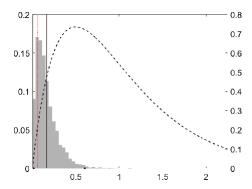
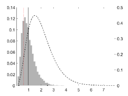
$\beta$	$a\beta/(c-c\beta-\beta b)$

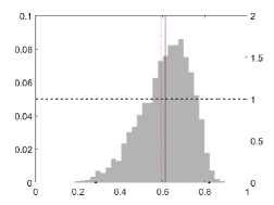
Figure 11: MCMC approximation of the posterior distribution (histogram) of the parameters. In all plots, the estimated value (vertical black solid), the true value (vertical red dotted) and the prior density (dashed).

Low-persistence setting
$\alpha$	$a$
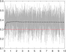
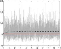
$b$	$c$
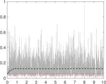
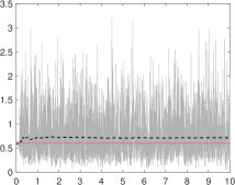
$\beta$	$a\beta/(c-c\beta-\beta b)$

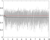
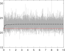
Figure 12: MCMC output for the parameters of the GLK-INAR(1). In all plots, the MCMC draws (gray solid), the progressive MCMC average (dashed black) over the iterations (horizontal axis in thousands), and the true value of the parameter (horizontal red dashed).

Low-persistence setting
$\alpha$	$a$
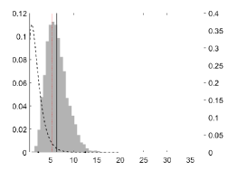
$b$	$c$
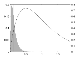
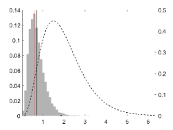
$\beta$	$a\beta/(c-c\beta-\beta b)$

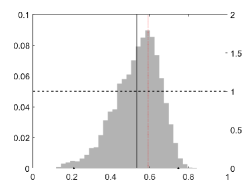
Figure 13: MCMC approximation of the posterior distribution (histogram) of the parameters. In all plots, the estimated value (vertical black solid), the true value (vertical red dotted) and the prior density (dashed).

High-persistence setting
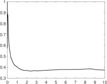
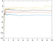
Low-persistence setting

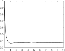
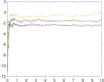
Figure 14: MCMC acceptance rate (left) and adaptive log-scales (right) over the iterations (horizontal axis in thousands).

Appendix C Further real data results

Google search dataset “Climate Change”
$\alpha$	$a$
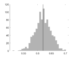
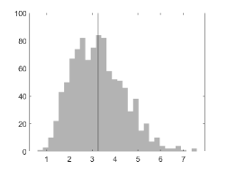
$b$	$c$
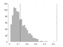
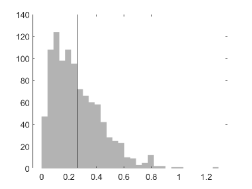
$\beta$	$a\beta/(c-c\beta-\beta b)$

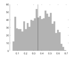
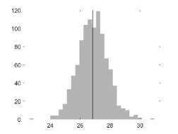
Figure 15: MCMC approximation of the posterior distribution (histogram) of the parameters. In all plots, the estimated value (vertical black solid).

Google search dataset “Global Warming”
$\alpha$	$a$
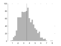
$b$	$c$
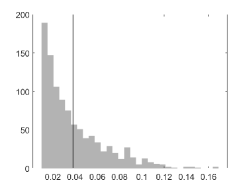
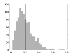
$\beta$	$a\beta/(c-c\beta-\beta b)$

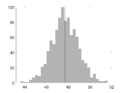
Figure 16: MCMC approximation of the posterior distribution (histogram) of the parameters. In all plots, the estimated value (vertical black solid).

References

- Afrifa-Yamoah and Mueller, (2022) Afrifa-Yamoah, E. and Mueller, U. (2022). Modeling digital camera monitoring count data with intermittent zeros for short-term prediction. Heliyon, 8(1):e08774.
- Aknouche et al., (2021) Aknouche, A., Almohaimeed, B. S., and Dimitrakopoulos, S. (2021). Forecasting transaction counts with integer-valued garch models. Studies in Nonlinear Dynamics & Econometrics, page 20200095.
- Al-Osh and Alzaid, (1987) Al-Osh, M. and Alzaid, A. A. (1987). First-order integer-valued autoregressive (INAR (1)) process. Journal of Time Series Analysis, 8(3):261–275.
- Al-Osh and Aly, (1992) Al-Osh, M. A. and Aly, E.-E. A. (1992). First order autoregressive time series with negative binomial and geometric marginals. Communications in Statistics - Theory and Methods, 21(9):2483–2492.
- Alzaid and Al-Osh, (1993) Alzaid, A. and Al-Osh, M. (1993). Generalized Poisson ARMA processes. Annals of the Institute of Statistical Mathematics, 45(2):223–232.
- Alzaid and Omair, (2014) Alzaid, A. A. and Omair, M. A. (2014). Poisson difference integer valued autoregressive model of order one. Bulletin of the Malaysian Mathematical Sciences Society, 37(2):465–485.
- Anderberg et al., (2021) Anderberg, D., Rainer, H., and Siuda, F. (2021). Quantifying domestic violence in times of crisis: An internet search activity-based measure for the covid-19 pandemic. Journal of the Royal Statistical Society: Series A (Statistics in Society).
- Andersson and Karlis, (2014) Andersson, J. and Karlis, D. (2014). A parametric time series model with covariates for integers in Z. Statistical Modelling, 14(2):135–156.
- Andrieu and Thoms, (2008) Andrieu, C. and Thoms, J. (2008). A tutorial on adaptive MCMC. Statistics and computing, 18(4):343–373.
- Ardia and Bluteau, (2017) Ardia, D. and Bluteau, K. (2017). nse: Computation of numerical standard errors in r. Journal of Open Source Software, 2(10):172.
- Ardia et al., (2018) Ardia, D., Bluteau, K., and Hoogerheide, L. F. (2018). Methods for computing numerical standard errors: Review and application to value-at-risk estimation. Journal of Time Series Econometrics, 10(2).
- Battaglini et al., (2009) Battaglini, A., Barbeau, G., Bindi, M., and Badeck, F.-W. (2009). European winegrowers’ perceptions of climate change impact and options for adaptation. Regional Environmental Change, 9:61–73.
- Berry and West, (2020) Berry, L. R. and West, M. (2020). Bayesian forecasting of many count-valued time series. Journal of Business & Economic Statistics, 38(4):872–887.
- Bourguignon et al., (2016) Bourguignon, M., Vasconcellos, K. L., Reisen, V. A., and Ispány, M. (2016). A Poisson INAR(1) process with a seasonal structure. Journal of Statistical Computation and Simulation, 86(2):373–387.
- Bourguignon and Vasconcellos, (2015) Bourguignon, M. and Vasconcellos, K. L. P. (2015). First order non-negative integer valued autoregressive processes with power series innovations. Brazilian Journal of Probability and Statistics, 29(1):71 – 93.
- Bouzar, (2008) Bouzar, N. (2008). Semi-self-decomposable distributions on . Annals of the Institute of Statistical Mathematics, 60(4):901–917.
- Chen and Lee, (2016) Chen, C. W. and Lee, S. (2016). Generalized Poisson autoregressive models for time series of counts. Computational Statistics & Data Analysis, 99:51–67.
- Chen and Lee, (2017) Chen, C. W. and Lee, S. (2017). Bayesian causality test for integer-valued time series models with applications to climate and crime data. Journal of the Royal Statistical Society: Series C (Applied Statistics), 66(4):797–814.
- Choi and Varian, (2012) Choi, H. and Varian, H. (2012). Predicting the present with Google Trends. Economic Record, 88:2–9.
- Consul and Famoye, (2006) Consul, P. C. and Famoye, F. (2006). Lagrangian probability distributions. Springer.
- Cunha et al., (2018) Cunha, E. T. d., Vasconcellos, K. L., and Bourguignon, M. (2018). A skew integer-valued time-series process with generalized Poisson difference marginal distribution. Journal of Statistical Theory and Practice, 12(4):718–743.
- Drovandi et al., (2016) Drovandi, C. C., Pettitt, A. N., and McCutchan, R. A. (2016). Exact and Approximate Bayesian Inference for Low Integer-Valued Time Series Models with Intractable Likelihoods. Bayesian Analysis, 11(2):325 – 352.
- Eckstein et al., (2021) Eckstein, D., Künzel, V., and Schäfer, L. (2021). Global climate risk index 2021. Who suffers most from extreme weather events? Weather-related loss events in 2019 and 2000-2019. Bonn: Germanwatch.
- Fahad and Wang, (2018) Fahad, S. and Wang, J. (2018). Farmers’ risk perception, vulnerability, and adaptation to climate change in rural pakistan. Land Use Policy, 79:301–309.
- Freeland and McCabe, (2004) Freeland, R. and McCabe, B. P. (2004). Analysis of low count time series data by Poisson autoregression. Journal of Time Series Analysis, 25(5):701–722.
- Freeland, (1998) Freeland, R. K. (1998). Statistical analysis of discrete time series with application to the analysis of workers’ compensation claims data. PhD thesis, University of British Columbia.
- Freeland, (2010) Freeland, R. K. (2010). True integer value time series. AStA Advances in Statistical Analysis, 94(3):217–229.
- Fried et al., (2015) Fried, R., Agueusop, I., Bornkamp, B., Fokianos, K., Fruth, J., and Ickstadt, K. (2015). Retrospective Bayesian outlier detection in INGARCH series. Statistics and Computing, 25(2):365–374.
- Frondel et al., (2017) Frondel, M., Simora, M., and Sommer, S. (2017). Risk perception of climate change: Empirical evidence for Germany. Ecological Economics, 137:173–183.
- (30) Garay, A. M., Medina, F. L., Cabral, C. R., and Lin, T.-I. (2020a). Bayesian analysis of the p-order integer-valued ar process with zero-inflated poisson innovations. Journal of Statistical Computation and Simulation, 90(11):1943–1964.
- (31) Garay, A. M., Medina, F. L., Cabral, C. R. B., and Lin, T.-I. (2020b). Bayesian analysis of the p-order integer-valued ar process with zero-inflated poisson innovations. Journal of Statistical Computation and Simulation, 90(11):1943–1964.
- Geyer, (1992) Geyer, C. J. (1992). Practical Markov chain Monte Carlo. Statistical Science, pages 473–483.
- Guolo and Varin, (2014) Guolo, A. and Varin, C. (2014). Beta regression for time series analysis of bounded data, with application to Canada Google Flu Trends. The Annals of Applied Statistics, 8(1):74 – 88.
- Janardan, (1998) Janardan, K. (1998). Generalized Polya Eggenberger family of distributions and its relation to Lagrangian Katz family. Communications in Statistics-Theory and Methods, 27:2423–2442.
- Janardan, (1999) Janardan, K. (1999). Estimation of parameters of the GPED. Communications in Statistics-Theory and Methods, 28:2167–2179.
- Jin-Guan and Yuan, (1991) Jin-Guan, D. and Yuan, L. (1991). The integer-valued autoregressive (INAR (p)) model. Journal of Time Series Analysis, 12(2):129–142.
- Johnson et al., (2005) Johnson, N. L., Kemp, A. W., and Kotz, S. (2005). Univariate Discrete Distributions, Third Edition. John Wiley & Sons.
- Katz, (1965) Katz, L. (1965). Unified treatment of a broad class of discrete probability distributions. Classical and contagious discrete distributions, 1:175–182.
- Kim and Lee, (2017) Kim, H. and Lee, S. (2017). On first-order integer-valued autoregressive process with Katz family innovations. Journal of Statistical Computation and Simulation, 87(3):546–562.
- Kim and Park, (2008) Kim, H.-Y. and Park, Y. (2008). A non-stationary integer-valued autoregressive model. Statistical Papers, 49(3):485.
- Liesenfeld et al., (2006) Liesenfeld, R., Nolte, I., and Pohlmeier, W. (2006). Modelling financial transaction price movements: A dynamic integer count data model. Empirical Economics, 30(4):795–825.
- Lineman et al., (2015) Lineman, M., Do, Y., Kim, J. Y., and Joo, G.-J. (2015). Talking about climate change and global warming. PloS one, 10(9):e0138996.
- McCabe and Martin, (2005) McCabe, B. and Martin, G. (2005). Bayesian predictions of low count time series. International Journal of Forecasting, 21(2):315–330.
- McCabe and Skeels, (2020) McCabe, B. P. and Skeels, C. L. (2020). Distributions you can count on… but what’s the point? Econometrics, 8(1):9.
- McKenzie, (1985) McKenzie, E. (1985). Some simple models for discrete variate time series. Water Resources Bulletin, 21(4):645–650.
- McKenzie, (1986) McKenzie, E. (1986). Autoregressive moving-average processes with negative-binomial and geometric marginal distributions. Advances in Applied Probability, 18(3):679?705.
- Neal and Subba Rao, (2007) Neal, P. and Subba Rao, T. (2007). MCMC for integer-valued ARMA processes. Journal of Time Series Analysis, 28(1):92–110.
- Pedeli and Karlis, (2011) Pedeli, X. and Karlis, D. (2011). A bivariate INAR(1) process with application. Statistical Modelling, 11(4):325–349.
- Robert and Casella, (2013) Robert, C. and Casella, G. (2013). Monte Carlo statistical methods. Springer Science & Business Media.
- Roberts et al., (1997) Roberts, G. O., Gelman, A., Gilks, W. R., et al. (1997). Weak convergence and optimal scaling of random walk Metropolis algorithms. The Annals of Applied Probability, 7(1):110–120.
- Rydberg and Shephard, (2003) Rydberg, T. H. and Shephard, N. (2003). Dynamics of trade-by-trade price movements: Decomposition and models. Journal of Financial Econometrics, 1(1):2–25.
- Schiavoni et al., (2021) Schiavoni, C., Palm, F., Smeekes, S., and van den Brakel, J. (2021). A dynamic factor model approach to incorporate big data in state space models for official statistics. Journal of the Royal Statistical Society: Series A (Statistics in Society), 184(1):324–353.
- Scott and Varian, (2014) Scott, S. L. and Varian, H. R. (2014). Predicting the present with Bayesian structural time series. International Journal of Mathematical Modelling and Numerical Optimisation, 5(1-2):4–23.
- Scotto et al., (2015) Scotto, M. G., Weiß, C. H., and Gouveia, S. (2015). Thinning-based models in the analysis of integer-valued time series: A review. Statistical Modelling, 15(6):590–618.
- Shahtahmassebi and Moyeed, (2016) Shahtahmassebi, G. and Moyeed, R. (2016). An application of the generalized Poisson difference distribution to the Bayesian modelling of football scores. Statistica Neerlandica, 70(3):260–273.
- Shang and Zhang, (2018) Shang, H. and Zhang, B. (2018). Outliers detection in INAR (1) time series. Journal of Physics: Conference Series, 1053:012094.
- Singh et al., (2017) Singh, R. K., Zander, K. K., Kumar, S., Singh, A., Sheoran, P., Kumar, A., Hussain, S., Riba, T., Rallen, O., Lego, Y., Padung, E., and Garnett, S. T. (2017). Perceptions of climate variability and livelihood adaptations relating to gender and wealth among the adi community of the eastern indian himalayas. Applied Geography, 86:41–52.
- Spiegelhalter et al., (2002) Spiegelhalter, D. J., Best, N. G., Carlin, B. P., and Van Der Linde, A. (2002). Bayesian measures of model complexity and fit. Journal of the Royal Statistical Society: Series B (Statistical Methodology), 64(4):583–639.
- Steutel and van Harn, (1979) Steutel, F. W. and van Harn, K. (1979). Discrete analogues of self-decomposability and stability. The Annals of Probability, pages 893–899.
- Ullah et al., (2018) Ullah, H., Rashid, A., Liu, G., and Hussain, M. (2018). Perceptions of mountainous people on climate change, livelihood practices and climatic shocks: A case study of Swat District, Pakistan. Urban Climate, 26:244–257.
- Weiß, (2008) Weiß, C. H. (2008). Thinning operations for modeling time series of counts-A survey. Advances in Statistical Analysis, 92(3):319.
- Weiß and Kim, (2013) Weiß, C. H. and Kim, H.-Y. (2013). Parameter estimation for binomial AR(1) models with applications in finance and industry. Statistical Papers, 54(3):563–590.
- Yang et al., (2021) Yang, S., Ning, S., and Kou, S. C. (2021). Use internet search data to accurately track state level influenza epidemics. Scientific Reports, 11(1):4023.
- Yi et al., (2021) Yi, D., Ning, S., Chang, C.-J., and Kou, S. C. (2021). Forecasting unemployment using internet search data via prism. Journal of the American Statistical Association, 116(536):1662–1673.
- Yu et al., (2019) Yu, L., Zhao, Y., Tang, L., and Yang, Z. (2019). Online big data-driven oil consumption forecasting with Google trends. International Journal of Forecasting, 35(1):213–223.
- Ziegler, (2017) Ziegler, A. (2017). Political orientation, environmental values, and climate change beliefs and attitudes: An empirical cross country analysis. Energy Economics, 63:144–153.