Optimal loading of hydrogel-based drug-delivery systems

Abstract

Drug-loaded hydrogels provide a means to deliver pharmaceutical agents to specific sites within the body at a controlled rate. The aim of this paper is to understand how controlled drug release can be achieved by tuning the initial distribution of drug molecules in a hydrogel. A mathematical model is presented for a spherical drug-loaded hydrogel. The model captures the nonlinear elasticity of the polymer network and thermodynamics of swelling. By assuming that the drug molecules are dilute, the equations for hydrogel swelling and drug transport partially decouple. A fast optimisation method is developed to accurately compute the optimal initial drug concentration by minimising the error between the numerical drug-release profile and a target profile. By taking the target drug efflux to be piecewise constant, the optimal initial configuration consists of a central drug-loaded core with isolated drug packets near the free boundary of the hydrogel. The optimal initial drug concentration is highly effective at mitigating the burst effect, where a large amount of drug is rapidly released into the environment. The hydrogel stiffness can be used to further tune the rate of drug release. Although stiffer gels lead to less swelling and hence reduce the drug diffusivity, the drug-release kinetics are faster than for soft gels due to the decreased distance that drug molecules must travel to reach the free surface.
Keywords: drug delivery, hydrogels, optimisation, burst effect

1 Introduction

A hydrogel is a two-component system consisting of a deformable polymer network that is saturated with water. The hydrophilic nature of the polymers creates an energetic incentive for water molecules to enter the network via diffusion. In order for the network to accommodate the volume of the water molecules, the polymers must stretch. Imbibition of water therefore continues until the energy cost of elastically deforming the polymer network balances the energy gain of mixing water and polymer. At equilibrium, the volume of a swollen hydrogel can be tens or even thousands of times greater than the volume of the dry polymer network. The ability to precisely control the degree of swelling via stimuli such as temperature, pH, and electric fields has led to hydrogels finding use in a diverse range of applications [1].

Drug-loaded hydrogels have emerged as important systems for the controlled and targetted delivery of pharmaceutical agents [2, 3]. Controlled delivery means that drug molecules are released at a prescribed rate; targetted delivery means that the drug molecules are released at specific locations within the body. The ability to tune the water content and stiffness of hydrogels leads to excellent biocompatibility as they are able to mimic a wide range of biological tissues [4]. In addition, the polymer network provides mechanical and chemical shielding that prevents the degradation of drug molecules before they are released into the body.

Hydrogels provide a pathway to controlled and targetted drug delivery through their tunable, multi-scale architecture and ability to swell when subjected to a stimulus [5]. Hydrogels possess a macroscopic length scale associated with their overall size, which can range from microns to millimetres, and a nanometric length scale associated with the mesh size of the polymer network. Both length scales play key roles in the kinetics of drug release: the gel size controls the distance that drug molecules must travel to reach the gel surface and be released into the environment, whereas the mesh size controls the rate of drug diffusion through the polymer network. If the mesh size is much greater than the hydrodynamic radius of a drug molecule, then drug diffusion is uninhibited by the presence of the polymer network. However, as the mesh size approaches the hydrodynamic radius, drug molecules become increasingly immobilised by the polymer network. Drug molecules that are larger than the mesh size are effectively entrapped by the network and diffusion is completely suppressed. Hydrogel swelling increases the mesh size of the network, thus mobilising drug molecules and initiating their release into the surroundings. By programming a hydrogel to swell in response to specific environmental cues, it is possible to deliver drug payloads to target sites within the body. For example, environmentally responsive hydrogels have been used to target tumours [6] and breast cancer cells [7] by exploiting local increases in pH and temperature relative to healthy tissue.

Due to the increasingly widespread use of hydrogel-based drug-delivery systems, there is a need for broadly applicable methods that can sensitively control drug-release profiles [8]. Although the various length scales in a hydrogel can be harnessed to alter the drug-release kinetics, achieving a desired drug-release profile remains a major challenge. The onset of swelling can drastically change the time scale of drug diffusion by simultaneously increasing the drug diffusivity and the distance that drug molecules must travel to reach the free surface. Moreover, a common problem with drug-delivery systems is the so-called “burst effect”, where a significant proportion of the drug is released in a short initial time frame [9], a phenomenon that can have potentially dangerous effects [10]. While many advances in tunable release kinetics have been made in recent years [11], there is still significant scope for improvement.

The objective of this work is to employ mathematical modelling to explore the potential of tuning the drug-release profile by varying the initial drug concentration in drug-loaded hydrogels. The mathematical model will utilise the theory of nonlinear elasticity to capture the large deformations of the polymer network that occur during swelling and the resulting elastic stresses. The generation of mechanical stress is a particularly important feature to resolve as it enhances the transport of water molecules through the hydrogel via stress-assisted diffusion. An optimisation theory will be developed for computing the initial distribution of drug molecules that leads to the best approximation of a target drug-release profile. The immobility of the drug when the hydrogel is unswollen means that a non-uniform initial concentration can be experimentally achieved in a variety of ways [12] and thus has significant relevance as a control method.

Extensive research on the mathematical modelling of drug-delivery systems has led to a plethora of literature which has been reviewed by Siepmann and Siepmann [13] and Siepmann and Peppas [14]. Caccavo [15] compiled a comprehensive overview of models that have been specifically developed for hydrogel-based drug-delivery systems; these include simple empirical expressions for data fitting, detailed physical models based on continuum mechanics, and statistical and neural-network models. The idea to control the drug-release kinetics via the initial drug concentration was first proposed by Lee [16]. Subsequent developments by Lu et al. [17, 18] involved calculating the optimal initial concentration profile, with drug concentration modelled by the constant-coefficient diffusion equation. Georgiadis and Kostoglou [19] further extended these works to consider the case of a spatially non-uniform diffusion coefficient as well as allowing this diffusion coefficient to be a free variable. However, the models used in these optimisation approaches did not account for the time-dependent swelling of the hydrogel and its subsequent mechanical response.

The key novelty of this paper therefore arises from combining optimisation theory with the use of a fully coupled chemo-mechanical model of a hydrogel based on nonlinear elasticity. Our results reveal that a piecewise-linear drug-release profile is best approximated if the initial drug concentration consists of a central drug-loaded core and a discrete number of drug “packets” near the gel surface, the latter of which are highly localised regions in the gel that are concentrated in drug molecules and which are separated by wide drug-free zones. Moreover, we find that the hydrogel stiffness can be used in tandem with the optimal loading to further tune the drug-release profile and mitigate the burst effect over a wide range of dosage intervals.

The paper is organised as follows. In Sec. 2, we present a model of a drug-loaded hydrogel. In Sec. 3, the equilibrium degree of swelling is computed and its impact on the drug mobility is assessed. We also explore the drug-release profiles for a uniform loading of drug molecules. A theory for the optimal drug loading is developed in Sec. 4 and applied to specific scenarios in Sec. 5. The paper concludes in Sec. 6.

2 Mathematical modelling

We consider the evolution of a spherical, drug-loaded hydrogel after it is placed in an aqueous environment. The drug molecules are assumed to be too large to move through the polymer network when the gel is in its initial, undeformed state. For simplicity, it is assumed that the system remains axisymmetric during swelling and drug release.

Due to the large deformations that occur during swelling, the mechanical response of the hydrogel is described using the framework of nonlinear elasticity. On sufficiently long time scales, the polymers may rearrange to relax the elastic stress, resulting in a viscoelastic material response [20, 21]. Moreover, the polymer network may degrade [22, 23]. Neither of these features will be considered here.

Several thermodynamically consistent hydrogel models based on finite-strain elasticity have been proposed [24, 25, 26]. These models typically assume that the polymer network is swollen by a solute-free liquid and describe the evolution of the mixture towards a state of minimum energy. The addition of a solute, such as drug molecules, can alter the energetic landscape of the system and impact the transport of fluid via cross-diffusion, both of which require extended models to capture [27]. In the context of drug-delivery systems, the volume (or mass) fraction of drug molecules is often small [20]. Consequently, the chemo-mechanics of swelling will not be strongly influenced by the presence of drug molecules [28] and cross-diffusion can be neglected. In formulating the model below, we invoke the assumption that the drug molecules are dilute. As a result, there will be a partial decoupling of the model: governing equations for the hydrogel can be formulated and solved independently from those for the drug. This decoupling will be the key to developing a fast algorithm for optimising the initial drug distribution.

2.1 Bulk equations for the hydrogel

The governing equations for the hydrogel have been derived using thermodynamic arguments by Hennessy et al. [29]; here we specialise the results to a spherical geometry. The equations are formulated in terms of Lagrangian coordinates $\boldsymbol{X}$ associated with the stress-free reference configuration, which is taken to be a dry hydrogel with radius $R_{0}$. The use of Lagrangian coordinates avoids the introduction of a free boundary into the problem. The Lagrangian gradient operator is denoted by $\nabla_{\boldsymbol{X}}$ and is expressed in terms of the usual spherical coordinates. The Eulerian coordinates associated with the current (swollen) configuration are denoted by $\boldsymbol{x}$. For the axisymmetric configurations considered here, we can write $\boldsymbol{X}=R\boldsymbol{e}_{r}$ and $\boldsymbol{x}=r(R,t)\boldsymbol{e}_{r}$, where $R$ and $r$ are Lagrangian and Eulerian radial coordinates, respectively, and $\boldsymbol{e}_{r}$ is the radial basis vector. The deformation gradient tensor $\boldsymbol{\mathsf{F}}=\nabla_{\boldsymbol{X}}\boldsymbol{x}$ describes the local distortion of material elements, whereas its determinant, $J=\det\boldsymbol{\mathsf{F}}$, describes the volumetric changes of material elements. For axisymmetric deformations in spherical geometries, the appropriate form of the deformation gradient tensor is readily calculated as

$$\boldsymbol{\mathsf{F}}=\lambda_{r}\boldsymbol{e}_{r}\otimes\boldsymbol{e}_{r}+\lambda_{\theta}\boldsymbol{e}_{\theta}\otimes\boldsymbol{e}_{\theta}+\lambda_{\varphi}\boldsymbol{e}_{\varphi}\otimes\boldsymbol{e}_{\varphi},$$ (2.1)

where $\boldsymbol{e}_{\theta}$ and $\boldsymbol{e}_{\varphi}$ are the polar and azimuthal basis vectors, $\otimes$ denotes the dyadic product of two vectors, and

$$\lambda_{r}=\frac{\partial r}{\partial R},\quad\lambda_{\theta}=\lambda_{\varphi}=\frac{r}{R},$$ (2.2)

are the principal stretches in the radial, polar, and azimuthal directions. The polymer network and the imbibing fluid, assumed to be water, are treated as incompressible. This assumption, in combination with the limit of a dilute drug, implies that volumetric changes in material elements must be solely associated with the imbibition of water molecules. We therefore impose a molecular incompressibility condition given by

$$J=\lambda_{r}\lambda_{\theta}\lambda_{\varphi}=1+\nu^{w}N^{w},$$ (2.3)

where $\nu^{w}$ and $N^{w}$ are the molecular volume and nominal concentration of water, respectively. Nominal concentrations are expressed in terms of the number of molecules per unit reference (undeformed) volume. The actual concentration of water, i.e. the number of molecules per current (deformed) volume, is defined as $n^{w}=N^{w}/J$. The volume fraction of water $\phi^{w}$ can then be defined as $\phi^{w}=\nu^{w}n^{w}$.

The conservation of water can be expressed as

$$\frac{\partial N^{w}}{\partial t}+\frac{1}{R^{2}}\frac{\partial}{\partial R}\left(R^{2}Q^{w}\right)=0,$$ (2.4)

where $t$ is time and $Q^{w}$ is the nominal diffusive flux given by

$$Q^{w}=-M^{w}\frac{\partial\mu^{w}}{\partial R}.$$ (2.5)

The water mobility $M^{w}$ is defined as

$$M^{w}=\frac{N^{w}}{k_{B}T}\frac{D^{w}(J)}{\lambda_{r}^{2}},$$ (2.6)

with $k_{B}$ denoting Boltzmann’s constant, $T$ the absolute temperature, $D^{w}$ the diffusivity of water in the polymer network, and $\mu^{w}$ the chemical potential of water. The factor of $\lambda_{r}^{-2}$ in (2.6) is a result of mapping Fick’s law in the current configuration to the reference configuration. The water diffusivity is expressed as $D^{w}=D^{w}_{0}J^{a}$, where $a$ is a positive parameter that characterises how strongly the rate of diffusion increases as the polymer network expands. Typically, $a=1.5$; see Bertrand et al. [30].

The chemical potential of water can be expressed as

$$\mu^{w}=\mu^{w}_{0}+\nu^{w}(\Pi^{w}+p),$$ (2.7)

where $\mu^{w}_{0}$ is the chemical potential of a pure bath of water, $\Pi^{w}$ is the osmotic pressure of water, and $p$ is the mechanical pressure. The osmotic pressure captures fluid transport that is driven by concentration gradients and is given by

$$\Pi^{w}=\frac{k_{B}T}{\nu^{w}}\left[\log\left(\frac{\nu^{w}N^{w}}{1+\nu^{w}N^{w}}\right)+\frac{1+\nu^{w}N^{w}+\chi}{(1+\nu^{w}N^{w})^{2}}\right].$$ (2.8)

The Flory parameter $\chi$ describes the strength of energetically unfavourable interactions between polymers and water molecules. Typically, a large value of $\chi$ corresponds to a low degree of swelling, as it becomes energetically costly for fluid and polymers to mix. The dependence of the chemical potential on the mechanical pressure captures transport of fluid down stress gradients and leads to stress-assisted diffusion.

Conservation of linear momentum is given by

$$\frac{1}{R^{2}}\frac{\partial}{\partial R}\left(R^{2}S_{r}\right)-\frac{1}{R}\left(S_{\theta}+S_{\varphi}\right)=0,$$ (2.9a)

$$S_{\theta}-S_{\varphi}=0,$$ (2.9b)

where $S_{i}$ are the principal first Piola–Kirchhoff stresses. The components of the stress can be decomposed into elastic components $\Sigma_{i}$ and a pressure component such that

$$S_{i}=\Sigma_{i}-pJ\lambda_{i}^{-1}.$$ (2.10)

The hydrogel is assumed to be a hyperelastic material described by a neo-Hookean strain energy. Consequently, the elastic components of the stress can be written as

$$\Sigma_{r}=G(\lambda_{r}-\lambda_{r}^{-1}),\quad\Sigma_{\theta}=\Sigma_{\varphi}=G(\lambda_{\theta}-\lambda_{\theta}^{-1}),$$ (2.11)

where $G$ is the shear modulus of the polymer network.

2.2 Bulk equations for drug diffusion

As with the hydrogel model, the equations that govern the transport of drug molecules are written in terms of Lagrangian coordinates. We let $N^{d}$ represent the nominal concentration of drug molecules, which must obey the conservation law

$$\frac{\partial N^{d}}{\partial t}+\frac{1}{R^{2}}\frac{\partial}{\partial R}\left(R^{2}Q^{d}\right)=0.$$ (2.12)

The volume fraction of drug $\phi^{d}$ is defined as $\phi^{d}=\nu^{d}N^{d}/J$, where $\nu^{d}$ is the volume of a drug molecule. The dilute-drug limit requires $\phi^{d}\ll 1$. The diffusive flux of drug molecules, $Q^{d}$, is given by

$$Q^{d}=-\frac{D^{d}(J)}{\lambda_{r}^{2}}\frac{\partial N^{d}}{\partial R}.$$ (2.13)

Various forms of the drug diffusivity $D^{d}$ appear in the literature. A common choice is a Fujita-type expression, in which the drug diffusivity is assumed to exponentially increase with the water concentration. Such forms are suitable for models that neglect the mechanics of the polymer network [31] or which only consider small deformations [21] because the water concentration can serve as a proxy for the degree of swelling that occurs in each material element. Given that our model explicitly captures finite deformations of the polymer network, we choose an expression for the drug diffusivity based on free-volume theory [20]:

$$D^{d}(J)=D^{d}_{\infty}\exp\left[-\frac{\beta}{J-1}\right].$$ (2.14)

The fitting parameter $\beta>0$ controls how strongly the drug diffusivity increases with the volumetric expansion of the polymer network. The value of $D^{d}_{\infty}$ describes the diffusivity of drug molecules when they are uninhibited by the polymer network.

2.3 Boundary and initial conditions

At the centre of the hydrogel, $R=0$, we impose

$$r(0,t)=0,$$ (2.15)

which ensures that the origin in the current state is mapped to the origin in the reference state. In addition, we impose no-flux conditions on the water and drug molecules:

$$Q^{w}(0,t) =0,$$ (2.16a)

$$Q^{d}(0,t) =0.$$ (2.16b)

At the free surface of the hydrogel, $R=R_{0}$, we impose continuity of the chemical potential of water and a stress-free condition, which leads to

$$\mu^{w}(R_{0},t) =\mu^{w}_{0},$$ (2.17a)

$$S_{r}(R_{0},t) =0.$$ (2.17b)

In (2.17), we have set the pressure in the surrounding water to be zero. The surrounding environment is assumed to be a perfect sink for the drug. Therefore, we impose that the concentration of drug at the free surface of the hydrogel is zero:

$$N^{d}(R_{0},t)=0.$$ (2.18)

Consequently, the steady-state configuration will correspond to a swollen, drug-free hydrogel.

Initially, the hydrogel is in a dry state that does not contain water molecules but which is loaded with drug molecules. The initial concentration of drug is denoted by $d$. Therefore, the initial conditions for the model are

$$N^{w}(R,0)=0,\quad N^{d}(R,0)=d(R).$$ (2.19)

Since the hydrogel is initially undeformed, the nominal and actual concentrations coincide at $t=0$. Thus, the initial volume fraction of drug is given by $\phi^{d}(R,0)=\nu^{d}d(R)$. The initial ratio of the total drug volume to the total volume can be defined as

$$\epsilon=\frac{3}{R_{0}^{3}}\int_{0}^{R_{0}}\nu^{d}d(R)R^{2}\,\mathrm{d}R<1.$$ (2.20)

We will impose a value of $\epsilon\ll 1$ to assist in defining the target drug-release profiles. Given that both $\phi^{d}$ and $\epsilon$ represent volume fractions of drug, we will refer to $\phi^{d}$ as the local drug fraction and $\epsilon$ as the global drug fraction.

2.4 Drug efflux and target profiles

The flux of drug molecules out of the hydrogel, hereafter referred to as the efflux, is defined as

$$F(t)=-\frac{\mathrm{d}}{\mathrm{d}t}\left[4\pi\int_{0}^{R_{0}}N^{d}(R,t)R^{2}\,\mathrm{d}R\right]=4\pi R_{0}^{2}Q^{d}(R_{0},t).$$ (2.21)

By integrating the first equality in (2.21) in time and using (2.20), we see that the efflux $F$ must satisfy the condition

$$\int_{0}^{\infty}F(t)\,\mathrm{d}t=\frac{4\pi R_{0}^{3}\epsilon}{3\nu^{d}}.$$ (2.22)

From this point forward, (2.22) will be used in place of (2.20). We now let $A(t)$ denote a target flux profile that is desirable to achieve in practical situations. We will be particularly concerned with piecewise-constant target profiles of the form

$$A(t)=\begin{cases}A_{0},\quad&0\leq t\leq\tau,\\ 0,\quad&\text{otherwise},\end{cases}$$ (2.23a)

where $$\tau A_{0} F A$$ is referred to as the drug-release period and it describes the amount of time needed for all of the drug molecules to be released from the hydrogel. The constant is determined by imposing the constraint in (2.22), which ensures that the actual efflux and the target efflux lead to the same amount of drug being delivered. Therefore, we must have that

$$A_{0}=\frac{4\pi R_{0}^{3}\epsilon}{3\tau\nu^{d}}.$$ (2.23b)

The target profile given by (2.23) has significant physical meaning, as often the goal of drug delivery through hydrogels is to steadily release the drug over a set period of time [32]. The aim of this paper is to determine the initial concentration of drug molecules in the gel that minimises the error between the efflux $F(t)$ and the target profile $A(t)$. The piecewise-constant target profiles in (2.23) provide an excellent means of testing the robustness of our optimisation approach because the discontinunity when $t=\tau$ is difficult to approximate.

2.5 Non-dimensionalisation

The governing equations are written in dimensionless form using the initial gel radius $R_{0}$ as the length scale and $R_{0}^{2}/D^{w}_{0}$ as the time scale. Thus, we write $R=R_{0}\hat{R}$, $r=R_{0}\hat{r}$, and $t=(R_{0}^{2}/D^{w}_{0})\hat{t}$, where hats are used to denote non-dimensional quantities. The chemical potential of water is written as $\mu^{w}=\mu^{w}_{0}+k_{B}T\hat{\mu}^{w}$. The nominal concentrations, the diffusive fluxes, and the drug efflux are written as

$$N^{w}=\frac{1}{\nu^{w}}\,\hat{N}^{w},\quad N^{d}=\frac{\epsilon}{\nu^{d}}\,\hat{N}^{d},\quad Q^{w}=\frac{D^{w}_{0}}{\nu^{w}R_{0}}\hat{Q}^{w},\quad Q^{d}=\frac{\epsilon D^{d}_{\infty}}{\nu^{d}R_{0}}\hat{Q}^{d},\quad F=\frac{\epsilon R_{0}D^{w}_{0}}{\nu^{d}}\hat{F}.$$ (2.24)

The elastic stresses and the pressure are non-dimensionalised according to $\Sigma_{r}=G\hat{E}_{r}$, $\Sigma_{\theta}=G\hat{E}_{\theta}$, and $p=G\hat{p}$. In the dimensionless equations presented below, the hats on the variables will be dropped.

The dimensionless equations for the hydrogel are as follows. The conservation of water reads as

$$\frac{\partial N^{w}}{\partial t} =\frac{1}{R^{2}}\frac{\partial}{\partial R}\left(R^{2}M^{w}\frac{\partial\mu^{w}}{\partial R}\right),$$ (2.25a)

where the water mobility is given by $$M^{w}=N^{w}J^{a}/\lambda_{r}^{2}$$. The chemical potential of water in the gel is given by

$$\mu^{w}=\log\left(\frac{N^{w}}{1+N^{w}}\right)+\frac{1+N^{w}+\chi}{(1+N^{w})^{2}}+\mathcal{G}p,$$ (2.25b)

where $\mathcal{G}=\nu^{w}G/(k_{B}T)$ is a non-dimensional elastic modulus that characterises the energy increase due to elastic deformations relative to the energy decrease of inserting a water molecule into the polymer network. The radial stress balance can be reduced to

$$\frac{\partial\Sigma_{r}}{\partial R}+\frac{2(\Sigma_{r}-\Sigma_{\theta})}{R} =\lambda_{\theta}^{2}\frac{\partial p}{\partial R}.$$ (2.26a)

The elastic components of the stress are written as

$$\Sigma_{r}=\lambda_{r}-\lambda_{r}^{-1},\quad\Sigma_{\theta}=\lambda_{\theta}-\lambda_{\theta}^{-1},$$ (2.26b)

where the non-dimensional expressions for the radial and orthoradial stretches $\lambda_{r}$ and $\lambda_{\theta}$ are identical to those in (2.2). The molecular incompressibility condition can be formulated as

$$J=\lambda_{r}\lambda_{\theta}^{2}=1+N^{w}.$$ (2.27)

Equations (2.25)–(2.27) are solved with the following boundary and initial conditions:

$$r(0,t)=0,\quad\left.\frac{\partial\mu^{w}}{\partial R}\right|_{R=0}=0,\quad\mu^{w}(1,t)=0,\quad S_{r}(1,t)=0,\quad N^{w}(R,0)=0,$$ (2.28)

where the non-dimensional total radial stress $S_{r}$ has the same form as in (2.10).

The diffusion equation that governs the transport of drug molecules through the hydrogel can be written in dimensionless form as

$$\frac{\partial N^{d}}{\partial t} =\frac{\mathcal{D}}{R^{2}}\frac{\partial}{\partial R}\left(R^{2}\frac{D^{d}(J)}{\lambda_{r}^{2}}\frac{\partial N^{d}}{\partial R}\right),$$ (2.29a)

where $$\mathcal{D}=D^{d}_{\infty}/D^{w}_{0}$$. The diffusivity of drug molecules is given by

$$\quad D^{d}=\exp\left(-\frac{\beta}{J-1}\right).$$ (2.29b)

The boundary and initial conditions for the drug concentration are

$$\left.\frac{\partial N^{d}}{\partial R}\right|_{r=0}=0,\quad N^{d}(1,t)=0,\quad N^{d}(R,0)=d(R).$$ (2.29c)

Due to the choice of non-dimensionalisation, the initial volume fraction of drug is given by $\phi^{d}(R,0)=\epsilon d(R)$. The dilute limit therefore requires that $d=O(\epsilon^{-1})$ as $\epsilon\to 0$. The non-dimensional drug efflux is defined as and must satisfy

$$F(t)=-\frac{\mathrm{d}}{\mathrm{d}t}\left(4\pi\int_{0}^{1}N^{d}(R,t)R^{2}\,\mathrm{d}R\right),\qquad\int_{0}^{\infty}F(t)\,\mathrm{d}t=\frac{4}{3}\pi.$$ (2.30)

Similarly, non-dimensionalising the piecewise-constant target profiles in (2.23) leads to

$$A(t)=\begin{cases}\displaystyle 4\pi/(3\tau),\quad&0\leq t\leq\tau,\\ 0,\quad&\text{otherwise}.\end{cases}$$ (2.31)

2.6 Parameter estimation

The initial radius of the hydrogel is assumed to be 2 mm. Gels of this size would likely be surgically implanted into the body or placed directly onto the skin for transdermal drug delivery [5]. Water has a molar volume of $18\cdot 10^{-6}$ m³ mol^-1. Dividing by Avogadro’s number gives a molecular volume of $\nu^{w}=3.0\cdot 10^{-29}$ m³. The shear modulus of the gel, $G$, is taken to be a control parameter. Typical values range from about 10 kPa to 1000 kPa. The Flory interaction parameter $\chi$ depends on the specific type of polymers used to create the gel and is generally a function of composition. However, its value often lies between 0 (for athermal mixtures) and 3. For simplicity, we treat $\chi$ as a constant. Drozdov et al. [26] fitted a similar hydrogel model to experimental data and reported a solvent diffusion coefficient of $D^{w}_{0}\sim 10^{-9}$ m² s^-1. We follow Caccavo et al. [20] and assume that $\beta=1.0$ and that the drug diffusivity $D^{d}_{\infty}$ lies in the range $10^{-12}$ m² s^-1 to $10^{-10}$ m² s^-1. For reference, the diffusivity of paracetamol in water is roughly $6.5\cdot 10^{-10}$ m² s^-1 [33]. The diffusivity of larger macromolecules such as proteins is expected to be substantially smaller. The temperature is fixed at 293 K.

Using these parameter estimates, we find that the non-dimensional shear modulus, $\mathcal{G}$, is between $7\cdot 10^{-5}$ and $7\cdot 10^{-3}$, the smallness of which is characteristic of a soft solid. The diffusivity ratio $\mathcal{D}$ lies between $10^{-3}$ to $10^{-1}$. The time scale of fluid diffusion, $R_{0}^{2}/D^{w}_{0}$, is roughly one hour. Therefore, we assume that the non-dimensional drug-release period $\tau$ appearing in the target flux profile (2.23) ranges from 6 to 24, corresponding to drug release over a 6- to 24-hour window.

2.7 Finite-difference discretisation

The non-dimensional hydrogel model (2.25)–(2.28) is solved using a semi-implicit finite-difference method with a staggered grid. The Lagrangian spatial domain, $0\leq R\leq 1$, is discretised into cells of uniform width. The Eulerian radial coordinate $r$ is solved for on cell edges whereas the pressure $p$ and the nominal fluid fraction $N^{w}$ are solved for on cell midpoints. The conservation equation for the fluid (2.25a) is discretised in time using Euler’s method. All quantities in the dimensionless system (2.25)–(2.28) are treated implicitly, with the exception of the mobility $M^{w}$ in (2.25a), which is treated explicitly. This choice provides greater numerical stability during the first few time steps, where large gradients in the fluid fraction and radial stretch develop. The resulting nonlinear algebraic system is solved using Newton’s method at each time step.

Once the solution to the gel problem is obtained, the linear diffusion problem for the drug (2.29) is solved using an implicit Euler method. The equations are discretised using the same staggered grid for the hydrogel, with the drug concentration $N^{d}$ found on cell midpoints.

3 Benchmarking

The equilibrium states provide valuable information about how swollen the gel becomes for a given set of parameters. From this information, it is possible to assess the change in drug diffusivity that occurs during the swelling process. The equilibrium states correspond to homogeneous gels with swelling ratio $J=J_{\infty}$. The radial and orthoradial stretches are therefore equal and given by $\lambda_{r}=\lambda_{\theta}=J_{\infty}^{1/3}$. The chemical potential of water $\mu^{w}$ and the radial component of the first Piola–Kirchhoff stress $S_{r}$ are both uniform and, from the boundary conditions in (2.28), equal to zero. The latter can be used to obtain an expression for the pressure given by $p=J_{\infty}^{-1/3}-J_{\infty}^{-1}$. Thus, by writing the nominal drug concentration in terms of the swelling ratio $J$ using the incompressibility condition (2.27) and eliminating the pressure in the chemical potential (2.25b), we find that the equilibrium states satisfy

$$\log(1-J_{\infty}^{-1})+J_{\infty}^{-1}+\chi J_{\infty}^{-2}+\mathcal{G}(J_{\infty}^{-1/3}-J_{\infty}^{-1})=0.$$ (3.1)

Once the unique solution for $J_{\infty}$ is obtained from (3.1), the equilibrium drug diffusivity $D^{d}_{\infty}=D^{d}(J_{\infty})$, which represents the maximum value of the drug diffusivity during swelling, can be computed by evaluating (2.29b).

As the Flory interaction parameter $\chi$ increases, there is a marked decrease in the degree of swelling that occurs for all gel stiffnesses; see Fig. 1 (a). Consequently, the equilibrium drug diffusivity decreases as well; see Fig. 1 (b). The curves for the equilibrium swelling ratio and drug diffusivity converge when $\chi>0.7$, indicating that elasticity no longer plays a role in determining the equilibrium. For $\chi<0.7$, the degree of swelling becomes strongly dictated by the gel stiffness $\mathcal{G}$, with softer gels (smaller $\mathcal{G}$) undergoing larger deformations. Correspondingly, the equilibrium drug diffusivity increases with decreasing $\mathcal{G}$ as well. For the softest gels ($\mathcal{G}=7\cdot 10^{-5}$), the drug diffusivity $D^{d}$ approaches unity, implying that drug diffusion becomes uninhibited by the presence of the polymer network.

The increase in drug diffusivity due swelling is counteracted by the increase in distance that drug molecules must travel to reach the free surface. This increase in distance is captured by the factor of $\lambda_{r}^{-2}$ in (2.29a), which is equal to $J_{\infty}^{-2/3}$ at equilibrium. We can thus define the equilibrium drug mobility as $D^{d}(J_{\infty})J_{\infty}^{-2/3}$ to capture the competing effects of increases in diffusivity and gel size. For $0<\chi<0.7$, the equilibrium mobility increases with the gel stiffness, as seen in Fig. 1 (c). Thus, stiffer gels are, in fact, more effective at releasing drug molecules because the reduction in gel size completely offsets the smaller drug diffusivity. The strong dependence of the drug mobility on the gel size underscores the importance of capturing finite deformations in the model.

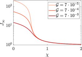
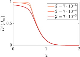
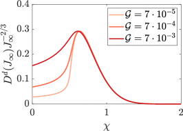
Figure 1: Equilibrium values of the (a) swelling ratio $J_{\infty}$, (b) drug diffusivity $D^{d}(J_{\infty})$, and (c) drug mobility $D^{d}(J_{\infty})J_{\infty}^{-2/3}$, plotted as functions of the Flory interaction parameter $\chi$ for different non-dimensional gel stiffnesses $\mathcal{G}$. The diffusivity $D^{d}$ is given by (2.29b).

We explore the baseline drug-release dynamics for various gel stiffnesses by assuming that the initial loading of the drug is uniform; that is, we take $d(R)\equiv 1$. The Flory parameter is set to $\chi=0.5$ in order to capture changes in the equilibrium state with gel stiffness. By numerically solving the governing equations, we compute the drug efflux $F(t)$ according to (2.21) and the fractional drug release defined as

$$\mathcal{R}(t)=1-\frac{\mathcal{M}(t)}{\mathcal{M}(0)},\quad\mathcal{M}(t)=4\pi\int_{0}^{1}N^{d}(R,t)R^{2}\,\mathrm{d}R.$$ (3.2)

The numerical results are shown in Fig. 2, where, for reference, we also plot a target profile in which the drug efflux is constant over a 24-hour period, corresponding to a piecewise-linear fractional drug release. We consistently observe a large initial “burst” where the drug efflux is large, resulting in a rapid release of drug from the gel. In particular, half of the drug molecules are released within the first four hours. The softest gels have the slowest drug-release kinetics, as expected from the equilibrium drug mobility seen in Fig. 1 (c), and thus provide the closest approximation to the target profile.

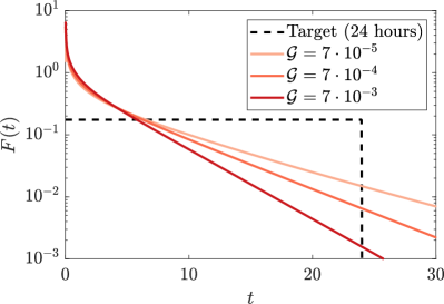
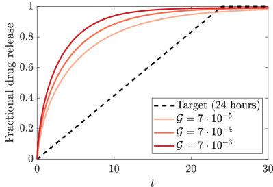
Figure 2: Drug-release dynamics with a uniform initial loading of drug molecules, $d(R)\equiv 1$. (a) The efflux of drug molecules. (b) The fractional amount of drug released into the environment. The parameter values are $\chi=0.5$ and $\mathcal{D}=0.1$.

4 Theory of optimal drug loading

The bursting observed in Fig. 2 is a generic phenomenon that occurs for all parameter values. Achieving a uniform efflux, or a linear drug-release profile, simply by parameter variation is not possible. Therefore, we explore how the initial drug concentration $d(R)$ can be varied to bring the efflux $F(t)$ as close as possible to a prescribed target profile $A(t)$.

4.1 Problem definition

The objective function that measures the difference between $F(t)$ and $A(t)$ is taken to be

$$H(d):=\int_{0}^{\infty}(F(t)-A(t))^{2}\,\mathrm{d}t,$$ (4.1)

which penalises sustained deviations from the target profile; short periods of time where the drug release is different from the desired profile are unimportant. A similar objective function was used by Lu et al. [17], but here we ignore the cost of the drug, which is constant for a fixed value of $\epsilon$, corresponding to a fixed amount of drug. While (4.1) is a good measure of the “closeness” of $F(t)$ and $A(t)$, it is also important to impose that the total drug delivered is the same as the target total amount. This means

$$\int_{0}^{\infty}F(t)\,\mathrm{d}t=\int_{0}^{\infty}A(t)\,\mathrm{d}t=\frac{4}{3}\pi.$$ (4.2)

The only other constraint on the function $d(R)$ is that

$$d(R)\geq 0,\quad\forall R\in(0,1).$$ (4.3)

The endpoint value $d(1)=0$, which is necessary for the boundary conditions, can be ignored as it contributes zero volume of drug to the system. For the moment, we will consider an infinitely dilute drug with $\epsilon\to 0$ and thus will not impose an upper bound on $d$. Thus, the aim is to minimise (4.1) subject to (4.2) and (4.3).

4.2 Impossibility of a perfect solution

It may seem that there is enough freedom in choosing $d(R)$ to ensure that $F(t)\equiv A(t)$ for each possible choice of target profile $A$. However, the long-time behaviour of drug release means that this is not the case. Recall that, at long times, the hydrogel expands to a uniform equilibrium, as discussed in Sec. 3. Thus, by assuming the convergence to the equilibrium state is uniform, then, to leading order, the diffusion equation for the drug becomes

$$\frac{\partial N^{d}}{\partial t}\sim\frac{\mathcal{D}D^{d}(J_{\infty})J_{\infty}^{-2/3}}{R^{2}}\frac{\partial}{\partial R}\left(R^{2}\frac{\partial N^{d}}{\partial R}\right)\text{ as }t\to\infty.$$ (4.4)

By seeking a separable solution, it is straightforward to show that the leading behaviour in time of the efflux is given by

$$F(t)=-\frac{\mathrm{d}}{\mathrm{d}t}\left(4\pi\int_{0}^{1}R^{2}N^{d}(R,t)\,\mathrm{d}R\right)=O\left(\exp\left(-\mathcal{D}D^{d}(J_{\infty})J_{\infty}^{-2/3}\pi t\right)\right)\text{ as }t\to\infty.$$ (4.5)

Thus, if the target profile $A(t)$ has slower-than-exponential decay, for example, then it is impossible that $F(t)=A(t)$ everywhere, so any optimal solution will have a non-zero value of $H$.

4.3 Formulation of a discrete optimsation problem

The linearity of the drug-diffusion problem (2.29) can be exploited to derive a discrete optimisation problem that approximates the full problem given by (4.1)–(4.3). First suppose $\{N_{i}^{d}(R,t)\}_{i}$ is a set of $M$ functions satisfying (2.29a) and its boundary conditions (2.29c), with initial conditions $\{\xi_{i}(R)\}_{i}$. Moreover, let $\{f_{i}(t)\}_{i}$ be the corresponding drug effluxes. Suppose further that $d_{i}$ are real constants. Then, by defining the initial drug concentration as

$$d(R) =\sum_{i=1}^{M}d_{i}\xi_{i}(R),$$ (4.6a)

the solution for the drug concentration $$N^{d} F$$ and the drug efflux can be written as

$$N^{d}(R,t)=\sum_{i=1}^{M}d_{i}N^{d}_{i}(R,t),\quad F(t)=\sum_{i=1}^{M}d_{i}f_{i}(t).$$ (4.6b)

In light of (4.6b), we refer to each $f_{i}$ as a partial efflux. The initial drug concentration $d(R)$ in (4.6a) is now written as a sum of spherical delta functions that are centred at $M$ distinct radial coordinates $0<R_{i}<1$ by defining

$$\xi_{i}(R)=\frac{\delta(R-R_{i})}{4\pi R^{2}}.$$ (4.7)

Each weight $d_{i}$ in (4.6a) therefore corresponds to the number of drug molecules located at the point $R_{i}$. The discrete optimisation problem will compute the optimal values for the $M$ weights $d_{1}$, $d_{2}$, $\ldots$, $d_{M}$. Since $f_{i}(t)$ denotes the drug efflux that is obtained from using $\xi_{i}$ as an initial condition, we have that

$$\int_{0}^{\infty}f_{i}(t)\,\mathrm{d}t=4\pi\int_{0}^{1}\xi_{i}(R)R^{2}\,\mathrm{d}R=1,$$ (4.8)

which implies that

$$\int_{0}^{\infty}F(t)\,\mathrm{d}t=\sum_{i=1}^{M}d_{i}\int_{0}^{\infty}f_{i}(t)\,\mathrm{d}t=\sum_{i=1}^{M}d_{i}.$$ (4.9)

By collecting the weights $d_{i}$ into a vector $\mathbf{d}=(d_{1},d_{2},\ldots,d_{M})$, we can formulate the following discrete optimisation problem:

$$\text{min}\left\{H(\textbf{d}):\textbf{d}\geq\textbf{0}\text{ , }\sum_{i=1}^{M}d_{i}=\int_{0}^{\infty}A(t)\,\mathrm{d}t\right\},$$ (4.10)

where the objective function $H$ is now

$$H(\textbf{d})=\int_{0}^{\infty}\left(\sum_{i=1}^{M}d_{i}f_{i}(t)-A(t)\right)^{2}\,\mathrm{d}t,$$ (4.11)

which is a quadratic function of the variables $d_{i}$. To practically calculate the integral in (4.11), it is necessary to restrict the domain of integration to $[0,T]$ for some large $T$; we find that $T=50$ is a sensible choice.

4.4 Convexity of the objective function

A useful property of the objective function $H$ given by (4.11) is that it is a convex, quadratic function of d. This can be seen by expanding the integrand to give

$$H(\textbf{d})=\sum_{i=1}^{M}\sum_{j=1}^{M}\left(d_{i}d_{j}\int_{0}^{\infty}f_{i}(t)f_{j}(t)\,\mathrm{d}t\right)-2\sum_{i=1}^{M}\left(d_{i}\int_{0}^{\infty}A(t)f_{i}(t)\,\mathrm{d}t\right)+\int_{0}^{\infty}A(t)^{2}\,\mathrm{d}t,$$ (4.12)

which can be concisely written as

$$H(\textbf{d})=\frac{1}{2}\textbf{d}^{T}\boldsymbol{S}\textbf{d}-\textbf{d}^{T}\textbf{q}+\int_{0}^{\infty}A(t)^{2}\,\mathrm{d}t,$$ (4.13)

where $\boldsymbol{S}\in\mathbb{R}^{M\times M}$ and $\textbf{q}\in\mathbb{R}^{M}$ are defined by

$$S_{ij}=2\int_{0}^{\infty}f_{i}(t)f_{j}(t)\,\mathrm{d}t,\qquad q_{i}=2\int_{0}^{\infty}A(t)f_{i}(t)\,\mathrm{d}t.$$ (4.14)

In particular, $\boldsymbol{S}$ is positive semi-definite as, for any $\mathbf{v}\in\mathbb{R}^{M}$,

$$\mathbf{v}^{T}\boldsymbol{S}\mathbf{v} =2\int_{0}^{\infty}\sum_{i=1}^{M}\sum_{j=1}^{M}\left(v_{i}f_{i}(t)f_{j}(t)v_{j}\right)\,\mathrm{d}t=2\int_{0}^{\infty}\left(\sum_{i=1}^{M}v_{i}f_{i}(t)\right)^{2}\,\mathrm{d}t\geq 0.$$ (4.15)

Therefore, $H$ is convex as $\boldsymbol{S}$ is the Hessian matrix of $H$. Using standard convex programming results [34], we can prove that a constrained global minimum exists and that constrained local and global minima are equivalent; details of the proofs are provided in Appendix A. Thus, the global minimum can be calculated by simply finding a local minimum. For the remainder of this paper, the optimal value of $H$ will be denoted as $H^{*}$.

4.5 Numerical implementation

The discrete optimisation problem (4.10)–(4.11) is numerically solved by discretising the governing equations using the finite-difference method described in Sec. 2.7. In particular, the radial domain is discretised into $M$ cells of width $\Delta R=1/M$. The radial coordinates $R_{i}$ used to formulate the discrete optimisation problem (see (4.7)) are chosen to coincide with the positions of the $M$ cell midpoints. The domain of each cell can then be defined as $\Omega_{i}=\{R:R_{i}^{-}<R<R_{i}^{+}\}$ where $R_{i}^{\pm}=R_{i}\pm\Delta R/2$ represent the cell edges. The spherical delta functions given by (4.7) are replaced with step functions defined by

$$\xi_{i}(R)=\begin{cases}\frac{3}{4\pi}\left[(R_{i}^{+})^{3}-(R_{i}^{-})^{3}\right]^{-1},&\quad R\in\Omega_{i},\\ 0,&\quad\text{otherwise},\end{cases}$$ (4.16)

where $i=1,2,\ldots,M$. The functions $\xi_{i}$ in (4.16) can be interpreted as localised packets of drug located at the $i$-th cell.

For a given set of parameter values, we first numerically solve the dimensionless hydrogel equations. We then numerically solve the drug-diffusion problem using each initial condition $\xi_{i}$ in (4.16) to compute the drug concentration $N^{d}_{i}$ and the partial efflux $f_{i}$. The set of partial effluxes $\{f_{i}\}_{i}$ is then used in the discrete optimisation problem (4.10)–(4.11), which is solved using MATLAB’s quadratic programming algorithm quadprog. The analytical results developed in Sec. 4.4 and Appendix A ensure that quadprog will rapidly converge to a global minimum. The ability to pre-compute the partial effluxes, which requires one solution to the nonlinear hydrogel model and $M$ solutions of the linear drug-diffusion model, results in a highly efficient scheme for the numerical optimisation. After determining the optimal weights $d_{i}$, the total efflux $F$ and the drug concentration $N^{d}$ can be constructed using (4.6b).

4.6 The partial effluxes from localised drug loadings

The partial effluxes $f_{i}(t)$ obtained from the localised drug packets given by (4.16) act as basis functions in the construction of the total efflux $F(t)$, as seen in (4.6b). Therefore, the key to understanding the optimal solution lies in the time evolution of the partial effluxes $f_{i}(t)$. If a drug packet is placed sufficiently close to the free boundary of the gel, then the correponding efflux $f_{i}$ monotonically decreases from a large initial value; see Fig. 3. In this case, the large initial efflux is driven by the incompatibility between the initial condition and the perfect sink boundary condition, the latter of which forces the drug concentration to rapidly tend to zero. If a drug packet is placed in the bulk of the gel, then the efflux first increases from zero to a peak value, after which it exponentially decays. The transient increase in efflux is driven by the increase in drug mobility that occurs due to swelling. As placement of the drugs moves further from the outer boundary, the longer it takes for the efflux to reach its peak value, as can be seen from Fig. 3. Eventually, all of the effluxes $f_{i}$ exponentially decay with the same rate, highlighting the unavoidable long-term behaviour of the drug efflux discussed in Sec. 4.2.

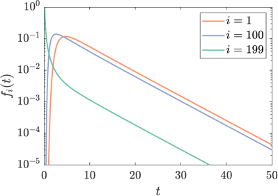
Figure 3: Plots of the partial drug effluxes $f_{i}(t)$ for $i=1$, $i=100$, and $i=199$ due to the packet-like initial concentrations (4.16). The values of $i$ correspond to $R=0$, $R=0.5$ and $R=1$, respectively. The parameter values are $\chi=0.5$, $\mathcal{D}=0.1$, and $\mathcal{G}=7\cdot 10^{-4}$. The numerical simulations are based on using $M=199$ cells.

From the observations made from Fig. 3, it follows that the drug concentration close to the boundary can be utilised to capture the target profile $A(t)$ at small times. The drug concentration in the bulk of the gel enables the target profile to be captured at intermediate times. Capturing the target profile after all of the effluxes $f_{i}$ have peaked is particularly difficult and requires amplifying the drug concentration near the gel centre at the expense of potential overshoots at intermediate times.

5 Case studies

We apply our theory of optimal drug loading to specific scenarios by considering non-dimensional piecewise-constant target profiles with the same form as (2.31).

5.1 Optimal solutions for a 12-hour drug-release period

As a generic example, consider the optimal solution when $\tau=12$, corresponding to a constant release of drug over a 12-hour period. The parameter values are set to $\chi=0.5$, $\mathcal{G}=7\cdot 10^{-4}$, and $\mathcal{D}=0.1$, which are the same as those used when computing the partial effluxes $f_{i}(t)$ in Fig. 3.

The optimal initial drug distribution is formed of distinct, concentrated packets that are separated by large drug-free regions; see Fig. 4 (a). The concentration in the packets decreases as their distance from the gel centre increases. Such a distribution is expected on physical grounds. Small concentrations of drug near the free boundary offset the initial largeness of the corresponding partial effluxes seen in Fig. 3. The drug in the central packet at $R=0$ sustains the long-term drug efflux. However, to reach the free surface, the drug molecules in the central packet much diffusively spread across the entire gel, resulting in a diminished concentration gradient and hence diffusive flux. The largeness of the concentration in the central packet offsets this behaviour.

The corresponding optimal drug efflux $F(t)$ consists of a sequence of pulses of increasing amplitude; see Fig. 4 (b). Each pulse is associated with one of the packets in the initial drug concentration. The small quantity of drug in the packet near $R=1$ is responsible for the first pulse, which provides an approximation of the target profile $A(t)$ for small times. Then, as the pulse from this packet of drug diminishes, the pulse from the next packet begins, counteracting this decrease. This pattern continues until the drug in the central packet nearest $R=0$ is released to create the largest pulse, which then exponentially decays. Due to the exponential tail, the optimal efflux overshoots the target profile after the discontinuity at $t=12$. The overshoot is compensated by a substantial undershoot beforehand when $7<t<12$. The undershoot is itself compensated by an overshoot when $4<t<7$, and the sequence repeats until $t=0$.

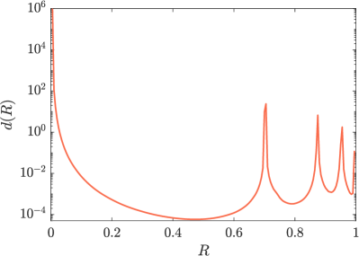
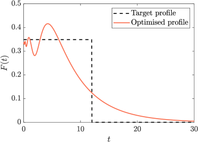
Figure 4: The optimal (a) initial drug concentration $d(R)$ and (b) corresponding drug efflux $F(t)$. The dashed line represents the piecewise-constant target profile. The parameter values are $\chi=0.5$, $\mathcal{D}=0.1$, $\mathcal{G}=7\cdot 10^{-4}$, and $\tau=12$.

The gel stiffness $\mathcal{G}$ plays an important role in the optimal solution by modulating the equilibrium drug mobility $D^{d}(J_{\infty})J_{\infty}^{-2/3}$ and hence the decay rate of the efflux $F(t)$. When $\chi=0.5$, the mobility increases with the gel stiffness; see Fig. 1 (c). For stiff gels with $\mathcal{G}=7\cdot 10^{-3}$, the faster decay rate leads to less overshoot after the discontinuity in the target profile, but results in much larger undershoots and overshoots beforehand; see Fig. 5 (a). For soft gels with $G=7\cdot 10^{-5}$, the slower decay rate leads to a greater overshoot after the discontinuity, which is compensated by an efflux that is consistently below the target profile beforehand.

By computing the fractional drug release using (3.2), we find that the gel stiffness can be combined with the optimal loading to tune the drug-release profile and, in particular, eliminate the burst effect. For an intermediate stiffness of $\mathcal{G}=7\cdot 10^{-4}$, the target drug-release profile is perfectly captured during the first 7.5 hours, as shown in Fig. 5 (b), despite the sequence of undershoots and overshoots that occur in the efflux. However, after 7.5 hours, there is a sharp decrease in the release rate, resulting in a marked departure from the target profile and a prolongation of the drug-release period. In particular, 19 hours are needed for 95% of the drug to be released. By increasing the gel stiffness to $\mathcal{G}=7\cdot 10^{-3}$, the release rate can be accelerated, which leads to a temporary overshoot compared to the target release profile but lessens the long-term undershoot; in this case, only 14 hours are required for 95% of the drug to be released. Decreasing the stiffness to $\mathcal{G}=7\cdot 10^{-5}$ leads to a slower drug-release profile that is consistently below the target curve.

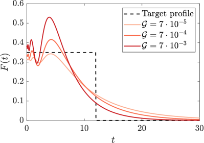
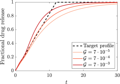
Figure 5: A comparison of optimal and target (a) effluxes and (b) fractional drug-release profiles for different gel stiffnesses $\mathcal{G}$ in the case of $\chi=0.5$, $\mathcal{D}=0.1$, and $\tau=12$.

5.2 Tuning the drug-release profile

Motivated by the results in Fig. 5, we now explore how the gel stiffness can be used to further optimise the drug-release profile. More specifically, we compute the optimal value of the objective function $H$, denoted by $H^{*}$, across a range of gel stiffnesses $\mathcal{G}$ and different combinations of the drug diffusivity $\mathcal{D}$ and drug-release period $\tau$.

We first consider the case when $\mathcal{D}=0.1$. For a 12-hour drug-release period with $\tau=12$, the curve of $H^{*}$ as a function of $\mathcal{G}$ has a global, internal minimum at $\mathcal{G}=7\cdot 10^{-4}$; see Fig. 6 (a). Thus, the target profile is best approximated when the gel stiffness is $7\cdot 10^{-4}$, in agreement with the results in Fig. 5. Hydrogels that are stiffer or softer would increase or decrease the equilibrium drug mobility, respectively, and hence lead to drug molecules that are released too quickly or slowly to be optimal. The increase in drug-release rate that occurs for stiffer hydrogels can be advantageous for capturing target profiles with smaller drug-release periods. Conversely, softer hydrogels, with their slower drug-release kinetics, will be better suited for capturing target profiles with larger drug-release periods. Indeed, when the drug-release period $\tau$ is decreased to 6 hours, the objective function $H^{*}$ monotonically decreases with $\mathcal{G}$; when $\tau$ is increased to 18 or 24 hours, the objective function monotonically increases with $\mathcal{G}$.

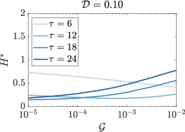
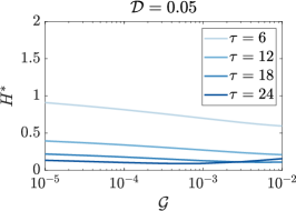
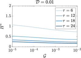
Figure 6: The variation in the optimal value of the objective function $H^{*}$ with the gel stiffness $\mathcal{G}$ for different drug-release periods $\tau$ and non-dimensional drug diffusivities $\mathcal{D}$. Here, we take $\chi=0.5$.

Decreasing the drug diffusivity via the dimensionless parameter $\mathcal{D}$ leads to stiffer gels performing better, as seen in Fig. 6 (b)–(c). In this case, the reduction in swelling and the smaller radial extent of the hydrogel makes up for the decrease in the rate of drug diffusion. As a final remark, the model can be simplified for small values of $\mathcal{D}$ by rescaling time as $t=\mathcal{D}^{-1}t^{\prime}$ and then taking the limit $\mathcal{D}\to 0$. The resulting quasi-static model describes linear drug diffusion throughout a uniformly swollen hydrogel that is in chemo-mechanical equilibrium with the surrounding environment.

5.3 Optimal solution with finite drug diluteness

The numerical results in Sec. 5.1–5.2 are based on the assumption of an infinitely dilute drug, as characterised by the limit $\epsilon\to 0$. However, in practice, the drug molecules can account for roughly 10% ($\epsilon=0.1$) of the total initial volume [31]. Thus, when computing the optimum initial volume fraction of drug, $\phi^{d}(R,0)=\epsilon d(R)$, using the solution for $d$ shown in Fig. 4 (a), we see that it exceeds one. This unphysical result stems from not imposing upper bounds on the initial drug concentration when working in the infinitely dilute limit.

We now consider situations where the drug molecules have a finite diluteness. Thus, the global drug fraction $\epsilon$ is taken to be a small but finite number. We assume that the initial volume fraction of drug fraction satisfies $0<\phi^{d}(R,0)<0.2$, which implies that $0<d(R)<0.2\epsilon^{-1}$. The optimisation theory developed in Sec. 4 still applies because the upper bound on $d(R)$ translates into upper bounds on each $d_{i}$ in the discrete optimsation problem, which are straightforward to accommodate; see Appendix A for full details. Thus, the newly constrained discrete optimisation problem admits global minima that can be readily computed using Matlab’s quadprog function.

As the global drug fraction $\epsilon$ is increased from zero, the optimal initial drug concentration $d(R)$ is found to retain a structure that consists of several drug-loaded packets near the free boundary of the gel; see Fig. 7 (a). However, the central packet near $R=0$ that was observed in the infinitely dilute case ($\epsilon\to 0$) has been replaced with a uniformly loaded core in which the local drug fraction takes on its maximum value. The radial extent of the drug-loaded core increases with the global drug fraction $\epsilon$. To explain these results, we recall that the initial drug concentration becomes increasingly constrained as $\epsilon$ increases from zero. Thus, if the initial drug concentration for the infinitely dilute case has any packets that exceed the maximum allowable concentration, then the drug molecules in these packets are simply distributed over a greater volume, that is, a over greater radial extent. Any packets that have concentrations below the maximum are mostly unaffected by the constraint, although their position might shift slightly. From the optimal initial drug concentrations, we can conclude that when increasing the total drug load for a fixed drug-release period $\tau$, it is advantageous to preferentially place drug molecules at the centre of the hydrogel.

The similarities in the optimal initial drug profiles lead to optimal drug effluxes $F(t)$ that still consist of pulse sequences that overshoot and undershoot the target profile, as shown in Fig. 7 (b). However, due to the increase in the radial extent of the drug-loaded core that occurs as $\epsilon$ increases, the penultimate overshoot in the efflux, characterised by that which leads to its maximum value, has a greater amplitude and occurs sooner in the drug-release process. Consequently, the drug-release kinetics will be more prone to bursting when additional drug molecules are loaded into the hydrogel and the drug-release period is held constant.

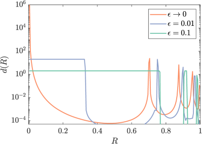
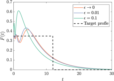
Figure 7: Optimal (a) initial drug concentrations $d(R)$ and (b) effluxes $F(t)$ for different maximal drug dilutions, as measured through the global drug fraction $\epsilon$ defined by (2.20). The parameter values are $\chi=0.5$, $\mathcal{G}=7\cdot 10^{-4}$, $\mathcal{D}=0.1$.

When considering finite values of the global drug fraction $\epsilon$, the hydrogel stiffness $\mathcal{G}$ can still be used to further tune the drug-release profile. Specifically, stiffer and softer gels accelerate and decelerate the release of drug molecules, respectively; see Fig. 8. However, compared to the case of an infinitely dilute drug, as shown in Fig. 5 (b) for the same parameter set, we clearly see that a finite value of $\epsilon$ generally leads to a more rapid release of drug, particularly at small times. Thus, even the optimal drug-release profiles exhibit stronger burst-like characteristics when more drug is loaded into the hydrogel. Tuning the hydrogel stiffness may be an effective means of further mitigating the burst effect in real-world applications, where the initial drug volume is indeed finite, and overcome limitations with simply optimising over the initial distribution of drug molecules.

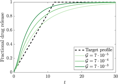
Figure 8: Optimised fractional drug-release profiles when the initial global drug fraction is fixed at $\epsilon=0.1$. The other parameter values are $\chi=0.5$ and $\mathcal{D}=0.1$.

6 Conclusion

The goal of this paper is to explore the possibility of optimising the drug-release profile in hydrogel-based drug-delivery systems by tuning the initial drug distribution. Thus, a model of a spherical drug-loaded hydrogel that captures large elastic deformations due to swelling is presented. By considering the limit of a dilute drug, the equations for the hydrogel decouple from the equations for drug transport, the latter of which become linear in the drug concentration. Using this model, a theory for optimising the drug-release profile via the initial drug concentration is developed. The dilute-drug assumption paves the way towards a fast numerical solver for the optimisation problem by enabling the partial drug effluxes $f_{i}(t)$ used as basis functions to be pre-computed.

For target drug effluxes that are piecewise-constant functions, the optimal initial distribution of drug molecules generally consists of a central drug-loaded packet or core with several isolated packets near the hydrogel boundary. The radial extent of the central core increases with the amount of drug that is loaded into the hydrogel. Numerical simulations reveal that the optimal initial drug concentrations are highly effective at mitigating the burst effect and limiting the initial release of drug into the surroundings. Moreover, the corresponding drug-release profiles provide reasonable approximations to the target profiles for all times.

The hydrogel stiffness provides an additional parameter that can be used to tune the drug-release profile. However, the stiffness plays a non-trivial role in the drug-release kinetics because it affects both the drug diffusivity and the distance that drug molecules must travel to reach the free surface. Softer hydrogels undergo a greater degree of swelling; as a result, the drug diffusivity increases but so does the distance to the free surface. For the parameter range considered here, we find that the rate of drug release is more strongly affected by variations in the radial extent of the hydrogel than variations in the drug diffusivity. Consequently, softer hydrogels lead to slower drug-release kinetics and are better suited for applications that require the administration of drugs over long periods of time. Moreover, the strong dependence of drug transport on the size of the hydrogel highlights the importance of capturing finite deformations in the model.

The results presented here generate new questions about the impact of viscoelasticity and network degradation on the optimal loading of hydrogels. A reduction in the elastic stress due to viscous rearrangement of the polymers could trigger additional swelling and hence slow the release of drug molecules. Bulk degradation of the hydrogel, which could be captured by a decreasing gel stiffness in time, could have similar consequences. By working within the dilute-drug limit, fast numerical methods can be developed to optimise drug-release profiles calculated from extended models. A detailed study of the non-dilute limit would also be insightful by capturing how the transport of drug molecules is affected by the mechanical response of the hydrogel. Mathematical modelling will play a key role in understanding these points and thus lead to finer control over the delivery of drug payloads using hydrogel carriers.

Appendix A Existence and globality of local minima

In this appendix we prove that global minima exist and that local minima are equivalent to global minima. To do so, it is helpful to recall that a definition of convexity (for twice continuously differentiable functions) is that $\forall\mathbf{v}$, $\mathbf{w}\in\mathbb{R}^{M}$ and $\alpha\in[0,1]$,

$$\alpha H(\mathbf{v})+(1-\alpha)H(\textbf{w})-H(\alpha\mathbf{v}+(1-\alpha)\mathbf{w})\geq 0.$$ (A.1)

We now consider the discrete optimisation problem given by (4.10)–(4.11). The feasible set for d is bounded as $\textbf{d}\geq\textbf{0}$ and

$$d_{i}=\int_{0}^{\infty}d_{i}f_{i}(t)\,\mathrm{d}t\leq\int_{0}^{\infty}F(t)\,\mathrm{d}t=\int_{0}^{\infty}A(t)\,\mathrm{d}t<\infty.$$ (A.2)

Moreover, the feasible set is non-empty as all constraints are satisfied by, for example,

$$d_{1}=\int_{0}^{\infty}A(t)\,\mathrm{d}t,\quad d_{2},d_{3},\ldots,d_{M}=0.$$ (A.3)

Since $H(\textbf{d})$ is continuous, the Boundedness Theorem shows that $H$ has a global minimum in this feasible set.

Using standard convex programming results [34], we can prove that constrained local and global minima are equivalent. To do so, we consider a more general convex programming problem given by

$$\min\left\{H(\textbf{d}):\textbf{L}\textbf{d}\leq\textbf{b}\right\},$$ (A.4)

where L is a matrix and b a vector such that $S:=\{\textbf{d}:\textbf{L}\textbf{d}\leq\textbf{b}\}\neq\emptyset$. Note that the constraint $\textbf{L}\textbf{d}\leq\textbf{b}$ can account for upper bounds on each $d_{i}$. In this constrained optimisation problem, local minima can be defined by first considering the set of “feasible directions” $V(\textbf{d}^{*})$ at a point $\textbf{d}^{*}\in S$. This is given by

$$V(\textbf{d}^{*})=\left\{\boldsymbol{v}:\exists\beta>0\quad\text{such that}\quad\textbf{d}^{*}+\gamma\boldsymbol{v}\in S\quad\forall\gamma\in[0,\beta]\right\}.$$ (A.5)

The vectors $\mathbf{v}\in V(\mathbf{d}^{*})$ are the directions in which one could move a short distance from $\textbf{d}^{*}$ while remaining in the set $S$. A local minimum $\textbf{d}^{*}$ therefore satisfies

$$\left.\frac{\mathrm{d}}{\mathrm{d}\alpha}\left(H(\textbf{d}^{*}+\alpha\mathbf{v})\right)\right|_{\alpha=0}\geq 0,\quad\forall\mathbf{v}\in V(\textbf{d}^{*}).$$ (A.6)

To prove the necessity of (A.6), suppose there exists a $\textbf{v}\in V(\textbf{d}^{*})$ such that

$$\left.\frac{\mathrm{d}}{\mathrm{d}\alpha}\left(H(\textbf{d}^{*}+\alpha\mathbf{v})\right)\right|_{\alpha=0}<0.$$ (A.7)

Then, by continuity, (A.7) implies that

$$\exists\beta^{*}\text{ such that }\forall\delta\in[0,\beta^{*}],\quad\left.\frac{\mathrm{d}}{\mathrm{d}\alpha}\left(H(\textbf{d}^{*}+\alpha\mathbf{v})\right)\right|_{\alpha=\delta}<0.$$ (A.8)

Then, for sufficiently small $\eta$,

$$H(\textbf{d}^{*}+\eta\mathbf{v})=H(\textbf{d}^{*})+\int_{0}^{\eta}\left.\frac{\mathrm{d}}{\mathrm{d}\alpha}\left(H(\textbf{d}^{*}+\alpha\mathbf{v})\right)\right|_{\alpha=\delta}\,\mathrm{d}\delta<H(\textbf{d}^{*})$$ (A.9)

and

$$\textbf{L}(\textbf{d}^{*}+\eta\mathbf{v})\leq\textbf{b}$$ (A.10)

so $\textbf{d}^{*}$ is not a global minimum.

Thus, it remains to show that all points that are not global minima also do not satisfy (A.6). Suppose $\tilde{\textbf{d}}$ is a feasible point that is not a global minimum and that $\textbf{d}^{*}$ is a global minimum (which was proved to exist at the start of this section). Then,

$$H(\textbf{d}^{*})<H(\tilde{\textbf{d}}).$$ (A.11)

The convexity equation, (A.1), implies that

$$\alpha H(\textbf{d}^{*})+(1-\alpha)H(\tilde{\textbf{d}})\geq H(\alpha\textbf{d}^{*}+(1-\alpha)\tilde{\textbf{d}}).$$ (A.12)

Now, at $\alpha=0$, the left- and right-hand sides are equal and so, for the inequality to hold,

$$\frac{\mathrm{d}}{\mathrm{d}\alpha}\left(\alpha H(\textbf{d}^{*})+(1-\alpha)H(\tilde{\textbf{d}})\right)\geq\frac{\mathrm{d}}{\mathrm{d}\alpha}\left(H(\alpha\textbf{d}^{*}+(1-\alpha)\tilde{\textbf{d}})\right)\quad\text{at}\quad\alpha=0.$$ (A.13)

Thus, by using (A.11), we obtain

$$0>H(\textbf{d}^{*})-H(\tilde{\textbf{d}})\geq\left.\frac{\mathrm{d}}{\mathrm{d}\alpha}\left(H((\tilde{\textbf{d}}+\alpha(\textbf{d}^{*}-\tilde{\textbf{d}}))\right)\right|_{\alpha=0}.$$ (A.14)

Furthermore,

$$\textbf{L}\left(\tilde{\textbf{d}}+\alpha(\textbf{d}^{*}-\tilde{\textbf{d}})\right)=\textbf{L}\left(\alpha\textbf{d}^{*}+(1-\alpha)\tilde{\textbf{d}}\right)\leq\textbf{b}\text{ }\quad\forall\alpha\in[0,1],$$ (A.15)

by feasibility of $\tilde{\textbf{d}}$ and $\textbf{d}^{*}$ which means that $\textbf{v}:=\textbf{d}^{*}-\textbf{d}$ is a feasible direction (by defining $\beta:=1$). Together with (A.14) this shows that $\tilde{\textbf{d}}$ is not a local minimum as required and so local and global minima are equivalent for this problem.

References

- Ahmed [2015] Enas M Ahmed. Hydrogel: Preparation, characterization, and applications: A review. Journal of Advanced Research, 6(2):105–121, 2015.
- Qiu and Park [2001] Yong Qiu and Kinam Park. Environment-sensitive hydrogels for drug delivery. Advanced Drug Delivery Reviews, 53(3):321–339, 2001.
- Masteikova et al. [2003] Ruta Masteikova, Zuzana Chalupova, and Zdenka Sklubalova. Stimuli-sensitive hydrogels in controlled and sustained drug delivery. Medicina, 39(2):19–24, 2003.
- Wichterle and Lim [1960] Otto Wichterle and Drahoslav Lim. Hydrophilic gels for biological use. Nature, 185(4706):117–118, 1960.
- Li and Mooney [2016] Jianyu Li and David J Mooney. Designing hydrogels for controlled drug delivery. Nature Reviews Materials, 1(12):1–17, 2016.
- Kanamala et al. [2016] Manju Kanamala, William R Wilson, Mimi Yang, Brian D Palmer, and Zimei Wu. Mechanisms and biomaterials in pH-responsive tumour targeted drug delivery: a review. Biomaterials, 85:152–167, 2016.
- Shirakura et al. [2014] Teppei Shirakura, Taylor J Kelson, Aniruddha Ray, Antonina E Malyarenko, and Raoul Kopelman. Hydrogel nanoparticles with thermally controlled drug release. ACS Macro Letters, 3(7):602–606, 2014.
- Knipe and Peppas [2014] Jennifer M Knipe and Nicholas A Peppas. Multi-responsive hydrogels for drug delivery and tissue engineering applications. Regenerative Biomaterials, 1(1):57–65, 2014.
- Peers et al. [2020] S Peers, A Montembault, and Catherine Ladavière. Chitosan hydrogels for sustained drug delivery. Journal of Controlled Release, 2020.
- Huang et al. [2002] Xiao Huang, Brigitta L Chestang, and Christopher S Brazel. Minimization of initial burst in poly (vinyl alcohol) hydrogels by surface extraction and surface-preferential crosslinking. International Journal of Pharmaceutics, 248(1-2):183–192, 2002.
- Kikuchi et al. [2017] Irene S Kikuchi, Raquel Sofia Cardoso Galante, Kamal Dua, Venkata Ramana Malipeddi, Rajendra Awasthi, Daniela DM Ghisleni, and Terezinha de Jesus Andreoli Pinto. Hydrogel based drug delivery systems: A review with special emphasis on challenges associated with decontamination of hydrogels and biomaterials. Current Drug Delivery, 14(7):917–925, 2017.
- Lee [1984] Ping I Lee. Effect of non-uniform initial drug concentration distribution on the kinetics of drug release from glassy hydrogel matrices. Polymer, 25(7):973–978, 1984.
- Siepmann and Siepmann [2008] Juergen Siepmann and F Siepmann. Mathematical modeling of drug delivery. International Journal of Pharmaceutics, 364(2):328–343, 2008.
- Siepmann and Peppas [2012] Juergen Siepmann and Nicholas A Peppas. Modeling of drug release from delivery systems based on hydroxypropyl methylcellulose (hpmc). Advanced Drug Delivery Reviews, 64:163–174, 2012.
- Caccavo [2019] Diego Caccavo. An overview on the mathematical modeling of hydrogels’ behavior for drug delivery systems. International Journal of Pharmaceutics, 560:175–190, 2019.
- Lee [1986] Ping I Lee. Initial concentration distribution as a mechanism for regulating drug release from diffusion controlled and surface erosion controlled matrix systems. Journal of Controlled Release, 4(1):1–7, 1986.
- Lu et al. [1998] Sanxiu Lu, W Fred Ramirez, and Kristi S Anseth. Modeling and optimization of drug release from laminated polymer matrix devices. AIChE Journal, 44(7):1689–1696, 1998.
- Lu et al. [2000] Sanxiu Lu, W Fred Ramirez, and Kristi S Anseth. Photopolymerized, multilaminated matrix devices with optimized nonuniform initial concentration profiles to control drug release. Journal of Pharmaceutical Sciences, 89(1):45–51, 2000.
- Georgiadis and Kostoglou [2001] Michael C Georgiadis and Margaritis Kostoglou. On the optimization of drug release from multi-laminated polymer matrix devices. Journal of Controlled Release, 77(3):273–285, 2001.
- Caccavo et al. [2018] Diego Caccavo, Antonella Vietri, Gaetano Lamberti, Anna Angela Barba, and Anette Larsson. Modeling the mechanics and the transport phenomena in hydrogels. In Computer Aided Chemical Engineering, volume 42, pages 357–383. Elsevier, 2018.
- Ferreira et al. [2018] José Augusto Ferreira, Paula de Oliveira, Mario Grassi, and Giuseppe Romanazzi. Drug release from viscoelastic swelling polymeric platforms. SIAM Journal on Applied Mathematics, 78(3):1378–1401, 2018.
- Ashley et al. [2013] Gary W Ashley, Jeff Henise, Ralph Reid, and Daniel V Santi. Hydrogel drug delivery system with predictable and tunable drug release and degradation rates. Proceedings of the National Academy of Sciences, 110(6):2318–2323, 2013.
- De Piano et al. [2021] Raffaella De Piano, Diego Caccavo, Sara Cascone, Caterina Festa, Gaetano Lamberti, and Anna Angela Barba. Drug release from hydrogel-based matrix systems partially coated: experiments and modeling. Journal of Drug Delivery Science and Technology, 61:102146, 2021.
- Hong et al. [2008] Wei Hong, Xuanhe Zhao, Jinxiong Zhou, and Zhigang Suo. A theory of coupled diffusion and large deformation in polymeric gels. J. Mech. Phys. Solids, 56(5):1779–1793, 2008. doi: 10.1016/j.jmps.2007.11.010.
- Chester and Anand [2010] Shawn A. Chester and Lallit Anand. A coupled theory of fluid permeation and large deformations for elastomeric materials. J. Mech. Phys. Solids, 58(11):1879–1906, 2010. doi: 10.1016/j.jmps.2010.07.020.
- Drozdov et al. [2016] A. D. Drozdov, A. A. Papadimitriou, J. H. M. Liely, and C.-G. Sanporean. Constitutive equations for the kinetics of swelling of hydrogels. Mechanics of Materials, 102:61–73, 2016.
- Celora et al. [2022] Giulia L Celora, Matthew G Hennessy, Andreas Münch, Barbara Wagner, and Sarah L Waters. A kinetic model of a polyelectrolyte gel undergoing phase separation. Journal of the Mechanics and Physics of Solids, page 104771, 2022.
- Volpert et al. [2018] Vladimir A Volpert, Alexander A Nepomnyashchy, and Yuliya Kanevsky. Drug diffusion in a swollen polymer. SIAM J. Appl. Math., 78(1):124–144, 2018.
- Hennessy et al. [2020] Matthew G. Hennessy, Andreas Münch, and Barbara Wagner. Phase separation in swelling and deswelling hydrogels with a free boundary. Phys. Rev. E, 101:032501, 2020. doi: 10.1103/PhysRevE.101.032501.
- Bertrand et al. [2016] Thibault Bertrand, Jorge Peixinho, Shomeek Mukhopadhyay, and Christopher W MacMinn. Dynamics of swelling and drying in a spherical gel. Phys. Rev. Applied, 6(6):064010, 2016.
- Caccavo et al. [2015] Diego Caccavo, Sara Cascone, Gaetano Lamberti, and Anna Angela Barba. Controlled drug release from hydrogel-based matrices: Experiments and modeling. International Journal of Pharmaceutics, 486(1-2):144–152, 2015.
- Fu et al. [2011] Andrew S Fu, Thimma R Thatiparti, Gerald M Saidel, and Horst A von Recum. Experimental studies and modeling of drug release from a tunable affinity-based drug delivery platform. Annals of Biomedical Engineering, 39(9):2466–2475, 2011.
- Ribeiro et al. [2012] Ana CF Ribeiro, Marisa CF Barros, Luís MP Veríssimo, Cecilia IAV Santos, Ana MTDPV Cabral, Gualter D Gaspar, and Miguel A Esteso. Diffusion coefficients of paracetamol in aqueous solutions. The Journal of Chemical Thermodynamics, 54:97–99, 2012.
- Niculescu and Persson [2006] Constantin Niculescu and Lars-Erik Persson. Convex Functions and their Applications. Springer, 2006.