Efficient implementation of molecular CCSD gradients with Cholesky-decomposed electron repulsion integrals

Abstract

We present an efficient implementation of ground and excited state CCSD gradients based on Cholesky-decomposed electron repulsion integrals. Cholesky decomposition, like density-fitting, is an inner projection method, and thus similar implementation schemes can be applied for both methods. One well-known advantage of inner projection methods, which we exploit in our implementation, is that one can avoid storing large $V^{3}O$ and $V^{4}$ arrays by instead considering three-index intermediates. Furthermore, our implementation does not require the formation and storage of Cholesky vector derivatives. The new implementation is shown to perform well, with less than 10% of the time spent calculating the gradients in geometry optimizations. The computational time spent per optimization cycle are furthermore found to be significantly lower compared to other implementations based on an inner projection method. We illustrate the capabilities of the implementation by optimizing the geometry of the retinal molecule (C20H28O) at the CCSD/aug-cc-pVDZ level of theory.

I Introduction

The gradient of the electronic energy with respect to the nuclear coordinates, known as the molecular gradient, is a particularly useful quantity in computational chemistry. It is essential for determining both local energy minima and equilibrium geometriesSchlegel (2011) and thus for predicting the stability and structure of molecular systems, as well as molecular properties at equilibrium. In addition, the molecular gradient is essential for locating transition state geometries, which can aid in elucidating chemical reaction paths and in estimating reaction rates.Klippenstein, Pande, and Truhlar (2014) Moreover, molecular gradients are also required for predicting the time evolution of molecular systems, since the gradient provides the forces that act on the atomic nuclei in the absence of sizeable non-adiabatic effects.Marx and Hutter (2009); Curchod and Martínez (2018)

Over the past three decades, coupled cluster (CC) methods have gained popularityČížek (1966); Bartlett (1981, 1989); Crawford and Schaefer III (2000); Bartlett and Musiał (2007) due to their high and systematically improvable accuracy. Today, they are widely considered the most efficient for describing dynamical correlation whenever the ground state is dominated by a single determinant.Bartlett and Musiał (2007); Helgaker, Jørgensen, and Olsen (2014) Coupled cluster methods that include approximate triple excitations (such as CC3Koch et al. (1997)) are generally considered the state-of-the-art in computational chemistry, but they are still too costly for molecular systems with more than about fifteen second-row elements.Izsák (2020) Nonetheless, coupled cluster calculations are becoming increasingly feasible, particularly for methods that include double excitations either approximately, such as CC2,Christiansen, Koch, and Jørgensen (1995) or in full, that is, CCSD.Purvis and Bartlett (1982)

It is therefore of considerable interest to develop efficient implementations of molecular gradients at the CCSD level of theory, both for the ground and the excited states. Implementations of such gradients already exist in a number of programs. Ground state gradients are available in commercial codes such as Q-ChemEpifanovsky et al. (2021); Feng et al. (2019) and GaussianFrisch et al. (2016) and in open-source programs such as Psi4Smith et al. (2020); Bozkaya and Sherrill (2016) and Dalton,Aidas et al. (2014); Hald et al. (2003) as well as in free programs such as CFOURMatthews et al. (2020); Gauss, Stanton, and Bartlett (1991) and MRCC.Kállay et al. (2020); Kállay, Gauss, and Szalay (2003) However, out of the above-mentioned programs, only Q-Chem, CFOUR, and MRCC include excited state gradients at the CCSD level.

Cholesky decomposition (CD) of the electron repulsion integralsBeebe and Linderberg (1977); Røeggen and Wisløff-Nilssen (1986); Koch, Sánchez de Merás, and Pedersen (2003); Aquilante, Pedersen, and Lindh (2007); DePrince and Sherrill (2013); Bozkaya (2014) has become a valuable tool for efficient implementations in quantum chemistry. Due to the rank-deficiency of the integral matrix, CD implies significantly reduced computational requirements, both in terms of storage and the number of floating-point operations. The CD method dates back to the 1970s,Beebe and Linderberg (1977) but it has seen a resurgence of interest over the past decades due to improvements in algorithmsKoch, Sánchez de Merás, and Pedersen (2003); Delcey et al. (2014a); Folkestad, Kjønstad, and Koch (2019) and computer hardware. These developments have made CD competitive with the prevailing inner projection method, the resolution-of-identity (RI) or density-fitting method.Whitten (1973); Dunlap, Connolly, and Sabin (1979); Feyereisen, Fitzgerald, and Komornicki (1993); Vahtras, Almlöf, and Feyereisen (1993); Rendell and Lee (1994); Weigend (2002); Sodt, Subotnik, and Head-Gordon (2006); Werner, Manby, and Knowles (2003); Schütz and Manby (2003); Werner and Schütz (2011); DePrince and Sherrill (2013); Bozkaya (2014) As a result, there is currently a demand for efficient CD-based coupled cluster implementations (e.g., for molecular gradients). To date, however, such implementations are still rather scarce. Indeed, out of the programs mentioned above, only Q-Chem offers an implementation of CCSD gradients based on Cholesky-decomposed integrals.Feng et al. (2019)

The factorized form of the electron repulsion integrals, obtained by inner projection, has an interesting implication for molecular gradient algorithms. Two- and three-index density intermediates naturally arise, allowing one to avoid storing the $V^{3}O$ and $V^{4}$ blocks of the density matrix. This has been exploited both in CD (for CASSCF)Delcey et al. (2014a) and in RI (for CCSD).Bozkaya and Sherrill (2016) The equivalence between CD and RI means that RI implementations can be adapted to the framework of CD, which is the focus of this work. An alternative algorithm for CD-CCSD gradients was recently suggested by Feng et al.Feng et al. (2019) and implemented in Q-Chem.Epifanovsky et al. (2021) However, this algorithm relies on the calculation and storage of Cholesky vector derivatives. Such an approach is disadvantageous because it implies a relatively large O($N^{4}$) storage requirement, thereby imposing a limitation on the system size.

In this work we describe a new and efficient implementation of the ground and excited state CCSD gradients, which we have incorporated into a development version of the open-source program $e^{T}$ (version 1.4).Folkestad et al. (2020) This implementation is partly based on the one reported by Bozkaya and Sherrill for RI-CCSD,Bozkaya and Sherrill (2016) where the gradient is constructed from two- and three-index density intermediates; for these intermediates, see also the CD-CASSCF implementation by Delcey et al.Delcey et al. (2014a) Our implementation is well-suited for large-scale applications and makes use of the recent two-step CD implementation by Folkestad et al.Folkestad, Kjønstad, and Koch (2019) In particular, our implementation calculates, on-the-fly, derivative integrals involving the auxiliary basis, ensuring that no O($N^{4}$) storage requirements are associated with the Cholesky vectors.

II Theory

II.1 Analytical expression for the molecular gradient

The molecular CCSD gradient is conveniently derived from the Lagrangian

$$\begin{split}\mathcal{L}&=E+\sum_{\mu\neq 0}\bar{\zeta}_{\mu}\Omega_{\mu}+\sum_{p\leq q}\bar{\kappa}_{pq}(F_{pq}-\delta_{pq}\epsilon_{p})+\bar{\lambda}\mathcal{O}\\ &=\sum_{pq}h_{pq}D_{pq}+\sum_{pqrs}g_{pqrs}d_{pqrs}+\sum_{\mu\neq 0}\bar{\zeta}_{\mu}\Omega_{\mu}\\ &\quad+\sum_{p\leq q}\bar{\kappa}_{pq}(F_{pq}-\delta_{pq}\epsilon_{p})+\bar{\lambda}\mathcal{O}.\\ \end{split}$$ (1)

In this expression, $E$ is the energy, $h_{pq}$ and $g_{pqrs}$ are the one- and two-electron integrals associated with the Hamiltonian $H$, and $D_{pq}$ and $d_{pqrs}$ are the one- and two-electron densities. Lagrangian multipliers are denoted with a bar ($\bar{\zeta}_{\mu},\bar{\kappa}_{pq},\bar{\lambda}$). Furthermore,

$$\Omega_{\mu} =\langle\mu|\bar{H}|\mathrm{HF}\rangle,$$ (2)

where $|\mathrm{HF}\rangle$ is the Hartree-Fock state and

$$\bar{H} =\exp{(-T)}\exp{(\kappa)}H\exp{(-\kappa)}\exp{(T)}.$$ (3)

Here $\kappa$ denotes the orbital rotation operator, where it is implied that $\kappa=0$ at the nuclear geometry where the derivative is to be evaluated.Helgaker and Jørgensen (1992); Hald et al. (2003) The cluster operator is $T=\sum_{\mu}t_{\mu}\tau_{\mu}$, where $\tau_{\mu}$ is an excitation operator and excited configurations are denoted as $|\mu\rangle=\tau_{\mu}|\mathrm{HF}\rangle$; in addition, $\tau_{0}=\mathbb{I}$ and hence $|0\rangle=|\mathrm{HF}\rangle$. Moreover, the Fock matrix is given as

$$F_{pq}=h_{pq}+\sum_{k}(2g_{pqkk}-g_{pkkq})$$ (4)

and $\epsilon_{p}$ denotes the energy of the $p$’th molecular orbital (MO). Finally, $\mathcal{O}$ is defined such that $\mathcal{O}=0$ ensures normalization, i.e., that the left and right coupled cluster states are binormal. This term is described in more detail below.

The integrals in the Fock matrix ($F_{pq}$) are always expressed in the MO basis, whereas the integrals in the coupled cluster energy,

$$E=\sum_{pq}h_{pq}D_{pq}+\sum_{pqrs}g_{pqrs}d_{pqrs},$$ (5)

are either expressed in the MO basis or in the $T_{1}$-transformed basis. Above and throughout, $p$, $q$, $r$, and $s$ are used to denote generic MOs; $i$, $j$, $k$, and $l$ denote occupied MOs; and $a$, $b$, $c$, and $d$ denote virtual MOs.

The expressions for the energy $E$ and the normalization condition $\mathcal{O}$ depend on whether we are considering the ground state or an excited state. In particular,

$$E^{\textrm{GS}} =\langle\mathrm{HF}|\bar{H}|\mathrm{HF}\rangle$$ (6)

$$E^{\textrm{ES}} =\sum_{\mu\nu\geq 0}L_{\mu}\langle\mu|\bar{H}|\nu\rangle R_{\nu}$$ (7)

and

$$\mathcal{O}^{\textrm{GS}} =0$$ (8)

$$\mathcal{O}^{\textrm{ES}} =1-\sum_{\mu\geq 0}L_{\mu}R_{\mu},$$ (9)

where $L_{\mu}$ and $R_{\mu}$ denote the left and right excited state amplitudes. For the ground state, normalization is automatically fulfilled,Helgaker, Jørgensen, and Olsen (2014) and can be ignored as $\mathcal{O}^{\textrm{GS}}=0$, which effectively removes the normalization condition from the Lagrangian.

The stationarity conditions with respect to $\bar{\zeta}_{\mu}$ and $\bar{\kappa}_{pq}$ are, respectively, the well-known amplitude and canonical Hartree-Fock equations, $\Omega_{\mu}=0$ and $F_{pq}=\delta_{pq}\epsilon_{p}$. Furthermore, the stationarity condition with respect to $\bar{\lambda}$ enforces the biorthonormality constraint. The orbital rotation multipliers $\bar{\kappa}_{pq}$ are determined from the stationarity condition with respect to the orbital rotation parameters $\kappa_{pq}$, Helgaker and Jørgensen (1989, 1992); Hald et al. (2003)

$$\dfrac{\partial\mathcal{L}}{\partial\kappa_{pq}}=0\iff\bm{\bar{\kappa}}~{}{}^{\bm{\bar{\kappa}}}\!{\bm{A}}=-~{}\bm{{}^{\bar{\kappa}}\!\eta}.$$ (10)

Here,

$$\begin{split}{}^{\bar{\kappa}}\!A_{pqrs}&=2\delta_{pr}\delta_{qs}(\epsilon_{p}-\epsilon_{q})\\ &\quad+(v_{s}-v_{r})(8g_{pqrs}-2g_{prqs}-2g_{psrq})\end{split}$$ (11)

is the Hartree-Fock Hessian, with $v_{r}$ denoting the occupancy (0 or 1) of orbital $r$ in the Hartree-Fock state.Jørgensen and Helgaker (1988) In the case of CCSD, $\bm{{}^{\bar{\kappa}}\!\eta}$ is given as Jørgensen and Helgaker (1988); Hald et al. (2003)

$$\begin{split}{}^{\bar{\kappa}}\eta_{pq}&=\sum_{t}h_{pt}(D_{tq}+D_{qt})-\sum_{t}h_{qt}(D_{tp}+D_{pt})\\ &\quad+\sum_{rst}g_{ptrs}(d_{tqrs}+d_{qtrs})-\sum_{rst}g_{qtrs}(d_{tprs}+d_{ptrs}).\end{split}$$ (12)

Similarly, the amplitude multipliers $\bar{\zeta}_{\mu}$ are determined from the stationarity condition with respect to the coupled cluster amplitudes $t_{\mu}$,

$$\dfrac{\partial\mathcal{L}}{\partial t_{\mu}} =0,$$ (13)

which yields different equations for the ground and the excited states. In particular,

$$\bm{\bar{\zeta}}^{\mathrm{GS}}\bm{A} =-\bm{\eta}$$ (14)

$$\bm{\bar{\zeta}}^{\mathrm{ES}}\bm{A} =-\bm{\eta}-\bm{L}\bm{A}R_{0}-\bm{J}\bm{A}-\bm{F(L)}\bm{R},$$ (15)

with

$$A_{\mu\nu} =\langle\mu|[\bar{H},\tau_{\nu}]|\mathrm{HF}\rangle$$ (16)

$$\eta_{\mu} =\langle\mathrm{HF}|[\bar{H},\tau_{\mu}]|\mathrm{HF}\rangle$$ (17)

$$J_{ai} =\sum_{bj}L_{ij}^{ab}R_{j}^{b}$$ (18)

$$F(L)_{\mu\nu} =\sum_{\lambda}L_{\lambda}\langle\lambda|[[\bar{H},\tau_{\mu}],\tau_{\nu}]|\mathrm{HF}\rangle.$$ (19)

For the ground state, we obtain the ground state multiplier equations, Eq. (14), and we will let $\bm{\bar{\zeta}}^{\mathrm{GS}}=\bm{\bar{t}}$, following the conventional notation for these multipliers.Helgaker, Jørgensen, and Olsen (2014) For the excited states, Eq. (15) is obtained. The excited state multipliers, referred to below as the amplitude response, will similarly be denoted as $\bm{\bar{\zeta}}^{\mathrm{ES}}=\bm{\bar{t}}^{\textrm{ES}}$.

With all orbital and wave function parameters variationally determined, the gradient can now be evaluated as the first partial derivative of the Lagrangian with respect to the nuclear coordinates. As is well known, this derivative can be written asHelgaker and Jørgensen (1992); Hald et al. (2003)

$$\mathcal{L}^{(1)}=\sum_{pq}h_{pq}^{(1)}D_{pq}+\sum_{pqrs}g_{pqrs}^{(1)}d_{pqrs}+\sum_{p\leq q}\bar{\kappa}_{pq}F_{pq}^{(1)},$$ (20)

where $h_{pq}^{(1)}$ and $g_{pqrs}^{(1)}$ denote one- and two-electron derivative integrals and where $F_{pq}^{(1)}$ denotes the derivative Fock matrix. The one- and two-electron derivative integrals are here evaluated in an orthonormal MO (OMO) basis, i.e., a basis strictly orthonormal at all geometries. Helgaker and Jørgensen (1988); Helgaker et al. (2012) These OMOs are obtained from the nonorthogonal unmodified MOs (UMOs), which are defined from the AOs at the displaced geometry and the MO coefficients of the unperturbed geometry. The orthonormalization matrix that transforms UMOs to OMOs defines an orbital connection and is known as the connection matrix.Helgaker et al. (2012)

Here we will use the symmetric connection, for which the connection matrix is given as the inverse square root of the UMO overlap matrix.Helgaker and Jørgensen (1988) For this connection, the derivative of the OMO Hamiltonian can be written as

$$H^{(1)}=H^{[1]}-\frac{1}{2}\{S^{[1]},H\},$$ (21)

where $H^{[1]}$ and $S^{[1]}$ denote derivatives of the Hamiltonian and of the overlap in the UMO basis. The second term of Eq. (21) is known as the reorthonormalization term. The UMO derivatives are evaluated by differentiating the AO integrals and then transforming them to the UMO basis. The notation $\{A,B\}$ means the sum of all one-index transformations of $A$ and $B$. The expression for $F^{(1)}$ is similar to that for $H^{(1)}$ in Eq. (21) and is omitted. See Refs. 48 and 49 for further details on orbital connections.

We will begin by deriving expressions for the UMO contributions to the gradient, that is, the contributions originating from the first term in Eq. (21). The reorthonormalization contributions are presented separately, see Section II.4.

The first term in Eq. (20) has been thoroughly described in other works for the CCSD case, e.g. by Scheiner et al.Scheiner et al. (1987) The second and third terms are not trivial and will be described in more detail. For the second term, the CCSD two-electron densities are required. Expressions for both ground and excited state densities have been rederived and are given in Appendix A. Evaluating this term also requires that we consider the electron repulsion integrals. Below, unless otherwise specified, these integrals are expressed in the $T_{1}$-transformed basis, and hence the densities have been made independent of $T_{1}$; see Eq. (52). In the $T_{1}$-transformed basis, the Hamiltonian integrals can be written

$$h_{pq} =\sum_{rs}x_{pr}y_{qs}h_{rs}^{\mathrm{MO}}$$ (22)

$$g_{pqrs} =\sum_{tumn}x_{pt}y_{qu}x_{rm}y_{sn}g_{tumn}^{\mathrm{MO}},$$ (23)

where $\bm{x}=\bm{I}-\bm{t}_{1}$ and $\bm{y}=\bm{I}+\bm{t}_{1}^{T}$ and where $\bm{h}^{\mathrm{MO}}$ and $\bm{g}^{\mathrm{MO}}$ denotes integrals expressed in the MO basis.Helgaker, Jørgensen, and Olsen (2014)

To find expressions for the derivatives of $g_{pqrs}$, we expand the integral matrix in terms of its Cholesky decomposition. That is, we write

$$\begin{split}g_{pqrs}=(pq|rs)&=\sum_{KL}(pq|K)(\bm{\mathcal{S}}^{-1})_{KL}(L|rs)\\ &=\sum_{J}L_{pq}^{J}L_{rs}^{J},\end{split}$$ (24)

where

$$\mathcal{S}_{KL}=(K|L)$$ (25)

and where $K$ and $L$ are elements in the Cholesky basis.Beebe and Linderberg (1977) The Cholesky decomposition of $\bm{\mathcal{S}}$ defines the $\bm{Q}$ matrix, from which we can evaluate the inverse of $\bm{\mathcal{S}}$:

$$\bm{\mathcal{S}}=\bm{Q}\bm{Q}^{T}\implies\bm{\mathcal{S}}^{-1}=\bm{Q}^{-T}\bm{Q}^{-1},\quad\bm{Q}^{-T}=(\bm{Q}^{-1})^{T}$$ (26)

This yields the definition of the Cholesky vectors:

$$L_{pq}^{J}=\sum_{K}(pq|K)Q^{-T}_{KJ}.$$ (27)

The Cholesky vectors are also expressed in the $T_{1}$-transformed basis, where

$$L_{pq}^{J}=\sum_{rs}x_{pr}y_{qs}(L_{rs}^{J})^{\mathrm{MO}}.$$ (28)

Here $(L_{rs}^{J})^{\mathrm{MO}}$ denotes the Cholesky vectors in the MO basis. From the above definitions, we can write the derivative two-electron integrals as

$$\begin{split}(pq|rs)^{[1]}&=\sum_{K}(pq|K)^{[1]}Z_{rs}^{K}+\sum_{L}(rs|L)^{[1]}Z_{pq}^{L}\\ &\quad-\sum_{MN}Z_{pq}^{M}\mathcal{S}^{[1]}_{MN}Z_{rs}^{N},\end{split}$$ (29)

where we have defined

$$Z_{rs}^{K} =\sum_{L}(\bm{\mathcal{S}}^{-1})_{KL}(L|rs)$$ (30)

and used the identity

$$(\bm{\mathcal{S}}^{-1})^{[1]} =-\bm{\mathcal{S}}^{-1}\bm{\mathcal{S}}^{[1]}\bm{\mathcal{S}}^{-1}$$ (31)

Upon contraction with the two-electron density, the second term of Eq. (20) becomes

$$\begin{split}\sum_{pqrs}d_{pqrs}(pq|rs)^{[1]}&=2\sum_{pqK}(pq|K)^{[1]}W_{pq}^{K}-\sum_{MN}V_{MN}\mathcal{S}^{[1]}_{MN}\end{split}$$ (32)

with

$$W_{pq}^{K} =\sum_{rs}d_{pqrs}Z_{rs}^{K}$$ (33)

$$V_{MN} =\sum_{pq}Z_{pq}^{M}W_{pq}^{N}.$$ (34)

The first term in Eq. (32) is more conveniently calculated in the non-transformed basis by transferring the $T_{1}$-terms back to $W_{pq}^{K}$,

$$(W_{pq}^{K})^{\mathrm{MO}}=\sum_{rs}x_{rp}y_{sq}W_{rs}^{K},$$ (35)

before contracting with the differentiated MO integrals, $(pq|K)^{[1]\mathrm{,MO}}$.

II.2 Two-electron density intermediates

Expressions for the various blocks of the two-electron density are reported in Appendix A. In this section we describe in detail the two- and three-index density intermediates. All contributions to $W^{J}_{pq}$ from the $O^{4}$, $O^{3}V$, and $O^{2}V^{2}$ density blocks are constructed straight-forwardly by contracting the density block with $Z^{J}_{pq}$; hence, we will not discuss them further. To avoid storing the $V^{4}$ and $OV^{3}$ blocks of the density in memory, and, in addition, to avoid batching when constructing the $OV^{3}$ terms, we directly build their contributions to $W^{J}_{pq}$ and store these instead. For improved readability, Einstein’s implicit summation over repeated indices will be used in the remainder of this section. The contributions from the $OV^{3}$-density blocks to the gradient are

$$\begin{split}d_{abci}(ab|ci)^{[1]}&=(ab|K)^{[1]}W_{ab}^{K}\\ &\quad+(ci|L)^{[1]}W_{ci}^{L}-V_{MN}\mathcal{S}^{[1]}_{MN}\end{split}$$ (36)

$$\begin{split}d_{abic}(ab|ci)^{[1]}&=(ab|K)^{[1]}W_{ab}^{K}\\ &\quad+(ic|L)^{[1]}W_{ic}^{L}-V_{MN}\mathcal{S}^{[1]}_{MN}.\end{split}$$ (37)

We thus directly construct the contributions to $W_{ci}^{K}$ and $W_{ic}^{K}$, as well as to $W_{ab}^{K}$ and $V_{MN}$, from the two $OV^{3}$ blocks of the two-electron density. From $d_{abci}$ we get the contributions

$$W_{ab}^{K} =R_{j}^{b}X_{aj}^{K}$$ (38)

$$W_{ci}^{K} =L_{ji}^{ac}P_{aj}^{K}$$ (39)

$$V_{MN} =Z_{ab}^{M}W_{ab}^{N}+Z_{ci}^{M}W_{ci}^{N},$$ (40)

where $L_{ji}^{ac}$ and $R_{j}^{b}$ denote excited state amplitudes, see Appendix A. From $d_{abic}$ we similarly obtain

$$\begin{split}W_{ab}^{K}&=L^{a}_{m}\tilde{Y}_{bm}^{K}(U)\\ &\quad+2X_{ab}(L_{2},T_{2})P^{K}-O^{J}_{ai}R_{i}^{b}\\ &\quad-(V_{akbi}(L_{2},T_{2})+Y_{akbi}(L_{2},T_{2}))P^{K}_{ik}+2Q_{ak}^{K}R_{k}^{b}\\ &\quad+W_{am}\tilde{Y}_{bm}^{K}(T_{2})-K_{icab}Z_{ic}^{K}\end{split}$$ (41)

$$\begin{split}W_{ic}^{K}&=\tilde{t}^{cb}_{im}R_{0}O_{bm}^{K}+(2\tilde{R}_{mi}^{bc}-\tilde{R}_{mi}^{cb})O_{bm}^{K}\\ &\quad+2C^{K}R_{i}^{c}-X_{ac}(L_{2},T_{2})P_{ai}^{K}\\ &\quad-K_{ik}^{K}R_{k}^{c}+2Y_{akci}(L_{2},T_{2})P_{ak}^{K}\\ &\quad+U_{bm}^{K}\tilde{t}_{mi}^{bc}-S_{iacb}Z_{ab}^{K}\end{split}$$ (42)

$$V_{MN} =Z_{ab}^{M}W_{ab}^{N}+Z_{ic}^{M}W_{ic}^{N}$$ (43)

The intermediates introduced in these contributions are given in Table 1.

Table 1: Intermediates used in constructing the $W_{ab}^{K}$, $W_{ci}^{K}$, and $W_{ic}^{K}$ density intermediates. Observe that $C_{2}$ denotes a set of double amplitudes, and $\tilde{C}_{ij}^{ab}=2C_{ij}^{ab}-C_{ji}^{ab}$. In the expressions given in this table, $C_{2}=T_{2}$. The definition of $C_{2}$ may be different as $C_{2}$ is merely a placeholder; see also Appendix A. Summation over repeated indices is assumed.

$\tilde{t}^{ab}_{ij}=2t^{ab}_{ij}-t^{ab}_{ji}$

$W_{ai}=L_{il}^{ad}R_{dl}$

$X_{ab}(L_{2},C_{2})=L_{kl}^{ad}C_{kl}^{bd}$

$Y_{ajbi}(L_{2},C_{2})=L_{jl}^{ad}C_{il}^{bd}$

$V_{ajbi}(L_{2},C_{2})=L_{kj}^{ac}C_{ki}^{bc}$

$U=T_{2}R_{0}+R_{2}$

$S_{iacb}=B_{iamn}t_{mn}^{bc}$

$B_{iamn}=L_{mn}^{ad}R_{i}^{d}$

$K_{ik}^{K}=(V_{akbi}(L_{2},T_{2})+Y_{akbi}(L_{2},T_{2}))Z_{ab}^{K}$

$X_{aj}^{K}=L_{ji}^{ac}Z_{ci}^{K}$

$P_{aj}^{K}=R_{j}^{b}Z_{ab}^{K}$

$\tilde{Y}_{bm}^{K}(C_{2})=\tilde{C}^{cb}_{im}Z_{ic}^{K}$

$P^{K}=R_{i}^{c}Z_{ic}^{K}$

$O^{J}_{ai}=X_{ac}(L_{2},T_{2})Z_{ic}^{K}$

$P^{K}_{ik}=R_{k}^{c}Z_{ic}^{K}$

$Q_{ak}^{K}=Y_{akci}(L_{2},T_{2})Z_{ic}^{K}$

$K_{icab}=(L_{mn}^{ad}R_{i}^{d})t_{mn}^{bc}$

$Q^{K}=X_{ab}(L_{2},T_{2})Z_{ab}^{K}$

$P^{K}_{ai}=R_{i}^{b}Z_{ab}^{K}$

$U_{bm}^{K}=W_{am}Z_{ab}^{K}$

The $V^{4}$ density contribution to $W^{J}_{ab}$ is also evaluated directly as a contraction between the density and $Z_{cd}^{K}$, albeit with batching. This contribution is the steepest-scaling term in the gradient and implies the calculation of the density contribution

$$O^{(2)}_{abcd} =L_{ij}^{ac}C_{ij}^{bd}.$$ (44)

To evaluate this term as written would have a cost of $O^{2}V^{4}$. However, it is possible to reduce the cost by a factor of four by adapting the well-known strategy for constructing the A2 term of $\bm{\Omega}$.Scuseria, Janssen, and Schaefer (1988) In the case of Eq. (44), we form the symmetric and anti-symmetric combinations of $L_{2}$ and $C_{2}$:

$$X_{ij}^{ab\pm} =X_{ij}^{ab}\pm X_{ji}^{ab},\quad X=L_{2},C_{2}.$$ (45)

Then, by contracting the symmetric and anti-symmetric terms separately and adding them together, we need not loop over all indices, but merely $i\geq j$, $a\geq c$, and $b\geq d$, leading to an eight-fold reduction in cost. However, since this must be done twice (for symmetric and anti-symmetric terms), the net reduction in cost is a factor of four.

II.3 Orbital relaxation contributions

In order to obtain the gradient, all three terms of Eq. (20) must be evaluated. So far, we have not yet discussed the third term. First, the $\bar{\kappa}$ parameters are determined from the Z-vector equation given in Eq. (10). Since CCSD is orbital invariant, we only consider the VO block of the $\bar{\kappa}$ vector.Hald et al. (2003) The UMO contribution to the orbital relaxation then reads

$$\begin{split}\sum_{ai}\bar{\kappa}_{ai}&F_{ai}^{[1]}=\sum_{ai}\bar{\kappa}_{ai}\Big{(}h_{ai}^{[1]}+\sum_{j}(2g_{aijj}^{[1]}-g_{ajji}^{[1]})\Big{)}.\\ \end{split}$$ (46)

The integrals are here expressed in the MO basis. For efficiency, the second and third terms are rewritten by using the Cholesky decomposition:

$$\begin{split}\sum_{aij}\bar{\kappa}_{ai}(2g_{aijj}^{[1]}-g_{ajji}^{[1]})&=\sum_{aiK}K_{ai}^{K}(ai\mid K)^{[1]}\\ &+\sum_{jK}L^{K}(K\mid jj)^{[1]}+\sum_{ijK}N_{ji}^{K}(K\mid ji)^{[1]}\\ &-\sum_{KL}M_{KL}S_{KL}^{[1]}+\frac{1}{2}\sum_{KL}O_{KL}S_{KL}^{[1]}.\end{split}$$ (47)

The introduced intermediates are given in Table 2.

Table 2: Intermediates used in constructing the $\sum_{aij}\bar{\kappa}_{ai}(2g_{aijj}^{[1]}-g_{ajji}^{[1]})$. Here $Z_{pq}^{K}$ are expressed in the MO basis.

$K_{ai}^{K}=\sum_{j}\bar{\kappa}_{ai}(2Z_{jj}^{K}-Z_{ji}^{K})$

$L^{K}=2\sum_{ai}\bar{\kappa}_{ai}Z_{ai}^{K}$

$N_{ji}^{K}=-\sum_{a}\bar{\kappa}_{ai}Z_{aj}^{K}$

$M_{KL}=\sum_{j}L^{K}Z_{jj}^{L}$

$O_{KL}=\sum_{ij}N_{ji}^{K}Z_{ji}^{L}$

The first three terms are added to the $W_{pq}^{J}g_{pqrs}^{[1]}$ term, while the remaining terms are added to the $V_{MN}S_{MN}^{[1]}$ term; see Eq. (32).

To determine $\bar{\kappa}_{ai}$, we also need the right-hand-side of the Z-vector equation. This vector is conveniently constructed from a three-index intermediate $\tilde{W}_{pq}^{J}=W_{pq}^{J}(L)$, defined as $W_{pq}^{J}$, but constructed using $L_{pq}^{J}$ rather than $Z_{pq}^{J}$. In terms of this intermediate, and using integrals expressed in the MO basis, we haveHald et al. (2003)

$$\begin{split}{{}^{\bar{\kappa}}}\eta_{ai}=(1-P_{ai})\Bigl{(}&\sum_{t}\mathcal{D}_{ti}h_{at}+\sum_{tJ}\mathcal{\tilde{W}}_{ti}^{J}L_{at}^{J}\Bigr{)},\end{split}$$ (48)

where $P_{ai}X_{ai}=X_{ia}$ and

$$\mathcal{D}_{pq} =D_{pq}+D_{qp}$$ (49)

$$\tilde{\mathcal{W}}_{pq}^{J} =\tilde{W}_{pq}^{J}+\tilde{W}_{qp}^{J}.$$ (50)

II.4 Reorthonormalization contributions

The second term in Eq. (21) gives rise to reorthonormalization contributions to the gradient. These contributions can be expressed as $-\sum_{pq}\mathcal{F}_{pq}S^{[1]}_{pq}$, where

$$\mathcal{F}_{pq}=\sum_{i}(\mathcal{D}_{pi}h_{qi}+\sum_{J}\tilde{\mathcal{W}}_{pi}^{J}L_{qi}^{J})+\mathcal{F}_{pq}^{\bar{\kappa}}.$$ (51)

The orbital relaxation contribution $\mathcal{F}_{pq}^{\bar{\kappa}}$ is described in detail in Appendix B. Note that all terms in Eq. (51) are given in the MO basis.

III Computational details

The CD-CCSD gradient for ground and excited states has been implemented in a development version of $e^{T}$ 1.4. We apply the gradient implementation to determine equilibrium geometries for thymine, azobenzene, and retinal (see Figure 1), where we consider the ground state in all three systems and the lowest singlet excited state in thymine and azobenzene. To perform these calculations, we have also implemented an optimizer that uses the Broyden-Fletcher-Goldfarb-Shanno (BFGS) algorithm with the rational function (RF)Banerjee et al. (1985) level shift. This implementation makes use of the redundant internal coordinates introduced by Bakken and Helgaker,Bakken and Helgaker (2002) along with the initial “simple model Hessian guess” proposed by the same authors.

For comparison, we carried out CD-CCSD calculations with Q-Chem 5.4 Epifanovsky et al. (2021) and RI-CCSD calculations with Psi4 1.3.Smith et al. (2020) An aug-cc-pVDZ basis was used in all calculations. For consistency with our implementation, we disabled the frozen core approximation in Q-Chem and Psi4. Default thresholds were used in all calculations, except in the case of the CD convergence threshold. The reason for this is that a CD threshold of e.g. $10^{-3}$ can result in slow convergence because the Cholesky basis varies on the potential energy surface, causing discontinuities of the same order of magnitude as the CD threshold. This was also observed by Feng et al.Feng et al. (2019) Thus, in order to converge the gradient to $3\times 10^{-4}$ (the Baker convergence criterion), we employed a tighter CD threshold of $10^{-4}$ throughout. The one exception to this was for the large retinal molecule, where we instead applied a CD threshold of $10^{-3}$.

The $e^{T}$ program does not utilize point group symmetry, whereas this was enabled in Q-Chem and Psi4. However, the initial geometries does not possess point group symmetry, and this should therefore not affect the comparison of timings significantly. Initial and optimized molecular geometries can be found in Ref. 54. At the initial geometries, the excitation energies in thymine and azobenzene are 5.20 eV and 3.46 eV, respectively; at the optimized excited state geometries, the excitation energies are 3.98 eV and 2.35 eV. All calculations were performed on one node with two Intel Xeon E5-2699 v4 processors with 44 cores and given 1 TB of shared memory.

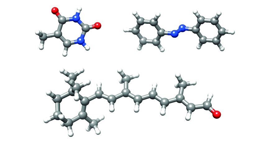
Figure 1: Ground state geometries, optimized at the CCSD/aug-cc-pVDZ level, for thymine (top left), azobenzene (top right), and retinal (bottom).

IV Results and discussion

IV.0.1 Timing Comparisons of Different Implementations

To demonstrate the efficiency of our implementation, we compare calculation times for geometry optimizations of a small system (thymine) and a medium-large system (azobenzene) with the Psi4 and Q-Chem programs. Excited state gradients are not available in Psi4 and thus excited state geometry optimizations have not been performed with this program. We report the percentage of the time spent determining the gradients for the $e^{T}$ calculations. This is not reported for Q-Chem or Psi4, as this time is not directly available from their respective outputs.

Table 3: Ground state calculation times for thymine and azobenzene using Psi4 and our new implementation in $e^{T}$. The number of optimization cycles required, $n_{\mathrm{cycles}}$, are reported, as well as the total calculation time, $t_{\mathrm{total}}$, and the time per cycle, $t_{\mathrm{cycle}}$. The average fraction of time spent calculating the gradient per optimization cycle, $t_{\mathrm{gradient}}$, is reported for $e^{T}$.

	$e^{T}$				Psi4
	$n_{\mathrm{cycles}}$	$t_{\mathrm{total}}$	$t_{\mathrm{cycle}}$	$t_{\mathrm{gradient}}$	$n_{\mathrm{cycles}}$	$t_{\mathrm{total}}$	$t_{\mathrm{cycle}}$
Thymine	6	45m	7m	7 %	7	2h 6m	18m
Azobenzene	11	10h 26m	57m	8.9%	19†	42h 13m	2h 13m

^† The calculation did not converge in 19 cycles in Psi4

Timings for $e^{T}$ and Psi4 are given in Table 3. From the results in the table we see that the calculation of the gradient amounts to only 7%–9% of the total calculation time, illustrating the efficiency of the gradient implementation. Here, the time required to determine the multipliers is not included in the gradient time. We observe that the calculation time required by $e^{T}$, per optimization cycle, is roughly half of that required by Psi4.

When applying an inner projection method, the integral costs are proportional to the size of the auxiliary basis.Folkestad, Kjønstad, and Koch (2019) In the density-fitting scheme used in Psi4, the thymine calculation required 786 auxiliary basis functions, while 967 functions were used in our CD-based implementation. These two numbers are of the same order of magnitude; thus, the computational resources required should be comparable. This is also the case for the azobenzene calculations, in which Psi4 and $e^{T}$ required 1238 and 1444 auxiliary basis functions, respectively. Hence, the two approaches are similar in terms of computational costs. However, note that the time spent on the Cholesky decomposition itself is negligible and that the resulting integral errors are strictly lower than the CD threshold (here $10^{-4}$). Such strict error control is not possible with the density-fitting method.Folkestad, Kjønstad, and Koch (2019)

Table 4: Ground and excited state calculation times for thymine and azobenzene using Q-Chem and our new implementation in $e^{T}$. The excited states are the lowest singlet states in all cases. The number of optimization cycles required, $n_{\mathrm{cycles}}$, are reported, as well as the total calculation time, $t_{\mathrm{total}}$, and the time per cycle, $t_{\mathrm{cycle}}$. The average fraction of time spent calculating the gradient per optimization cycle, $t_{\mathrm{gradient}}$ is reported for $e^{T}$.

	$e^{T}$				Q-Chem
	$n_{\mathrm{cycles}}$	$t_{\mathrm{total}}$	$t_{\mathrm{cycle}}$	$t_{\mathrm{gradient}}$	$n_{\mathrm{cycles}}$	$t_{\mathrm{total}}$	$t_{\mathrm{cycle}}$
Thymine (GS)	6	45m	7m	7 %	10	6h 22m	38m
Thymine (ES)	7	2h 51m	25m	4.5%	7	7h 01m	1h
Azobenzene (GS)	11	10h 26m	57m	8.9%	7	26h 08m	3h 44m
Azobenzene (ES)	10	47h 43m	4h 46m	4.4%	6	37h 40m	6h 17m

Timings for $e^{T}$ and Q-Chem are given in Table 4. We now also consider excited state geometry optimizations, and observe once again that the calculation time is not dominated by the gradient. In fact, the calculation of the gradient amounts to 5% of the full calculation time for the excited state (compared to 10% for the ground state). Note that when reporting the time spent on determining the excited state gradients, we have again excluded the time needed to determine the amplitude response.

From Table 4 it is furthermore observed that we can carry out ground state optimizations in roughly 50% of the time required by Q-Chem, or even less. The savings are significantly larger for ground state optimizations. This can be attributed to differences, between the two programs, in the efficiency of the ground and excited state implementations. The calculation time in Q-Chem can be roughly halved with the utilization of the frozen core approximation (for timings, see SI), resulting in computation times for the excited state that are roughly the same as those observed in $e^{T}$ without this approximation. For the ground state, however, our new implementation still offers significant time savings, despite frozen core calculations being inherently less computationally demanding.

The reported comparisons were carried out without enforcing point-group symmetry. As also noted above, further improvements to the Q-Chem and Psi4 timings could have been obtained by starting from geometries with point-group symmetry.

IV.0.2 Convergence Threshold Effects

In addition to investigating the calculation times, we also studied the effect of changing the CD and gradient convergence thresholds on the final geometry of thymine—as measured by changes in redundant internal coordinates.Bakken and Helgaker (2002) From Table 5 we observe that a very small error is obtained in the final geometry, even at a CD threshold of $10^{-3}$. This small error was also pointed out by Feng et al.Feng et al. (2019) At our chosen CD threshold of $10^{-4}$, the largest change in bond length is less than $0.01$ pm; the changes in angles and dihedral angles are smaller than 0.002 radians, corresponding to about 0.01^∘. Thus, at the CCSD level of theory, the optimized geometry of thymine can be considered fully converged with our chosen CD threshold.

Table 5: Deviations in the optimized geometry of thymine. The deviations are given relative to an optimized geometry obtained with a CD convergence threshold of $10^{-8}$ and a gradient convergence threshold of $3\cdot 10^{-8}$. Changes in internal coordinates are measured by the largest change in a bond length ($\Delta r$), an angle ($\Delta\alpha$), and a dihedral angle ($\Delta\theta$).

CD threshold	Gradient threshold	$\textrm{Max }\Delta r$/pm	$\textrm{Max }\Delta\alpha$/rad	$\textrm{Max }\Delta\theta$/rad
$10^{-3}$	$3\cdot 10^{-3}$	0.043	0.00062	0.0012
$10^{-4}$	$3\cdot 10^{-4}$	0.006	0.00032	0.0012
$10^{-5}$	$3\cdot 10^{-5}$	0.001	0.00002	0.0010

It must be noted, however, that even at this threshold, small differences in the CD basis can occur. This may cause changes in the number of required optimization cycles from run to run, but the final geometries remain unchanged within the specified convergence thresholds.

IV.0.3 Illustration of Large-Scale Application

To showcase the applicability of our implementation, we have also performed a calculation on retinal, which contains 49 atoms and 150 electrons, corresponding to 735 basis functions with our chosen basis set (aug-cc-pVDZ). This calculation was only carried out using $e^{T}$.

Table 6: Calculation time for optimizing the geometry of retainal in $e^{T}$. The number of optimization cycles required, $n_{\mathrm{cycles}}$, are reported, as well as the total calculation time, $t_{\mathrm{total}}$, the time spent per cycle, $t_{\mathrm{cycles}}$, and the average time spent calculating the gradient per optimization cycle, $t_{\mathrm{gradient}}$. The CD convergence threshold was here $10^{-3}$.

	$n_{\mathrm{cycles}}$	$t_{\mathrm{total}}$	$t_{\mathrm{cycle}}$	$t_{\mathrm{gradient}}$
Retinal (GS)	24	17d 10h 23m	17h 26m	6.6%

While the calculation does indeed put a strain on the computational resources, requiring 17 hours per optimization cycle, it can in fact be performed. As in the other calculations, the time spent calculating the gradient amounts to only a small fraction of the total calculation time.

V Conclusions

We have presented an efficient implementation of CCSD gradients for ground and excited states based on Cholesky-decomposed electron repulsion integrals. Since CD is an inner projection scheme, we have chosen an implementation approach that follows earlier schemesBozkaya and Sherrill (2016); Delcey et al. (2014b) for CD and RI where one avoids the storage of $OV^{3}$ and $V^{4}$ arrays by constructing 3-index intermediates. We have furthermore chosen not to store the derivative Cholesky vectors; instead, the associated contributions are constructed on-the-fly. This allows us to significantly reduce the storage requirements.

Relative to Psi4 and Q-Chem, our implementation was shown to reduce the calculation time of geometry optimizations by roughly a factor of two. To a large extent, this reduction in time reflects the efficiency of the coupled cluster code in the $e^{T}$ program. However, the calculation of gradients was found to require only a small fraction of the total calculation time, showcasing the efficiency of the gradient implementation.

The capabilities of our implementation was highlighted by showing that a geometry optimization of retinal could be carried out.

Further reduction in computational demands would be achieved by means of the frozen-core approximation. Work on this is currently in progress.

VI Supplementary material

Comparison of frozen-core and non-frozen-core calculations in Q-Chem.

VII Data availability statement

Geometries can be found in Ref. 54. The code will be released in an upcoming version of the $e^{T}$ program, which is open-source.Folkestad et al. (2020)

Appendix A Two-electron densities

The two-electron density is here taken as

$$d_{pqrs}=L_{\nu}\langle\nu\hskip 1.00006pt|\hskip 1.00006pte^{-T_{2}}e_{pqrs}e^{T_{2}}\hskip 1.00006pt|\hskip 1.00006pt\rho\rangle R_{\rho},$$ (52)

where

$$e_{pqrs}=E_{pq}E_{rs}-\delta_{qr}E_{ps}.$$ (53)

Note that we are using a $T_{1}$-transformed basis, where the $T_{1}$-dependence has been moved into the derivative integrals, as they will be contracted with the density later on. Throughout, we assume a spin-adapted singlet basis, where the kets are expressed in the so-called elementary basis and bras are expressed in the basis biorthonormal to the kets.Helgaker, Jørgensen, and Olsen (2014)

Recall the special cases in equation of motion theory; the ground state is described by

$$L_{0} =1,\quad L_{\mu}=\bar{t}_{\mu},$$ (54)

$$R_{0} =1,\quad R_{\mu}=0,$$ (55)

and the excited states by

$$L_{0} =0,\quad\quad\quad\;L_{\mu}=L_{\mu},$$ (56)

$$R_{0} =-\bm{\bar{t}}^{T}\bm{R},\quad R_{\mu}=R_{\mu}.$$ (57)

Here $\bm{R}$ and $\bm{L}$ are defined for $\mu>0$, and

$$\bm{A}\bm{R} =\omega\bm{R}$$ (58)

$$\bm{A}^{T}\bm{L} =\omega\bm{L}.$$ (59)

In addition, for the excited state, terms with

$$L_{0} =0,\quad L_{\mu}=\bar{t}^{\textrm{ES}}_{\mu}$$ (60)

$$R_{0} =1,\quad R_{\mu}=0$$ (61)

must be determined to account for the terms of the excited state Lagrangian containing the the amplitude response $\bar{\zeta}_{\mu}$. These terms will however be formally identical to the terms of the ground state that do not include $L_{0}$, and these will therefore not be written out explicitly. This applies to both the one- and two-electron densities.

In the following, we shall utilize that $R_{2}$ can be written as $\tilde{R}_{2}$:

$$\begin{split}R_{2}&=\frac{1}{2}\sum_{aibj}R_{aibj}(1+\delta_{ai,bj})E_{ai}E_{bj}\\ &\equiv\frac{1}{2}\sum_{aibj}\tilde{R}_{aibj}E_{ai}E_{bj}=\tilde{R}_{2}.\end{split}$$ (62)

There are eight unique combinations of occupied and virtual indices, because of the symmetry

$$e_{pqrs}=e_{rspq}\implies d_{pqrs}=d_{rspq}.$$ (63)

For each of these combinations, we derive below the corresponding CCSD two-electron density block. For improved readability, Einstein’s implicit summation over repeated indices will be used.

For the ground state we obtain and implement

$$d_{ijkl}^{\textrm{gs}} =(L_{0}R_{0})\Lambda_{ijkl}+O^{(2)}_{ijkl}(L_{2},T_{2})R_{0}$$ (64)

$$d_{aijk}^{\textrm{gs}} =(2L^{a}_{i}\delta_{jk}-L^{a}_{k}\delta_{ji})R_{0}$$ (65)

$$d_{ijka}^{\textrm{gs}} =O^{(M)}_{ijka}(L_{1},T_{2})R_{0}$$ (66)

$$d_{abij}^{\textrm{gs}} =O^{(2)}_{abij}(L_{2},T_{2})R_{0}$$ (67)

$$d_{aibj}^{\textrm{gs}} =L_{ij}^{ab}R_{0}$$ (68)

$$d_{iajb}^{\textrm{gs}} =2R_{0}L_{0}\tilde{t}_{ij}^{ab}+R_{0}\frac{1}{2}O_{iajb}^{(2)}(L_{2},T_{2})$$ (69)

$$d_{aijb}^{\textrm{gs}} =O^{(M)}_{aijb}(L_{2},T_{2})R_{0}$$ (70)

$$d_{abci}^{\textrm{gs}} =0$$ (71)

$$d_{abic}^{\textrm{gs}} =L^{a}_{m}\tilde{t}^{cb}_{im}R_{0}$$ (72)

$$d_{abcd}^{\textrm{gs}} =O^{(2)}_{abcd}(L_{2},T_{2})R_{0}.$$ (73)

and, for the excited state, we similarly obtain and implement

$$\begin{split}d_{ijkl}^{\textrm{es}}&=O^{(2)}_{ijkl}(L_{2},U)+(\bm{L}^{T}\bm{R})\Lambda_{ijkl}\\ &\quad+O_{ijkl}^{[1]}(L_{1},R_{1})\end{split}$$ (74)

$$\begin{split}d_{aijk}^{\textrm{es}}&=(2L^{a}_{i}\delta_{jk}-L^{a}_{k}\delta_{ji})R_{0}-L_{ik}^{ad}R_{dj}\\ &\quad+2W_{ai}\delta_{jk}-W_{ak}\delta_{ji}\end{split}$$ (75)

$$\begin{split}d_{ijka}^{\textrm{es}}&=O^{(M)}_{ijka}(L_{1},U)\\ &\quad-2X_{ij}(L_{2},T_{2})R_{k}^{a}\\ &\quad+X_{kj}(L_{2},T_{2})R_{i}^{a}+X_{da}R_{i}^{d}\delta_{jk}\\ &\quad+\Big{(}V_{djai}(L_{2},T_{2})+Y_{djai}(L_{2},T_{2})\\ &\quad-2\delta_{ij}X_{da}(L_{2},T_{2}))\Big{)}R_{k}^{d}\\ &\quad+\Big{(}Z_{ijkl}(L_{2},T_{2})+X_{il}(L_{2},T_{2})\delta_{jk}\\ &\quad-2\delta_{ij}X_{kl}(L_{2},T_{2}))\Big{)}R_{l}^{a}\\ &\quad-\tilde{t}_{ik}^{ea}W_{ej}-\Big{(}\tilde{t}_{mi}^{ea}\delta_{jk}-2\delta_{ij}\tilde{t}_{mk}^{ea}\Big{)}W_{em}\\ &\quad-\tilde{Y}_{djak}(L_{2},T_{2})R_{i}^{d}\end{split}$$ (76)

$$d_{abij}^{\textrm{es}} =O^{(2)}_{abij}(L_{2},U)+O^{(1)}_{abij}(L_{1},R_{1})$$ (77)

$$d_{aibj}^{\textrm{es}} =L_{ij}^{ab}R_{0}$$ (78)

$$\begin{split}d_{iajb}^{\textrm{es}}&=O_{iajb}^{(2)}(L_{2},U_{2})\\ &\quad+2L_{ck}\tilde{t}_{ik}^{ac}R_{bj}-L_{ck}\tilde{t}_{jk}^{ac}R_{bi}+2L_{ck}\tilde{t}_{jk}^{bc}R_{ai}\\ &\quad-L_{ck}\tilde{t}_{ik}^{bc}R_{aj}-Y_{cb}\tilde{t}_{ij}^{ac}-Y_{ca}\tilde{t}_{ji}^{bc}-Y_{jk}\tilde{t}_{ik}^{ab}\\ &\quad-Y_{ik}\tilde{t}_{kj}^{ab}+2L_{ck}\tilde{t}_{ij}^{ab}R_{ck}+{L_{kl}^{cd}\tilde{R}_{kl}^{cd}\tilde{t}_{ij}^{ab}}\end{split}$$ (79)

$$d_{aijb}^{\textrm{es}} =O^{(M)}_{aijb}(L_{2},U)+2L_{ai}R_{bj}-Y_{ab}\delta_{ij}$$ (80)

$$d_{abci}^{\textrm{es}} =L_{ji}^{ac}R_{j}^{b}$$ (81)

$$\begin{split}d_{abic}^{\textrm{es}}&=L^{a}_{m}\tilde{t}^{cb}_{im}R_{0}\\ &\quad+L_{m}^{a}(2\tilde{R}_{mi}^{bc}-\tilde{R}_{mi}^{cb})\\ &\quad+2X_{ab}(L_{2},T_{2})R_{i}^{c}\\ &\quad-(V_{akbi}(L_{2},T_{2})+Y_{akbi}(L_{2},T_{2}))R_{k}^{c}\\ &\quad+L_{mk}^{ad}\tilde{t}_{mi}^{bc}R_{k}^{d}-L_{mn}^{ad}t_{mn}^{bc}R_{i}^{d}\\ &\quad+{\tilde{Y}_{akci}(L_{2},T_{2})}R_{k}^{b}-X_{ac}(L_{2},T_{2})R_{i}^{b}\end{split}$$ (82)

$$d_{abcd}^{\textrm{es}} =O^{(2)}_{abcd}(L_{2},U).$$ (83)

Here we have defined the following quantities:

$$\Lambda_{ijkl} =4\delta_{ij}\delta_{kl}-2\delta_{il}\delta_{kj}$$ (84)

$$\begin{split}O_{ijkl}^{(1)}(L_{1},R_{1})&=-2Y_{ij}\delta_{kl}+Y_{il}\delta_{kj}\\ &\quad-2\delta_{ij}Y_{kl}+\delta_{il}Y_{kj}\end{split}$$ (85)

$$Y_{kj} =R_{ek}L_{ej}=R_{k}^{e}L_{j}^{e}$$ (86)

$$\begin{split}O_{ijkl}^{(2)}(L_{2},C_{2})&=-2\delta_{kl}X_{ij}(L_{2},C_{2})\\ &\quad-2\delta_{ij}X_{kl}(L_{2},C_{2})\\ &\quad+\delta_{kj}X_{il}(L_{2},C_{2})+\delta_{il}X_{kj}(L_{2},C_{2})\\ &\quad+Z_{ijkl}(L_{2},C_{2})\end{split}$$ (87)

$$X_{ij}(L_{2},C_{2}) =C_{mi}^{ef}L^{ef}_{mj}$$ (88)

$$Z_{ijkl}(L_{2},C_{2}) =C_{ik}^{ef}L^{ef}_{jl}$$ (89)

$$U_{2} =T_{2}\frac{1}{2}R_{0}+\tilde{R}_{2}$$ (90)

$$\begin{split}O^{(M)}_{ijka}(L_{1},T_{2})&=L_{em}\left(2\delta_{ij}\tilde{t}_{km}^{ae}-\delta_{jk}\tilde{t}_{mi}^{ea}\right)R_{0}\\ &\quad-L_{ej}\tilde{t}_{ik}^{ea}R_{0}\end{split}$$ (91)

$$\tilde{Y}_{djak}(L_{2},T_{2}) =L_{mj}^{ed}\tilde{t}_{mk}^{ea}$$ (92)

$$Y_{ab} =L_{k}^{a}R_{k}^{b}$$ (93)

$$O^{(1)}_{abij}(L_{1},R_{1}) =2\delta_{ij}Y_{ab}(L_{1},R_{1})-L_{j}^{a}R_{i}^{b}$$ (94)

$$\begin{split}O^{(2)}_{abij}(L_{2},C_{2})&=2\delta_{ij}X_{ab}(L_{2},C_{2})-Y_{ajbi}(L_{2},C_{2})\\ &\quad-V_{ajbi}(L_{2},C_{2})\end{split}$$ (95)

$$\begin{split}O_{iajb}^{(2)}(L_{2},C_{2})&=\tilde{Y}_{ckai}(L_{2},T_{2})\tilde{C}_{kj}^{cb}\\ &\quad+\tilde{Y}_{ckbj}(L_{2},T_{2})\tilde{C}_{ki}^{ca}\\ &\quad+Z_{ikjl}(L_{2},T_{2})C_{kl}^{ab}\\ &\quad+Z_{imjn}(L_{2},C_{2})t_{mn}^{ab}\\ &\quad-X_{ca}(L_{2},T_{2})\tilde{C}_{ij}^{cb}\\ &\quad-X_{ea}(L_{2},C_{2})\tilde{t}_{ij}^{eb}\\ &\quad-X_{ik}(L_{2},T_{2})\tilde{C}_{kj}^{ab}\\ &\quad-X_{im}(L_{2},C_{2})\tilde{t}_{mj}^{ab}\\ &\quad-X_{jk}(L_{2},T_{2})\tilde{C}_{ik}^{ab}\\ &\quad-X_{jm}(L_{2},C_{2})\tilde{t}_{im}^{ab}\\ &\quad-X_{cb}(L_{2},T_{2})\tilde{C}_{ji}^{ca}\\ &\quad-X_{eb}(L_{2},C_{2})\tilde{t}_{ji}^{ea}\\ &\quad-\tilde{Y}_{embi}(L_{2},C_{2})t_{mj}^{ea}\\ &\quad-Y_{emaj}(L_{2},C_{2})\tilde{t}_{mi}^{eb}\\ &\quad+Y_{ckbi}(L_{2},C_{2})t_{kj}^{ac}\\ &\quad+Y_{ckbi}C_{kj}^{ac}\\ &\quad+V_{ckaj}(L_{2},T_{2})C_{ik}^{cb}\\ &\quad+V_{ckbi}(L_{2},T_{2})C_{kj}^{ac}\end{split}$$ (96)

$$\begin{split}O^{(M)}_{aijb}(L_{2},C_{2})&=-L_{im}^{ae}C_{jm}^{eb}R_{0}\\ &\quad+2Y_{aibj}(L_{2},C_{2})-\delta_{ij}X_{ab}(L_{2},C_{2})\end{split}$$ (97)

$$O^{(2)}_{abcd}(L_{2},C_{2}) =L_{ij}^{ac}C_{ij}^{bd},$$ (98)

where $C_{2}$ denotes a set of double amplitudes and $\tilde{C}_{2}$ is defined in an identical fashion to $\tilde{t}$.

All $O^{4}$, $O^{3}V$ and $O^{2}V^{2}$ densities are directly constructed and stored in memory, while the $OV^{3}$ and $V^{4}$ densities are not explicitly constructed. As discussed in Section II.2, we instead construct their contributions to the 3-index density intermediates $W^{J}_{pq}$ and store these in memory.

Appendix B Orbital relaxation in reorthonormalization

The relaxation contributions—which we derive by expanding $h_{pq}^{(1)}$ and $g_{pqrs}^{(1)}$ using Eq. (21) and inserting into the differentiated Fock matrix, see Eq. (4) and (20)—are

$$\mathcal{F}_{aq}^{\bar{\kappa}} =\frac{1}{2}\bar{\kappa}_{ai}h_{qi}+(g_{qijj}-\frac{1}{2}g_{qjji})\bar{\kappa}_{ai}$$ (99)

$$\begin{split}\mathcal{F}_{iq}^{\bar{\kappa}}&=\frac{1}{2}\bar{\kappa}_{ai}h_{aq}+(g_{aqjj}-\frac{1}{2}g_{ajjq})\bar{\kappa}_{ai}\\ &+2g_{ajqi}\bar{\kappa}_{aj}-\frac{1}{2}g_{aqij}\bar{\kappa}_{aj}-\frac{1}{2}g_{aiqj}\bar{\kappa}_{aj}\end{split}$$ (100)

These terms scale as $O(N^{4})$ once expressed in terms of Cholesky vectors, in terms of which

$$\mathcal{F}_{aq}^{\bar{\kappa}} =\frac{1}{2}\bar{\kappa}_{ai}h_{qi}+\gamma^{J}D_{qa}^{J}-\frac{1}{2}L_{qj}^{J}D_{ja}^{J}$$ (101)

$$\begin{split}\mathcal{F}_{iq}^{\bar{\kappa}}&=\frac{1}{2}\bar{\kappa}_{ai}h_{aq}+E_{qi}^{J}\gamma^{J}\\ &-\frac{1}{2}M_{aq}\bar{\kappa}_{ai}+2\delta^{J}L_{qi}^{J}-\frac{1}{2}E_{qj}^{J}L_{ij}^{J}\\ &-\frac{1}{2}E_{ij}^{J}L_{qj}^{J},\end{split}$$ (102)

where

$$D_{qa}^{J} =L_{qi}^{J}\bar{\kappa}_{ai}$$ (103)

$$\gamma^{J} =L_{jj}^{J}$$ (104)

$$E_{qi}^{J} =L_{aq}^{J}\bar{\kappa}_{ai}$$ (105)

$$M_{aq} =L_{aj}^{J}L_{jq}^{J}$$ (106)

$$\delta^{J} =L_{ai}^{J}\bar{\kappa}_{ai}.$$ (107)

We have used the Einstein’s implicit summation in all these expressions.

References

- Schlegel (2011) H. B. Schlegel, WIREs Comput. Mol. Sci. 1, 790 (2011), https://wires.onlinelibrary.wiley.com/doi/pdf/10.1002/wcms.34 .
- Klippenstein, Pande, and Truhlar (2014) S. J. Klippenstein, V. S. Pande, and D. G. Truhlar, J. Am. Chem. Soc. 136, 528 (2014), https://doi.org/10.1021/ja408723a .
- Marx and Hutter (2009) D. Marx and J. Hutter, Ab initio molecular dynamics: basic theory and advanced methods (Cambridge University Press, 2009).
- Curchod and Martínez (2018) B. F. E. Curchod and T. J. Martínez, Chem. Rev. 118, 3305 (2018), https://doi.org/10.1021/acs.chemrev.7b00423 .
- Čížek (1966) J. Čížek, J. Chem. Phys. 45, 4256 (1966), https://doi.org/10.1063/1.1727484 .
- Bartlett (1981) R. J. Bartlett, Annu. Rev. Phys. Chem 32, 359 (1981), https://doi.org/10.1146/annurev.pc.32.100181.002043 .
- Bartlett (1989) R. J. Bartlett, J. Phys. Chem. 93, 1697 (1989), https://doi.org/10.1021/j100342a008 .
- Crawford and Schaefer III (2000) T. D. Crawford and H. F. Schaefer III, “An introduction to coupled cluster theory for computational chemists,” in Reviews in Computational Chemistry (John Wiley & Sons, Ltd, 2000) pp. 33–136, https://onlinelibrary.wiley.com/doi/pdf/10.1002/9780470125915.ch2 .
- Bartlett and Musiał (2007) R. J. Bartlett and M. Musiał, Rev. Mod. Phys. 79, 291 (2007).
- Helgaker, Jørgensen, and Olsen (2014) T. Helgaker, P. Jørgensen, and J. Olsen, Molecular electronic-structure theory (John Wiley & Sons, 2014).
- Koch et al. (1997) H. Koch, O. Christiansen, P. Jørgensen, A. M. Sanchez de Merás, and T. Helgaker, J. Chem. Phys. 106, 1808 (1997), https://doi.org/10.1063/1.473322 .
- Izsák (2020) R. Izsák, Wiley Interdiscip. Rev. Comput. Mol. Sci 10, e1445 (2020), https://onlinelibrary.wiley.com/doi/pdf/10.1002/wcms.1445 .
- Christiansen, Koch, and Jørgensen (1995) O. Christiansen, H. Koch, and P. Jørgensen, Chem. Phys. Lett. 243, 409 (1995).
- Purvis and Bartlett (1982) G. D. Purvis and R. J. Bartlett, J. Chem. Phys. 76, 1910 (1982), https://doi.org/10.1063/1.443164 .
- Epifanovsky et al. (2021) E. Epifanovsky, A. T. B. Gilbert, X. Feng, J. Lee, Y. Mao, N. Mardirossian, P. Pokhilko, A. F. White, M. P. Coons, A. L. Dempwolff, Z. Gan, D. Hait, P. R. Horn, L. D. Jacobson, I. Kaliman, J. Kussmann, A. W. Lange, K. U. Lao, D. S. Levine, J. Liu, S. C. McKenzie, A. F. Morrison, K. D. Nanda, F. Plasser, D. R. Rehn, M. L. Vidal, Z.-Q. You, Y. Zhu, B. Alam, B. J. Albrecht, A. Aldossary, E. Alguire, J. H. Andersen, V. Athavale, D. Barton, K. Begam, A. Behn, N. Bellonzi, Y. A. Bernard, E. J. Berquist, H. G. A. Burton, A. Carreras, K. Carter-Fenk, R. Chakraborty, A. D. Chien, K. D. Closser, V. Cofer-Shabica, S. Dasgupta, M. de Wergifosse, J. Deng, M. Diedenhofen, H. Do, S. Ehlert, P.-T. Fang, S. Fatehi, Q. Feng, T. Friedhoff, J. Gayvert, Q. Ge, G. Gidofalvi, M. Goldey, J. Gomes, C. E. González-Espinoza, S. Gulania, A. O. Gunina, M. W. D. Hanson-Heine, P. H. P. Harbach, A. Hauser, M. F. Herbst, M. Hernández Vera, M. Hodecker, Z. C. Holden, S. Houck, X. Huang, K. Hui, B. C. Huynh, M. Ivanov, A. Jász, H. Ji, H. Jiang, B. Kaduk, S. Kähler, K. Khistyaev, J. Kim, G. Kis, P. Klunzinger, Z. Koczor-Benda, J. H. Koh, D. Kosenkov, L. Koulias, T. Kowalczyk, C. M. Krauter, K. Kue, A. Kunitsa, T. Kus, I. Ladjánszki, A. Landau, K. V. Lawler, D. Lefrancois, S. Lehtola, R. R. Li, Y.-P. Li, J. Liang, M. Liebenthal, H.-H. Lin, Y.-S. Lin, F. Liu, K.-Y. Liu, M. Loipersberger, A. Luenser, A. Manjanath, P. Manohar, E. Mansoor, S. F. Manzer, S.-P. Mao, A. V. Marenich, T. Markovich, S. Mason, S. A. Maurer, P. F. McLaughlin, M. F. S. J. Menger, J.-M. Mewes, S. A. Mewes, P. Morgante, J. W. Mullinax, K. J. Oosterbaan, G. Paran, A. C. Paul, S. K. Paul, F. Pavošević, Z. Pei, S. Prager, E. I. Proynov, Á. Rák, E. Ramos-Cordoba, B. Rana, A. E. Rask, A. Rettig, R. M. Richard, F. Rob, E. Rossomme, T. Scheele, M. Scheurer, M. Schneider, N. Sergueev, S. M. Sharada, W. Skomorowski, D. W. Small, C. J. Stein, Y.-C. Su, E. J. Sundstrom, Z. Tao, J. Thirman, G. J. Tornai, T. Tsuchimochi, N. M. Tubman, S. P. Veccham, O. Vydrov, J. Wenzel, J. Witte, A. Yamada, K. Yao, S. Yeganeh, S. R. Yost, A. Zech, I. Y. Zhang, X. Zhang, Y. Zhang, D. Zuev, A. Aspuru-Guzik, A. T. Bell, N. A. Besley, K. B. Bravaya, B. R. Brooks, D. Casanova, J.-D. Chai, S. Coriani, C. J. Cramer, G. Cserey, A. E. DePrince, R. A. DiStasio, A. Dreuw, B. D. Dunietz, T. R. Furlani, W. A. Goddard, S. Hammes-Schiffer, T. Head-Gordon, W. J. Hehre, C.-P. Hsu, T.-C. Jagau, Y. Jung, A. Klamt, J. Kong, D. S. Lambrecht, W. Liang, N. J. Mayhall, C. W. McCurdy, J. B. Neaton, C. Ochsenfeld, J. A. Parkhill, R. Peverati, V. A. Rassolov, Y. Shao, L. V. Slipchenko, T. Stauch, R. P. Steele, J. E. Subotnik, A. J. W. Thom, A. Tkatchenko, D. G. Truhlar, T. Van Voorhis, T. A. Wesolowski, K. B. Whaley, H. L. Woodcock, P. M. Zimmerman, S. Faraji, P. M. W. Gill, M. Head-Gordon, J. M. Herbert, and A. I. Krylov, J. Chem. Phys. 155, 084801 (2021).
- Feng et al. (2019) X. Feng, E. Epifanovsky, J. Gauss, and A. I. Krylov, J. Chem. Phys. 151, 014110 (2019), https://doi.org/10.1063/1.5100022 .
- Frisch et al. (2016) M. J. Frisch, G. W. Trucks, H. B. Schlegel, G. E. Scuseria, M. A. Robb, J. R. Cheeseman, G. Scalmani, V. Barone, G. A. Petersson, H. Nakatsuji, X. Li, M. Caricato, A. V. Marenich, J. Bloino, B. G. Janesko, R. Gomperts, B. Mennucci, H. P. Hratchian, J. V. Ortiz, A. F. Izmaylov, J. L. Sonnenberg, D. Williams-Young, F. Ding, F. Lipparini, F. Egidi, J. Goings, B. Peng, A. Petrone, T. Henderson, D. Ranasinghe, V. G. Zakrzewski, J. Gao, N. Rega, G. Zheng, W. Liang, M. Hada, M. Ehara, K. Toyota, R. Fukuda, J. Hasegawa, M. Ishida, T. Nakajima, Y. Honda, O. Kitao, H. Nakai, T. Vreven, K. Throssell, J. A. Montgomery, Jr., J. E. Peralta, F. Ogliaro, M. J. Bearpark, J. J. Heyd, E. N. Brothers, K. N. Kudin, V. N. Staroverov, T. A. Keith, R. Kobayashi, J. Normand, K. Raghavachari, A. P. Rendell, J. C. Burant, S. S. Iyengar, J. Tomasi, M. Cossi, J. M. Millam, M. Klene, C. Adamo, R. Cammi, J. W. Ochterski, R. L. Martin, K. Morokuma, O. Farkas, J. B. Foresman, and D. J. Fox, “Gaussian˜16 Revision C.01,” (2016), gaussian Inc. Wallingford CT.
- Smith et al. (2020) D. G. A. Smith, L. A. Burns, A. C. Simmonett, R. M. Parrish, M. C. Schieber, R. Galvelis, P. Kraus, H. Kruse, R. Di Remigio, A. Alenaizan, A. M. James, S. Lehtola, J. P. Misiewicz, M. Scheurer, R. A. Shaw, J. B. Schriber, Y. Xie, Z. L. Glick, D. A. Sirianni, J. S. O’Brien, J. M. Waldrop, A. Kumar, E. G. Hohenstein, B. P. Pritchard, B. R. Brooks, H. F. Schaefer, A. Y. Sokolov, K. Patkowski, A. E. DePrince, U. Bozkaya, R. A. King, F. A. Evangelista, J. M. Turney, T. D. Crawford, and C. D. Sherrill, J. Chem. Phys. 152, 184108 (2020), https://doi.org/10.1063/5.0006002 .
- Bozkaya and Sherrill (2016) U. Bozkaya and C. D. Sherrill, J. Chem. Phys. 144, 174103 (2016), https://doi.org/10.1063/1.4948318 .
- Aidas et al. (2014) K. Aidas, C. Angeli, K. L. Bak, V. Bakken, R. Bast, L. Boman, O. Christiansen, R. Cimiraglia, S. Coriani, P. Dahle, E. K. Dalskov, U. Ekström, T. Enevoldsen, J. J. Eriksen, P. Ettenhuber, B. Fernández, L. Ferrighi, H. Fliegl, L. Frediani, K. Hald, A. Halkier, C. Hättig, H. Heiberg, T. Helgaker, A. C. Hennum, H. Hettema, E. Hjertenæs, S. Høst, I.-M. Høyvik, M. F. Iozzi, B. Jansík, H. J. Aa. Jensen, D. Jonsson, P. Jørgensen, J. Kauczor, S. Kirpekar, T. Kjærgaard, W. Klopper, S. Knecht, R. Kobayashi, H. Koch, J. Kongsted, A. Krapp, K. Kristensen, A. Ligabue, O. B. Lutnæs, J. I. Melo, K. V. Mikkelsen, R. H. Myhre, C. Neiss, C. B. Nielsen, P. Norman, J. Olsen, J. M. H. Olsen, A. Osted, M. J. Packer, F. Pawlowski, T. B. Pedersen, P. F. Provasi, S. Reine, Z. Rinkevicius, T. A. Ruden, K. Ruud, V. V. Rybkin, P. Sałek, C. C. M. Samson, A. S. de Merás, T. Saue, S. P. A. Sauer, B. Schimmelpfennig, K. Sneskov, A. H. Steindal, K. O. Sylvester-Hvid, P. R. Taylor, A. M. Teale, E. I. Tellgren, D. P. Tew, A. J. Thorvaldsen, L. Thøgersen, O. Vahtras, M. A. Watson, D. J. D. Wilson, M. Ziolkowski, and H. Ågren, WIREs Comput.Mol.Sci. 4, 269 (2014).
- Hald et al. (2003) K. Hald, A. Halkier, P. Jørgensen, S. Coriani, C. Hättig, and T. Helgaker, J. Chem. Phys. 118, 2985 (2003), https://doi.org/10.1063/1.1531106 .
- Matthews et al. (2020) D. A. Matthews, L. Cheng, M. E. Harding, F. Lipparini, S. Stopkowicz, T.-C. Jagau, P. G. Szalay, J. Gauss, and J. F. Stanton, J. Chem. Phys. 152, 214108 (2020), https://doi.org/10.1063/5.0004837 .
- Gauss, Stanton, and Bartlett (1991) J. Gauss, J. F. Stanton, and R. J. Bartlett, J. Chem. Phys. 95, 2623 (1991), https://doi.org/10.1063/1.460915 .
- Kállay et al. (2020) M. Kállay, P. R. Nagy, D. Mester, Z. Rolik, G. Samu, J. Csontos, J. Csóka, P. B. Szabó, L. Gyevi-Nagy, B. Hégely, I. Ladjánszki, L. Szegedy, B. Ladóczki, K. Petrov, M. Farkas, P. D. Mezei, and Á. Ganyecz, J. Chem. Phys. 152, 074107 (2020), https://doi.org/10.1063/1.5142048 .
- Kállay, Gauss, and Szalay (2003) M. Kállay, J. Gauss, and P. G. Szalay, J. Chem. Phys. 119, 2991 (2003), https://doi.org/10.1063/1.1589003 .
- Beebe and Linderberg (1977) N. H. F. Beebe and J. Linderberg, Int. J. Quantum Chem 12, 683 (1977), https://onlinelibrary.wiley.com/doi/pdf/10.1002/qua.560120408 .
- Røeggen and Wisløff-Nilssen (1986) I. Røeggen and E. Wisløff-Nilssen, Chem. Phys. Lett. 132, 154 (1986).
- Koch, Sánchez de Merás, and Pedersen (2003) H. Koch, A. Sánchez de Merás, and T. B. Pedersen, J. Chem. Phys. 118, 9481 (2003), https://doi.org/10.1063/1.1578621 .
- Aquilante, Pedersen, and Lindh (2007) F. Aquilante, T. B. Pedersen, and R. Lindh, J. Chem. Phys. 126, 194106 (2007), https://doi.org/10.1063/1.2736701 .
- DePrince and Sherrill (2013) A. E. DePrince and C. D. Sherrill, J. Chem. Theory Comput 9, 293 (2013), https://doi.org/10.1021/ct300780u .
- Bozkaya (2014) U. Bozkaya, J. Chem. Theory Comput. 10, 2371 (2014), https://doi.org/10.1021/ct500231c .
- Delcey et al. (2014a) M. G. Delcey, L. Freitag, T. B. Pedersen, F. Aquilante, R. Lindh, and L. González, J. Chem. Phys. 140, 174103 (2014a), https://doi.org/10.1063/1.4873349 .
- Folkestad, Kjønstad, and Koch (2019) S. D. Folkestad, E. F. Kjønstad, and H. Koch, J. Chem. Phys. 150, 194112 (2019), https://doi.org/10.1063/1.5083802 .
- Whitten (1973) J. L. Whitten, J. Chem. Phys. 58, 4496 (1973), https://doi.org/10.1063/1.1679012 .
- Dunlap, Connolly, and Sabin (1979) B. I. Dunlap, J. W. D. Connolly, and J. R. Sabin, J. Chem. Phys. 71, 3396 (1979), https://doi.org/10.1063/1.438728 .
- Feyereisen, Fitzgerald, and Komornicki (1993) M. Feyereisen, G. Fitzgerald, and A. Komornicki, Chem. Phys. Lett. 208, 359 (1993).
- Vahtras, Almlöf, and Feyereisen (1993) O. Vahtras, J. Almlöf, and M. Feyereisen, Chem. Phys. Lett. 213, 514 (1993).
- Rendell and Lee (1994) A. P. Rendell and T. J. Lee, J. Chem. Phys. 101, 400 (1994), https://doi.org/10.1063/1.468148 .
- Weigend (2002) F. Weigend, Phys. Chem. Chem. Phys. 4, 4285 (2002).
- Sodt, Subotnik, and Head-Gordon (2006) A. Sodt, J. E. Subotnik, and M. Head-Gordon, J. Chem. Phys. 125, 194109 (2006), https://doi.org/10.1063/1.2370949 .
- Werner, Manby, and Knowles (2003) H.-J. Werner, F. R. Manby, and P. J. Knowles, J. Chem. Phys. 118, 8149 (2003), https://doi.org/10.1063/1.1564816 .
- Schütz and Manby (2003) M. Schütz and F. R. Manby, Phys. Chem. Chem. Phys. 5, 3349 (2003).
- Werner and Schütz (2011) H.-J. Werner and M. Schütz, J. Chem. Phys. 135, 144116 (2011), https://doi.org/10.1063/1.3641642 .
- Folkestad et al. (2020) S. D. Folkestad, E. F. Kjønstad, R. H. Myhre, J. H. Andersen, A. Balbi, S. Coriani, T. Giovannini, L. Goletto, T. S. Haugland, A. Hutcheson, I.-M. Høyvik, T. Moitra, A. C. Paul, M. Scavino, A. S. Skeidsvoll, Å. H. Tveten, and H. Koch, J. Chem. Phys. 152, 184103 (2020), https://doi.org/10.1063/5.0004713 .
- Helgaker and Jørgensen (1992) T. Helgaker and P. Jørgensen, “Calculation of geometrical derivatives in molecular electronic structure theory,” in Methods in Computational Molecular Physics, edited by S. Wilson and G. H. F. Diercksen (Springer US, Boston, MA, 1992) pp. 353–421.
- Helgaker and Jørgensen (1989) T. Helgaker and P. Jørgensen, Theoret. Chim. Acta 75, 111 (1989), doi.org/10.1007/BF00527713 .
- Jørgensen and Helgaker (1988) P. Jørgensen and T. Helgaker, J. Chem. Phys. 89, 1560 (1988), https://doi.org/10.1063/1.455152 .
- Helgaker and Jørgensen (1988) T. Helgaker and P. Jørgensen, Adv. Quant. Chem. 19, 183 (1988).
- Helgaker et al. (2012) T. Helgaker, S. Coriani, P. Jørgensen, K. Kristensen, J. Olsen, and K. Ruud, Chem. Rev. 112, 543 (2012).
- Scheiner et al. (1987) A. C. Scheiner, G. E. Scuseria, J. E. Rice, T. J. Lee, and H. F. Schaefer, J. Chem. Phys. 87, 5361 (1987), https://doi.org/10.1063/1.453655 .
- Scuseria, Janssen, and Schaefer (1988) G. E. Scuseria, C. L. Janssen, and H. F. Schaefer, J. Chem. Phys. 89, 7382 (1988), https://doi.org/10.1063/1.455269 .
- Banerjee et al. (1985) A. Banerjee, N. Adams, J. Simons, and R. Shepard, J. Phys. Chem. 89, 52 (1985).
- Bakken and Helgaker (2002) V. Bakken and T. Helgaker, J. Chem. Phys. 117, 9160 (2002), https://doi.org/10.1063/1.1515483 .
- Schnack-Petersen et al. (2022) A. K. Schnack-Petersen, H. Koch, S. Coriani, and E. F. Kjønstad, (2022), https://doi.org/10.5281/zenodo.5957852.
- Delcey et al. (2014b) M. G. Delcey, L. Freitag, T. B. Pedersen, F. Aquilante, R. Lindh, and L. González, J. Chem. Phys. 140, 174103 (2014b), https://doi.org/10.1063/1.4873349 .