The devil is in the labels: Semantic segmentation from sentences

Abstract

We propose an approach to semantic segmentation that achieves state-of-the-art supervised performance when applied in a zero-shot setting. It thus achieves results equivalent to those of the supervised methods, on each of the major semantic segmentation datasets, without training on those datasets. This is achieved by replacing each class label with a vector-valued embedding of a short paragraph that describes the class. The generality and simplicity of this approach enables merging multiple datasets from different domains, each with varying class labels and semantics. The resulting merged semantic segmentation dataset of over 2 Million images enables training a model that achieves performance equal to that of state-of-the-art supervised methods on $7$ benchmark datasets, despite not using any images therefrom. By fine-tuning the model on standard semantic segmentation datasets, we also achieve a significant improvement over the state-of-the-art supervised segmentation on NYUD-V2 and PASCAL-context at $60\%$ and $65\%$ mIoU, respectively. Based on the closeness of language embeddings, our method can even segment unseen labels.

Extensive experiments demonstrate strong generalization to unseen image domains and unseen labels, and that the method enables impressive performance improvements in downstream applications, including depth estimation and instance segmentation.

1 Introduction

Semantic segmentation is a core problem in computer vision, with broad applications in autonomous driving, agriculture robotics, and medicine. It is also an important precursor to a range of downstream applications including scene understanding, and a host of image and video editing operations. Current deep learning methods have achieved tremendous success through supervised training on a specific high-quality dataset with per-pixel labels for a limited set of classes [13, 28]. These datasets have been created at a great cost, however, and naturally the models trained on them are limited to the classes and image domains represented therein. Training models on these datasets individually inevitably limits the methods’ ability to generalize to unseen image domains and labels. We show here that it is possible to largely mitigate this limitation.

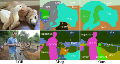
Figure 1: Examples of segmenting zero-shot labels on web images. The labels ‘duck’ (first row) and ‘deer’ (second row) are not in the training data for Mseg [26], or the proposed method. Note that our proposed method is able to segment unseen labels successfully, however.

Training on multiple datasets from multiple domains is a natural way to increase a model’s robustness to variation in the statistics of data, and to improve generalization. Lambert et al. [26] demonstrated that simply training on merged datasets may not drive the desired performance improvements, however, as different datasets can have conflicting label taxonomies. Different datasets may thus have different definitions for the same class, or use different labels to indicate classes with similar semantics. Lambert et al. [26] proposed an effective, yet somewhat laborious solution, requiring re-labeling a merged dataset according to a manually created unified label-set. This is particularly challenging when datasets have semantic classes that need to be split to achieve consistency, as it requires manually identifying a new class label for every segmentation. Lambert et al. applied this approach to $7$ segmentation datasets to build a new merged dataset, named Mseg [26]. The variation in the constituent datasets helps models trained on Mseg achieve robustness to image-domain changes, although this is limited to the fixed set of classes present in the merged taxonomy.

Rather than attempting to manually unify a diverse set of taxonomies, and the corresponding labelled instances, here we propose a method for automatically merging datasets by replacing the labels therein. More specifically, for each category in each dataset, we identify a sentence describing the semantic meaning of the class. These sentences can be manually generated, but in this work are retrieved from Wikipedia. An embedding is then generated from each sentence using a language model.

In this work, we use the language model from CLIP [38], but note that no image information is passed to the model, only the label sentences. Using the resulting vector-valued sentence embeddings as labels allows multiple datasets to be merged without manual intervention or inspection. Our experiments below demonstrate that there is a performance advantage in using sentence-embedding labels for a single dataset, but the primary benefit is that it enables training on more data, from a wider variety of domains, than any single dataset can support.

By merging 9 datasets, we gain access to about 2 Million training images, which span multiple domains. These datasets have a variety of annotation styles, however, ranging from per-pixel labels to bounding boxes. To exploit these varying annotations, we propose a heterogeneous loss that enables to leverage the noisy OpenImages [2] and weakly annotated Objects365 [42]. Our method not only significantly improves model performance and generalization ability to various domains, but also offers the advantage that the resulting model is able to generalize to unseen labels. This can be achieved simply by generating a new sentence describing the new class, and calculating its vector-valued embedding. Applying this new vector label within the already trained model enables zero-shot segmentation of the corresponding class. Figure 1 shows some zero-shot semantic segmentation examples.

As mentioned, the sentence labels used to merge the datasets are retrieved from Wikipedia. The corresponding increase in the volume of training data available is what drives the improvement in both zero-shot, and fully supervised performance to the point where both are significantly beyond the current state-of-the-art methods. Figure 3 provides a visualization of the benefit of sentence-valued class labels even when the classes themselves do not overlap. The block-diagonal nature of the similarity matrix for sentence label embeddings illustrates the fact that this approach better identifies semantic similarities between classes than using an embedding of a single word class label.

The semantic segmentation method that we propose here is able to exploit diverse datasets in training, and which generates state-of-the-art zero-shot and fully-supervised performance as a result. The resulting model boosts the performance of downstream applications such as depth estimation and instance segmentation. Our main contributions are thus as follows.

• We propose an approach for easily merging multiple datasets together by replacing labels with vector-valued sentence embeddings, and use the approach to construct a large semantic segmentation dataset of around 2 Million images.

• The semantic segmentation model trained on this combined dataset achieves state-of-the-art performance on 4 zero-shot datasets. When applied in a supervised setting (by fine-tuning), we surpass the state-of-the-art methods by over 5% on Pascal Context [17] and NYUDv2 [44]. Furthermore, our methods show the significant advantage of segmenting unseen labels.

• To solve the unbalanced annotations quality of mixed datasets, we propose a heterogeneous loss to accommodate the label noise from OpenImages [2] and leverage weakly annotated Objects365 [42].

• With the created pseudo mask labels from our model, the monocular depth estimation accuracy is improved consistently over 5 zero-shot testing datasets. Furthermore, we can surpass the fully-supervised instance segmentation method with only 25% labelled images on the COCO dataset [28].

2 Related Work

Semantic Segmentation. Semantic segmentation requires per-pixel semantic labeling, and as such represents one of the fundamental problems in computer vision. The first fully convolutional approach proposed was FCN [32], and various schemes have been developed for improving upon it. The constant increase in network capacity has driven ongoing improvements in performance on public semantic segmentation benchmarks, driven by developments such as ResNet and Transformer. Recently, stronger transformer backbones such as Segformer [56], Swin [31] have shown promises for semantic segmentation. Researchers have developed various segmentation models by, e.g., investigating larger receptive fields, and exploiting contextual information.

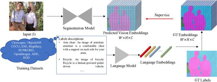
Figure 2: Our framework. We merge multiple datasets together and encode all labels to embeddings using a language model. The semantic segmentation model is enforced to learn pixel-wise embeddings. During testing, the cosine similarity between the predicted embedding and the search embedding space is calculated. The output class is the most similar one in the label space.

Zero-shot Semantic Segmentation. Xian et al. [54] proposed the first zero-shot semantic segmentation method, which transfers knowledge from trained classes to unknown classes based on inter-class similarity. A variety of zero-shot methods have followed [68, 21, 34, 5]. Existing methods are primarily either generative or discriminative. Zhao et al. [68] proposed a discriminative method to solve the zero-shot semantic segmentation problem using a label hierarchy. They thus incorporate hypernym/hyponym relations from WordNet [34] to help with zero-shot parsing. Hu et al. [21] argued that the noisy training data from seen classes challenge the zero-shot label transfer. To address this issue, they proposed an approach based on Bayesian uncertainty estimation. Baek et al. [1] proposed to align the visual and semantic information through a learned joint embedding space, and introduce boundary-aware regression and semantic consistency losses to learn discriminative features. In contrast, some generative methods introduce multi-stage training and fine-tune the classifier on novel unseen classes. Bucher et al. [5] proposed the first generative method (ZS3Net). To create diverse and context-aware features from semantic word embeddings, Gu et al. [19] proposed a contextual module to capture the pixel-wise contextual information in CaGNet.

The term zero-shot has multiple meanings, including both applying a model to a dataset that it has not been trained on [26, 66], and using a pre-trained model to identify novel object classes [54, 21]. The approach that we propose is applicable to both versions of the zero-shot problem. We demonstrate robust performance in both settings. It is most notable, however, that our method achieves a level of accuracy on each of the $7$ major datasets, without training on them, that matches that of the fully-supervised approaches.

Domain-agnostic Dense Prediction. There have been a range of methods that merge segmentation datasets to improve performance and generalization, including Ros et al. [41] who combined six driving datasets, and Bevandic et al. [3] who aggregated four datasets for joint segmentation and outlier detection on WildDash [66] (a benchmark designed for cross-domain robustness evaluation). As mentioned above, Lambert et al. [26] proposed a method for creating a consistent taxonomy to unite datasets from multiple domains. They achieve strong generalization over multiple zero-shot datasets.

Encoding Labels for Zero-shot Learning. Many zero-shot methods have generated semantic embeddings for class labels, and multiple methods for mapping between semantic embeddings and visual features have been devised. For example, Bucher et al. [5] use Word2Vec [33] to encode the labels, and is the only example that we are aware of in semantic segmentation. Recent examples that apply this approach for other purposes include Bujwid et al. [6] and CLIP [38].

3 Our Method

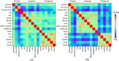
Figure 3: A visualisation of the pairwise distances between label embeddings for (a) single word class labels and (b) sentences. The embeddings of sentence labels better reflect the underlying semantic similarity between classes. For example, classes in ‘Animals’ are close to each other but far from those in ‘People’ and ‘Transport’. Capturing and exploiting these semantic similarities in diverse datasets to be brought to bear to improve both zero-shot, and fully supervised segmentation performance.

Figure 2 shows the overview of our method. Current semantic segmentation methods feed an RGB image $I\in{\cal R}^{W\times H\times 3}$ to a fully convolutional neural network, which predicts per-pixel categories $p\in{\cal R}^{W\times H\times N}$, where $N$ is the number of predetermined categories.

Recently, CLIP [38] shows promising robustness by leveraging natural language supervision for image classification on a large-scale dataset. Inspired by this, instead of using one-hot vectors to represent the predefined labels, we employ language models to encode semantic labels into embedding vectors. In our experiments, we use the CLIP-ViT language model to encode all labels. The encoded language embeddings are $e\in{{\cal R}}^{N\times C}$, where $C$ is the embedding dimension. The vision embeddings from the segmentation model are $\mathcal{V}=\phi(I)\in{\cal R}^{W\times H\times C}$.

Creating Language Embeddings. To train a robust model, we merged multiple datasets together for training. There are $238$ labels in total. Lambert et al. [26] solve this problem by manually create a unified label list and encode each label in a one-hot vector. All labels are independent to each other. In contrast, we employ a soft semantic embedding to replace the original labels, which can retain the relations among labels. Such relations are important for the zero-shot labels semantic segmentation.

Ideally, the closeness between embeddings is positively correlated to the similarity between different labels. For example, ‘Pedestrian’ should be close to ‘Rider’ but far from ‘Animals’ and other objects. Recently, several zero-shot semantic segmentation and classification methods [5, 1, 21] explore pre-trained linguistic semantic features using class names (i.e., word2vec). The problem is that words are sensitive to linguistic issues and can give little discriminability of classes. Some names may partially overlap or not well reflect semantic similarity. For example, ‘counter’ can be a counting device or a long flat-topped fitment. By contrast, textual descriptions are rich in context information. We thus collect short descriptions from Wikipedia to represent each label. For example, ‘bus: An image of bus. A bus is a road vehicle designed to carry many passengers.’ Figure 3 visualizes the cosine similarity matrix of embeddings, which are created from words or sentences. The block-diagonal nature demonstrates that our sentences embeddings better represent the semantic similarities. For example, classes in ‘Animals’ are close to each other but far from those in ‘People’ and ‘Transport’.

Heterogeneous Constraints for Mixed Data Training. To obtain a robust segmentation model, we merge 9 datasets for training, including 7 well-annotated datasets, a coarsely-annotated dataset (OpenImages [2]), and a weakly annotated dataset (Objects365 [42]). Owing to the unbalanced quality, we propose to employ heterogeneous losses to train the model.

For the well annotated dataset, we enforce a pixel-wise loss on all samples. The loss function is as follows: $e$ is the created language embeddings of training labels, while $\mathcal{V}$ is the predicted vision embeddings.

$$\begin{split}z_{i,j}=\frac{e_{j}\cdot\mathcal{V}_{i}}{\left\|e_{j}\right\|\left\|\mathcal{V}_{i}\right\|},i\in[0,M],j\in[0,N]\end{split}$$ (1)

$$\begin{split}l_{i}=\frac{\exp(z_{i,j}/\tau)}{\sum_{j=0}^{N}\exp(z_{i,j}/\tau)}\end{split}$$ (2)

$$\begin{split}L_{\rm HD}=-\frac{1}{M}\sum_{i=0}^{M}y_{i}\log(l_{i})\end{split}$$ (3)

where $M$ is the number of valid pixels, $N$ is the number of categories, $y_{i}$ is the ground-truth label embedding, and $\tau$ is the learnable temperature.

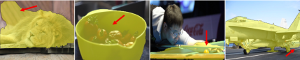
Figure 4: Examples of noisy annotations from OpenImages (see red arrows regions). Left to right: masks for lion, bowl, billiard table, airplane.

As a coarsely annotated dataset contains many noises, we observe that directly enforcing the above pixel-wise loss leads to worse results. Figure 4 shows some noisy annotations from the OpenImages dataset. To alleviate the effect from such noises, we propose to enforce the loss on some high-confident samples and ignore the most noisy parts. The loss functions are as follows:

$$\begin{split}w_{i}=\left\{\begin{matrix}0,|\log(l_{i})|>\mu\\ 1,|\log(l_{i})|\leq\mu\end{matrix}\right.\end{split}$$ (4)

$$\begin{split}L_{\rm LD}=-\frac{1}{M}\sum_{i=0}^{M}w_{i}\cdot y_{i}\log(l_{i}),\end{split}$$ (5)

where $\mu$ is an adaptive threshold. In our experiments, we rank all samples’ losses of each image and set $\mu$ to the highest 30% loss value. Each image has an adaptive threshold. With the proposed heterogeneous loss for OpenImages, we can obtain much better segments (see Figure 7).

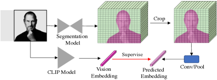
Figure 5: Distillation pipeline. We use the clip classification model to obtain the vision embedding for the bounding box regions. It is applied to supervise the predicted bounding box embedding.

Apart from the pixel-wise supervision, we propose a distillation method to leverage the weakly annotated dataset, such as Objects365, which only contains bounding boxes for foreground objects. Specially, since the CLIP classification model has obtained robust knowledge for image contents, we distill such knowledge to our segmentation model on box-level annotations. We crop and resize the bounding box from the image $I_{r}=(crop(I,r))$ and feed it to the CLIP classification model to obtain the vision embedding for objects, $\mathcal{V}^{*}_{r}=\mathcal{G}(I_{r})$. $I$ is the image and $r$ is the bounding box. To retrieve the predicted bounding box embedding, we crop the corresponding region $crop(\mathcal{V},r)$ from the segmentation embeddings and enforce a $1\times 1$ convolution and ROI pooling on that $\mathcal{V}_{r}={\rm RoI}(crop(\mathcal{V},r))$. Lastly, we apply the $\ell_{1}$ loss to minimize their distance. The pipeline is shown in Figure 5.

$$\begin{split}\textbf{v}^{*}_{r}=\frac{\mathcal{V}^{*}_{r}}{\left\|\mathcal{V}^{*}_{r}\right\|},\textbf{v}_{r}=\frac{\mathcal{V}_{r}}{\left\|\mathcal{V}_{r}\right\|}\end{split}$$ (6)

$$\begin{split}L_{\rm WD}=\frac{1}{P}\sum_{r}^{P}\left\|\textbf{v}^{*}_{r}-\textbf{v}_{r}\right\|_{1}\end{split}$$ (7)

where $P$ is the number of bounding boxes.

The overall loss is as follows:

$$L=L_{\rm HD}+L_{\rm LD}+L_{\rm WD},$$ (8)

During inference, we calculate the cosine similarity between predicted vision embeddings and created language embeddings to obtain pixel-wise labels.

4 Experiments

4.1 Datasets and Implementation Details

In our experiments, we merged multiple datasets together for training and tested on 13 zero-shot datasets to evaluate the robustness of our method.

Training Data. Following Mseg [26], we firstly merged 7 high-quality annotated semantic segmentation datasets (HD), including ADE20K [70], Mapillary [36], COCO Panoptic [28], India Driving Dataset (IDD) [50], BDD100K (BDD) [63], Cityscapes [13], and SUNRGBD [45]. Apart from that, we sample some data from the instance segmentation dataset OpenImagesV6 [2] (OI) and weakly annotated dataset Objects365 [42] (OB) for training. Note that OpenImagesV6 only contains noisy foreground objects masks, while Objects365 provides objects bounding box annotations. These high-quality datasets (HD) have over 200K images. OpenImagesV6 has around 700K images, while Objects365 has over 1M images.

Testing data for Semantic Segmentation		Testing Data for Downstream Applications
CamVid [4]	Test set	Depth Estimation
Pascal VOC [17]	Validation set	NYUv2	Test set
Pascal Context [35]	Validation set	KITTI	Test set
KITTI [18]	Test set	DIODE [51]	Test set
Wilddash1 [66]	Validation set	ScanNet [14]	Validation set
Wilddash2 [66]	Test set	Sintel [7]	Validation set
Youtube VIS [58]	Sampled data	Instance Segmentation
NYUv2 [44]	Test set	COCO [28]	Validation set

Table 1: Datasets employed in our experiments for evaluation.

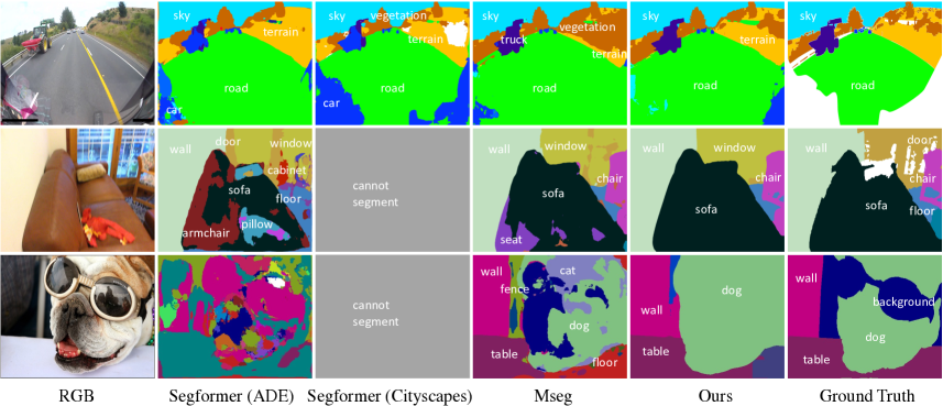
Figure 6: Qualitative comparison on some zero-shot datasets (Pascal Context, ScanNet, and Wilddash1). Comparing with current methods, our method can retrieve better results.

Testing Data for Semantic Segmentation. To evaluate the robustness and effectiveness of our semantic segmentation method, we test on 8 zero-shot datasets, including CamVid [4], KITTI, Pascal VOC, Pascal Context, ScanNet [14], WildDash1 [66], WildDash2 [66], YoutubeVIS [58]. Furthermore, we fine-tune our well-trained model on NYUv2 [44] and Pascal Context to show our method can provide strong performance.

Testing Data for Downstream Applications. We create pseudo semantic labels on zero-shot datasets to boost downstream applications, including the instance segmentation and monocular depth estimation. We create pseudo instance masks on Objects365 to help instance segmentation on COCO [28]. For depth estimation, following LeReS [62], we create pseudo semantic masks on 9 RGBD datasets, of which 4 datasets are employed for training and others are for zero-shot depth evaluation, including NYUDv2, KITTI, DIODE [51], ScanNet, and Sintel [7]. More details are shown in Table 1.

Evaluation Metrics. We employ the mean intersection over union (mIoU) to evaluate semantic segmentation results and AP [28] for the instance segmentation. To evaluate depth quality, following [40, 62], we take absolute relative error (AbsRel) and percentage of pixels satisfying $\delta_{\tau}=\max\left(\frac{d_{pred}}{d_{gt}},\frac{d_{gt}}{d_{pred}}\right)<\tau$ for evaluation.

Implementation Details. We use two network architectures in our experiments, HRNet-W48 [46] and Segformer [56]. When training HRNet, we use SGD with momentum and polynomial learning rate decay, starting with a learning rate of 0.01. For the Segformer network, we use AdamW with polynomial learning rate decay and the initial learning rate 0.00006. To train a robust model on multiple datasets, following [60], we balance all datasets in a mini-batch to ensure each dataset accounts for almost equal ratio. During training, images from all datasets are resized such that their shorter edge is resized to 1080. We randomly crop the image by $713\times 713$ for HRNet and by $640\times 640$ for Segformer. Other data augmentation methods are also applied, including randomly flip, color transformations, image blur, image corruption. In the inference, we resize the image with the short edge to one of three resolutions (480$/$720$/$1080). When comparing with existing methods, multi-scale (ms) or single-scale (ss) testing are employed.

Test on the validation set of training data (mIoU, ss)
Methods	Training Data	COCO	ADE	Mapillary	IDD	BDD	Cityscapes	SUN
Mseg(HRNet)	HD	48.6	42.8	51.9	61.8	63.5	76.3	46.1
Ours(HRNet)	HD	51.5	47.2	51.4	64.3	67.7	78.7	49.1
Ours(HRNet)	HD+OB	53.8	47.6	55.6	65.8	68.6	79.6	46.2
Ours(HRNet)	HD+OI	53.3	48.4	55.3	65.0	69.0	79.2	50.5
Ours(Segformer)	HD	64.0	55.1	57.4	66.3	69.8	82.7	50.4
Ours(Segformer)	HD+OI+OB	64.6	55.1	59.1	67.0	70.5	82.9	50.5

Table 2: Quantitative comparison of our method with Mseg on the validation set of training data. Our method achieves better performance than them over all datasets.

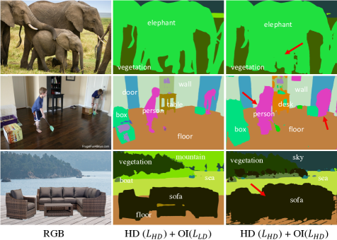
Figure 7: Effectiveness of heterogeneous loss. We test on some google images. With the proposed heterogeneous loss, the segmented results are much more accurate. Red Arrows highlight some comparisons.

4.2 Semantic Segmentation Evaluation

To demonstrate the robustness and effectiveness of our methods, we conduct evaluation on 15 datasets.

Test on zero-shot datasets (mIoU)
Methods	Arch.	Training Data	CamVid†	KITTI‡	VOC‡	Pascal Context‡	ScanNet†	Wildash1‡	Wildash2‡	Mean
PSPNet [69]	ResNet101	*	77.6	-	79.6	47.2	47.5	-	-	-
Liu et al. [30]	ResNet101	*	79.4	-	-	-	-	-	-	-
Zhu et al. [71]	Xception	*	81.7	-	-	-	-	-	-	-
DeepLabV3	ResNet101	*	-	-	79.2	54.0	50.0	-	-	-
DeepLabV3+	ResNet101	*	-	-	77.9	54.5	-	-	-	-
AutoDeeplab [29]	ResNet101	*	-	-	82.0	-	-	-	-	-
HRNet[46]	HRNet-W48	*	-	-	78.6	52.8	-	47.5♮	-	-
3DMV+ [15]	ResNet101	*	-	-	-	-	49.8	-	-	-
SegStereo [57]	-	*	-	59.1	-	-	-	-	-	-
Chroma UDA [16]	ResNet-101	*	-	60.4	-	-	-	-	-	-
SGDepth [25]	ResNet-101	*	-	53.0	-	-	-	-	-	-
Zhang et al. [67]	ResNet-101	*	-	-	-	54.0	-	-	-	-
Porzi [37]	-	*	-	-	-	-	-	-	37.1	-
VideoGCRF [9]	ResNet101	*	75.2	-	-	-	-	-	-	-
Segformer [56]	Segformer-B5	Cityscapes	-	-	-	-	-	50.2♮	-	-
Valada et al. [48]	ResNet50	*	-	-	-	-	52.9	-	-	-
Mseg [26]	HRNet-W48	HD	82.4	62.4	70.8	45.2	48.4	64.2	34.6	58.2
Ours	HRNet-W48	HD	82.8	63.8	71.6	45.8	46.3	63.4	34.4	58.3
Ours	HRNet-W48	HD+OB	83.4	66.0	74.6	48.3	49.8	63.4	35.0	60.1
Ours	HRNet-W48	HD+OI	83.4	66.9	74.9	48.6	52.0	64.0	35.7	60.8
Ours	Segformer-B5	HD	83.6	66.5	79.9	53.0	53.0	68.2	37.2	63.1
Ours	Segformer-B5	HD+OI+OB	83.7	68.9	81.1	54.2	55.3	69.7	37.9	64.4

^† Single-scale results. ^‡ Multi-scale results. $*$ Methods are trained on the corresponding training set. ^♮ Models are trained on Cityscapes.

Table 3: Quantitative comparison of our semantic segmentation with state-of-the-art methods on 7 zero-shot (unseen during training) datasets. Our method achieves better performance than existing state-of-the-art methods on CamVid, ScanNet, WildDash, and WildDash2, and is on par with existing methods on other 3 datasets.

Zero-shot Cross-domain Transfer Evaluation. In this experiment, we aim to evaluate the zero-shot generalization over multiple datasets. We compare with current state-of-the-art methods on 7 zero-shot datasets (unseen to our method during training). Mseg [26] is trained on 7 well-annotated datasets and has demonstrated strong generalization over multiple datasets, while other methods are well-trained on the corresponding training set. Results are shown in Table 3. Comparing to previous methods, our method can achieve state-of-the-art performance on CamViD, ScanNet, WildDash1, and WildDash2. Although other datasets are unseen to our method during training, we can achieve comparable performance with existing methods. Comparing with Mseg, we use embeddings to encode labels can achieve comparable performance with the HRNet-W48 backbone. Furthermore, when using stronger transformer backbone (segformer [56]), the performance is improved consistently over all datasets.

Effectiveness of Heterogeneous Constraints. We propose the heterogeneous loss to supervise the merged datasets. When aggregating OpenImages (‘HD+OI’) supervised with our $L_{\rm HD}+L_{\rm LD}$, Table 3 shows the performance can be improved consistently over all zero-shot datasets. Figure 7 qualitatively compares with or without $L_{\rm LD}$ supervision for OpenImages (OI). Testing images are collected online. We can observe that without $L_{\rm LD}$ loss (‘HD ($L_{\rm HD}$) + OI ($L_{\rm HD}$)’), the predicted segments are much worse. Furthermore, when merging the Objects365 (OB) with the distillation loss $L_{\rm WD}$, the performance is improved over all zero-shot datasets. Table 2 shows comparisons on the validation set of training data. Merging more data with our heterogeneous loss can consistently improve the performance.

Method	Lizard	Shark	Frog	Deer	duck	Mean
	mIoU (ss)
JoEm [1]	6.3	20.3	15.9	5.1	11.5	11.8
Mseg [26]	-	-	-	-	-	17.3
Ours (Word)	13.1	11.2	11.1	4.2	22.8	12.5
Ours (Sentence)	23.6	51.6	25.8	17.8	36.1	31.0

Table 4: Comparison of zero-shot labels on the YoutubeVIS dataset. We compare with Mseg and a zero-shot semantic segmentation method, JoEm. As these labels do not exist in Mseg predetermined categories, we can only evaluate their animals mask accuracy on these labels. By contrast, JoEm and our method can segment these zero-shot labels. Our method, using the sentence description to create language embeddings, can achieve much better performance than others.

Generalization on Unseen Labels. As we employ language embeddings to represent semantic labels, the visual similarity between labels are established by text expressions. In this experiment, we aim to observe if our resulting model can segment some zero-shot categories. Note that all these testing labels have never existed in our training data. We sampled around $2100$ images with 5 zero-shot labels from YoutubeVIS [59]. Under this setting, we mainly compare with Mseg and JoEm [1] because Mseg has strong generalization over cross domains and JoEm is a zero-shot semantic segmentation method. We use their released weight for testing. JoEm is trained on the Pascal Context to segment 6 unseen classes. In contrast, as these labels are not in Mseg predetermined categories, we can only merge all their predicted animals labels to a single mask and calculate the mIoU between the merged ‘animal’ label and ground truth semantic mask. We cannot retrieve any category information from its results. By contrast, ideally, our method and JoEm can segment these zero-shot labels, since we can encode descriptions of labels in language embeddings. Through comparing the cosine similarity between predicted embeddings and language embeddings, the semantic label can be retrieved. We compare two encoding methods: 1) encoding label words (‘Ours (Word)’) 2) encoding short descriptions (‘Ours (Sentence)’). Results are illustrated in Table 4. Our method is more robust and can achieve better performance than JoEm and Mseg. Furthermore, we can observe that using sentence can achieve much better performance.

Finetuning on Small Datasets. In this experiment, we fine tune our model on small datasets to show our well-trained weight can boost the performance significantly. We compare our well-trained weights, HRNet-W48 and Segformer-B5, with other weights on NYUv2 [44] and Pascal Context [35]. We fine tune the model for 100 epochs on NYU and 50 epochs on Pascal Context. Quantitative comparisons are shown in Table 5. Comparing with ImageNet pretrained weight ‘*(ImageNet)’, our method surpasses them by a large margin, over 5% higher. Similarly, our method is better than Mseg and ADE20K pretrained weight (‘*(Mseg)’, ‘*(ADE20K)’). Comparing with state-of-the-art methods, our method can achieve much better performance.

NYUDV2		Pascal Context
mIoU (ss)
MTI-Net [49]	49.0	OCR [64]	59.6
ICM [43]	50.7	CAA [23]	60.5
ShapeConv [8]	51.3	DPT [39]	60.5
HRNet (ImageNet)	44.5	HRNet [46]	50.3
HRNet (Mseg)	53.4	HRNet (Mseg)	52.6
HRNet (Ours)	54.1	HRNet (Ours)	52.8
Segformer (ImageNet)	50.0	Segformer (ImageNet)	59.4
Segformer (ADE20K)	59.1	Segformer (ADE20K)	60.8
Segformer (Ours)	60.0	Segformer (Ours)	65.0

Table 5: Fine tuning on small datasets. Our well-trained weight can provide strong performance on NYU and Pascal Context, which surpasses the state-of-the-art methods by a large margin.

Method	Backbone	NYU		KITTI		DIODE		ScanNet		Sintel
		AbsRel$\downarrow$	$\delta_{1}\uparrow$	AbsRel$\downarrow$	$\delta_{1}\uparrow$	AbsRel$\downarrow$	$\delta_{1}\uparrow$	AbsRel$\downarrow$	$\delta_{1}\uparrow$	AbsRel$\downarrow$	$\delta_{1}\uparrow$
OASIS [11]	ResNet50	$21.9$	$66.8$	$31.7$	$43.7$	$48.4$	$53.4$	$19.8$	$69.7$	$60.2$	$42.9$
MegaDepth [27]	Hourglass	$19.4$	$71.4$	$20.1$	$66.3$	$39.1$	$61.5$	$19.0$	$71.2$	$39.8$	$52.7$
Xian et al. [53]	ResNet50	$16.6$	$77.2$	$27.0$	$52.9$	$42.5$	$61.8$	$17.4$	$75.9$	$52.6$	$50.9$
DiverseDepth [61, 60]	ResNeXt50	$11.7$	$87.5$	$19.0$	$70.4$	$37.6$	$63.1$	$10.8$	$88.2$	$38.6$	$58.7$
MiDaS [40]	ResNeXt101	$11.1$	$88.5$	$23.6$	$63.0$	$33.2$	$71.5$	$11.1$	$88.6$	$40.5$	$60.6$
LeReS [62]	ResNet50	$9.1$	$91.4$	$14.3$	$80.0$	$28.7$	$75.1$	$9.6$	$90.8$	$34.4$	$62.4$
Ours $+$ LeRes	ResNet50	8.6	92.3	14.0	80.6	27.4	75.8	8.0	93.4	29.2	62.4

Table 6: Quantitative comparison of our depth prediction with state-of-the-art methods on five zero-shot (unseen during training) datasets. Our method input with pseudo semantic labels achieves much better performance than existing state-of-the-art methods across all test datasets.

Method	Backbone	Schedule	AP (%)	AP50	AP75	APS	APM	APL
Mask R-CNN [20]	R-50-FPN	$3\times$	37.5	59.3	40.2	21.1	39.6	48.3
TensorMask [12]	R-50-FPN	$6\times$	35.4	57.2	37.3	16.3	36.8	49.3
BlendMask [10]	R-50-FPN	$3\times$	37.0	58.9	39.7	17.3	39.4	52.5
CondInst (10%COCO∗)	R-50-FPN	$1\times$	21.7	35.2	22.0	8.9	22.4	31.1
Ours (CondInst), 10%COCO∗	R-50-FPN	$1\times$	33.2	52.1	35.2	15.0	36.4	48.0
CondInst (25%COCO∗)	R-50-FPN	$1\times$	31.4	50.6	33.1	14.5	34.2	45.9
Ours (CondInst), 25%COCO∗	R-50-FPN	$1\times$	36.4	56.9	38.6	17.7	39.4	53.0
CondInst [47]	R-50-FPN	$1\times$	35.9	57.0	38.2	19.0	40.3	48.7
Ours (CondInst), 50%COCO∗	R-50-FPN	$1\times$	38.1	59.0	40.8	18.7	41.5	55.2
Ours (CondInst), COCO	R-50-FPN	$1\times$	39.5	60.7	42.5	19.5	42.9	57.5
Mask R-CNN	R-101-FPN	$6\times$	38.3	61.2	40.8	18.2	40.6	54.1
PolarMask [55]	R-101-FPN	$2\times$	32.1	53.7	33.1	14.7	33.8	45.3
TensorMask	R-101-FPN	$6\times$	37.1	59.3	39.4	17.4	39.1	51.6
BlendMask	R-101-FPN	$3\times$	39.6	61.6	42.6	22.4	42.2	51.4
SOLOv2 [52]	R-101-FPN	$6\times$	39.7	60.7	42.9	17.3	42.9	57.4
CondInst	R-101-FPN	$3\times$	40.0	62.0	42.9	21.4	42.6	53.0
CondInst	R-101-BiFPN	$3\times$	40.5	62.4	43.4	21.8	43.3	53.3
Ours (CondInst)	R-101-BiFPN	$3\times$	41.4	63.0	44.7	20.0	45.5	59.5

Table 7: Quantitative comparison of our instance segmentation with state-of-the-art methods on COCO. With our created pseudo labels on Objects365, the performance is improved significantly. ^∗ Used 10% $\sim$ 50% of COCO data for training.

4.3 Boosting Downstream Applications.

Boosting Monocular Depth Estimation. We create pseudo semantic labels on multiple zero-shot depth datasets to boost monocular depth estimation. Following LeReS [62], we train monocular depth estimation model on Taskonomy [65], DIML [24], Holopix [22], and HRWSI [53] and evaluate it on 5 zero-shot datasets. On these 9 unseen datasets, we create pseudo semantic masks and transfer them to pixel-wise language embeddings, whose dimensions are 512. During training, we employ the ResNet50 backbone and reduce the language embeddings dimension to 64 with a $1\times 1$ convolution. Then we add the transferred embeddings to the image feature after the first $7\times 7$ convolution. Results are shown in Table 6. Comparing with the baseline method ‘LeReS’, adding our created embeddings can consistently improve the performance over all datasets.

Boosting Instance Segmentation. Instance segmentation is another important fundamental problem. To demonstrate that our method can boost its performance, we create pseudo instance masks on sampled Objects365. The created pseudo labels have 7000K instance masks and 73 categories. We firstly train CondInst [47] on pseudo labels and then finetune it on COCO [28]. Comparisons are illustrated in Table 7. With the ResNet-50 backbone, our method (‘Ours(CondInst), 25%COCO’), using only 25% COCO data, can achieve comparable performance with the baseline method ‘CondInst’, and can surpass other state-of-the-art methods with 50% COCO data. When finetuned on the whole COCO, our method is (‘Ours(CondInst), COCO’) around 4% AP higher than the baseline (‘CondInst’), and is even better than many methods with ResNet-101 backbone. We can observe that the main improvement comes from the medium ($AP_{M}$) and large ($AP_{L}$) objects.

5 Discussion

Limitations. We also observe a few limitations of our method. First, the performance of the model may be limited by the representation of the language model. Zero shot categories with very similar semantic expressions may be confused. Second, the model may fail to generalize to classes which are too far from the training language space. However, we believe that if merging data with more categories in our method, we can achieve more distinguishable features and alleviate this problem. The improvement of the language model may also benefit the proposed method.

Conclusion. In this work, we have proposed an approach to semantic segmentation which can achieve promising performance over multiple zero-shot cross-domain datasets. Through collecting short label descriptions from Wikipedia and encoding them in vector-valued embeddings to replace labels, we can easily merge multiple datasets together to retrieve a strong and robust segmentation model. A heterogeneous loss is proposed to leverage noisy dataset and weakly annotated datasets. Extensive experiments demonstrate that we can achieve better or comparable performance with current state-of-the-art methods on 7 cross-domain datasets. Furthermore, our resulting model demonstrates the ability to segment some zero-shot labels. With our robust and strong model, the downstream applications can also be boosted significantly.

Appendix

Appendix A All Labels Used in Training

There are 238 labels involved in our training, listed as follows.

‘backpack’, ‘umbrella’, ‘bag’, ‘tie’, ‘suitcase’, ‘case’, ‘bird’, ‘cat’, ‘dog’, ‘horse’, ‘sheep’, ‘cow’, ‘elephant’, ‘bear’, ‘zebra’, ‘giraffe’, ‘animal other’, ‘microwave’, ‘radiator’, ‘oven’, ‘toaster’, ‘storage tank’, ‘conveyor belt’, ‘sink’, ‘refrigerator’, ‘washer dryer’, ‘fan’, ‘dishwasher’, ‘toilet’, ‘bathtub’, ‘shower’, ‘tunnel’, ‘bridge’, ‘pier wharf’, ‘tent’, ‘building’, ‘ceiling’, ‘laptop’, ‘keyboard’, ‘mouse’, ‘remote’, ‘cell phone’, ‘television’, ‘floor’, ‘stage’, ‘banana’, ‘apple’, ‘sandwich’, ‘orange’, ‘broccoli’, ‘carrot’, ‘hot dog’, ‘pizza’, ‘donut’, ‘cake’, ‘fruit other’, ‘food other’, ‘chair other’, ‘armchair’, ‘swivel chair’, ‘stool’, ‘seat’, ‘couch’, ‘trash can’, ‘potted plant’, ‘nightstand’, ‘bed’, ‘table’, ‘pool table’, ‘barrel’, ‘desk’, ‘ottoman’, ‘wardrobe’, ‘crib’, ‘basket’, ‘chest of drawers’, ‘bookshelf’, ‘counter other’, ‘bathroom counter’, ‘kitchen island’, ‘door’, ‘light other’, ‘lamp’, ‘sconce’, ‘chandelier’, ‘mirror’, ‘whiteboard’, ‘shelf’, ‘stairs’, ‘escalator’, ‘cabinet’, ‘fireplace’, ‘stove’, ‘arcade machine’, ‘gravel’, ‘platform’, ‘playingfield’, ‘railroad’, ‘road’, ‘snow’, ‘sidewalk pavement’, ‘runway’, ‘terrain’, ‘book’, ‘box’, ‘clock’, ‘vase’, ‘scissors’, ‘plaything other’, ‘teddy bear’, ‘hair dryer’, ‘toothbrush’, ‘painting’, ‘poster’, ‘bulletin board’, ‘bottle’, ‘cup’, ‘wine glass’, ‘knife’, ‘fork’, ‘spoon’, ‘bowl’, ‘tray’, ‘range hood’, ‘plate’, ‘person’, ‘rider other’, ‘bicyclist’, ‘motorcyclist’, ‘paper’, ‘streetlight’, ‘road barrier’, ‘mailbox’, ‘cctv camera’, ‘junction box’, ‘traffic sign’, ‘traffic light’, ‘fire hydrant’, ‘parking meter’, ‘bench’, ‘bike rack’, ‘billboard’, ‘sky’, ‘pole’, ‘fence’, ‘railing banister’, ‘guard rail’, ‘mountain hill’, ‘rock’, ‘frisbee’, ‘skis’, ‘snowboard’, ‘sports ball’, ‘kite’, ‘baseball bat’, ‘baseball glove’, ‘skateboard’, ‘surfboard’, ‘tennis racket’, ‘net’, ‘base’, ‘sculpture’, ‘column’, ‘fountain’, ‘awning’, ‘apparel’, ‘banner’, ‘flag’, ‘blanket’, ‘curtain other’, ‘shower curtain’, ‘pillow’, ‘towel’, ‘rug floormat’, ‘vegetation’, ‘bicycle’, ‘car’, ‘autorickshaw’, ‘motorcycle’, ‘airplane’, ‘bus’, ‘train’, ‘truck’, ‘trailer’, ‘boat ship’, ‘slow wheeled object’, ‘river lake’, ‘sea’, ‘water other’, ‘swimming pool’, ‘waterfall’, ‘wall’, ‘window’, ‘window blind’, ‘chopsticks’, ‘musical instrument’, ‘drink’, ‘wrench’, ‘mule’, ‘camel’, ‘tap’, ‘snowmobile’, ‘fish’, ‘crocodile’, ‘screwdriver’, ‘panda’, ‘pig’, ‘red panda’, ‘frying pan’, ‘monkey’, ‘kangaroo’, ‘leopard’, ‘koala’, ‘lion’, ‘hammer’, ‘tiger’, ‘camera’, ‘starfish’, ‘drill’, ‘rhinoceros’, ‘hippopotamus’, ‘turtle’, ‘flashlight’, ‘rabbit’, ‘skull’, ‘kettle’, ‘fox’, ‘lynx’, ‘hat’, ‘harbor seal’, ‘alpaca’, ‘teapot’, ‘glove’, ‘sea lion’, ‘printer’, ‘balloon’, ‘stapler’, ‘calculator’.

Appendix B Implementation Details

We use the Nvidia A100 GPU cards for training. When training the HRWSI network, the batch size is 4 on each card. The batch size is 2 on each GPU card for Segformer B5. To train the best model, we trained on 80 A100 GPUs for 5 days.

Appendix C More Details for Depth Estimation Experiments

Following Yin et al. [62], we train our model on a mixed datasets, including Taskonomy [65], DIML [24], Holopix50k [22], and HRWSI [53]. During training, we use our well-trained semantic segmentation model to create the pseudo semantic masks on them, and transfer them to corresponding language embeddings. The framework is illustrated in  14. The language embeddings are feed to a $1\times 1$ convolution to reduce the dimension from $512$ to $64$, which is added to the depth prediction network. Note that we add the reduced language embeddings to the feature after the first $7\times 7$ layer.

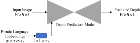
Figure 8: Framework. Depth prediction framework.

Appendix D More Comparisons

In this section, we demonstrate more qualitative comparison in following figures.

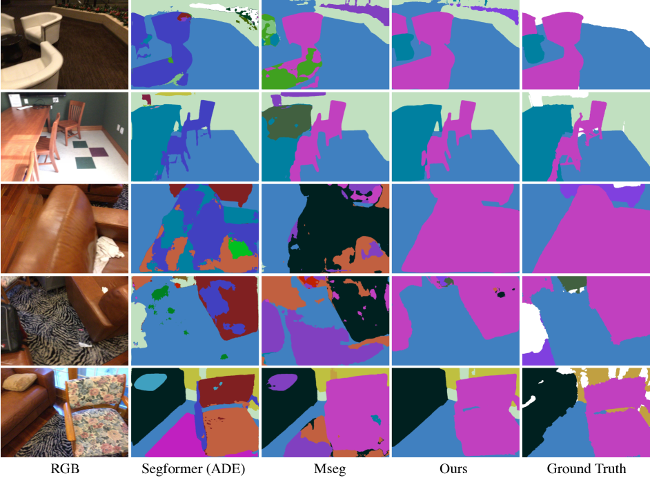
Figure 9: Qualitative Comparisons. We compare with Segformer [56], Mseg [26] on multiple datsets. We employ their released weights for comparison. Note that Segformer model is trained on ADE20K.

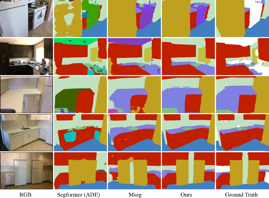
Figure 10: Qualitative Comparisons. We compare with Segformer [56], Mseg [26] on multiple datsets. We employ their released weights for comparison. Note that Segformer model is trained on ADE20K.

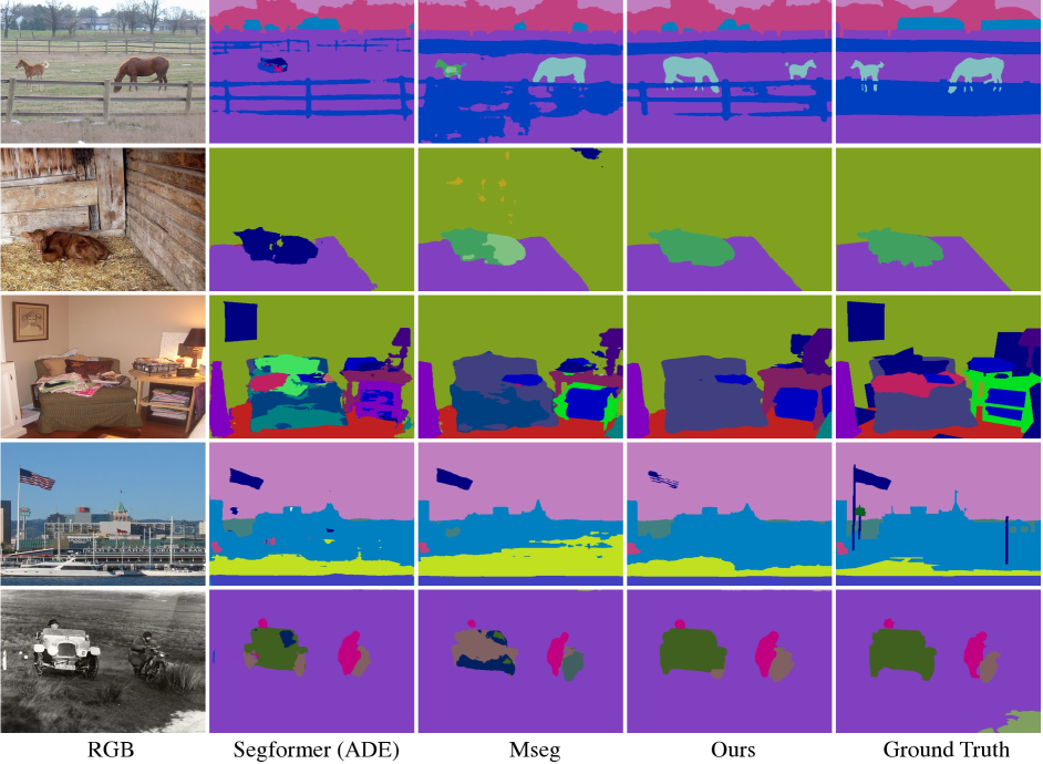
Figure 11: Qualitative Comparisons. We compare with Segformer [56], Mseg [26] on multiple datsets. We employ their released weights for comparison. Note that Segformer model is trained on ADE20K.

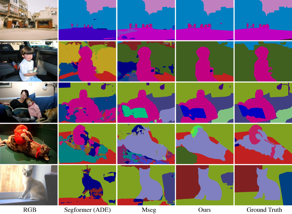
Figure 12: Qualitative Comparisons. We compare with Segformer [56], Mseg [26] on multiple datsets. We employ their released weights for comparison. Note that Segformer model is trained on ADE20K.

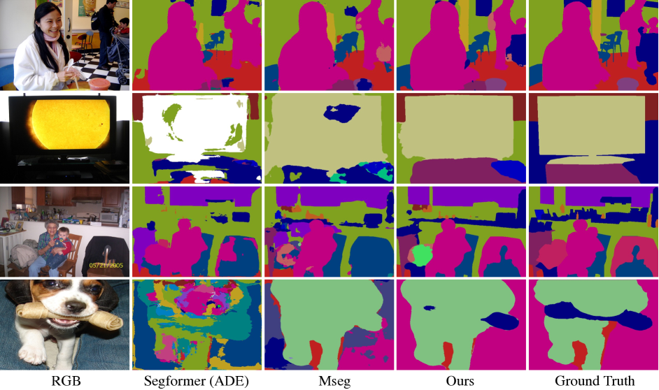
Figure 13: Qualitative Comparisons. We compare with Segformer [56], Mseg [26] on multiple datsets. We employ their released weights for comparison. Note that Segformer model is trained on ADE20K.

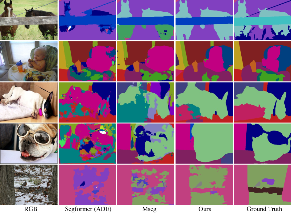
Figure 14: Qualitative Comparisons. We compare with Segformer [56], Mseg [26] on multiple datsets. We employ their released weights for comparison. Note that Segformer model is trained on ADE20K.

References

- [1] Donghyeon Baek, Youngmin Oh, and Bumsub Ham. Exploiting a joint embedding space for generalized zero-shot semantic segmentation. In Int. Conf. Comput. Vis., pages 9536–9545, 2021.
- [2] Rodrigo Benenson, Stefan Popov, and Vittorio Ferrari. Large-scale interactive object segmentation with human annotators. In IEEE Conf. Comput. Vis. Pattern Recog., 2019.
- [3] Petra Bevandić, Ivan Krešo, Marin Oršić, and Siniša Šegvić. Simultaneous semantic segmentation and outlier detection in presence of domain shift. In German Conf. Pattern Recogn., pages 33–47. Springer, 2019.
- [4] Gabriel Brostow, Jamie Shotton, Julien Fauqueur, and Roberto Cipolla. Segmentation and recognition using structure from motion point clouds. In Eur. Conf. Comput. Vis., pages 44–57. Springer, 2008.
- [5] Maxime Bucher, Tuan-Hung Vu, Matthieu Cord, and Patrick Pérez. Zero-shot semantic segmentation. Adv. Neural Inform. Process. Syst., 32:468–479, 2019.
- [6] Sebastian Bujwid and Josephine Sullivan. Large-scale zero-shot image classification from rich and diverse textual descriptions. arXiv: Comp. Res. Repository, 2021.
- [7] Daniel J. Butler, Jonas Wulff, Garrett B. Stanley, and Michael J. Black. A naturalistic open source movie for optical flow evaluation. In Eur. Conf. Comput. Vis., pages 611–625, 2012.
- [8] Jinming Cao, Hanchao Leng, Dani Lischinski, Danny Cohen-Or, Changhe Tu, and Yangyan Li. Shapeconv: Shape-aware convolutional layer for indoor rgb-d semantic segmentation. arXiv: Comp. Res. Repository, page 2108.10528, 2021.
- [9] Siddhartha Chandra, Camille Couprie, and Iasonas Kokkinos. Deep spatio-temporal random fields for efficient video segmentation. In IEEE Conf. Comput. Vis. Pattern Recog., pages 8915–8924, 2018.
- [10] Hao Chen, Kunyang Sun, Zhi Tian, Chunhua Shen, Yongming Huang, and Youliang Yan. BlendMask: Top-down meets bottom-up for instance segmentation. In IEEE Conf. Comput. Vis. Pattern Recog., 2020.
- [11] Weifeng Chen, Shengyi Qian, David Fan, Noriyuki Kojima, Max Hamilton, and Jia Deng. Oasis: A large-scale dataset for single image 3d in the wild. In IEEE Conf. Comput. Vis. Pattern Recog., pages 679–688, 2020.
- [12] Xinlei Chen, Ross Girshick, Kaiming He, and Piotr Dollár. Tensormask: A foundation for dense object segmentation. In Int. Conf. Comput. Vis., pages 2061–2069, 2019.
- [13] Marius Cordts, Mohamed Omran, Sebastian Ramos, Timo Rehfeld, Markus Enzweiler, Rodrigo Benenson, Uwe Franke, Stefan Roth, and Bernt Schiele. The cityscapes dataset for semantic urban scene understanding. In IEEE Conf. Comput. Vis. Pattern Recog., pages 3213–3223, 2016.
- [14] Angela Dai, Angel X Chang, Manolis Savva, Maciej Halber, Thomas Funkhouser, and Matthias Nießner. Scannet: Richly-annotated 3d reconstructions of indoor scenes. In IEEE Conf. Comput. Vis. Pattern Recog., pages 5828–5839, 2017.
- [15] Angela Dai and Matthias Nießner. 3dmv: Joint 3d-multi-view prediction for 3d semantic scene segmentation. In Eur. Conf. Comput. Vis., pages 452–468. Springer, 2018.
- [16] Özgür Erkent and Christian Laugier. Semantic segmentation with unsupervised domain adaptation under varying weather conditions for autonomous vehicles. IEEE Robotics and Automation Letters, 5(2):3580–3587, 2020.
- [17] Mark Everingham, SM Ali Eslami, Luc Van Gool, Christopher KI Williams, John Winn, and Andrew Zisserman. The pascal visual object classes challenge: A retrospective. Int. J. Comput. Vis., 111(1):98–136, 2015.
- [18] Andreas Geiger, Philip Lenz, Christoph Stiller, and Raquel Urtasun. Vision meets robotics: The kitti dataset. Int. J. of Rob. Research, 2013.
- [19] Zhangxuan Gu, Siyuan Zhou, Li Niu, Zihan Zhao, and Liqing Zhang. Context-aware feature generation for zero-shot semantic segmentation. In ACM Int. Conf. Multimedia, pages 1921–1929, 2020.
- [20] Kaiming He, Georgia Gkioxari, Piotr Dollár, and Ross Girshick. Mask r-cnn. In Int. Conf. Comput. Vis., pages 2961–2969, 2017.
- [21] Ping Hu, Stan Sclaroff, and Kate Saenko. Uncertainty-aware learning for zero-shot semantic segmentation. Adv. Neural Inform. Process. Syst., 3:5, 2020.
- [22] Yiwen Hua, Puneet Kohli, Pritish Uplavikar, Anand Ravi, Saravana Gunaseelan, Jason Orozco, and Edward Li. Holopix50k: A large-scale in-the-wild stereo image dataset. In IEEE Conf. Comput. Vis. Pattern Recog. Worksh., June 2020.
- [23] Ye Huang, Wenjing Jia, Xiangjian He, Liu Liu, Yuxin Li, and Dacheng Tao. Channelized axial attention for semantic segmentation. arXiv: Comp. Res. Repository, page 2101.07434, 2021.
- [24] Youngjung Kim, Hyungjoo Jung, Dongbo Min, and Kwanghoon Sohn. Deep monocular depth estimation via integration of global and local predictions. IEEE Trans. Image Process., 27(8):4131–4144, 2018.
- [25] Marvin Klingner, Jan-Aike Termöhlen, Jonas Mikolajczyk, and Tim Fingscheidt. Self-supervised monocular depth estimation: Solving the dynamic object problem by semantic guidance. In Eur. Conf. Comput. Vis., pages 582–600. Springer, 2020.
- [26] John Lambert, Zhuang Liu, Ozan Sener, James Hays, and Vladlen Koltun. MSeg: A composite dataset for multi-domain semantic segmentation. In IEEE Conf. Comput. Vis. Pattern Recog., 2020.
- [27] Zhengqi Li and Noah Snavely. Megadepth: Learning single-view depth prediction from internet photos. In IEEE Conf. Comput. Vis. Pattern Recog., pages 2041–2050, 2018.
- [28] Tsung-Yi Lin, Michael Maire, Serge Belongie, James Hays, Pietro Perona, Deva Ramanan, Piotr Dollár, and C Lawrence Zitnick. Microsoft coco: Common objects in context. In Eur. Conf. Comput. Vis., pages 740–755. Springer, 2014.
- [29] Chenxi Liu, Liang-Chieh Chen, Florian Schroff, Hartwig Adam, Wei Hua, Alan L Yuille, and Li Fei-Fei. Auto-deeplab: Hierarchical neural architecture search for semantic image segmentation. In IEEE Conf. Comput. Vis. Pattern Recog., pages 82–92, 2019.
- [30] Yifan Liu, Chunhua Shen, Changqian Yu, and Jingdong Wang. Efficient semantic video segmentation with per-frame inference. In Eur. Conf. Comput. Vis., pages 352–368. Springer, 2020.
- [31] Ze Liu, Yutong Lin, Yue Cao, Han Hu, Yixuan Wei, Zheng Zhang, Stephen Lin, and Baining Guo. Swin transformer: Hierarchical vision transformer using shifted windows. Int. Conf. Comput. Vis., 2021.
- [32] Jonathan Long, Evan Shelhamer, and Trevor Darrell. Fully convolutional networks for semantic segmentation. In IEEE Conf. Comput. Vis. Pattern Recog., pages 3431–3440, 2015.
- [33] Tomas Mikolov, Ilya Sutskever, Kai Chen, Greg S Corrado, and Jeff Dean. Distributed representations of words and phrases and their compositionality. In Adv. Neural Inform. Process. Syst., pages 3111–3119, 2013.
- [34] George A Miller. Wordnet: a lexical database for english. Communications of the ACM, 38(11):39–41, 1995.
- [35] Roozbeh Mottaghi, Xianjie Chen, Xiaobai Liu, Nam-Gyu Cho, Seong-Whan Lee, Sanja Fidler, Raquel Urtasun, and Alan Yuille. The role of context for object detection and semantic segmentation in the wild. In IEEE Conf. Comput. Vis. Pattern Recog., pages 891–898, 2014.
- [36] Gerhard Neuhold, Tobias Ollmann, Samuel Rota Bulo, and Peter Kontschieder. The mapillary vistas dataset for semantic understanding of street scenes. In Int. Conf. Comput. Vis., pages 4990–4999, 2017.
- [37] Lorenzo Porzi, Samuel Rota Bulò, Aleksander Colovic, and Peter Kontschieder. Seamless scene segmentation. In IEEE Conf. Comput. Vis. Pattern Recog., June 2019.
- [38] Alec Radford, Jong Wook Kim, Chris Hallacy, Aditya Ramesh, Gabriel Goh, Sandhini Agarwal, Girish Sastry, Amanda Askell, Pamela Mishkin, Jack Clark, et al. Learning transferable visual models from natural language supervision. arXiv: Comp. Res. Repository, page 2103.00020, 2021.
- [39] René Ranftl, Alexey Bochkovskiy, and Vladlen Koltun. Vision transformers for dense prediction. In Int. Conf. Comput. Vis., pages 12179–12188, 2021.
- [40] René Ranftl, Katrin Lasinger, David Hafner, Konrad Schindler, and Vladlen Koltun. Towards robust monocular depth estimation: Mixing datasets for zero-shot cross-dataset transfer. IEEE Trans. Pattern Anal. Mach. Intell., 2020.
- [41] German Ros, Simon Stent, Pablo F Alcantarilla, and Tomoki Watanabe. Training constrained deconvolutional networks for road scene semantic segmentation. arXiv: Comp. Res. Repository, page 1604.01545, 2016.
- [42] Shuai Shao, Zeming Li, Tianyuan Zhang, Chao Peng, Gang Yu, Xiangyu Zhang, Jing Li, and Jian Sun. Objects365: A large-scale, high-quality dataset for object detection. In Int. Conf. Comput. Vis., pages 8430–8439, 2019.
- [43] Hengcan Shi, Hongliang Li, Qingbo Wu, and Zichen Song. Scene parsing via integrated classification model and variance-based regularization. In IEEE Conf. Comput. Vis. Pattern Recog., pages 5307–5316, 2019.
- [44] Nathan Silberman, Derek Hoiem, Pushmeet Kohli, and Rob Fergus. Indoor segmentation and support inference from rgbd images. In Eur. Conf. Comput. Vis., pages 746–760. Springer, 2012.
- [45] Shuran Song, Samuel P Lichtenberg, and Jianxiong Xiao. Sun rgb-d: A rgb-d scene understanding benchmark suite. In IEEE Conf. Comput. Vis. Pattern Recog., pages 567–576, 2015.
- [46] Ke Sun, Bin Xiao, Dong Liu, and Jingdong Wang. Deep high-resolution representation learning for human pose estimation. In IEEE Conf. Comput. Vis. Pattern Recog., 2019.
- [47] Zhi Tian, Chunhua Shen, and Hao Chen. Conditional convolutions for instance segmentation. In Eur. Conf. Comput. Vis. Springer, 2020.
- [48] Abhinav Valada, Rohit Mohan, and Wolfram Burgard. Self-supervised model adaptation for multimodal semantic segmentation. Int. J. Comput. Vis., 128(5):1239–1285, 2020.
- [49] Simon Vandenhende, Stamatios Georgoulis, and Luc Van Gool. Mti-net: Multi-scale task interaction networks for multi-task learning. In Eur. Conf. Comput. Vis., pages 527–543. Springer, 2020.
- [50] Girish Varma, Anbumani Subramanian, Anoop Namboodiri, Manmohan Chandraker, and CV Jawahar. Idd: A dataset for exploring problems of autonomous navigation in unconstrained environments. In IEEE Winter Conf. on Applic. of Comp. Vis., pages 1743–1751. IEEE, 2019.
- [51] Igor Vasiljevic, Nick Kolkin, Shanyi Zhang, Ruotian Luo, Haochen Wang, Falcon Z. Dai, Andrea F. Daniele, Mohammadreza Mostajabi, Steven Basart, Matthew R. Walter, and Gregory Shakhnarovich. DIODE: A Dense Indoor and Outdoor DEpth Dataset. arXiv: Comp. Res. Repository, 1908.00463, 2019.
- [52] Xinlong Wang, Rufeng Zhang, Tao Kong, Lei Li, and Chunhua Shen. SOLOv2: Dynamic and fast instance segmentation. In Adv. Neural Inform. Process. Syst., 2020.
- [53] Ke Xian, Jianming Zhang, Oliver Wang, Long Mai, Zhe Lin, and Zhiguo Cao. Structure-guided ranking loss for single image depth prediction. In IEEE Conf. Comput. Vis. Pattern Recog., pages 611–620, 2020.
- [54] Yongqin Xian, Subhabrata Choudhury, Yang He, Bernt Schiele, and Zeynep Akata. Semantic projection network for zero-and few-label semantic segmentation. In IEEE Conf. Comput. Vis. Pattern Recog., pages 8256–8265, 2019.
- [55] Enze Xie, Peize Sun, Xiaoge Song, Wenhai Wang, Xuebo Liu, Ding Liang, Chunhua Shen, and Ping Luo. Polarmask: Single shot instance segmentation with polar representation. In IEEE Conf. Comput. Vis. Pattern Recog., pages 12193–12202, 2020.
- [56] Enze Xie, Wenhai Wang, Zhiding Yu, Anima Anandkumar, Jose M Alvarez, and Ping Luo. SegFormer: Simple and efficient design for semantic segmentation with transformers. Adv. Neural Inform. Process. Syst., 2021.
- [57] Guorun Yang, Hengshuang Zhao, Jianping Shi, Zhidong Deng, and Jiaya Jia. Segstereo: Exploiting semantic information for disparity estimation. In Eur. Conf. Comput. Vis., pages 636–651. Springer, 2018.
- [58] Linjie Yang, Yuchen Fan, and Ning Xu. Video instance segmentation. In Int. Conf. Comput. Vis., pages 5188–5197, 2019.
- [59] Linjie Yang, Yuchen Fan, and Ning Xu. Video instance segmentation. arXiv: Comp. Res. Repository, 1905.04804, 2019.
- [60] Wei Yin, Yifan Liu, and Chunhua Shen. Virtual normal: Enforcing geometric constraints for accurate and robust depth prediction. IEEE Trans. Pattern Anal. Mach. Intell., PP, 2021.
- [61] Wei Yin, Xinlong Wang, Chunhua Shen, Yifan Liu, Zhi Tian, Songcen Xu, Changming Sun, and Dou Renyin. Diversedepth: Affine-invariant depth prediction using diverse data. arXiv: Comp. Res. Repository, page 2002.00569, 2020.
- [62] Wei Yin, Jianming Zhang, Oliver Wang, Simon Niklaus, Long Mai, Simon Chen, and Chunhua Shen. Learning to recover 3d scene shape from a single image. In IEEE Conf. Comput. Vis. Pattern Recog., 2021.
- [63] Fisher Yu, Haofeng Chen, Xin Wang, Wenqi Xian, Yingying Chen, Fangchen Liu, Vashisht Madhavan, and Trevor Darrell. Bdd100k: A diverse driving dataset for heterogeneous multitask learning. In IEEE Conf. Comput. Vis. Pattern Recog., June 2020.
- [64] Yuhui Yuan, Xilin Chen, and Jingdong Wang. Object-contextual representations for semantic segmentation. In Eur. Conf. Comput. Vis., pages 173–190. Springer, 2020.
- [65] Amir Zamir, Alexander Sax, , William Shen, Leonidas Guibas, Jitendra Malik, and Silvio Savarese. Taskonomy: Disentangling task transfer learning. In IEEE Conf. Comput. Vis. Pattern Recog. IEEE, 2018.
- [66] Oliver Zendel, Katrin Honauer, Markus Murschitz, Daniel Steininger, and Gustavo Fernandez Dominguez. Wilddash-creating hazard-aware benchmarks. In Eur. Conf. Comput. Vis., pages 402–416. Springer, 2018.
- [67] Bowen Zhang, Yifan Liu, Zhi Tian, and Chunhua Shen. Dynamic neural representational decoders for high-resolution semantic segmentation. Adv. Neural Inform. Process. Syst., 2021.
- [68] Hang Zhao, Xavier Puig, Bolei Zhou, Sanja Fidler, and Antonio Torralba. Open vocabulary scene parsing. In Int. Conf. Comput. Vis., pages 2002–2010, 2017.
- [69] Hengshuang Zhao, Jianping Shi, Xiaojuan Qi, Xiaogang Wang, and Jiaya Jia. Pyramid scene parsing network. In IEEE Conf. Comput. Vis. Pattern Recog., pages 2881–2890, 2017.
- [70] Bolei Zhou, Hang Zhao, Xavier Puig, Sanja Fidler, Adela Barriuso, and Antonio Torralba. Scene parsing through ade20k dataset. In IEEE Conf. Comput. Vis. Pattern Recog., 2017.
- [71] Yi Zhu, Karan Sapra, Fitsum A Reda, Kevin J Shih, Shawn Newsam, Andrew Tao, and Bryan Catanzaro. Improving semantic segmentation via video propagation and label relaxation. In IEEE Conf. Comput. Vis. Pattern Recog., pages 8856–8865, 2019.