Bayesian inference of the fluctuating proton shape

Abstract

Using Bayesian inference, we determine probabilistic constraints on the parameters describing the fluctuating structure of protons at high energy. We employ the color glass condensate framework supplemented with a model for the spatial structure of the proton, along with experimental data from the ZEUS and H1 Collaborations on coherent and incoherent diffractive $\mathrm{J}/\psi$ production in e+p collisions at HERA. This data is found to constrain most model parameters well. This work sets the stage for future global analyses, including experimental data from e+p, p+p, and p+A collisions, to constrain the fluctuating structure of nucleons along with properties of the final state.

I Introduction

Extracting the multi-dimensional structure of protons and nuclei is one of the main goals of future Deep Inelastic Scattering (DIS) facilities such as the Electron-Ion Collider AbdulKhalek:2021gbh ; Aschenauer:2017jsk , LHeC/FC-he Agostini:2020fmq and EicC Anderle:2021wcy . Exclusive processes like $\mathrm{J}/\psi$ production are especially powerful probes of the hadron structure at a small longitudinal momentum fraction $x$ for two reasons. First, the exclusive nature of the process requires at lowest order at least two gluons to be exchanged with the target, rendering the cross section approximately proportional to the squared gluon distribution Ryskin:1992ui . Additionally, only in exclusive processes is it possible to measure the total momentum transfer, which is Fourier conjugate to the impact parameter and thereby provides access to the transverse geometry.

Understanding the proton structure, including its event-by-event fluctuations Mantysaari:2020axf , is of fundamental interest. Additionally, knowledge of the spatial structure of the colliding objects in hadronic and heavy-ion collisions is required in order to construct realistic initial conditions that can be coupled to relativistic hydrodynamic simulations to describe the space-time evolution of the produced Quark-Gluon Plasma (QGP). Besides heavy-ion collisions, collective phenomena that can be interpreted as signatures of QGP production have been seen in small systems such as proton/deuteron/³He - nucleus ALICE:2012eyl ; CMS:2012qk ; ATLAS:2012cix ; PHENIX:2018lia ; STAR:2019zaf , proton-proton CMS:2010ifv , and even photon-nucleus collisions ATLAS:2021jhn , see Dusling:2015gta ; Loizides:2016tew ; Schlichting:2016sqo ; Nagle:2018nvi ; Schenke:2019pmk ; Schenke:2021mxx for reviews. In such small collision systems with a proton projectile, the detailed fluctuation spectrum of the proton geometry is particularly important to determine if QGP is indeed produced.

It is possible to constrain the proton structure from hadronic collisions by performing a statistical analysis to extract both the transport coefficients describing the matter produced in proton-lead collisions (see e.g. Refs. JETSCAPE:2021ehl ; JETSCAPE:2020mzn ; JETSCAPE:2020shq ; Bernhard:2019bmu ; Bernhard:2016tnd ; Parkkila:2021yha ; Parkkila:2021tqq ), as well as the proton’s fluctuating geometry, by comparing with the LHC data as in Ref. Moreland:2018gsh . Another approach, which we take in this work, is to use exclusive DIS data from HERA, especially exclusive vector meson production H1:2013okq ; Aktas:2005xu ; Chekanov:2002xi ; Chekanov:2002rm ; Aktas:2003zi , as a complementary input to constrain the proton shape fluctuations, as initially suggested in Ref. Mantysaari:2016ykx . In the future, the Electron-Ion Collider will provide a vast amount of precise vector meson production data with proton and nuclear targets that will provide further constraints on e.g. momentum fraction $x_{\mathbb{P}}$ and the nuclear mass number $A$ dependence. Additionally, Ultra Peripheral Collisions Klein:2019qfb ; Bertulani:2005ru at RHIC PHENIX:2009xtn and at the LHC ALICE:2014eof ; ALICE:2018oyo ; LHCb:2014acg ; LHCb:2018rcm ; CMS:2016itn ; ALICE:2021tyx provide access to very high energy photoproduction processes and to effects of a nuclear environment on nucleon substructure fluctuations at high energy Mantysaari:2017dwh ; Sambasivam:2019gdd .

In this work, we go beyond previous studies Mantysaari:2016ykx ; Mantysaari:2016jaz , where model parameters were constrained “by eye”, and perform a Bayesian analysis to extract in a statistically rigorous manner the non-perturbative parameter values allowed by the HERA data, and construct initial conditions for hadronic collisions that are compatible with the experimental DIS data.

This paper is organized as follows. In Section II we review the calculation of coherent and incoherent exclusive vector meson production in the dipole picture and discuss the various aspects of our model for the proton target. In Section III we explain the procedure for our Bayesian analysis. We present results in Section IV and conclude in Section V.

II Vector meson production at high energy

In this work we calculate vector meson production in a framework similar to the one used in Refs. Mantysaari:2016jaz ; Mantysaari:2016ykx (see also Refs. Kumar:2021zbn ; Cepila:2018zky ; Traini:2018hxd ; Cepila:2017nef ; Cepila:2016uku ), and for completeness briefly review the calculation in this section.

At high energies, DIS processes can be conveniently described in the dipole picture in the rest frame of the target proton, and interaction with the target color field is described in the Color Glass Condensate (CGC) framework Kovchegov:2012mbw ; Iancu:2003xm ; Gelis:2010nm ; Albacete:2014fwa . In the proton rest frame, the lifetime of a fluctuation of the incoming virtual photon into a quark-antiquark dipole is much longer than the characteristic timescale of the dipole-target interaction. Consequently, the scattering amplitude can be factorized into a convolution of photon and vector meson wave functions and the dipole-target interaction. The scattering amplitude for exclusive vector meson $V$ production can then be written as Kowalski:2006hc ; Hatta:2017cte

$$\mathcal{A}^{\gamma^{*}+p\to V+p}=2i\int\differential[2]{{\mathbf{r}_{\perp}}}\differential[2]{{\mathbf{b}_{\perp}}}\frac{\differential{z}}{4\pi}e^{-i\left[{\mathbf{b}_{\perp}}-\left(\frac{1}{2}-z\right){\mathbf{r}_{\perp}}\right]\cdot{\boldsymbol{\Delta}_{\perp}}}\\ \times[\Psi_{V}^{*}\Psi_{\gamma}](Q^{2},{\mathbf{r}_{\perp}},z)N_{\Omega}({\mathbf{r}_{\perp}},{\mathbf{b}_{\perp}},x_{\mathbb{P}}).$$ (1)

Here ${\mathbf{r}_{\perp}}$ is the transverse size of the $q\bar{q}$ dipole, ${\mathbf{b}_{\perp}}$ is the impact parameter measured relative to the proton center, and $Q^{2}$ is the photon virtuality. The fraction of the large photon plus momentum carried by the quark is given by $z$, and ${\boldsymbol{\Delta}_{\perp}}$ is the transverse momentum transfer. Note that at high energies we can employ the eikonal approximation and assume that the quark transverse coordinates are fixed during the propagation through the target color field.

The $\gamma^{*}\to q\bar{q}$ splitting is described by the virtual photon light front wave function $\Psi_{\gamma}$, which can be computed from QED Kovchegov:2012mbw . The vector meson wave function is non-perturbative, and in this work, we use the so-called Boosted Gaussian parametrization from Kowalski:2006hc , where the model parameters are constrained by experimental data on the vector meson decay width. We note that there are multiple vector meson wave functions proposed in the literature (see e.g. Refs. Lappi:2020ufv ; Li:2017mlw ; Li:2021cwv ). Different wave functions mostly affect the overall normalization of the $\mathrm{J}/\psi$ production cross section, and have a much smaller effect on the $|t|$ spectra, which we are most interested here Lappi:2020ufv ; Mantysaari:2017dwh ; Kowalski:2006hc . Consequently, our results will depend only weakly on the specific wave function choice (except for the parameter controlling the overall proton density).

Equation (1) is a leading order result for the vector meson production in the CGC framework (note that multiple scattering effects are resummed in the dipole amplitude $N_{\Omega}$). Currently, there is rapid progress in the field toward next-to-leading order (NLO) accuracy. In particular, the cross section for the production of light mesons Boussarie:2016bkq and longitudinally polarized heavy vector mesons are now available Mantysaari:2021ryb at next-to-leading order, as well as the virtual photon light front wave function Beuf:2021srj ; Beuf:2020dxl ; Beuf:2021qqa ; Hanninen:2017ddy ; Beuf:2017bpd ; Beuf:2016wdz and small-$x$ evolution equations Lappi:2020srm ; Lappi:2016fmu ; Lappi:2015fma ; Balitsky:2008zza ; Ducloue:2019ezk ; Ducloue:2019jmy ; Iancu:2015vea ; Iancu:2015joa ; Balitsky:2013fea ; Kovner:2013ona (see also Ref. Caucal:2021ent where dijet production is studied at next-to-leading order). However, the NLO calculations are not yet at the level where they can be consistently used in phenomenological applications (in particular the cross section for transversely polarized heavy vector meson production is still missing). As the purpose of this work is to demonstrate the potential of Bayesian analyses to systematically extract non-perturbative parameters describing the proton event-by-event fluctuating structure, we do not expect the NLO contributions to have a large effect on the results we obtain using our leading order setup.

The coherent cross section, corresponding to the process where the target proton remains in the same quantum state, can be obtained by averaging over the target color charge configurations $\Omega$ at the amplitude level Good:1960ba :

$$\frac{\differential\sigma^{\gamma^{*}+p\to V+p}}{\differential|t|}=\frac{1}{16\pi}\left|\left\langle\mathcal{A}^{\gamma^{*}+p\to V+p}\right\rangle_{\Omega}\right|^{2}$$ (2)

Subtracting the coherent contribution from the total diffractive vector meson production cross section we obtain the cross section for incoherent vector meson production, in which case the final state of the target is different from the initial state Miettinen:1978jb ; Caldwell:2010zza ; Mantysaari:2020axf . Experimentally, this corresponds to processes where the target proton (or nucleus) dissociates, but the rapidity gap between the produced vector meson and the target remnants remains. The incoherent cross section can then be written as a variance

$$\frac{\differential\sigma^{\gamma^{*}+p\to V+p^{*}}}{\differential|t|}=\frac{1}{16\pi}\left[\left\langle\left|\mathcal{A}^{\gamma^{*}+p\to V+p}\right|^{2}\right\rangle_{\Omega}\right.\\ -\left.\left|\left\langle\mathcal{A}^{\gamma^{*}+p\to V+p}\right\rangle_{\Omega}\right|^{2}\right]\,.$$ (3)

Dependence on the small-$x$ structure of the target proton is included in the dipole amplitude $N_{\Omega}({\mathbf{r}_{\perp}},{\mathbf{b}_{\perp}},x_{\mathbb{P}})$, which, for a given target color charge configuration $\Omega$, can be written as

$$N_{\Omega}({\mathbf{r}_{\perp}},{\mathbf{b}_{\perp}},x_{\mathbb{P}})=1-\frac{1}{{N_{\mathrm{c}}}}\tr\left[V\left({\mathbf{b}_{\perp}}+\frac{{\mathbf{r}_{\perp}}}{2}\right)V^{\dagger}\left({\mathbf{b}_{\perp}}-\frac{{\mathbf{r}_{\perp}}}{2}\right)\right].$$ (4)

Here $V({\mathbf{x}_{\perp}})$ represents a Wilson line, which describes the color rotation of a quark state when it propagates through the target field (given the target color field configuration $\Omega$) at transverse coordinate ${\mathbf{x}_{\perp}}$. We suppressed the dependence of $V$ on

$$x_{\mathbb{P}}\approx\frac{M_{V}^{2}+Q^{2}}{W^{2}+Q^{2}}\,,$$ (5)

which is the fraction of the target longitudinal momentum transferred to the meson with mass $M_{V}$ in the frame where the target has a large momentum. We neglect the $t$ dependence of $x_{\mathbb{P}}$ in this work. The photon-proton center-of-mass energy is denoted by $W$.

The Wilson lines are obtained in the same way as done in the IP-Glasma calculation Schenke:2012wb used e.g. in Refs. Mantysaari:2020lhf ; Mantysaari:2019jhh ; Mantysaari:2019csc ; Mantysaari:2018zdd ; Mantysaari:2016jaz ; Mantysaari:2016ykx . The color charges $\rho^{a}$ are first determined using the McLerran-Venugopalan McLerran:1993ni model, assuming that color charges are local Gaussian random variables with expectation value zero and variance

$$g^{2}\left\langle\rho^{a}(x^{-},{\mathbf{x}_{\perp}})\rho^{b}(y^{-},{\mathbf{y}_{\perp}})\right\rangle=g^{4}\lambda_{A}(x^{-})\delta^{ab}\\ \times\delta^{(2)}({\mathbf{x}_{\perp}}-{\mathbf{y}_{\perp}})\delta(x^{-}-y^{-})\,.$$ (6)

Here the color charge density is $\mu^{2}=\int\differential{x^{-}}\lambda_{A}(x^{-})$, and it is related to the local saturation scale $Q_{s}({\mathbf{x}_{\perp}})$ determined from the IPsat parametrization Kowalski:2003hm fitted to HERA data Rezaeian:2012ji ; Mantysaari:2018nng . In our Bayesian analysis, the ratio

$$\frac{Q_{s}({\mathbf{x}_{\perp}})}{g^{2}\mu}\,,$$ (7)

is a free parameter, controlling the overall proton density (see also Ref. Lappi:2007ku for a detailed study of this ratio). The Wilson lines $V({\mathbf{x}_{\perp}})$ can be obtained by solving the Yang-Mills equations, and the result reads

$$V({\mathbf{x}_{\perp}})=\mathrm{P}_{-}\left\{\exp\left({-ig\int_{-\infty}^{\infty}\differential{z^{-}}\frac{\rho^{a}(x^{-},{\mathbf{x}_{\perp}})t^{a}}{\boldsymbol{\nabla}^{2}-m^{2}}}\right)\right\}\,,$$ (8)

where $P_{-}$ represents path ordering in the $x^{-}$ direction. Here, we introduced the infrared regulator $m$, which is needed to avoid the emergence of unphysical Coulomb tails, and will be another free parameter in the Bayesian analysis.

In the IPsat parametrization the saturation scale $Q_{s}^{2}({\mathbf{b}_{\perp}})$ is directly proportional to the local density $T_{p}({\mathbf{b}_{\perp}})$. We introduce an event-by-event fluctuating density by writing the density profile following Refs. Mantysaari:2016jaz ; Mantysaari:2016ykx as:

$$T_{p}({\mathbf{b}_{\perp}})=\frac{1}{N_{q}}\sum_{i=1}^{N_{q}}p_{i}T_{q}({\mathbf{b}_{\perp}}-{\mathbf{b}_{\perp,i}}),$$ (9)

where

$$T_{q}({\mathbf{b}_{\perp}})=\frac{1}{2\pi B_{q}}e^{-{\mathbf{b}}_{\perp}^{2}/(2B_{q})}\,,$$ (10)

and the coefficient $p_{i}$ allows for different normalizations for individual hot spots, to be discussed below. Our prescription corresponds to having $N_{q}$ hot spots with hot spot width $B_{q}$ (note that the hot spot transverse root mean square (RMS) radius in $\sqrt{2B_{q}}$). The hot spot positions ${\mathbf{b}_{\perp,i}}$ are sampled from a two-dimensional Gaussian distribution whose width is denoted by $B_{qc}$, and the center-of-mass is shifted to the origin in the end.

As discussed in Ref. Albacete:2016pmp ; Albacete:2017ajt , repulsive short-range correlations between the hot spots may explain the hollowness effect Alkin:2014rfa ; Dremin:2015ujt ; Troshin:2016frs ; Arriola:2016bxa and negative correlation between the $v_{2}$ and $v_{3}$ flow harmonics observed in highest multiplicity proton-proton collisions Sirunyan:2017uyl ; Acharya:2019vdf . In order to study if exclusive vector meson production in DIS can be used to probe such repulsive correlations, we also introduce an additional model parameter $d_{q,\text{Min}}$ which controls the minimum three-dimensional distance required between any two hot spots. We checked that for a large number of hot spots $N_{q}=10$ in a typical nucleon of size $B_{qc}=4.2$ GeV^-2, the model parameter $d_{q,\mathrm{Min}}$ remains effective more than 90% for $d_{q,\mathrm{Min}}\leq 0.4$ fm, meaning that in 10% of the sampled configurations the distance requirement cannot be fulfilled.

Finally, we include saturation scale fluctuations by allowing the local density of each hot spot to fluctuate independently, following again Refs. Mantysaari:2016jaz ; Mantysaari:2016ykx (see also Ref. McLerran:2015qxa ). These fluctuations are implemented by sampling the coefficients $p_{i}$ in Eq. (9) from the log-normal distribution

$$P\left(\ln p_{i}\right)=\frac{1}{\sqrt{2\pi}\sigma}\exp\left[-\frac{\ln^{2}p_{i}}{2\sigma^{2}}\right]\,.$$ (11)

The sampled $p_{i}$ are at the end normalized by the expectation value of the distribution $E[p_{i}]=e^{\sigma^{2}/2}$ in order to keep the average density unmodified. The magnitude of density fluctuations is controlled by the parameter $\sigma$.

III Bayesian analysis setup

Bayesian Inference is a general and systematic method to constrain the probability distribution of model parameters ${\boldsymbol{\theta}}$ by comparing model calculations $\mathbf{y}({\boldsymbol{\theta}})$ with experimental measurements $\mathbf{y}_{\mathrm{exp}}$ sivia2006data . Bayes’ theorem provides the posterior distribution of model parameters as

$${\mathcal{P}}({\boldsymbol{\theta}}|\mathbf{y}_{\mathrm{exp}})\propto{\mathcal{P}}(\mathbf{y}_{\mathrm{exp}}|{\boldsymbol{\theta}}){\mathcal{P}}({\boldsymbol{\theta}}).$$ (12)

Here ${\mathcal{P}}(\mathbf{y}_{\mathrm{exp}}|{\boldsymbol{\theta}})$ is the likelihood for model results with parameter ${\boldsymbol{\theta}}$ to agree with the experimental data. We choose a multivariate normal distribution for the logarithm of the likelihood with $\Delta\mathbf{y}({\boldsymbol{\theta}})=\mathbf{y}({\boldsymbol{\theta}})-\mathbf{y}_{\mathrm{exp}}$ williams2006gaussian ,

$$\ln[{\mathcal{P}}(\mathbf{y}_{\mathrm{exp}}|{\boldsymbol{\theta}})] = -\frac{1}{2}\Delta\mathbf{y}({\boldsymbol{\theta}})^{T}\Sigma^{-1}\Delta\mathbf{y}({\boldsymbol{\theta}})$$ (13)

$$-\frac{1}{2}\ln[(2\pi)^{n}\det\Sigma].$$

Here $n$ is the number of experimental data points and $\Sigma\equiv\Sigma_{\mathrm{exp}}+\Sigma_{\mathrm{model}}$ is the $n\times n$ covariance matrix, which encodes experimental and model uncertainties. In the current analysis, we assume no correlation among experimental errors of the $n$ observables $\{\sigma_{i}\}$. So the covariance matrix for experimental uncertainty takes a diagonal form,

$$\Sigma_{\mathrm{exp}}=\mathrm{diag}(\sigma_{1}^{2},\cdots,\sigma_{n}^{2}).$$ (14)

Our model uncertainties $\Sigma_{\mathrm{model}}$ are estimated using the covariance matrix from the trained Gaussian Process (GP) Emulators Bernhard:2015hxa .

Table 1: Summary of model parameters, their prior ranges, and constrained maximum likelihood values with uncertainty estimates in 90% credible intervals.

Parameter	Description	Prior range	MAP (variable $N_{q}$)	MAP ($N_{q}\equiv 3$)
$m$ $[\mathrm{GeV}]$	Infrared regulator	[0.05, 2]	$0.506^{+1.12}_{-0.356}$	$0.246^{+0.162}_{-0.103}$
$B_{qc}$ $[\mathrm{GeV}^{-2}]$	Proton size	[1, 10]	$4.02^{+1.73}_{-0.728}$	$4.45^{+0.801}_{-0.803}$
$B_{q}$ $[\mathrm{GeV}^{-2}]$	Hot spot size	[0.1, 3]	$0.474^{+0.434}_{-0.286}$	$0.346^{+0.282}_{-0.202}$
$\sigma$	Magnitude of $Q_{s}$ fluctuations	[0, 1.5]	$0.833^{+0.194}_{-0.441}$	$0.563^{+0.143}_{-0.141}$
$Q_{s}/(g^{2}\mu)$	Ratio of color charge density and saturation scale	[0.2, 1.5]	$0.598^{+0.230}_{-0.264}$	$0.747^{+0.0704}_{-0.0930}$
$d_{q,\text{Min}}$ $[\mathrm{fm}]$	Minimum 3D distance between hot spots	[0, 0.5]	$0.257^{+0.221}_{-0.231}$	$0.254^{+0.222}_{-0.229}$
$N_{q}$	Number of hot spots	[1, 10]	$6.79^{+2.93}_{-4.83}$	$3$

We employ GP emulators williams2006gaussian for our model and couple them with the Monte-Carlo Markov Chain (MCMC) method to efficiently explore the model parameter space goodman2010ensemble ; foreman2013emcee . The HERA measurements can be represented by five Principal Components (PC) with a residual variance of less than 0.01%, meaning that 99.99% of the variation of all studied observables within the prior parameter range are captured by the five principal components. Our GP emulators are trained to fit these five PCs with 1,000 training simulations in the model parameter space. In each model parameter point, we generate 3,000 configurations to compute the coherent and incoherent cross sections. The relative statistical errors are within 5%.

All model parameters and their prior ranges (and Maximum a Posterior values that are discussed in Sec. IV) are summarized in Table. 1. We treat the parameter $N_{q}$ as a continuous real number. The fractional part of $N_{q}$ is treated as a probability to sample either $\lceil N_{q}\rceil$ or $\lfloor N_{q}\rfloor$ partons inside protons. The same approach was recently used in Ref. Nijs:2021clz . The experimental data included in the Bayesian analysis is the H1 data on coherent and incoherent $\mathrm{J}/\psi$ production cross section measured at $W=75\,\mathrm{GeV}$ H1:2013okq . The incoherent data is included in the $|t|$ range $0<|t|<2.5$ $\mathrm{GeV}^{2}$. We note that there is incoherent data at higher $|t|$ also (studied in a similar context in Ref. Kumar:2021zbn ), but the highest $|t|$ points are not included in our analysis for two reasons. First, as we determine Wilson lines at fixed $x_{\mathbb{P}}$, as discussed in Sec. II, and do not include the full $x_{\mathbb{P}}$ evolution, we neglect $|t|$ dependence in $x_{\mathbb{P}}$ (see Eq. (5)). Additionally, at large $|t|$ other effects such as DGLAP evolution Gribov:1972ri ; Gribov:1972rt ; Altarelli:1977zs ; Dokshitzer:1977sg may become important.

IV Results

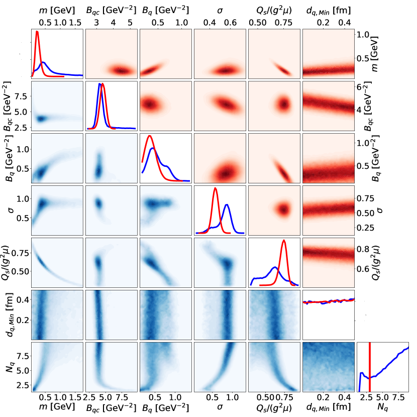
Figure 1: Bayesian posterior distributions of the model parameters. The diagonal panels show the probability distributions for individual parameters, and off-diagonal panels illustrate their pairwise correlations.

For two distinct scenarios, the first with $N_{q}$ fixed to 3, the second with $N_{q}$ a free parameter, the posterior distribution of model parameters is shown in Fig. 1. Particularly for the case of $N_{q}=3$, most of the model parameters are tightly constrained by the H1 data included in the Bayesian analysis. This is due to the fact that different regions of the dataset are sensitive to different model parameters.

First, the infrared regulator $m$ suppresses long-distance Coulomb tails, and as such, it controls the shape of the proton at large distances. This part of the proton geometry is probed by coherent diffraction at low $|t|\lesssim 0.2\mathrm{GeV}^{2}$ Mantysaari:2016jaz : impact parameter and momentum transfers are Fourier conjugates, and consequently the low-$|t|$ region is sensitive to large distances and vice versa. On the other hand, the actual proton size controlled mostly by $B_{qc}$ determines the overall slope of the coherent spectrum. The hot spot size $B_{q}$ then determines the slope of the incoherent cross section in the $|t|\gtrsim 1\,\mathrm{GeV}^{2}$ region: as shown in Ref. Lappi:2010dd the slope of the incoherent spectra at high $|t|$ is given by the size of the smallest fluctuating constituent.

The overall normalization is determined by the $Q_{s}/(g^{2}\mu)$ parameter and the magnitude of the cross sections constrains that, however, it can not be determined very precisely from our analysis as it is strongly correlated with many other parameters, particularly for the case that $N_{q}$ is a free parameter. Here we note that there is some model uncertainty related to the non-perturbative vector meson wave functions, and different phenomenological parametrizations can result in cross sections that differ by $\sim 20\%$, see e.g. Lappi:2020ufv ; Mantysaari:2017dwh ; Kowalski:2006hc . In phenomenological analyses, the so-called skewness correction Kowalski:2006hc is sometimes included, which can also have a numerically significant (up to $\sim 40\%$) effect on the cross section. However, as there are also other model uncertainties related to the overall normalization and the applicability of the skewness correction in our setup is not rigorously justified, it is not included in this work. The small real part correction discussed e.g. in Ref. Kowalski:2006hc is also neglected.

One can see that when leaving $N_{q}$ variable, its value can not be constrained in our analysis, except that $N_{q}\geq 2$ is required in order to get geometry fluctuations that are necessary to describe the incoherent HERA data. At first one would expect the configurations with large $N_{q}$ to be so smooth that event-by-event fluctuations would not be enough to result in a large enough incoherent cross section. However, we note that there is a strong positive correlation between $N_{q}$ and $\sigma$, which means that large $N_{q}$ goes along with large hot spot density fluctuations. In this situation one can not really interpret $N_{q}$ as the number of hot spots, but one has to consider effective hot spots, that are generated dynamically from the sum of the $N_{q}$ constituents that are each strongly fluctuating in magnitude. This effective hot spot number will generally be smaller than $N_{q}$. For a quantitative analysis a hot spot finding prescription, similar to jet clustering algorithms, would be needed. Additional constraints for $\sigma$ originate from the incoherent cross section at small $|t|$, which is sensitive to the fluctuations at long-distance scales, i.e., overall density fluctuations Mantysaari:2016jaz ; Mantysaari:2016ykx .

The minimum distance required between the hot spots in three dimensions, $d_{q,\text{Min}}$, can not be constrained at all in our analysis. This parameter is also only very weakly correlated with the other parameters, emphasizing its limited effect on the results. This means that the $\mathrm{J}/\psi$ production data allows, but does not require, repulsive short-range correlations used e.g. in Refs. Albacete:2016pmp ; Albacete:2017ajt . We note that for large $N_{q}$ it is not always possible to fulfill the minimum distance requirement, reducing the effective value of $d_{q,{\rm Min}}$ that is actually employed.

Let us next study correlations between the model parameters in more detail. First, we observe that there is a clear positive correlation between the infrared regulator $m$ and the hot spot size $B_{q}$. This can be understood, as increasing $m$ suppresses color fields at large distances and as such results in smaller hot spots. Interestingly, we find no clear correlation between the overall proton size parameter $B_{qc}$ and the infrared regulator $m$. In fact, the proton size $B_{qc}$ shows no clear correlation with any of the other model parameters. The infrared regulator $m$ is strongly anti-correlated with $Q_{s}/(g^{2}\mu)$. This is again easy to understand: large $m$ results in a reduction of the normalization of the cross section, which has to be compensated by using a larger color charge density which requires smaller $Q_{s}/(g^{2}\mu)$.

We also find a strong negative correlation between the number of hot spots $N_{q}$ and the proton density $Q_{s}/(g^{2}\mu)$. This correlation can be understood by considering the effect of these parameters on the incoherent cross section. When the number of hot spots with the same size increases, the incoherent slope is not significantly affected but the normalization goes down as there are smaller fluctuations in the scattering amplitude due to the smoother proton profile. This would result in the incoherent cross section being underestimated, which has to be compensated by smaller $Q_{s}/(g^{2}\mu)$.

The somewhat surprising negative correlation between the hot spot size $B_{q}$ and the proton density $Q_{s}/(g^{2}\mu)$ can also be understood. First, we note that large hot spots (large $B_{q}$) require a larger infrared regulator $m$ which effectively makes the hot spots smaller (notice a positive correlation between $B_{q}$ and $m$). Then, to compensate for the effect of the larger infrared regulator on the magnitude of the cross section, a smaller $Q_{s}/(g^{2}\mu)$ is needed.

The posterior distribution of parameters $B_{qc}$ and $B_{q}$, that determine the proton size, which can be quantified e.g. by the two dimensional RMS radius, $r_{\rm rms}=\sqrt{2(B_{\rm qc}+B_{q})}$, are shown in the second and third diagonal panels of Fig. 1. We find that they are sharply peaked, in particular for the case of fixed $N_{q}=3$. The extracted proton radius from this Bayesian analysis is $r_{\rm rms}=0.591^{+0.130}_{-0.071}\,{\rm fm}$ ($0.610^{+0.065}_{-0.068}\,{\rm fm}$) for variable $N_{q}$ ($N_{q}\equiv 3$) with uncertainty estimates in 90% credible intervals.

We further included the possibility of fluctuating values of $B_{q}$ and $N_{q}$, and studied the dependence of the observables on the respective variances. We found that the considered experimental data could not constrain these parameters and decided not to include them in the presented analysis.

Next, we demonstrate explicitly that sampling parameter values from the posterior distribution lead to a good description of the HERA data. The main result of the Bayesian analysis is the posterior distribution shown in Fig. 1, but it is also possible to find the so-called Maximum a Posteriori (MAP) parameter set, which is the mode of the posterior distribution. Because our prior parameter distributions are uniform, the MAP parameters shown in Table 1 maximize the likelihood function and provide the best fit to the experimental data. We note that statistically the expectation value for any observable is not obtained using the MAP parameters. Instead, one should calculate observables using averages over parameter samples obtained from the posterior distribution.

Comparison to the HERA coherent and incoherent $\mathrm{J}/\psi$ production data measured at $W=75\,\mathrm{GeV}$ H1:2013okq and used in the Bayesian analysis to constrain the model parameters are shown in panel (a) of Fig. 2. The spectra calculated by averaging the results computed using different parametrizations sampled from the posterior distribution indeed provide an excellent description of the data. We also show the statistical uncertainty, obtained by calculating the one standard deviation interval shown as red (coherent) and blue (incoherent) bands.

Next, we study compatibility with experimental data not included in the Bayesian analysis. We do not include full small-$x$ evolution e.g. by means of the JIMWLK Jalilian-Marian:1996mkd ; Jalilian-Marian:1997qno ; Jalilian-Marian:1997jhx ; Iancu:2001md ; Ferreiro:2001qy ; Iancu:2001ad ; Iancu:2000hn ; Mueller:2001uk equation in this work. Consequently, the only center-of-mass energy $W$ (or momentum fraction $x_{\mathbb{P}}$) dependence comes from the $x_{\mathbb{P}}$ dependence of the saturation scale $Q_{s}$ determined from the IPsat fit. This almost only affects the overall normalization of the calculated spectra, and misses important physical effects such as the growth of the proton with decreasing $x$. Consequently, we do not expect that within our setup we can describe $\mathrm{J}/\psi$ production at different center-of-mass energies simultaneously. Nevertheless, the geometry evolution between $W=75\,{\rm GeV}$ and $W=100\,{\rm GeV}$ should be weak enough to make predictions for the higher center-of-mass energy.

The calculated $\mathrm{J}/\psi$ spectra at $W=100\,{\rm GeV}$ are shown in panel (b) of Fig. 2 and compared with the data from H1 and ZEUS collaborations Aktas:2005xu ; ZEUS:2002wfj ; Chekanov:2002rm ; Aktas:2003zi . Again, we show the model prediction as the average over many samples of the posterior distribution and provide one standard deviation bands. The results are very similar to the $W=75\,\mathrm{GeV}$ case studied above, and the HERA data is well described (except the coherent cross section at low $|t|$, and high $|t|$ in the case of the ZEUS measurement), and variation between the different parametrizations sampled from the posterior distribution is small. Similarity to the $W=75\,\mathrm{GeV}$ case is not surprising, as we use exactly the same fluctuating geometry, with the only difference being slightly larger $Q_{s}$ values, extracted from the IPsat parametrization.

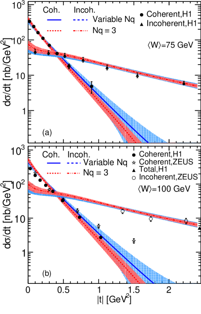
Figure 2: Coherent and incoherent $\mathrm{J}/\psi$ photoproduction cross sections at $\langle W\rangle=75\,\mathrm{GeV}$ (a) and $\langle W\rangle=100\,\mathrm{GeV}$ (b), calculated by averaging over many parameter sets sampled from the posterior distribution, which was determined using the $\langle W\rangle=75\,\mathrm{GeV}$ HERA data H1:2013okq . We compare the case with variable $N_{q}$ to that with fixed $N_{q}=3$, and to experimental data at $\langle W\rangle=75\,\mathrm{GeV}$ H1:2013okq and $\langle W\rangle=100\,\mathrm{GeV}$ Aktas:2005xu ; Chekanov:2002xi ; Chekanov:2002rm ; Aktas:2003zi , respectively. The bands show the one standard deviation uncertainty.

V Conclusions

We have performed a statistically rigorous Bayesian analysis to extract posterior likelihood distributions for the non-perturbative parameters describing the event-by-event fluctuating proton geometry as constrained by exclusive $\mathrm{J}/\psi$ production data from HERA. We presented a comparison of the $|t|$-dependent coherent and incoherent cross sections, obtained from an average over many parameter samples from the posterior distribution, to the experimental data.

Generally, model parametrizations sampled from the determined posterior distribution can be used to systematically take into account uncertainties in the proton geometry as constrained by the HERA DIS data when calculating any other observable that depends on the proton geometry, such as flow observables in high-multiplicity proton-proton and proton-nucleus collisions. To enable such studies, we provide 1,000 parametrizations sampled from the determined posterior distributions in the supplemental material.

Because the model parameters are sensitive to different aspects of the coherent and incoherent vector meson production spectra, most of them are well constrained by the Bayesian analysis. The only exceptions are the minimum distance between the hot spots (repulsive short-range correlations), and the number of hot spots $N_{q}$, which cannot be well constrained by the considered HERA data. However, we note that although the analysis suggests that large $N_{q}$ is compatible with the HERA data, for $N_{q}\gtrsim 5$ one should no longer simply interpret $N_{q}$ as the number of actual hot spots. In this regime, a good description of the data requires large fluctuations of individual hot spots’ densities, and the sampled ‘hot spots’ can also overlap significantly. Thus, the effective number of hot spots is significantly smaller than the parameter $N_{q}$ might imply.

The HERA data used in this work probes the proton structure at $x\sim 10^{-3}$. The energy (Bjorken-$x$) dependence can be included in terms of JIMWLK evolution as e.g. in Refs. Schlichting:2014ipa ; Mantysaari:2018zdd . In the future we plan to extend our framework by including the full JIMWLK evolution and vector meson production data at different center-of-mass energies from HERA ZEUS:2002wfj ; H1:2013okq ; H1:2005dtp ; H1:2013okq and from the ultra peripheral proton-lead collisions measured at the LHC Aaij:2014iea ; Acharya:2018jua ; LHCb:2014acg ; LHCb:2018rcm , allowing us to extract also the Bjorken-$x$ dependence of the fluctuating proton geometry.

In addition to constraining the energy dependence, performing global analyses including both exclusive vector meson production data from HERA and flow harmonics from the proton-proton and proton-lead collisions measured at the LHC (including a model calculation along the lines of Mantysaari:2017cni ) would allow for a powerful global analysis of the fluctuating nucleon substructure and properties of the final state. More differential DIS measurements from the future EIC such as dijet Mantysaari:2019csc or lepton-meson angular correlations Mantysaari:2020lhf can also provide further constraints and can in principle be included in our framework in a straightforward manner.

The numerical framework for our physics models and the Bayesian analysis package are publicly available on Github IPGlasmaDiffraction ; BayesianPackage . Our Bayesian analysis code is developed based on the open-source numerical package by the Duke group Bernhard:2019bmu . To help visualize how observables depend on the model parameters, we provide an interactive web page with the trained GP emulators StreamlitApp , where one can also find the posterior samples.

References

- (1) R. Abdul Khalek et. al., Science Requirements and Detector Concepts for the Electron-Ion Collider: EIC Yellow Report, arXiv:2103.05419 [physics.ins-det].
- (2) E. C. Aschenauer, S. Fazio, J. H. Lee, H. Mäntysaari, B. S. Page, B. Schenke, T. Ullrich, R. Venugopalan and P. Zurita, The electron–ion collider: assessing the energy dependence of key measurements, Rept. Prog. Phys. 82 (2019) no. 2 024301 [arXiv:1708.01527 [nucl-ex]].
- (3) LHeC, FCC-he Study Group collaboration, P. Agostini et. al., The Large Hadron-Electron Collider at the HL-LHC, J. Phys. G 48 (2021) no. 11 110501 [arXiv:2007.14491 [hep-ex]].
- (4) D. P. Anderle et. al., Electron-ion collider in China, Front. Phys. (Beijing) 16 (2021) no. 6 64701 [arXiv:2102.09222 [nucl-ex]].
- (5) M. G. Ryskin, Diffractive electroproduction in LLA QCD, Z. Phys. C 57 (1993) 89.
- (6) H. Mäntysaari, Review of proton and nuclear shape fluctuations at high energy, Rept. Prog. Phys. 83 (2020) no. 8 082201 [arXiv:2001.10705 [hep-ph]].
- (7) ALICE collaboration, B. Abelev et. al., Long-range angular correlations on the near and away side in -Pb collisions at TeV, Phys. Lett. B 719 (2013) 29 [arXiv:1212.2001 [nucl-ex]].
- (8) CMS collaboration, S. Chatrchyan et. al., Observation of Long-Range Near-Side Angular Correlations in Proton-Lead Collisions at the LHC, Phys. Lett. B 718 (2013) 795 [arXiv:1210.5482 [nucl-ex]].
- (9) ATLAS collaboration, G. Aad et. al., Observation of Associated Near-Side and Away-Side Long-Range Correlations in =5.02 TeV Proton-Lead Collisions with the ATLAS Detector, Phys. Rev. Lett. 110 (2013) no. 18 182302 [arXiv:1212.5198 [hep-ex]].
- (10) PHENIX collaboration, C. Aidala et. al., Creation of quark–gluon plasma droplets with three distinct geometries, Nature Phys. 15 (2019) no. 3 214 [arXiv:1805.02973 [nucl-ex]].
- (11) STAR collaboration, J. Adam et. al., Azimuthal Harmonics in Small and Large Collision Systems at RHIC Top Energies, Phys. Rev. Lett. 122 (2019) no. 17 172301 [arXiv:1901.08155 [nucl-ex]].
- (12) CMS collaboration, V. Khachatryan et. al., Observation of Long-Range Near-Side Angular Correlations in Proton-Proton Collisions at the LHC, JHEP 09 (2010) 091 [arXiv:1009.4122 [hep-ex]].
- (13) ATLAS collaboration, G. Aad et. al., Two-particle azimuthal correlations in photonuclear ultraperipheral Pb+Pb collisions at 5.02 TeV with ATLAS, Phys. Rev. C 104 (2021) no. 1 014903 [arXiv:2101.10771 [nucl-ex]].
- (14) K. Dusling, W. Li and B. Schenke, Novel collective phenomena in high-energy proton–proton and proton–nucleus collisions, Int. J. Mod. Phys. E 25 (2016) no. 01 1630002 [arXiv:1509.07939 [nucl-ex]].
- (15) C. Loizides, Experimental overview on small collision systems at the LHC, Nucl. Phys. A 956 (2016) 200 [arXiv:1602.09138 [nucl-ex]].
- (16) S. Schlichting and P. Tribedy, Collectivity in Small Collision Systems: An Initial-State Perspective, Adv. High Energy Phys. 2016 (2016) 8460349 [arXiv:1611.00329 [hep-ph]].
- (17) J. L. Nagle and W. A. Zajc, Small System Collectivity in Relativistic Hadronic and Nuclear Collisions, Ann. Rev. Nucl. Part. Sci. 68 (2018) 211 [arXiv:1801.03477 [nucl-ex]].
- (18) B. Schenke, C. Shen and P. Tribedy, Hybrid Color Glass Condensate and hydrodynamic description of the Relativistic Heavy Ion Collider small system scan, Phys. Lett. B 803 (2020) 135322 [arXiv:1908.06212 [nucl-th]].
- (19) B. Schenke, The smallest fluid on Earth, Rept. Prog. Phys. 84 (2021) no. 8 082301 [arXiv:2102.11189 [nucl-th]].
- (20) JETSCAPE collaboration, S. Cao et. al., Determining the jet transport coefficient from inclusive hadron suppression measurements using Bayesian parameter estimation, Phys. Rev. C 104 (2021) no. 2 024905 [arXiv:2102.11337 [nucl-th]].
- (21) JETSCAPE collaboration, D. Everett et. al., Multisystem Bayesian constraints on the transport coefficients of QCD matter, Phys. Rev. C 103 (2021) no. 5 054904 [arXiv:2011.01430 [hep-ph]].
- (22) JETSCAPE collaboration, D. Everett et. al., Phenomenological constraints on the transport properties of QCD matter with data-driven model averaging, Phys. Rev. Lett. 126 (2021) no. 24 242301 [arXiv:2010.03928 [hep-ph]].
- (23) J. E. Bernhard, J. S. Moreland and S. A. Bass, Bayesian estimation of the specific shear and bulk viscosity of quark–gluon plasma, Nature Phys. 15 (2019) no. 11 1113.
- (24) J. E. Bernhard, J. S. Moreland, S. A. Bass, J. Liu and U. Heinz, Applying Bayesian parameter estimation to relativistic heavy-ion collisions: simultaneous characterization of the initial state and quark-gluon plasma medium, Phys. Rev. C 94 (2016) no. 2 024907 [arXiv:1605.03954 [nucl-th]].
- (25) J. E. Parkkila, A. Onnerstad, F. Taghavi, C. Mordasini, A. Bilandzic and D. J. Kim, New constraints for QCD matter from improved Bayesian parameter estimation in heavy-ion collisions at LHC, arXiv:2111.08145 [hep-ph].
- (26) J. E. Parkkila, A. Onnerstad and D. J. Kim, Bayesian estimation of the specific shear and bulk viscosity of the quark-gluon plasma with additional flow harmonic observables, Phys. Rev. C 104 (2021) no. 5 054904 [arXiv:2106.05019 [hep-ph]].
- (27) J. S. Moreland, J. E. Bernhard and S. A. Bass, Bayesian calibration of a hybrid nuclear collision model using p-Pb and Pb-Pb data at energies available at the CERN Large Hadron Collider, Phys. Rev. C 101 (2020) no. 2 024911 [arXiv:1808.02106 [nucl-th]].
- (28) H1 collaboration, C. Alexa et. al., Elastic and Proton-Dissociative Photoproduction of Mesons at HERA, Eur. Phys. J. C 73 (2013) no. 6 2466 [arXiv:1304.5162 [hep-ex]].
- (29) H1 collaboration, A. Aktas et. al., Elastic production at HERA, Eur. Phys. J. C 46 (2006) 585 [arXiv:hep-ex/0510016].
- (30) ZEUS collaboration, S. Chekanov et. al., Exclusive photoproduction of mesons at HERA, Eur. Phys. J. C 24 (2002) 345 [arXiv:hep-ex/0201043].
- (31) ZEUS collaboration, S. Chekanov et. al., Measurement of proton dissociative diffractive photoproduction of vector mesons at large momentum transfer at HERA, Eur. Phys. J. C 26 (2003) 389 [arXiv:hep-ex/0205081].
- (32) H1 collaboration, A. Aktas et. al., Diffractive photoproduction of mesons with large momentum transfer at HERA, Phys. Lett. B 568 (2003) 205 [arXiv:hep-ex/0306013].
- (33) H. Mäntysaari and B. Schenke, Evidence of strong proton shape fluctuations from incoherent diffraction, Phys. Rev. Lett. 117 (2016) no. 5 052301 [arXiv:1603.04349 [hep-ph]].
- (34) S. R. Klein and H. Mäntysaari, Imaging the nucleus with high-energy photons, Nature Rev. Phys. 1 (2019) no. 11 662 [arXiv:1910.10858 [hep-ex]].
- (35) C. A. Bertulani, S. R. Klein and J. Nystrand, Physics of ultra-peripheral nuclear collisions, Ann. Rev. Nucl. Part. Sci. 55 (2005) 271 [arXiv:nucl-ex/0502005].
- (36) PHENIX collaboration, S. Afanasiev et. al., Photoproduction of and of high mass in ultra-peripheral Au+Au collisions at GeV, Phys. Lett. B 679 (2009) 321 [arXiv:0903.2041 [nucl-ex]].
- (37) ALICE collaboration, B. B. Abelev et. al., Exclusive photoproduction off protons in ultra-peripheral p-Pb collisions at TeV, Phys. Rev. Lett. 113 (2014) no. 23 232504 [arXiv:1406.7819 [nucl-ex]].
- (38) ALICE collaboration, S. Acharya et. al., Energy dependence of exclusive photoproduction off protons in ultra-peripheral p–Pb collisions at TeV, Eur. Phys. J. C 79 (2019) no. 5 402 [arXiv:1809.03235 [nucl-ex]].
- (39) LHCb collaboration, R. Aaij et. al., Updated measurements of exclusive and (2S) production cross-sections in pp collisions at TeV, J. Phys. G 41 (2014) 055002 [arXiv:1401.3288 [hep-ex]].
- (40) LHCb collaboration, R. Aaij et. al., Central exclusive production of and mesons in collisions at TeV, JHEP 10 (2018) 167 [arXiv:1806.04079 [hep-ex]].
- (41) CMS collaboration, V. Khachatryan et. al., Coherent photoproduction in ultra-peripheral PbPb collisions at 2.76 TeV with the CMS experiment, Phys. Lett. B 772 (2017) 489 [arXiv:1605.06966 [nucl-ex]].
- (42) ALICE collaboration, S. Acharya et. al., First measurement of the -dependence of coherent photonuclear production, Phys. Lett. B 817 (2021) 136280 [arXiv:2101.04623 [nucl-ex]].
- (43) H. Mäntysaari and B. Schenke, Probing subnucleon scale fluctuations in ultraperipheral heavy ion collisions, Phys. Lett. B 772 (2017) 832 [arXiv:1703.09256 [hep-ph]].
- (44) B. Sambasivam, T. Toll and T. Ullrich, Investigating saturation effects in ultraperipheral collisions at the LHC with the color dipole model, Phys. Lett. B 803 (2020) 135277 [arXiv:1910.02899 [hep-ph]].
- (45) H. Mäntysaari and B. Schenke, Revealing proton shape fluctuations with incoherent diffraction at high energy, Phys. Rev. D 94 (2016) no. 3 034042 [arXiv:1607.01711 [hep-ph]].
- (46) A. Kumar and T. Toll, Investigating the structure of gluon fluctuations in the proton with incoherent diffraction at HERA, arXiv:2106.12855 [hep-ph].
- (47) J. Cepila, J. G. Contreras, M. Krelina and J. D. Tapia Takaki, Mass dependence of vector meson photoproduction off protons and nuclei within the energy-dependent hot-spot model, Nucl. Phys. B 934 (2018) 330 [arXiv:1804.05508 [hep-ph]].
- (48) M. C. Traini and J.-P. Blaizot, Diffractive incoherent vector meson production off protons: a quark model approach to gluon fluctuation effects, Eur. Phys. J. C 79 (2019) no. 4 327 [arXiv:1804.06110 [hep-ph]].
- (49) J. Cepila, J. G. Contreras and M. Krelina, Coherent and incoherent photonuclear production in an energy-dependent hot-spot model, Phys. Rev. C 97 (2018) no. 2 024901 [arXiv:1711.01855 [hep-ph]].
- (50) J. Cepila, J. G. Contreras and J. D. Tapia Takaki, Energy dependence of dissociative photoproduction as a signature of gluon saturation at the LHC, Phys. Lett. B 766 (2017) 186 [arXiv:1608.07559 [hep-ph]].
- (51) Y. V. Kovchegov and E. Levin, Quantum chromodynamics at high energy, vol. 33. Cambridge University Press, 8, 2012.
- (52) E. Iancu and R. Venugopalan, The Color glass condensate and high-energy scattering in QCD, Quark gluon plasma 3 (2003) 249 [arXiv:hep-ph/0303204 [hep-ph]].
- (53) F. Gelis, E. Iancu, J. Jalilian-Marian and R. Venugopalan, The Color Glass Condensate, Ann. Rev. Nucl. Part. Sci. 60 (2010) 463 [arXiv:1002.0333 [hep-ph]].
- (54) J. L. Albacete and C. Marquet, Gluon saturation and initial conditions for relativistic heavy ion collisions, Prog. Part. Nucl. Phys. 76 (2014) 1 [arXiv:1401.4866 [hep-ph]].
- (55) H. Kowalski, L. Motyka and G. Watt, Exclusive diffractive processes at HERA within the dipole picture, Phys. Rev. D 74 (2006) 074016 [arXiv:hep-ph/0606272].
- (56) Y. Hatta, B.-W. Xiao and F. Yuan, Gluon Tomography from Deeply Virtual Compton Scattering at Small-, Phys. Rev. D 95 (2017) no. 11 114026 [arXiv:1703.02085 [hep-ph]].
- (57) T. Lappi, H. Mäntysaari and J. Penttala, Relativistic corrections to the vector meson light front wave function, Phys. Rev. D 102 (2020) no. 5 054020 [arXiv:2006.02830 [hep-ph]].
- (58) Y. Li, P. Maris and J. P. Vary, Quarkonium as a relativistic bound state on the light front, Phys. Rev. D 96 (2017) no. 1 016022 [arXiv:1704.06968 [hep-ph]].
- (59) M. Li, Y. Li, G. Chen, T. Lappi and J. P. Vary, Light-front wavefunctions of mesons by design, arXiv:2111.07087 [hep-ph].
- (60) R. Boussarie, A. V. Grabovsky, D. Y. Ivanov, L. Szymanowski and S. Wallon, Next-to-Leading Order Computation of Exclusive Diffractive Light Vector Meson Production in a Saturation Framework, Phys. Rev. Lett. 119 (2017) no. 7 072002 [arXiv:1612.08026 [hep-ph]].
- (61) H. Mäntysaari and J. Penttala, Exclusive heavy vector meson production at next-to-leading order in the dipole picture, Phys. Lett. B 823 (2021) 136723 [arXiv:2104.02349 [hep-ph]].
- (62) G. Beuf, T. Lappi and R. Paatelainen, Massive quarks at one loop in the dipole picture of Deep Inelastic Scattering, arXiv:2112.03158 [hep-ph].
- (63) G. Beuf, H. Hänninen, T. Lappi and H. Mäntysaari, Color Glass Condensate at next-to-leading order meets HERA data, Phys. Rev. D 102 (2020) 074028 [arXiv:2007.01645 [hep-ph]].
- (64) G. Beuf, T. Lappi and R. Paatelainen, Massive quarks in NLO dipole factorization for DIS: Longitudinal photon, Phys. Rev. D 104 (2021) no. 5 056032 [arXiv:2103.14549 [hep-ph]].
- (65) H. Hänninen, T. Lappi and R. Paatelainen, One-loop corrections to light cone wave functions: the dipole picture DIS cross section, Annals Phys. 393 (2018) 358 [arXiv:1711.08207 [hep-ph]].
- (66) G. Beuf, Dipole factorization for DIS at NLO: Combining the and contributions, Phys. Rev. D 96 (2017) no. 7 074033 [arXiv:1708.06557 [hep-ph]].
- (67) G. Beuf, Dipole factorization for DIS at NLO: Loop correction to the light-front wave functions, Phys. Rev. D 94 (2016) no. 5 054016 [arXiv:1606.00777 [hep-ph]].
- (68) T. Lappi, H. Mäntysaari and A. Ramnath, Next-to-leading order Balitsky-Kovchegov equation beyond large , Phys. Rev. D 102 (2020) no. 7 074027 [arXiv:2007.00751 [hep-ph]].
- (69) T. Lappi and H. Mäntysaari, Next-to-leading order Balitsky-Kovchegov equation with resummation, Phys. Rev. D 93 (2016) no. 9 094004 [arXiv:1601.06598 [hep-ph]].
- (70) T. Lappi and H. Mäntysaari, Direct numerical solution of the coordinate space Balitsky-Kovchegov equation at next to leading order, Phys. Rev. D 91 (2015) no. 7 074016 [arXiv:1502.02400 [hep-ph]].
- (71) I. Balitsky and G. A. Chirilli, Next-to-leading order evolution of color dipoles, Phys. Rev. D 77 (2008) 014019 [arXiv:0710.4330 [hep-ph]].
- (72) B. Ducloué, E. Iancu, A. H. Mueller, G. Soyez and D. N. Triantafyllopoulos, Non-linear evolution in QCD at high-energy beyond leading order, JHEP 04 (2019) 081 [arXiv:1902.06637 [hep-ph]].
- (73) B. Ducloué, E. Iancu, G. Soyez and D. N. Triantafyllopoulos, HERA data and collinearly-improved BK dynamics, Phys. Lett. B 803 (2020) 135305 [arXiv:1912.09196 [hep-ph]].
- (74) E. Iancu, J. D. Madrigal, A. H. Mueller, G. Soyez and D. N. Triantafyllopoulos, Resumming double logarithms in the QCD evolution of color dipoles, Phys. Lett. B 744 (2015) 293 [arXiv:1502.05642 [hep-ph]].
- (75) E. Iancu, J. D. Madrigal, A. H. Mueller, G. Soyez and D. N. Triantafyllopoulos, Collinearly-improved BK evolution meets the HERA data, Phys. Lett. B 750 (2015) 643 [arXiv:1507.03651 [hep-ph]].
- (76) I. Balitsky and G. A. Chirilli, Rapidity evolution of Wilson lines at the next-to-leading order, Phys. Rev. D 88 (2013) 111501 [arXiv:1309.7644 [hep-ph]].
- (77) A. Kovner, M. Lublinsky and Y. Mulian, Jalilian-Marian, Iancu, McLerran, Weigert, Leonidov, Kovner evolution at next to leading order, Phys. Rev. D 89 (2014) no. 6 061704 [arXiv:1310.0378 [hep-ph]].
- (78) P. Caucal, F. Salazar and R. Venugopalan, Dijet impact factor in DIS at next-to-leading order in the Color Glass Condensate, JHEP 11 (2021) 222 [arXiv:2108.06347 [hep-ph]].
- (79) M. L. Good and W. D. Walker, Diffraction disssociation of beam particles, Phys. Rev. 120 (1960) 1857.
- (80) H. I. Miettinen and J. Pumplin, Diffraction Scattering and the Parton Structure of Hadrons, Phys. Rev. D 18 (1978) 1696.
- (81) A. Caldwell and H. Kowalski, Investigating the gluonic structure of nuclei via scattering, Phys. Rev. C 81 (2010) 025203 [arXiv:0909.1254].
- (82) B. Schenke, P. Tribedy and R. Venugopalan, Fluctuating Glasma initial conditions and flow in heavy ion collisions, Phys. Rev. Lett. 108 (2012) 252301 [arXiv:1202.6646 [nucl-th]].
- (83) H. Mäntysaari, K. Roy, F. Salazar and B. Schenke, Gluon imaging using azimuthal correlations in diffractive scattering at the Electron-Ion Collider, Phys. Rev. D 103 (2021) no. 9 094026 [arXiv:2011.02464 [hep-ph]].
- (84) H. Mäntysaari and B. Schenke, Accessing the gluonic structure of light nuclei at a future electron-ion collider, Phys. Rev. C 101 (2020) no. 1 015203 [arXiv:1910.03297 [hep-ph]].
- (85) H. Mäntysaari, N. Mueller and B. Schenke, Diffractive Dijet Production and Wigner Distributions from the Color Glass Condensate, Phys. Rev. D 99 (2019) no. 7 074004 [arXiv:1902.05087 [hep-ph]].
- (86) H. Mäntysaari and B. Schenke, Confronting impact parameter dependent JIMWLK evolution with HERA data, Phys. Rev. D 98 (2018) no. 3 034013 [arXiv:1806.06783 [hep-ph]].
- (87) L. D. McLerran and R. Venugopalan, Computing quark and gluon distribution functions for very large nuclei, Phys. Rev. D 49 (1994) 2233 [arXiv:hep-ph/9309289].
- (88) H. Kowalski and D. Teaney, An Impact parameter dipole saturation model, Phys. Rev. D 68 (2003) 114005 [arXiv:hep-ph/0304189].
- (89) A. H. Rezaeian, M. Siddikov, M. Van de Klundert and R. Venugopalan, Analysis of combined HERA data in the Impact-Parameter dependent Saturation model, Phys. Rev. D 87 (2013) no. 3 034002 [arXiv:1212.2974 [hep-ph]].
- (90) H. Mäntysaari and P. Zurita, In depth analysis of the combined HERA data in the dipole models with and without saturation, Phys. Rev. D 98 (2018) 036002 [arXiv:1804.05311 [hep-ph]].
- (91) T. Lappi, Wilson line correlator in the MV model: Relating the glasma to deep inelastic scattering, Eur. Phys. J. C 55 (2008) 285 [arXiv:0711.3039 [hep-ph]].
- (92) J. L. Albacete and A. Soto-Ontoso, Hot spots and the hollowness of proton–proton interactions at high energies, Phys. Lett. B 770 (2017) 149 [arXiv:1605.09176 [hep-ph]].
- (93) J. L. Albacete, H. Petersen and A. Soto-Ontoso, Symmetric cumulants as a probe of the proton substructure at LHC energies, Phys. Lett. B 778 (2018) 128 [arXiv:1707.05592 [hep-ph]].
- (94) A. Alkin, E. Martynov, O. Kovalenko and S. M. Troshin, Impact-parameter analysis of TOTEM data at the LHC: Black disk limit exceeded, Phys. Rev. D 89 (2014) no. 9 091501 [arXiv:1403.8036 [hep-ph]].
- (95) I. M. Dremin, Will protons become gray at 13 TeV and 100 TeV?, Bull. Lebedev Phys. Inst. 44 (2017) no. 4 94 [arXiv:1511.03212 [hep-ph]].
- (96) S. M. Troshin and N. E. Tyurin, The new scattering mode emerging at the LHC?, Mod. Phys. Lett. A 31 (2016) no. 13 1650079 [arXiv:1602.08972 [hep-ph]].
- (97) E. Ruiz Arriola and W. Broniowski, Proton–Proton On Shell Optical Potential at High Energies and the Hollowness Effect, Few Body Syst. 57 (2016) no. 7 485 [arXiv:1602.00288 [hep-ph]].
- (98) CMS collaboration, A. M. Sirunyan et. al., Observation of Correlated Azimuthal Anisotropy Fourier Harmonics in and Collisions at the LHC, Phys. Rev. Lett. 120 (2018) no. 9 092301 [arXiv:1709.09189 [nucl-ex]].
- (99) ALICE collaboration, S. Acharya et. al., Investigations of Anisotropic Flow Using Multiparticle Azimuthal Correlations in pp, p-Pb, Xe-Xe, and Pb-Pb Collisions at the LHC, Phys. Rev. Lett. 123 (2019) no. 14 142301 [arXiv:1903.01790 [nucl-ex]].
- (100) J. S. Moreland, J. E. Bernhard and S. A. Bass, Alternative ansatz to wounded nucleon and binary collision scaling in high-energy nuclear collisions, Phys. Rev. C 92 (2015) no. 1 011901 [arXiv:1412.4708 [nucl-th]].
- (101) L. McLerran and P. Tribedy, Intrinsic Fluctuations of the Proton Saturation Momentum Scale in High Multiplicity p+p Collisions, Nucl. Phys. A 945 (2016) 216 [arXiv:1508.03292 [hep-ph]].
- (102) D. Sivia and J. Skilling, Data analysis: a Bayesian tutorial. OUP Oxford, 2006.
- (103) C. K. Williams and C. E. Rasmussen, Gaussian processes for machine learning, vol. 2. MIT press Cambridge, MA, 2006.
- (104) J. E. Bernhard, P. W. Marcy, C. E. Coleman-Smith, S. Huzurbazar, R. L. Wolpert and S. A. Bass, Quantifying properties of hot and dense QCD matter through systematic model-to-data comparison, Phys. Rev. C 91 (2015) no. 5 054910 [arXiv:1502.00339 [nucl-th]].
- (105) J. Goodman and J. Weare, Ensemble samplers with affine invariance, Communications in applied mathematics and computational science 5 (2010) no. 1 65.
- (106) D. Foreman-Mackey, D. W. Hogg, D. Lang and J. Goodman, emcee: the mcmc hammer, Publications of the Astronomical Society of the Pacific 125 (2013) no. 925 306.
- (107) G. Nijs and W. van der Schee, Predictions and postdictions for relativistic lead and oxygen collisions with , arXiv:2110.13153 [nucl-th].
- (108) V. N. Gribov and L. N. Lipatov, Deep inelastic e p scattering in perturbation theory, Sov. J. Nucl. Phys. 15 (1972) 438.
- (109) V. N. Gribov and L. N. Lipatov, pair annihilation and deep inelastic e p scattering in perturbation theory, Sov. J. Nucl. Phys. 15 (1972) 675.
- (110) G. Altarelli and G. Parisi, Asymptotic Freedom in Parton Language, Nucl. Phys. B 126 (1977) 298.
- (111) Y. L. Dokshitzer, Calculation of the Structure Functions for Deep Inelastic Scattering and Annihilation by Perturbation Theory in Quantum Chromodynamics., Sov. Phys. JETP 46 (1977) 641.
- (112) T. Lappi and H. Mäntysaari, Incoherent diffractive production in high energy nuclear DIS, Phys. Rev. C 83 (2011) 065202 [arXiv:1011.1988 [hep-ph]].
- (113) J. Jalilian-Marian, A. Kovner, L. D. McLerran and H. Weigert, The Intrinsic glue distribution at very small , Phys. Rev. D 55 (1997) 5414 [arXiv:hep-ph/9606337].
- (114) J. Jalilian-Marian, A. Kovner, A. Leonidov and H. Weigert, The BFKL equation from the Wilson renormalization group, Nucl. Phys. B 504 (1997) 415 [arXiv:hep-ph/9701284].
- (115) J. Jalilian-Marian, A. Kovner, A. Leonidov and H. Weigert, The Wilson renormalization group for low x physics: Towards the high density regime, Phys. Rev. D 59 (1998) 014014 [arXiv:hep-ph/9706377].
- (116) E. Iancu and L. D. McLerran, Saturation and universality in QCD at small , Phys. Lett. B 510 (2001) 145 [arXiv:hep-ph/0103032].
- (117) E. Ferreiro, E. Iancu, A. Leonidov and L. McLerran, Nonlinear gluon evolution in the color glass condensate. 2., Nucl. Phys. A 703 (2002) 489 [arXiv:hep-ph/0109115].
- (118) E. Iancu, A. Leonidov and L. D. McLerran, The Renormalization group equation for the color glass condensate, Phys. Lett. B 510 (2001) 133 [arXiv:hep-ph/0102009].
- (119) E. Iancu, A. Leonidov and L. D. McLerran, Nonlinear gluon evolution in the color glass condensate. 1., Nucl. Phys. A 692 (2001) 583 [arXiv:hep-ph/0011241].
- (120) A. H. Mueller, A Simple derivation of the JIMWLK equation, Phys. Lett. B 523 (2001) 243 [arXiv:hep-ph/0110169].
- (121) ZEUS collaboration, S. Chekanov et. al., Exclusive photoproduction of mesons at HERA, Eur. Phys. J. C 24 (2002) 345 [arXiv:hep-ex/0201043].
- (122) S. Schlichting and B. Schenke, The shape of the proton at high energies, Phys. Lett. B 739 (2014) 313 [arXiv:1407.8458 [hep-ph]].
- (123) H1 collaboration, A. Aktas et. al., Elastic production at HERA, Eur. Phys. J. C 46 (2006) 585 [arXiv:hep-ex/0510016].
- (124) LHCb collaboration, R. Aaij et. al., Updated measurements of exclusive and (2S) production cross-sections in pp collisions at TeV, J. Phys. G 41 (2014) 055002 [arXiv:1401.3288 [hep-ex]].
- (125) ALICE collaboration, S. Acharya et. al., Energy dependence of exclusive photoproduction off protons in ultra-peripheral p–Pb collisions at TeV, Eur. Phys. J. C 79 (2019) no. 5 402 [arXiv:1809.03235 [nucl-ex]].
- (126) H. Mäntysaari, B. Schenke, C. Shen and P. Tribedy, Imprints of fluctuating proton shapes on flow in proton-lead collisions at the LHC, Phys. Lett. B 772 (2017) 681 [arXiv:1705.03177 [nucl-th]].
- (127) The overarching framework for IPGlasma + subnucleonic diffraction model is available at https://github.com/chunshen1987/IPGlasmaFramework (v1.0.0). It uses the open-source code packages IP-Glasma https://github.com/schenke/ipglasma and the program to compute exclusive J/ production cross-section https://github.com/hejajama/subnucleondiffraction.
- (128) The numerical package for our Bayesian analysis is available at https://github.com/chunshen1987/bayesian_analysis/releases/tag/v1.0.0.
- (129) An interactive emulator for our model is available at https://share.streamlit.io/chunshen1987/ipglasmadiffractionstreamlit/main/IPGlasmaDiffraction_app.py.
- (130) R. Pordes et. al., The Open Science Grid, J. Phys. Conf. Ser. 78 (2007) 012057.
- (131) I. Sfiligoi, D. C. Bradley, B. Holzman, P. Mhashilkar, S. Padhi and F. Wurthwrin, The pilot way to Grid resources using glideinWMS, WRI World Congress 2 (2009) 428.