Study of Anisotropic Polytropes in $f(\mathcal{R},\mathrm{T})$ Theory

Abstract

This paper examines the general formalism and applications of isotropic as well as anisotropic polytropic stars in curvature-matter coupled gravity. For this purpose, we consider static spherical and Schwarzschild spacetimes in the interior and exterior regions, respectively. We use two polytropic equations of state to obtain physically viable solutions of the field equations. The hydrostatic equilibrium and Lane-Emden equations are developed for both isotropic as well as anisotropic cases. We study the effects of anisotropic pressure on the stellar structure. Moreover, we graphically inspect the physical behavior of isotropic as well as anisotropic polytropes through energy conditions and stability criterion. Finally, we discuss Tolman mass to explore some characteristics of the models. It is concluded that more viable and stable polytropes are found in this theory as compared to general relativity.

Keywords: $f(\mathcal{R},\mathrm{T})$ gravity; Polytropic equation of state; Stability.
PACS: 04.40.Dg; 04.40.-b; 97.10.Jb; 97.10.-q.

1 Introduction

Gravitational collapse and dark energy are considered the most interesting and highly critical issues of astrophysics and cosmology. A star remains in an equilibrium state when the external pressure of the fluid and the inward gravitational pull counter-balance each other. The stable state is disturbed when the stellar objects do not have enough pressure to balance the gravitational force. This results in the formation of new remnants such as white dwarfs, neutron stars or black holes (BHs) depending on their masses. A celestial object becomes a white dwarf if its mass is less than eight times mass of the sun and star having a mass between eight to twenty times solar mass transformed into a neutron star. A BH is formed when the star has a mass more than twenty times mass of the sun. White dwarfs and neutron stars are directly detectable while ground-based measurements ensure the presence of BHs. The first justification for the presence of a BH was given by astronomers in the Andromeda galaxy and later $M$104, 4$NGC$3115, $M$106 and Milky way galaxies confirmed the existence of BHs [1].

Over the last two decades, the expanding behavior of the universe has been the most fascinating and dazzling result for the scientific community. Scientists claim that a cryptic force known as dark energy is responsible for the cosmic acceleration. This enigmatic energy has inspired many researchers to unveil its hidden characteristics. Einstein’s theory of general relativity (GR) linked the motion of massive bodies to gravitational fields which completely revolutionized our understanding of the universe. In GR, the phenomenon of expanding cosmos is explained via the cosmological constant ($\Lambda$) in $\Lambda$CDM model [2]-[4]. However, the $\Lambda$CDM model does not provide a suitable explanation for the difference between the inferred value of $\Lambda$ (120 orders of magnitude lower) and the predicted value of the vacuum energy density. Moreover, the $\Lambda$CDM model fails to explain why the present value is comparable to the matter density. In cosmology, the presence of the flatness, monopole and horizon problems together with the big-bang singularity indicate that the standard cosmological model of GR cannot adequately describe the cosmos at extreme regimes. On the other hand, a classical theory like GR does not provide a full quantum description of spacetime and gravity.

For these reasons, various alternative theories of gravity are proposed which attempt to formulate a semiclassical scheme that could replicate GR and its successes. These theories can be established by adding curvature invariants and their associated functions in the geometric part of the Einstein-Hilbert action. The simplest approach to modify GR is $f(\mathcal{R})$ gravity [5]. The extended theories of gravity naturally overcome the shortcomings of the standard big-bang model in GR by admitting an inflationary behavior. The related inflationary scenarios seem capable of matching the current observations of the cosmic microwave background (CMB) [6, 7]. Finally, these extended schemes could naturally solve the graceful exit problem, avoiding the shortcomings of previous inflationary models [8, 9]. However, $f(\mathcal{R})$ theory is not in agreement with the solar system tests [10, 11] and fails to justify the existence of a stable stellar configuration [12]-[14]. Moreover, $f(\mathcal{R})$ gravity is inconsistent with the CMB radiation tests as well as the strong lensing regime [15]-[17]. These limitations of $f(\mathcal{R})$ gravity led to its generalizations which include coupling between the scalar curvature and matter distribution.

Harko et al. [18] developed such couplings which led to $f(\mathcal{R},\mathrm{T})$ gravity. This theory is consistent with the solar system observations as well as effectively describes the late time accelerated expansion of the universe [19]. Furthermore, a specific form of $f(\mathcal{R},\mathrm{T})$ gravity emerged in a quantum gravitating system considered by Dzhunushaliev et al. [20, 21]. The validity of $f(\mathcal{R},\mathrm{T})$ theory is further strengthened by its compliance with the the dark matter galactic effects and gravitational lensing test [22]. In this framework, an additional force appears due to the existence of non-conserved energy-momentum tensor which leads to non-geodesic motion of particles. It also indicates that the flow of energy from the gravitational field to the newly created matter is irreversible. According to some studies, the non-conservation of the energy-momentum tensor is supported by the accelerated expansion of the universe [23, 24].

Different cosmic scenarios have been explored in the context of $f(\mathcal{R},\mathrm{T})$ gravity. Sharif and Zubair [25, 26] analyzed thermodynamics laws, energy conditions and anisotropic universe models in this theory. Sharif and Yousaf [27] explored the stability of collapsing objects with isotropic matter configuration in curvature-matter coupled gravity. Singh and Singh [28] found that if the ordinary matter is not included in the system then the exotic matter acts as a cosmological constant due to this coupling. Moraes et al. [29] investigated the presence of physically viable and stable compact stars in this framework. Yousaf and Bamba [30] analyzed the evolutionary behavior of compact objects in this theory. The effect of curvature-matter coupling with isotropic and anisotropic matter configurations on compact objects has also been examined in [31]-[33]. Recently, Maurya and Tello-Ortiz [34] focused on developing anisotropic spherical structures that can successfully represent stellar structures.

Polytropes belong to a class of equation of state (EoS) which relates pressure and density in a power-law form. These self-gravitating spheres are the solutions of Lane-Emden equation (LEE). The polytropic equation motivated many researchers to explore physical characteristics of the polytropic models. Tooper [35] was the pioneer in studying relativistic polytropes who constructed hydrostatic equilibrium and mass equations. He solved these equations numerically and obtained physical quantities for polytropes. Nilsson and Uggla [36] studied spherically symmetric perfect fluid distribution with polytropic EoS and concluded that the developed models have finite/infinite radii for suitable values of the polytropic index. Ferrari et al. [37] found numerical solution of both equations for two values of polytropic index and explored the effects of increasing relativistic parameter. Herrera and Barreto [38] considered a relation between radial and tangential pressures to construct relativistic spherical polytropic models from known solution for isotropic matter. They concluded that dimensionless density parameter attains larger values for large anisotropy parameter. Azam et al. [39] discussed physical properties of anisotropic polytropes with conformally flat conditions and investigated the stability of these polytropes through Tolman mass. Nasim and Azam [40] studied charged anisotropic polytropes with generalized EoS. Polytropic EoS has also been used in Einstein-Gauss-Bonnet gravity to model spherically symmetric stars [41].

There are two important sources of anisotropy given as follows. The strong magnetic field visible in the dense objects [42, 43] and viscosity in neutron stars and extremely dense matter [44, 45]. Maurya et al. [46] studied spherically symmetric anisotropic fluid distribution and obtained physically realistic stellar models. Chowdhury and Sarkar [47] discussed small anisotropy due to rotation and inclusion of a magnetic field in stellar objects. Abellan et al. [48] developed the procedure to study the anisotropic stars such that the radial and tangential pressures satisfy the polytropic EoS.

Modified theories of gravity have great importance in the study of self-gravitating objects. Henttunen et al. [49] investigated stellar configurations in $f(\mathcal{R})$ theory through different polytropic EoS and explored the analytic solutions near star’s core. Sharif and Waseem [50] analyzed spherically symmetric anisotropic polytropes in $f(\mathcal{R},\mathrm{T},Q)$ theory. Sharif and Siddiqa [51] used the polytropic EoS to explain the viability and stability of anisotropic dense objects in $f(\mathcal{R},\mathrm{T})$ gravity. Bhatti and Tariq [52] described the detailed description of conformally flat spacetime governed by a polytropic EoS in $f(\mathcal{R})$ gravity. Wojnar [53] examined the polytropic stars in the Palatini $f(\mathcal{R})$ gravity.

In this paper, we study the general formalism and applications of polytropic stars with isotropic/anisotropic matter configurations in the framework of $f(\mathcal{R},\mathrm{T})$ gravity. The paper is planned as follows. In section 2, we derive the field equations and Tolman-Oppenheimer-Volkoff (TOV) equation of this theory. We examine isotropic and anisotropic polytropes with polytropic EoS in sections 3 and 4, respectively. Finally, we discuss viability and stability of anisotropic polytropes in section 5. We summarize our results in the last section.

2 Curvature-Matter Coupled Gravity

In this section, we establish the field equations with isotropic matter configuration in the context of $f(\mathcal{R},\mathrm{T})$ gravity. The action of this modified theory is given as

$$S=\int\left(\frac{f\left(\mathcal{R},\mathrm{T}\right)}{16\pi}+\mathcal{L}_{m}\right){\sqrt{-g}}d^{4}x,$$ (1)

where matter Lagrangian density and determinant of the metric tensor are represented by $\mathcal{L}_{m}$ and $g$, respectively. By varying the action with respect to $g_{\xi\eta}$, the field equations become

$$f_{\mathcal{R}}\mathcal{R}_{\xi\eta}+(g_{\xi\eta}\Box-\nabla_{\xi}\nabla_{\eta})f_{\mathcal{R}}-\frac{1}{2}g_{\xi\eta}f=8\pi\mathrm{T}_{\xi\eta}-f_{\mathrm{T}}(\Theta_{\xi\eta}+\mathrm{T}_{\xi\eta}),$$ (2)

where $\Box=\nabla_{\xi}\nabla^{\xi}$, $f\equiv f(\mathcal{R},\mathrm{T})$, $f_{\mathrm{T}}=\frac{\partial f}{\partial\mathrm{T}}$, $f_{\mathcal{R}}=\frac{\partial f}{\partial\mathcal{R}}$ and

$$\Theta_{\xi\eta}=g^{\alpha\beta}\frac{\delta{\mathrm{T}_{\alpha\beta}}}{\delta{g^{\xi\eta}}},\quad\mathrm{T}_{\xi\eta}=g_{\xi\eta}\mathcal{L}_{m}-\frac{\partial\mathcal{L}_{m}}{\partial{g^{\xi\eta}}}.$$ (3)

To examine the geometry of a star, we consider the interior spacetime as

$$ds^{2}_{-}=e^{\vartheta(r)}dt^{2}-e^{\lambda(r)}dr^{2}-r^{2}(d\theta^{2}+\sin^{2}\theta d\phi^{2}).$$ (4)

The matter distribution in the interior region is

$$\mathrm{T}_{\xi\eta}=(\rho+P)u_{\xi}u_{\eta}-Pg_{\xi\eta},$$ (5)

where $\rho$ and $P$ define the energy density and isotropic pressure, respectively. Manipulating Eq.(3), we have

$$\Theta_{\xi\eta}=-2\mathrm{T}_{\xi\eta}-Pg_{\xi\eta}.$$ (6)

In order to solve the field equations, we take a specific model of this theory given as $f(\mathcal{R},\mathrm{T})=\mathcal{R}+2\mu\mathrm{T}$ and analyze the impact of curvature-matter coupling on anisotropic polytropes, where $\mu$ is a coupling parameter [54, 55]. Houndjo and Piattella [56] proposed that this model, together with a pressureless matter component, could introduce the effects of holographic dark energy. Moroever, it is also consistent with the standard conservation of the matter distribution [57]. Chakraborty [58] showed that minimal matter-curvature coupling produces structures composed entirely of two non-interacting matter components (the test particles follow the geodesic path) where the second fluid is produced from the interaction between matter and geometry. Further, a linear model in $\mathcal{R}$ does not involve extra degrees of freedom. This particular model has also been used extensively to study the features of different astrophysical objects [59]-[63].

The corresponding field equations for this model turn out to be

$$\frac{1}{r^{2}}+e^{-\lambda}\left(\frac{\lambda^{\prime}}{r}-\frac{1}{r^{2}}\right)=8\pi\rho+\mu\left(3\rho-P\right),$$ (7)

$$\frac{-1}{r^{2}}+e^{-\lambda}\left(\frac{\vartheta^{\prime}}{r}+\frac{1}{r^{2}}\right)=8\pi P+\mu\left(3P-\rho\right),$$ (8)

$$\frac{e^{-\lambda}}{4}\left(2\vartheta^{\prime\prime}+\vartheta^{\prime 2}-\lambda^{\prime}\vartheta^{\prime}+2\frac{(\vartheta^{\prime}-\lambda^{\prime})}{r}\right)=8\pi P+\mu\left(3P-\rho\right).$$ (9)

Here prime is the derivative corresponding to $r$. As we have considered a linear model in $f(\mathcal{R},\mathrm{T})$ gravity therefore, only the matter sector of Einstein field equations is modified. Thus, it might be possible to obtain similar results in GR by applying a modified EoS on the effective terms related to the matter sector. However, it is not an easy task to find the exact EoS that reproduces the effects of a linear $f(\mathcal{R},\mathrm{T})$ model in GR. This theory is non-conserved that yields the existence of an additional force given by

$$\nabla^{\xi}\mathrm{T}_{\xi\eta}=\frac{f_{\mathrm{T}}}{8\pi-f_{\mathrm{T}}}\left((\mathrm{T}_{\xi\eta}+\Theta_{\xi\eta})\nabla^{\xi}\ln f_{\mathrm{T}}+\nabla^{\xi}\Theta_{\xi\eta}-\frac{1}{2}g_{\xi\eta}\nabla^{\xi}\mathrm{T}\right).$$

For the considered model, the above equation takes the form

$$\nabla^{\xi}\mathrm{T}_{\xi\eta}=\frac{2\mu}{8\pi-2\mu}\left(\nabla^{\xi}\Theta_{\xi\eta}-\frac{1}{2}g_{\xi\eta}\nabla^{\xi}\mathrm{T}\right),$$ (10)

which provides the TOV equation given by

$$P^{\prime}+\frac{\vartheta^{\prime}}{2}\left(\rho+P\right)+\frac{\mu}{8\pi+2\mu}\left(P^{\prime}-\rho^{\prime}\right)=0.$$ (11)

Using Misner and Sharp [64] mass function for spherically symmetric object, we obtain

$$e^{-\lambda}=1-\frac{2m(r)}{r}.$$ (12)

Substituting this value in Eqs.(7), it follows that

$$m^{\prime}=4\pi\rho r^{2}+\frac{\mu}{2}(3\rho-P)r^{2}$$ (13)

Using Eq.(12) in Eqs.(8) and (11), we have

$$P^{\prime}=-\left(\rho+P\right)\frac{\left[4\pi Pr+\frac{m}{r^{2}}-\frac{\mu}{2}(\rho-3P)r\right]}{\left(1-\frac{2m}{r}\right)\left[1+\frac{\mu}{2(4\pi+\mu)}(1-\frac{\rho^{\prime}}{P^{\prime}})\right]}.$$ (14)

It is mentioned here that both the above equations reduce to GR when $\mu=0$.

The smooth joining of interior and exterior geometries at the boundary of the stellar structure ensures a finite matter distribution within a confined radius. In GR, the exterior vacuum of an uncharged static sphere is described by the well-known Schwarzschild spacetime. However, the description of the outer manifold is not clear in the context of $f(\mathcal{R},\mathrm{T})$ gravity. It is possible that the non-minimal coupling between matter and geometry modifies the exterior spacetime. Consequently, the usual junction conditions in GR must be appropriately redefined in this scenario [65, 66]. In the background of $f(\mathcal{R},\mathrm{T})=\mathcal{R}+2\mu\mathrm{T}$ model, the general field equation (2) reduces to

$$G_{\xi\eta}=8\pi\mathrm{T}_{\xi\eta}+\mu\mathrm{T}g_{\xi\eta}+2\mu(\mathrm{T}_{\xi\eta}+Pg_{\xi\eta}),$$

whose trace is given as

$$\mathcal{R}=-(8\pi+6\mu)\mathrm{T}-8\pi P.$$

In the absence of matter ($\mathrm{T}_{\xi\eta}=0\Rightarrow\mathrm{T}=0$), the above equation yields $\mathcal{R}=0$. Thus, for the considered form of $f(\mathcal{R},\mathrm{T})$, the boundary conditions of GR can be applied if the exterior of the sphere matches the Schwarzschild solution given as

$$ds^{2}_{+}=\left(1-\frac{2M}{r}\right)dt^{2}-\left(1-\frac{2M}{r}\right)^{-1}dr^{2}-r^{2}\left(d\theta^{2}+\sin^{2}\theta d\phi^{2}\right).$$ (15)

For the smooth matching of two geometries at the surface boundary $(r=r_{\Sigma})$, we use Darmois matching conditions that yield

$$e^{\vartheta_{\Sigma}}=\left(1-\frac{2M}{r_{\Sigma}}\right),\quad e^{-\lambda_{\Sigma}}=\left(1-\frac{2M}{r_{\Sigma}}\right),\quad P_{\Sigma}^{eff}=0.$$ (16)

In subsequent sections, we employ polytropic EoS, $P=K\rho_{o}^{\gamma}=K\rho^{1+\frac{1}{n}}$ ($K$, $\gamma$ and $n$ represent the polytropic constant, polytropic exponent and polytropic index, respectively), to generate isotropic as well as anisotropic stellar models. Polytropes were the first models used to represent stars. They yield useful information regarding the structure and mechanism of stars and provide relation between total mass (M) and total radius (R). In order to explore the mass-radius relation of isotropic spheres, we have used the polytropic EoS to numerically solve Eqs.(13) and (14) with $n=1$ and the initial conditions $m(0)=0$ and $\rho(0)=\rho_{c}$. Figure 1 shows that total mass (in terms of solar mass $M_{\bigodot}$) of the spherical structure is less than the mass of GR counterpart when $\mu>0$ and vice-versa. In physically relevant stellar models, pressure is dependent on density as well as temperature. However, a pre-defined relation between density and temperature simplifies complicated scenarios. In these special scenarios, the polytropic EoS provides a suitable relation between pressure and density.

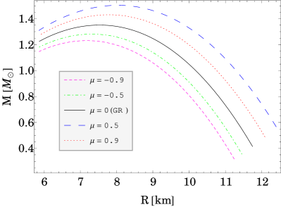
Figure 1: Mass-radius relation for isotropic sphere with $n=1$.

3 Isotropic Polytropes

Here, we study isotropic polytropes through two polytropic EoS [67] and develop LEE for both mass (baryonic) density $(\rho_{o})$ and energy density $(\rho)$ cases.

Case I

In this case, we take the polytropic EoS as

$$P=K\rho_{o}^{\gamma}=K\rho_{o}^{1+\frac{1}{n}}.$$ (17)

The correlation between mass (baryonic) density and energy density is expressed as

$$\rho=\rho_{o}+nP.$$

To develop the LEE, we define dimensionless variables as

$$\alpha=P_{c}/\rho_{c},\quad A^{2}=4\pi\rho_{c}/\alpha(n+1),\quad\psi_{o}^{n}=\rho_{o}/\rho_{oc},$$

$$r=\zeta/A,\quad\upsilon(\zeta)=m(r)A^{3}/(4\pi\rho_{c}),$$ (18)

where $c$ means that the corresponding term is evaluated at the center. Inserting these values in TOV equation, it follows that

$$\frac{a\zeta^{2}}{\alpha(n+1)}\left[\frac{L(n(1-n\alpha)+(n^{2}-1)\alpha\psi_{o})\psi_{o}^{-1}-\alpha(n+1)}{(1-n\alpha)+\left(n+1\right)\alpha\,\psi_{o}}\right]\frac{d\psi_{o}}{d\zeta}$$

$$-\zeta^{3}\psi_{o}^{n}\frac{\mu}{8\pi}((3-n)\alpha\psi_{o}-(1-n\alpha))-\upsilon-\alpha\zeta^{3}\psi_{o}^{n+1}=0,$$ (19)

where $L=\frac{\mu}{8\pi+2\mu}$ and $a=1-\frac{2(n+1)\alpha\upsilon}{\zeta}$. Substituting the dimensionless variables in Eq.(13), we obtain

$$\frac{d\upsilon}{d\zeta}=\zeta^{2}\psi_{o}^{n}((1-n\alpha+n\alpha\,\psi_{o})+\frac{1}{8\pi}\,{\mu\,\left(3(1-n\alpha)+\alpha\,\psi_{o}\left(3\,n-1\right)\right)}).$$ (20)

Now we combine Eqs.(19) and (20), it follows that

$$a\{L(n(1-n\alpha)+(n^{2}-1)\alpha\psi_{o})\psi_{o}^{-1}-\alpha(n+1)\}\frac{d^{2}\psi_{o}}{d\zeta^{2}}$$

$$+\frac{2}{\zeta}\frac{d\psi_{o}}{d\zeta}(a\{L(n(1-n\alpha)+(n^{2}-1)\alpha\psi_{o})\psi_{o}^{-1}-\alpha(n+1)\}$$

$$+\frac{1}{2}a(L(n^{2}-1)\alpha\psi_{o}^{-1}-L(n(1-n\alpha)+(n^{2}-1)\alpha\psi_{o})\psi_{o}^{-2})\zeta\frac{d\psi_{o}}{d\zeta}$$

$$-\zeta\alpha(n+1)(\zeta(\{L(n(1-n\alpha)+(n^{2}-1)\alpha\psi_{o})\psi_{o}^{-1}-\alpha(n+1)\})$$

$$\times(1-n\alpha+n\alpha\psi_{o}+\frac{1}{8\pi}\mu(3-3n\alpha+\alpha\psi_{o}(3n-1))\psi^{n}$$

$$-\frac{\upsilon}{\zeta^{2}}\{L(n(1-n\alpha)+(n^{2}-1)\alpha\psi_{o})\psi_{o}^{-1}-\alpha(n+1)\}+\frac{1}{2}\alpha\zeta(n+1)b\psi_{o}^{n}$$

$$+\frac{1}{2b}a\{L(n(1-n\alpha)+(n^{2}-1)\alpha\psi_{o})\psi_{o}^{-1}-\alpha(n+1)\}\frac{d\psi_{o}}{d\zeta}$$

$$+\frac{1}{16\pi}nb\mu\zeta(n((3-n)\alpha\psi_{o}+n\alpha-1)+(3-n)\alpha\psi_{o})\psi_{o}^{n-1})))$$

$$-(3\alpha\psi_{o}+1-n\alpha+n\alpha\psi_{o}+\frac{1}{8\pi}\mu(3-3n\alpha+\alpha\psi_{o}(3n-1))b\alpha(n+1)\psi_{o}^{n}$$

$$-\frac{3}{8\pi}b\mu\alpha(n+1)((3-n)\alpha\psi_{o}+n\alpha-1)\psi_{o}^{n}=0,$$ (21)

where $b=1-n\alpha+(n+1)\alpha\psi_{o}$. This is the LEE that describes the polytropic stars in the hydrostatic equilibrium. It is obvious that the above equation reduces to Eq.(34) in [38] when $\mu=0$.

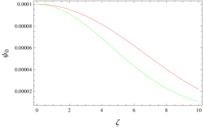
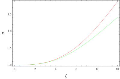
Figure 2: Plots of $\psi_{o}$ and $\upsilon$ corresponding to case I for $\mu=-0.9$, $n=0.5$ and $\alpha=0.1$ (red), $0.2$ (green).

Since Eqs.(19) and (20) are complicated, so, it is difficult to find exact solution of these equations. Thus, we find numerical solution of these equations by considering different values of the involved parameters. Figure 2 describes that the value of $\psi_{o}$ is maximum at the center and decreases as the radius increases. This provides a viable behavior of $\psi_{o}$ as it is positive inside the star and decreases as moves away from the center of the star. The graphical behavior of total mass is represented in Figure 2. This shows that the total mass has an increasing trend and is minimum at the center which represents compactness of the polytropic stars.

Case II

Here, we take the second polytropic EoS as

$$P=\emph{K}\rho^{\gamma}=\emph{K}\rho^{1+\frac{1}{n}},$$ (22)

where $\rho=\frac{\rho_{o}}{(1-\emph{K}\rho_{o}^{\frac{1}{n}})^{n}}$ and define another dimensionless variable as $\psi^{n}=\rho/\rho_{c}$ for this case. Kaisavelu et al. [68] generated superdense stellar structures obeying a polytropic EoS and also discussed their stability. The TOV equation and Eq.(13) turn out to be

$$a\zeta^{2}\frac{d\psi}{d\zeta}\left[\frac{L(n-\alpha(n+1)\psi)\psi^{-1}-\alpha(n+1)}{\alpha(n+1)(1+\alpha\psi)}\right]-\zeta^{3}\psi^{n}\frac{\mu}{8\pi}(3\alpha\psi-1)$$

$$-\upsilon-\alpha\zeta^{3}\psi^{n+1}=0,$$ (23)

$$\frac{d\upsilon}{d\zeta}=\zeta^{2}\psi^{n}(1+\frac{1}{8\pi}\mu(3-\alpha\psi)).$$ (24)

The corresponding LEE becomes

$$a(L(n-\alpha(n+1)\psi)\psi^{-1}-\alpha(n+1))\frac{d^{2}\psi}{d\zeta^{2}}+\frac{2}{\zeta}\frac{d\psi}{d\zeta}(a\{(L(n$$

$$-\alpha(n+1)\psi)\psi^{-1}-\alpha(n+1)\})-\frac{1}{2}a\zeta L\{(n-\alpha(n+1)\psi)\psi^{-2}$$

$$+\alpha(n+1)\psi^{-1}\}\frac{d\psi}{d\zeta}-\frac{1}{2c}a\zeta\alpha\{L(n-\alpha(n+1)\psi)\psi^{-1}+\alpha(n+1)\}\frac{d\psi}{d\zeta}$$

$$+\frac{1}{\zeta}\alpha(n+1)\upsilon\{L(n-\alpha(n+1)\psi)\psi^{-1}-\alpha(n+1)\}-\frac{1}{2}\alpha^{2}(n+1)^{2}c\zeta^{2}\psi^{n}$$

$$-\zeta^{2}\alpha(n+1)\{L(n-\alpha(n+1)\psi)\psi^{-1}-\alpha(n+1)\}\{1+\frac{1}{8\pi}\mu(3-\alpha\psi)\}\psi^{n}$$

$$-\frac{1}{16\pi}\zeta c\mu\alpha(n+1)(n(3\alpha\psi-1)+3\zeta\alpha\psi)\psi^{n-1})-3c(n+1)\alpha^{2}\psi^{n+1}$$

$$-c\alpha(n+1)\{1+\frac{1}{8\pi}\mu(3-\alpha\psi)\}\psi^{n}-\frac{3}{8\pi}c\mu\alpha(n+1)(3\alpha\psi-1)=0,$$ (25)

where $c=1+\alpha\psi$. This equation reduces to Eq.(42) in [38] when $\mu=0$. The numerical solution of Eqs.(23) and (24) is given in Figure 3. Figure 3 shows that the behavior of $\psi$ is physically viable as it is maximum at the center and decreases towards the surface boundary. It also represents that the total mass has increasing behavior and is minimum at the center. Equations (21) and (25) are two LEE that correspond to the mass (baryonic) density and total energy density, respectively. These are the nonlinear ordinary differential equations which describe the internal configuration of self-gravitating polytrophic stars and help to understand different astrophysical phenomena.

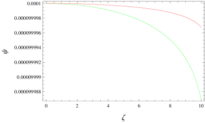
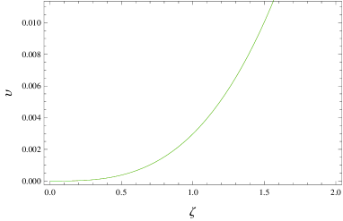
Figure 3: Plots of $\psi$ and $\upsilon$ versus $\zeta$ corresponding to case II for $\mu=-0.9$, $n=0.5$ and $\alpha=0.1$ (red), 0.2 (green).

3.1 Physical Features of Isotropic Polytropes

A physically acceptable stellar object must have monotonically decreasing density and pressure away from the center. It is shown in Figure 4 that the density as well as pressure of both isotropic models are positive and finite with a decreasing trend towards the boundary. Moreover, it is necessary that the energy-momentum tensor (representing normal matter distribution inside the compact structure) is consistent with the following energy conditions

$$\text{null energy condition:}\quad\rho+P\geq 0,\quad\rho+P\geq 0,$$

$$\text{weak energy condition:}\quad\rho\geq 0,\quad\rho+P\geq 0,$$

$$\text{strong energy condition:}\quad\rho+3P\geq 0,$$

$$\text{dominant energy condition:}\quad\rho-P\geq 0,$$

$$\text{trace energy condition:}\quad\rho-3P\geq 0$$

Figure 4 indicates that first three bounds are fulfilled for both isotropic models. The models are viable as the dominant and trace energy conditions are also satisfied as shown in Figure 5.

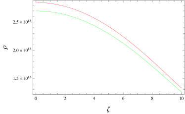
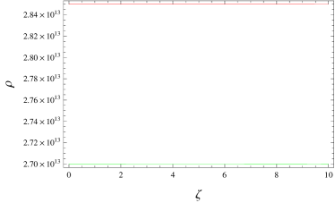
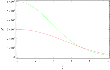
Figure 4: Plots of $\rho$ and $P$ versus $\zeta$ for $\mu=-0.9$, $n=0.5$ and $\alpha=0.1$ (red), 0.2 (green) for cases I (left) and II (right).

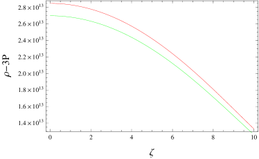
Figure 5: Plots of $\rho-P$ and $\rho-3P$ versus $\zeta$ for $\mu=-0.9$, $n=0.5$ and $\alpha=0.1$ (red), 0.2 (green) for cases I (left) and II (right).

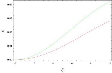
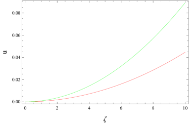
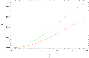
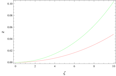
Figure 6: Plots of $u$ and $Z$ versus $\zeta$ for $\mu=-0.9$, $n=0.5$ and $\alpha=0.1$ (red), 0.2 (green) for cases I (left) and II (right).

The ratio of mass to radius provides a metric for the compactness of a self-gravitating system. This ratio, known as compactness factor $(u)$, must be less than $4/9$ throughout the interior of the sphere [69]. The compactness factor is further employed to calculate the possible redshift produced in an electromagnetic wave due to the cosmic object’s gravitational field. The redshift measured as

$$Z(r)=\frac{1-\sqrt{1-2u}}{\sqrt{1-2u}},$$

lies below 2 for isotropic structures [69]. Moreover, compactness of a structure increases if more matter is packed within the same radius. On the other hand, gravitational redshift measures the effect of the spherical object’s gravitational field on electromagnetic waves. Consequently, an increase in the compactness of the spherical stellar structure will lead to a stronger gravitational field, i.e., the redshift of electromagnetic waves will be higher. The compactness as well as redshift parameters related to both models (plotted in Figure 6) obey the required limits.

A fluid distribution is stable if a sound wave travels at a speed ($\nu^{2}=\frac{dP}{d\rho}$) less than that of light, i.e., the condition of causality does not fail at any point within the medium. Plots of sound speed in Figure 7 imply that the constructed models are stable. Further, the adiabatic index ($\Gamma=\frac{P+\rho}{P}\frac{dP}{d\rho}$) gauges the stiffness of the configuration. A stiff system (corresponds to $\Gamma>\frac{4}{3}$ [70]) is difficult to compress as a slight increase in density significantly enhances the outward pressure. The scenarios under consideration are stiff as they correspond to $\Gamma=3$ (refer to Figure 7).

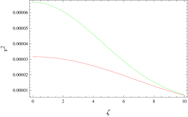
Figure 7: Plots of $\nu^{2}$ and $\Gamma$ versus $\zeta$ for $\mu=-0.9$, $n=0.5$ and $\alpha=0.1$ (red), 0.2 (green) for cases I (left) and II (right).

4 Anisotropic Polytropes

Anisotropy plays an important role in various dynamical phases of stellar evolution. Mostly stellar models are anisotropic in nature. The effect of anisotropy appears when the radial stress differs from the tangential stress. The anisotropic matter distribution is

$$\mathrm{T}_{\xi\eta}=(\rho+P_{\perp})u_{\xi}u_{\eta}-P_{\perp}g_{\xi\eta}+(P_{r}-P_{\perp})s_{\xi}s_{\eta},$$ (26)

where $s_{\xi}$ is the four-vector, $P_{r}$ and $P_{\perp}$ are radial and tangential pressures, respectively. The corresponding field equations and TOV equation are

$$\frac{1}{r^{2}}+e^{-\lambda}(\frac{\lambda^{\prime}}{r}-\frac{1}{r^{2}})=8\pi\rho+\mu(\rho-P_{r}-2P_{\perp}),$$ (27)

$$\frac{-1}{r^{2}}+e^{-\lambda}(\frac{\vartheta^{\prime}}{r}+\frac{1}{r^{2}})=8\pi P_{r}+\mu(\rho+3P_{r}+2P_{\perp}),$$ (28)

$$\frac{e^{-\lambda}}{4}(2\vartheta^{\prime\prime}+\vartheta^{\prime 2}-\lambda^{\prime}\vartheta^{\prime}+2\frac{(\vartheta^{\prime}-\lambda^{\prime})}{r})=8\pi P_{\perp}+\mu(\rho+P_{r}+4P_{\perp}),$$ (29)

$$P^{\prime}_{r}+\frac{\vartheta^{\prime}}{2}(\rho+P_{r})-\frac{2\Delta}{r}+\frac{\mu}{8\pi+2\mu}(\rho^{\prime}+P_{r}^{\prime}+2P_{\perp}^{\prime})=0,$$ (30)

where $\Delta=-\Pi=P_{\perp}-P_{r}$. Heintzmann and Hillebrandt [70] established a relation between radial and tangential pressures as

$$P_{\perp}=(1+q)P_{r},\quad q=\frac{3\epsilon}{2(\epsilon-1)},\quad\epsilon<1.$$ (31)

This relation is used to examine the effects of anisotropic stress on self-gravitating objects. Using this relation in the above equations, we have

$$\frac{1}{r^{2}}+e^{-\lambda}(\frac{\lambda^{\prime}}{r}-\frac{1}{r^{2}})=8\pi\rho+\mu(\rho-c_{1}P_{r}),$$ (35)

$$\frac{-1}{r^{2}}+e^{-\lambda}(\frac{\vartheta^{\prime}}{r}+\frac{1}{r^{2}})=8\pi P_{r}+\mu(\rho+c_{2}P_{r}),$$

$$\frac{e^{-\lambda}}{4}(2\vartheta^{\prime\prime}+\vartheta^{\prime 2}-\lambda^{\prime}\vartheta^{\prime}+2\frac{(\vartheta^{\prime}-\lambda^{\prime})}{r})=8\pi P_{\perp}+\mu(\rho+c_{3}P_{r}),$$

$$P^{\prime}_{r}+\frac{\vartheta^{\prime}}{2}(\rho+P_{r})-\frac{2\Delta}{r}+\frac{\mu}{8\pi+2\mu}(\rho^{\prime}+c_{1}P_{r}^{\prime})=0,$$

where $c_{1}=3+2q$, $c_{2}=5+2q$ and $c_{3}=5+4q$. Using Eqs.(12) and (35), we have

$$m^{\prime}=4\pi\rho r^{2}+\frac{\mu}{2}(\rho-c_{1}P_{r})r^{2}.$$ (36)

In the following, we use two polytropic EoS in terms of radial pressure defined in Eqs.(17) and (22) as

$$P_{r}=\emph{K}\rho_{o}^{\gamma}=\emph{K}\rho_{o}^{1+\frac{1}{n}},\quad P_{r}=\emph{K}\rho^{\gamma}=\emph{K}\rho^{1+\frac{1}{n}}.$$ (37)

We also plot the mass-radius curves for different values of $\mu$ by employing the relation $P_{r}=\emph{K}\rho^{2}$ along side Eqs.(36) and (37) (refer to Figure 8). We observe that mass of the stellar structure approaches to that of GR model as $\mu\rightarrow 0$.

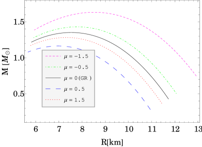
Figure 8: Mass-radius relation for anisotropic configuration with $n=2$.

Case I

We formulate LEE using the same procedure as in the isotropic case. The TOV equation in terms of dimensionless parameters becomes

$$a\zeta^{2}\frac{d\psi_{0}}{d\zeta}\bigg{[}P_{rc}(n+1)+\frac{P_{rc}}{\alpha}\psi_{0}^{-1}L(n(\alpha\psi_{0}(n+1)-(1-n\alpha))+(n+1)\alpha\psi_{0}c_{1})\bigg{]}$$

$$\times[P_{rc}(n+1)((n+1)\alpha\psi_{0}+(1-n\alpha))]^{-1}-\frac{2\Delta\psi_{0}^{-n}\zeta}{P_{rc}(n+1)}\frac{a}{b}+\upsilon+\alpha\zeta^{3}\psi_{0}^{n+1}$$

$$+\frac{\mu}{8\pi}\zeta^{3}\psi_{0}^{n}((1-n\alpha)+(n+c_{2})\alpha\psi_{0})=0,$$ (38)

where $\alpha=P_{rc}/\rho_{c}$. The conservation of mass in terms of dimensionless variables takes the form

$$\frac{d\upsilon}{d\zeta}=\zeta^{2}\psi_{o}^{n}\left(((1-n\alpha)+n\alpha\psi_{o})+\frac{\mu}{8\pi}((1-n\alpha)+(n-c_{1})\alpha\psi_{o})\right).$$ (39)

Manipulating Eqs.(38) and (39), it follows that

$$a\left[1+\frac{L(n(1-n\alpha+(n+1)\alpha\psi_{o})+\alpha\psi_{o}c_{1}(n+1))}{\psi_{o}\alpha(n+1)}\right]\frac{d^{2}\psi_{o}}{d\zeta^{2}}+\frac{1}{P_{rc}(n+1)\zeta}$$

$$\times\frac{d\psi_{o}}{d\zeta}\bigg{[}a\left(P_{rc}(n+1)+\frac{P_{rc}L(n(1-n\alpha+(n+1)\alpha\psi_{o})+\alpha\psi_{o}c_{1}(n+1))}{\psi_{o}\alpha}\right)$$

$$+aP_{rc}(n+1)+2\bigg{[}P_{rc}(n+1)+P_{rc}L(n(1-n\alpha+(n+1)\alpha\psi_{o})$$

$$+\alpha\psi_{o}c_{1}(n+1))(\psi_{o}\alpha)^{-1}\bigg{]}\alpha\upsilon(n+1)\zeta^{-1}+\frac{aP_{rc}}{\alpha\psi_{o}}L\bigg{[}n(1-n\alpha$$

$$+(n+1)\alpha\psi_{o})+\alpha\psi_{o}c_{1}(n+1)\bigg{]}-a\zeta P_{rc}L\bigg{[}n(1-n\alpha$$

$$+(n+1)\alpha\psi_{o})+\alpha\psi_{o}c_{1}(n+1)\bigg{]}(\alpha\psi_{o}^{2})^{-1}\frac{d\psi_{o}}{d\zeta}-2\zeta^{2}(n+1)\alpha\bigg{[}1-n\alpha$$

$$+n\alpha\psi_{o}+\frac{1}{8\pi}\mu(1-n\alpha+n\alpha\psi_{o}-c_{1}\alpha\psi_{o})\bigg{]}\bigg{(}P_{rc}(n+1)$$

$$+\frac{P_{rc}L(n(1-n\alpha+(n+1)\alpha\psi_{o})+\alpha\psi_{o}c_{1}(n+1))}{\psi_{o}\alpha}\bigg{)}\psi_{o}^{-n}-a\alpha\zeta(n+1)\frac{1}{b}$$

$$\times\left(P_{rc}(n+1)+\frac{P_{rc}L(n(1-n\alpha+(n+1)\alpha\psi_{o})+\alpha\psi_{o}c_{1}(n+1))}{\psi_{o}\alpha}\right)\frac{d\psi_{o}}{d\zeta}$$

$$+b\zeta\alpha(n+1)^{2}\alpha P_{rc}\psi_{o}^{n}+\frac{LP_{rc}(n+1)(n+c_{1})}{\psi_{o}}\frac{d\psi_{o}}{d\zeta}\bigg{]}-\frac{2\psi_{o}^{-n}}{\alpha P_{rc}\zeta(n+1)}$$

$$\times\left(a\frac{d\Delta}{d\zeta}-\frac{na\Delta}{\psi_{o}}\frac{d\psi_{o}}{d\zeta}+\frac{2\alpha\upsilon(n+1)\Delta}{\zeta^{2}}+\frac{a\Delta}{\zeta}-\frac{a\alpha(n+1)\Delta}{b}\frac{d\psi_{o}}{d\zeta}\right.$$

$$\left.-2\zeta\alpha\psi_{o}^{n}\Delta\left[1-n\alpha+n\alpha\psi_{o}+\frac{1}{8\pi}\mu(1-n\alpha+n\alpha\psi_{o}-c_{1}\alpha\psi_{o})\right](n+1)\right)$$

$$+b\psi_{o}^{n}\left(3\alpha\psi_{o}+\left[1-n\alpha+n\alpha\psi_{o}+\frac{1}{8\pi}\mu(1-n\alpha+n\alpha\psi_{o}-c_{1}\alpha\psi_{o})\right]\right)$$

$$+\frac{1}{8\pi}\frac{d\psi_{o}}{d\zeta}b\mu\zeta\psi_{o}^{n-1}\bigg{(}n(1-n\alpha+(n+c_{2})\alpha\psi_{o})+\alpha\psi_{o}(n+c_{2})\bigg{)}$$

$$+\frac{3}{8\pi}b\mu\bigg{(}1-n\alpha+(n+c_{2})\alpha\psi_{o}\bigg{)}\psi_{o}^{n}=0.$$ (40)

This is the LEE equation which helps to comprehend the internal structure of the anisotropic polytropic stars. It is interesting to mention here that the above equation reduces to GR equation (58) in [38] when the model parameter ($\mu$) vanishes.

Case II

In this case, the TOV equation reduces to

$$a\zeta^{2}\frac{d\psi}{d\zeta}\left[\frac{P_{rc}(n+1)+\frac{P_{rc}}{\alpha}\psi^{-1}L(n+(n+1)\alpha\psi c_{1})}{P_{rc}(n+1)(1+\alpha\psi)}\right]+\alpha\zeta^{3}\psi^{n+1}$$

$$-\frac{2a\Delta\psi^{-n}\zeta}{P_{rc}(n+1)(1+\alpha\psi)}+\upsilon+\frac{\mu}{8\pi}(1+\alpha c_{2}\psi)\zeta^{3}\psi^{n}=0.$$ (41)

Using dimensionless variables in Eq.(36), we have

$$\frac{d\upsilon}{d\zeta}=\zeta^{2}\psi^{n}\left[1+\frac{\mu}{8\pi}(1-\alpha c_{1}\psi)\right].$$ (42)

The resulting LEE turns out to be

$$a\left[1+\frac{L(n+\alpha\psi c_{1}(n+1))}{\psi\alpha(n+1)}\right]\frac{d^{2}\psi}{d\zeta^{2}}-\frac{2\psi^{-n}}{\zeta P_{rc}(n+1)}\left[a\frac{d\Delta}{d\zeta}-\frac{na\Delta}{\psi}\frac{d\psi}{d\zeta}+\frac{a\Delta}{\zeta}\right.$$

$$\left.+\frac{2(n+1)\alpha\upsilon\Delta}{\zeta^{2}}-\frac{a\alpha\Delta}{c}\frac{d\psi}{d\zeta}-2\Delta\zeta\alpha(n+1)\left(1+\frac{1}{8\pi}{\mu(1-c_{1}\alpha\psi)}\right)\psi^{n}\right]$$

$$+\frac{1}{\zeta P_{rc}(n+1)}\frac{d\psi}{d\zeta}\bigg{[}a(P_{rc}(n+1)+\frac{P_{rc}L(n+\alpha\psi c_{1}(n+1))}{\alpha\psi})$$

$$+\frac{2}{\zeta}(n+1)\alpha\upsilon\left(P_{rc}(n+1)+\frac{P_{rc}L(n+\alpha\psi c_{1}(n+1))}{\alpha\psi}\right)+\alpha P_{rc}(n+1)$$

$$+\frac{aP_{rc}L(n+\alpha\psi c_{1}(n+1))}{\alpha\psi}+\frac{\zeta\alpha P_{rc}Lc_{1}(n+1)}{\psi}\frac{d\psi}{d\zeta}-\frac{\zeta a\alpha}{c}\bigg{[}P_{rc}(n+1)$$

$$+\frac{P_{rc}L(n+\alpha\psi c_{1}(n+1))}{\alpha\psi}\bigg{]}\frac{d\psi}{d\zeta}-2\alpha\zeta^{2}\psi^{n}(n+1)\bigg{[}P_{rc}(n+1)$$

$$+\frac{P_{rc}L(n+\alpha\psi c_{1}(n+1))}{\alpha\psi}\bigg{]}\left(1+\frac{1}{8}\frac{\mu(1-c_{1}\alpha\psi)}{\pi}\right)+\frac{aP_{rc}}{\alpha\psi^{2}}\frac{d\psi}{d\zeta}$$

$$-c\zeta\alpha P_{rc}(n+1)^{2}\psi^{n}\bigg{]}+c\psi^{n}\left(3\alpha\psi+1+\frac{1}{8}\frac{\mu(1-c_{1}\alpha\psi)}{\pi}\right)$$

$$+\frac{1}{8\pi}c\mu\zeta\psi^{n-1}(n+(n+1)\alpha\psi c_{2})\frac{d\psi}{d\zeta}+\frac{3}{8\pi}\mu c\psi^{n}(1+\alpha c_{2}\psi)=0.$$ (43)

In the limiting case ($\mu=0$), we can recover Eq.(60) of GR in [38].

In order to proceed further with the modeling of a compact object, we need some additional information based on the particular physical problem under consideration. For this purpose, we define specific anisotropy $(\Delta)$ for the modeling of relativistic anisotropic stars [71, 72] which helps to study the effect of anisotropy of the structure of the compact object.

5 Modeling of Anisotropic Polytropes

In this section, we use the method used in [71] to obtain specific models. This will help to find solutions for anisotropic matter. This procedure is briefly mentioned as follows. We assume anisotropic factor as

$$\bigtriangleup=Cf(P_{r},r)(\rho+P_{r})r^{N},$$ (44)

where $C$ is the anisotropic parameter. It is mentioned here that the function $f$ and the number $N$ are specified for each model. We further assume that

$$f(P_{r},r)r^{N-1}=\frac{\vartheta^{\prime}}{2}.$$ (45)

Using Eqs.(44) and (45) in (36), we have

$$P_{r}^{\prime}=-\frac{\vartheta^{\prime}}{2}h(\rho+P_{r})-L(\rho^{\prime}+P_{r}^{\prime}c_{1}),$$ (46)

where $h=1-2C$. For the sake of convenience, we assume that $h$ is constant which doest not mean that either pressure is constant. Thus we obtain the following two equations for the case I as

$$a\zeta^{2}\frac{d\psi_{0}}{d\zeta}\left[\frac{\alpha(n+1)+L(n(\alpha\psi_{o}(n+1)+(1-n\alpha))+\alpha(n+1)c_{1}\psi_{o})\psi_{o}^{-1}}{\alpha(n+1)((1-n\alpha)+(n+1)\alpha\psi_{o})}\right]$$

$$+h\left[\upsilon+\zeta^{3}\alpha\psi_{o}^{n+1}+\frac{\mu}{8\pi}(\alpha\psi_{o}(n+c_{2})+(1-n\alpha))\zeta^{3}\psi_{o}^{n}\right]=0,$$ (47)

$$\frac{d\upsilon}{d\zeta}=\zeta^{2}\psi_{o}^{n}\left(((1-n\alpha)+n\alpha\psi_{o})+\frac{\mu}{8\pi}((1-n\alpha)+(n-c_{1})\alpha\psi_{o})\right).$$ (48)

The analytic solution of these equations is too difficult to find due to their complicated nature. Therefore, we solve these equations numerically by taking different values of the involved parameters.

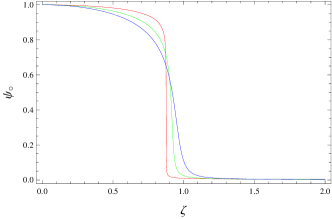
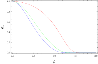
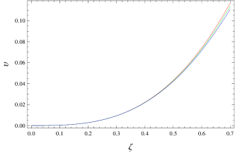
Figure 9: Plots of $\psi_{o}$ and $\upsilon$ corresponding to anisotropic case I for $\mu=1.5$, $c_{1}=2$, $h=0.5$ (red), 1 (green), 1.5 (blue) with $\alpha=0.1$ (left), $n=1$ (left) and $\alpha=1$ (right), $n=0.5$ (right).

Figure 9 shows that the value of $\psi_{o}$ at the center is maximum and decreases as the radius increases. Thus there is a decreasing behavior of the curve for the involved parameters. Also, we obtain large values of $\psi_{o}$ corresponding to a small value of $h$. Hence, there is a viable behavior of $\psi_{o}$, i.e., it must be non-negative inside the star and decreases as we move away from the center of the star. The graph of total mass for different values of $h$ is represented in Figure 9. We have a larger value of $\upsilon$ for a smaller value of $h$ and there is no irregular pattern in both plots. This shows that at the center, the value of $\upsilon$ is minimum and gradually increases as we move away from the center. Thus, for small values of the anisotropic parameter, we have a more compact model. Similarly, for case II, we have

$$a\zeta^{2}\frac{d\psi}{d\zeta}\left[\frac{\alpha(n+1)+L(n+\psi c_{1}\alpha(n+1))\psi^{-1}}{\alpha(n+1)(1+\alpha\psi)}\right]$$

$$+h\left[\upsilon+\zeta^{3}\alpha\psi^{n+1}+\frac{\mu}{8\pi}(1+\alpha c_{2}\psi)\zeta^{3}\psi^{n}\right]=0,$$ (49)

$$\frac{d\upsilon}{d\zeta}=\zeta^{2}\psi^{n}\left[1+\frac{\mu}{8\pi}(1-\alpha c_{1}\psi)\right].$$ (50)

The numerical solution of these equations is represented in Figure 10. Figure 10 shows that the value of $\psi$ is maximum at the center and decreases towards the surface boundary. Figure 10 indicates that we have a more compact model for small values of anisotropic parameter.

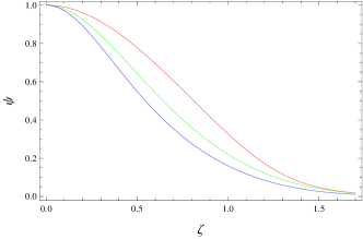
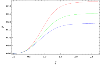
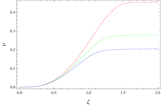
Figure 10: Plots of $\psi$ and $\upsilon$ corresponding to anisotropic case II for $\mu=1.5$, $c_{1}=2$ and $h=0.5$ (red), 1 (green), 1.5 (blue) with $\alpha=1$ (left), $n=1$ (left) and $\alpha=0.1$ (right) and $n=2$ (right).

5.1 Physical Features of Anisotropic Polytropes

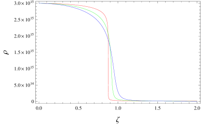
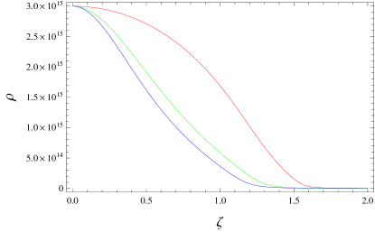
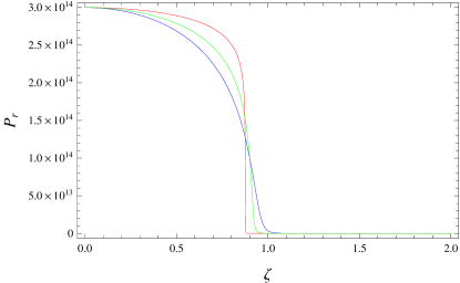
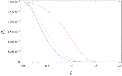
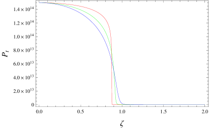
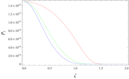
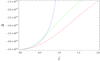
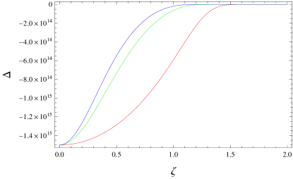
Figure 11: Plots of $\rho,~{}P_{r},~{}P_{\perp}$ and $\Delta$ corresponding to anisotropic case I for $\mu=1.5$, $c_{1}=2$, $h=0.5$ (red), 1 (green), 1.5 (blue) with $\alpha=0.1$ (left), $n=1$ (left) and $\alpha=1$ (right), $n=0.5$ (right).

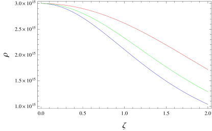
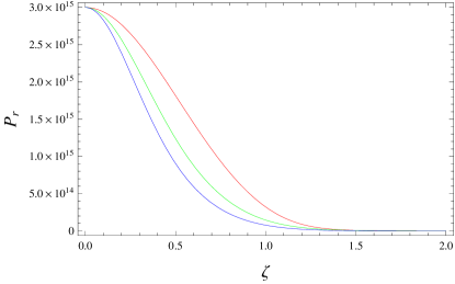
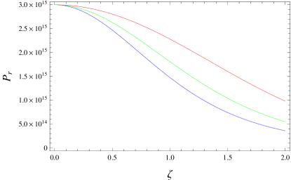
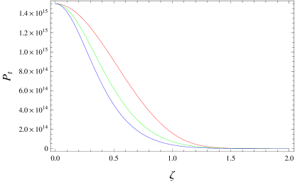
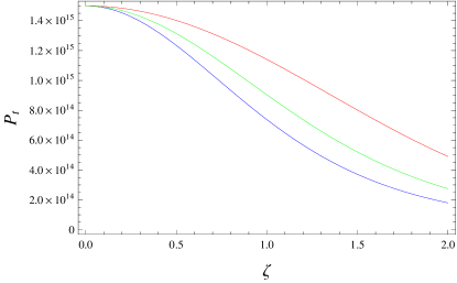
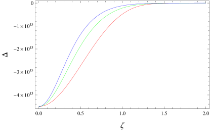
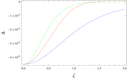
Figure 12: Plots of $\rho$, $P_{r}$, $P_{\perp}$ and $\Delta$ corresponding to anisotropic case II for $\mu=1.5$, $c_{1}=2$ and $h=0.5$ (red), 1 (green), 1.5 (blue) with $\alpha=1$ (left), $n=1$ (left) and $\alpha=0.1$ (right), $n=2$ (right).

In this subsection, we explore different attributes of the anisotropic setups for different values of the parameters. The matter variables of anisotropic polytropes monotonically decrease away from the center in both scenarios as depicted in Figures 11 and 12. An increase in the state parameters is noted as $h$ increases. However, in case I, the density as well as radial/tangential pressure initially increase and then decrease corresponding to higher values of $h$ when $\alpha=0.1$ and $n=1$. Moreover, the anisotropy is negative which indicates the presence of an attractive force within the spherical structures. The energy bounds related to anisotropic systems are

$$\text{null energy condition:}\quad\rho+P_{r}\geq 0,\quad\rho+P_{\perp}\geq 0,$$

$$\text{weak energy condition:}\quad\rho\geq 0,\quad\rho+P_{r}\geq 0,\quad\rho+P_{\perp}\geq 0,$$

$$\text{strong energy condition:}\quad\rho+P_{r}+2P_{\perp}\geq 0,$$

$$\text{dominant energy condition:}\quad\rho-P_{r}\geq 0,\quad\rho-P_{\perp}\geq 0,$$

$$\text{trace energy condition}\quad\rho-P_{r}-2P_{t}\geq 0.$$

As anisotropic models I and II have positive energy density and pressures, therefore the null, weak and strong energy conditions are satisfied. Figures 13 and 14 show that the anisotropic models are viable for the considered values of the parameters.

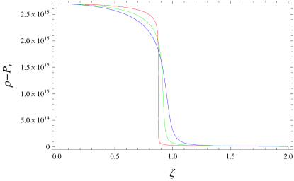
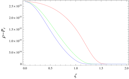
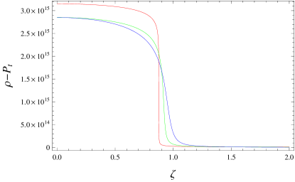
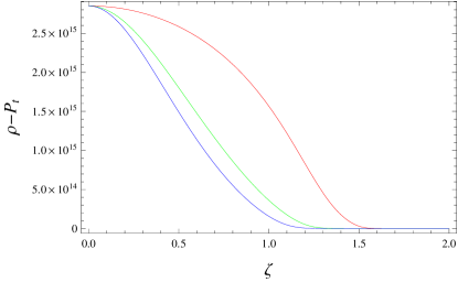
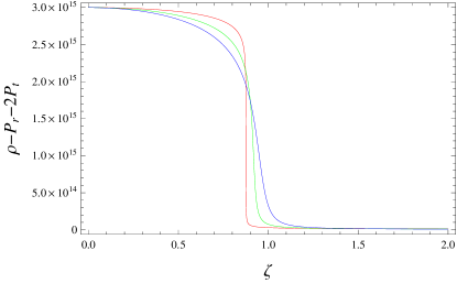
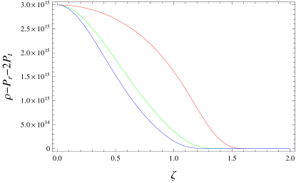
Figure 13: Plots of $\rho-P_{r}$, $\rho-P_{t}$ and $\rho-P_{r}-2P_{t}$ corresponding to anisotropic case I for $\mu=1.5$, $c_{1}=2$, $h=0.5$ (red), 1 (green), 1.5 (blue) with $\alpha=0.1$ (left), $n=1$ (left) and $\alpha=1$ (right), $n=0.5$ (right).

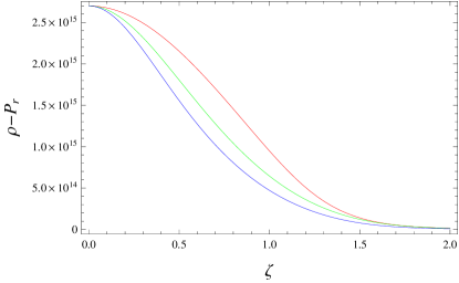
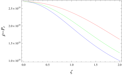
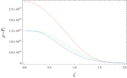
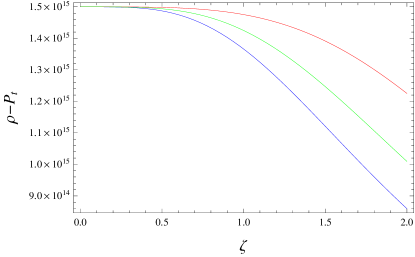
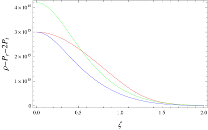
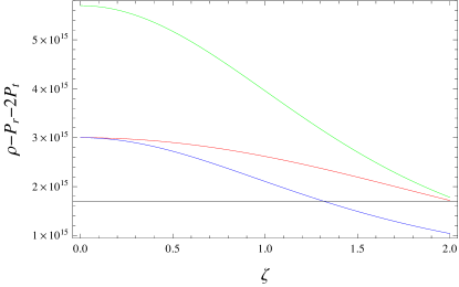
Figure 14: Plots of $\rho-P_{r}$, $\rho-P_{t}$ and $\rho-P_{r}-2P_{t}$ corresponding to anisotropic case II for $\mu=1.5$, $c_{1}=2$ and $h=0.5$ (red), 1 (green), 1.5 (blue) with $\alpha=1$ (left), $n=1$ (left) and $\alpha=0.1$ (right), $n=2$ (right).

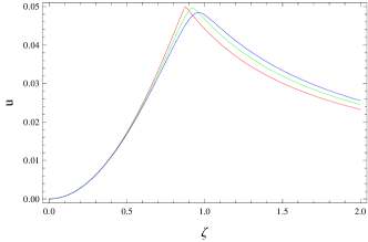
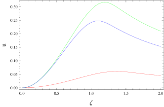
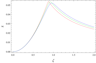
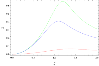
Figure 15: Plots of $u$ and $Z$ corresponding to anisotropic case I for $\mu=1.5$, $c_{1}=2$, $h=0.5$ (red), 1 (green), 1.5 (blue) with $\alpha=0.1$ (left), $n=1$(left) and $\alpha=1$ (right), $n=0.5$ (right).

The upper limit of compactness factor remains unchanged for anisotropic configurations whereas the upper bound of redshift increases to 5.211 [73]. It is observed from Figures 15 and 16 that these parameters comply with their required limits for cases I and II. We employ causality condition ($\nu_{r}^{2}=\frac{dP_{r}}{d\rho}<1$ and $\nu_{t}^{2}=\frac{dP_{t}}{d\rho}<1$ where $\nu_{r}^{2}$ and $\nu_{t}^{2}$ radial and tangential speeds of sound, respectively) to determine the stability of the anisotropic configurations. Figure 17 displays that the first anisotropic model is consistent with causality criterion whereas the second model is unstable for $\alpha=n=1$ (refer to Figure 18). Moreover, the model constructed in case I is stiff as the radial adiabatic index $\Gamma_{r}=\frac{P_{r}+\rho}{P_{r}}\frac{dP_{r}}{d\rho}$ is greater than $4/3$ throughout the internal configuration. On the other hand, $\Gamma_{r}<\frac{4}{3}$ in the second scenario for $\alpha=0.1$ and $n=2$. In relativistic scenario, Moustakidis [74] imposed an additional condition on adiabatic index. He proposed that $\Gamma_{r}$ must be greater than the critical value $\Gamma_{r\text{(critical)}}=\frac{4}{3}+\frac{19}{21}u$. Recently, the critical value of adiabatic index was also used to investigate the behavior of decoupled solutions [75]. We have plotted the critical values of adiabatic index in Figures 17 and 18. It is noted that $\Gamma_{r}$ is greater than the critical value for both case I and II.

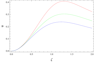
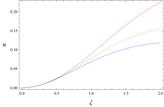
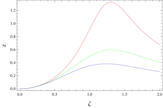
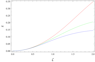
Figure 16: Plots of $u$ and $Z$ corresponding to anisotropic case II for $\mu=1.5$, $c_{1}=2$ and $h=0.5$ (red), 1 (green), 1.5 (blue) with $\alpha=1$ (left), $n=1$ (left) and $\alpha=0.1$ (right), $n=2$ (right).

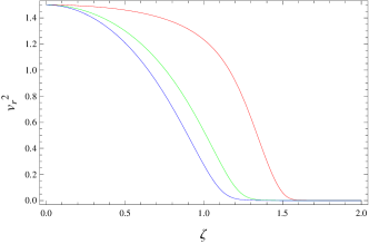
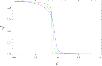
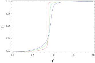
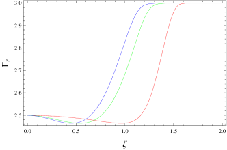
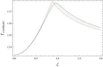
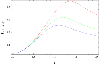
Figure 17: Plots of $\nu_{r}^{2}$, $\nu_{t}^{2}$, $\Gamma_{r}$ and $\Gamma_{r\text{(critical)}}$ corresponding to anisotropic case I for $\mu=1.5$, $c_{1}=2$, $h=0.5$ (red), 1 (green), 1.5 (blue) with $\alpha=0.1$ (left), $n=1$ (left) and $\alpha=1$ (right), $n=0.5$ (right).

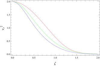
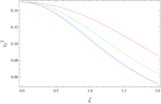
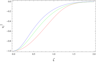
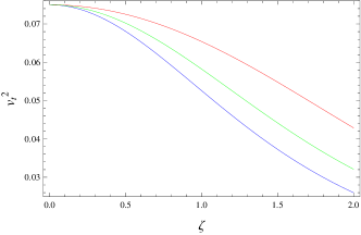
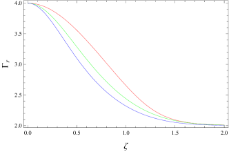
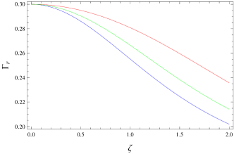
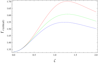
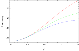
Figure 18: Plots of $v_{r}^{2}$, $v_{t}^{2}$, $\Gamma_{r}$ and $\Gamma_{r\text{(critical)}}$ corresponding to anisotropic case II for $\mu=1.5$, $c_{1}=2$ and $h=0.5$ (red), 1 (green), 1.5 (blue) with $\alpha=1$ (left), $n=1$(left) and $\alpha=0.1$ (right), $n=2$ (right).

Now, we compute the Tolman mass, which measures the gravitational mass, defined as [76]

$$m_{\mathrm{T}}=\frac{1}{2}r^{2}e^{\frac{{\vartheta-\lambda}}{2}}\vartheta^{\prime}.$$ (51)

Substituting Eq.(35) with mass function in Eq.(51), we have

$$m_{\mathrm{T}}=e^{\frac{{\vartheta+\lambda}}{2}}\bigg{[}m+r^{3}(4\pi P_{r}+\frac{\mu}{2}(\rho+c_{2}P_{r}))\bigg{]}.$$ (52)

For the case I, we use Eq.(18) in Eq.(35) and obtain

$$P_{r}=K\rho_{rc}^{1+\frac{1}{n}}\psi_{0}^{n+1},\quad\rho=\rho_{0c}\psi_{0}^{n}(1+nk\rho_{0c}^{1/n}\psi_{0}).$$ (53)

The resulting TOV equation yields

$$2(n+1)\beta d\psi_{0}+hd\vartheta[1+\beta\psi_{0}(n+1)]+L(n(1+n\beta\psi_{0})$$

$$+\beta\psi_{0}(n+c_{1}(1+n)))d\psi_{0}=0,$$ (54)

where $\beta=\frac{\alpha}{1-n\alpha}$. Integrating this equation, it follows that

$$e^{\vartheta}=\frac{H}{[\psi_{0}^{nL}(1+(n+1)\beta\psi_{0})^{1+c_{1}L}]^{\frac{2}{h}}},$$ (55)

where $H$ is an integration constant. Initial condition at the center ($r=0,~{}\psi_{0}=1$) yields $H$ and hence

$$e^{\vartheta}=e^{\vartheta_{c}}\frac{[(1+(n+1)\beta)^{1+c_{1}L}]^{\frac{2}{h}}}{[\psi_{0}^{nL}(1+(n+1)\beta\psi_{0})^{1+c_{1}L}]^{\frac{2}{h}}}.$$ (56)

Using the matching conditions defined in Eq.(16), we obtain

$$e^{\vartheta}=\left(1-\frac{2M}{r_{\Sigma}}\right)\frac{[(I^{nL}((1-n\alpha)+(n+1)\alpha I)^{1+c_{1}L}]^{\frac{2}{h}}}{[\psi_{0}^{nL}((1-n\alpha)+(n+1)\alpha\psi_{0})^{1+c_{1}L}]^{\frac{2}{h}}}.$$ (57)

Substituting this value in Eq.(52), we have

$$\upsilon_{\mathrm{T}}=(\upsilon+\zeta^{3}\psi_{0}^{n}(\alpha\psi_{0}+\frac{\mu}{8\pi}((1-n\alpha)+(n+c_{2})\alpha\psi_{0})))$$

$$\times\frac{(a_{\sum})^{1/2}}{(a)^{1/2}}\frac{[(I^{nL}((1-n\alpha)+(n+1)\alpha I)^{1+c_{1}L}]^{\frac{1}{h}}}{[\psi_{0}^{nL}((1-n\alpha)+(n+1)\alpha\psi_{0})^{1+c_{1}L}]^{\frac{1}{h}}},$$ (58)

where $\upsilon_{\mathrm{T}}=\frac{m_{\mathrm{T}}A^{3}}{4\pi\rho_{c}}$.

Similarly, for the case II, the TOV equation reduces to

$$2\alpha\psi(1+n)d\psi+h\psi(1+\alpha\psi)d\vartheta+L(n+\alpha c_{1}(1+n)\psi)d\psi=0.$$ (59)

Proceeding in the same way as for the case I, we have

$$e^{\vartheta}=\left(1-\frac{2M}{r_{\Sigma}}\right)\frac{[J^{nL}(1+\alpha J)^{(1+c_{1}L)(1+n)-nL}]^{\frac{2}{h}}}{[\psi^{nL}(1+\alpha\psi)^{(1+c_{1}L)(1+n)-nL}]^{\frac{2}{h}}}.$$ (60)

Substituting this value in Eq.(52), it follows that

$$\upsilon_{\mathrm{T}}=(\upsilon+\zeta^{3}\psi^{n}(\alpha\psi+\frac{\mu}{8\pi}((1+c_{2}\alpha\psi))))\frac{(a_{\Sigma})^{1/2}}{(a)^{1/2}}$$

$$\times\frac{[J^{nL}(1+\alpha J)^{(1+c_{1}L)(1+n)-nL}]^{\frac{1}{h}}}{[\psi^{nL}((1+\alpha\psi)^{(1+c_{1}L)(1+n)-nL}]^{\frac{1}{h}}},$$ (61)

where $I=\frac{\mu(n\alpha-1)}{\alpha(8\pi+(n+c_{2}))}$ and $J=\frac{-\mu}{8\pi+\mu c_{2}}$.

In order to explore the distribution of Tolman mass through the sphere during the slow and adiabatic process, the following dimensionless variables are introduced

$$x=\frac{r}{r_{\Sigma}}=\frac{\zeta}{\tilde{A}},\indent y=\frac{M}{r_{\Sigma}},\indent\tilde{m}=\frac{m}{M},\indent\tilde{A}=r_{\Sigma}A.$$ (62)

The Tolman mass for both cases (I and II) in terms of above variables takes the form

$$\upsilon_{\mathrm{T}} = (\upsilon+x^{3}\tilde{A}^{3}\psi_{0}^{n}(\alpha\psi_{0}+\frac{\mu}{8\pi}((1-n\alpha)+(n+c_{2})\alpha\psi_{0})))$$ (63)

$$\times \frac{\left[(I^{nL}((1-n\alpha)+(n+1)\alpha I)^{1+c_{1}L}\right]^{\frac{1}{h}}}{\left[\psi_{0}^{nL}((1-n\alpha)+(n+1)\alpha\psi_{0})^{1+c_{1}L}\right]^{\frac{1}{h}}}$$

$$\times \left(\frac{x(1-2y)}{x-2\alpha(n+1)\upsilon/\tilde{A}}\right)^{1/2},$$

$$\upsilon_{\mathrm{T}} = (\upsilon+x^{3}\tilde{A}^{3}\psi^{n}(\alpha\psi+\frac{\mu}{8\pi}((1+c_{2}\alpha\psi))))$$ (64)

$$\times \left[\frac{x(1-2y)}{x-2\alpha(n+1)\upsilon/\tilde{A}}\right]^{1/2}\frac{\left[J^{nL}(1+\alpha J)^{(1+c_{1}L)(1+n)-nL}\right]^{\frac{1}{h}}}{\left[\psi^{nL}(1+\alpha\psi)^{(1+c_{1}L)(1+n)-nL}\right]^{\frac{1}{h}}},$$

respectively. We note that $\tilde{A}=\zeta_{\Sigma}$ and Eqs.(18) and (62), we obtain

$$y=\alpha(n+1)\frac{\upsilon_{\Sigma}}{\zeta_{\Sigma}}.$$ (65)

This shows that $y$ depends on the anisotropy parameter $h$. This means that $y$ is constant for a pair $(n,\alpha)$ when $\upsilon_{\Sigma}/\zeta_{\Sigma}=constant$ which is possible only for every value of $h$. It is noted that the potential at the surface is uniquely related to each anisotropic and relativistic polytropes.

The behavior of the surface parameter $y$ corresponding to anisotropic parameter plays an important role in analyzing the compactness of the polytropic stars. For case I, the plot between $y$ and anisotropy parameter is shown in Figure 19. This describes that the value of $y$ decreases as the anisotropy parameter increases, which means that the degree of compactness of the model decreases as anisotropy increases and vice-versa. Similar behavior is obtained for the case II shown in Figure 20.

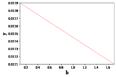
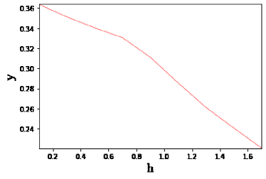
Figure 19: Plots of $y$ versus $h$ for $\mu=1.5$, $c_{1}=2$, $\alpha=0.1$ (left), $n=2$ (left), $\alpha=1$ (right) and $n=1$ (right).

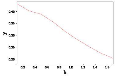
Figure 20: Plots of $y$ versus $h$ for $\mu=1.5$ and $c_{1}=2$, $n=1$, $\alpha=0.1$ (left) and $\alpha=1$ (right).

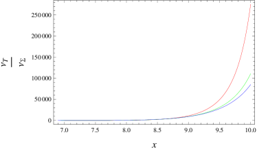
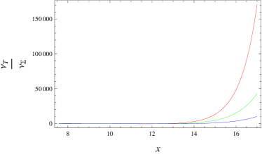
Figure 21: Plots of $\frac{\upsilon_{\mathrm{T}}}{\upsilon_{\Sigma}}$ versus $x$ for $\mu=1.5$, $c_{1}=2$, $c_{2}=4$ and $h=0.5$ (red), 1(green), 1.5(blue), $\alpha=0.1$ (left), $n=2$ (left), $\alpha=1$ (right) and $n=1$ (right).

The correspondence between $y$ and $h$ leads to stability of the models except where the cases for such a correspondence cannot be obtained. For this purpose, we explore the behavior of Tolman mass (normalized by the total mass) within the sphere to see the interesting features of the proposed model. Figure 21 (left) implies that when we switch from less compact (large anisotropy) to the large compact configuration (less anisotropy), the Tolman mass tends to concentrate at the outer region of the sphere. The Tolman mass has smaller values in the inner region of a star as we move from the large anisotropy to the small in the contraction process. Similar behavior of the Tolman mass is found in the case II shown in Figure 21 (right). In this case, as we move from a small compact to a large compact configuration, the Tolman mass appears to be condensed at the outer region of the sphere.

6 Conclusions

In this paper, we have studied the isotropic/anisotropic polytropes for a specific model of $f(\mathcal{R},\mathrm{T})$ theory. We have considered two polytropic EoS with hydrostatic equilibrium conditions to construct the LEE. We have used Darmois formalism for the smooth matching of interior and exterior spacetimes. We have taken mass (baryonic) density as well as energy density to formulate the TOV and mass equations in terms of dimensionless variables. The coupling of these two equations represents a polytrope in hydrostatic equilibrium. We have also examined different physical aspects (mass-radius relation, behavior of matter variables, compactness, redshift, viability and stability) of compact structures corresponding to isotropic/ anisotropic polytropic EoS for different values of the parameters. It has been noted that increase in $\alpha$ decreases the density of the isotropic solutions whereas more pressure is generated for higher values of $\alpha$. Moreover, these solutions are viable as well as stable for $f(\mathcal{R},\mathrm{T})=\mathcal{R}+2\mu\mathrm{T}$ when $\chi<0$. The compactness, redshift and adiabatic index also comply with the desired limits.

We have then discussed anisotropic polytropes for two cases. We have developed the LEE which is then integrated through analytical approach. The distributions that represent the polytropes, also determine the compact objects such as neutron stars and Super-Chandrasekhar white dwarfs. The anisotropic pressure and relativistic effects cannot be neglected in such configurations. We have transformed the system into a dimensionless form that reduces the computational work. The decreasing behavior of the surface potential for the anisotropic parameter shows compact polytropes. The graphical analysis of both anisotropic cases reveals that the related state determinants are positive with a decreasing behavior towards the surface for $\mu=1.5$. Negative anisotropy implies that pressure in the radial direction is greater than that in the transverse direction. Further, the anisotropic polytropes are composed of normal matter as they are consistent with the energy bounds. Finally, the first anisotropic solution is stable with respect to causality criterion whereas the second solution obeys causality condition for $\alpha=0.1$ and $n=2$. However, the adiabatic index of the second model is less than $\frac{4}{3}$ for $\alpha=0.1$ and $n=2$. Thus, the resulting solutions can be used to construct compact spherical models.

Finally, we have explored the Tolman mass which helps to understand stability of the models. The efficiency with which the Tolman mass is reduced in the inner region and concentrated in the outer region is determined by the anisotropic parameter. The sharp reduction of the Tolman mass in the interior region of the sphere for smaller values of anisotropy parameter indicates more compact and more stable configuration as compared to large values of the anisotropy. We have found that both isotropic/anisotropic polytropes are more viable and stable as compared to GR. It is worthwhile to mention here that all our results reduce to GR [38] when the model parameter vanishes.

References

- [1] Eicher, D.J. The New Cosmos Answering Astronomy Big Questions (Cambridge University Press, 2015).
- [2] Hinshaw, G. et al.: Astrophys. J. Suppl. 148(2003)135.
- [3] Spergel, D.N. et al.: Astrophys. J. (Suppl.) 148(2003)175.
- [4] Spergel, D.N. et al.: Astrophys. J. (Suppl.) 170(2007)377.
- [5] Buchdahl, H.A.: Mon. Not. R. Astron. Soc. 150(1970)1.
- [6] Starobinsky, A.A.: Phys. Lett. B 91(1980)99.
- [7] Duruisseau, J.P. and Kerner, R.: Gen. Relativ. Gravit. 15(1983)797.
- [8] La, D. and Steinhardt, P.J.: Phys. Rev. Lett. 62(1989)376.
- [9] Amendola, L.et al.: Phys. Rev. D 45(1992)417.
- [10] Erickcek, A.L., Smith, T.L. and Kamionkowski, M.: Phys. Rev. D 74(2006)121501.
- [11] Capozziello, S., Stabile, A. and Troisi, A.: Phys. Rev. D 76(2007)104019.
- [12] Briscese, F. et al.: Phys. Lett. B 646(2007)105.
- [13] Kobayashi, T. and Maeda, K.I.: Phys. Rev. D 78(2008)064019.
- [14] Babichev, E. and Langlois, D.: Phys. Rev. D 81(2010)124051.
- [15] Dossett, J., Hub, B. and Parkinsona, D.: J. Cosmol. Astropart. 03(2014)046.
- [16] Campigottoa, M.C. et al.: J. Cosmol. Astropart. 06(2017)057.
- [17] Xua, T. et al.: J. Cosmol. Astropart. 06(2018)042.
- [18] Harko, T., Lobo, F.S.N., Nojiri, S. and Odinstov, S.D.: Phys. Rev. D 84(2011)024020.
- [19] Shabani, H. and Farhoudi, M.: Phys. Rev. D 90(2014)044031.
- [20] Dzhunushaliev, V. et al.: Eur. Phys. J. C 74(2014)2743.
- [21] Dzhunushaliev, V. et al.: Eur. Phys. J. C 75(2015)157.
- [22] Zaregonbadi, R., Farhoudi, M. and Riazi, N.: Phys. Rev. D 94(2016)084052.
- [23] Shabani, H. and Ziaie, A.H.: Eur. Phys. J. C 77(2017)282.
- [24] Josset, T., Perez, A. and Sudarsky, D.: Phys. Rev. Lett. 118(2017)021102.
- [25] Sharif, M. and Zubair, M.: J. Cosmol. Astropart. Phys. 03(2012)028.
- [26] Sharif, M. and Zubair, M.: J. Phys. Soc. Jpn. 81(2012)114005.
- [27] Sharif, M. and Yousaf, Z.: Astrophys. Space Sci. 354(2014)471.
- [28] Singh, C.P. and Singh, V.: Gen. Relativ. Gravit. 46(2014)1696.
- [29] Moraes, P.H.R.S., Arbanil, J.D.V. and Malheiro, M.: J. Cosmol. Astropart. Phys. 06(2016)005.
- [30] Yousaf, Z. and Bamba, K.: Phys. Rev. D 93(2016)064059.
- [31] Zubair, M., Abbas, G. and Noureen, I.: Astrophys. Space Sci. 361(2016)1.
- [32] Ilyas, M., Yousaf, Z., Bhatti, M.Z. and Masud, B.: Astrophys. Space Sci. 362(2017)1.
- [33] Sharif, M. and Waseem, A.: Int. J. Mod. Phys. D 28(2019)1950033.
- [34] Maurya, S.K. and Tello-Ortiz, F.: Ann. Phys. 414(2020)168070.
- [35] Tooper, R.F.: Astrophys. J. 140(1964)434.
- [36] Nilsson, U.S. and Uggla, C.: Ann. Phys. 286(2001)292.
- [37] Ferrari, L., Estrela, G. and Malheiro, M.: Int. J. Mod. Phys. E 16(2007)2834.
- [38] Herrera, L. and Barreto, W.: Phys. Rev. D 88(2013)084022.
- [39] Azam, M. et al.: Eur. Phys. J. C 76(2016)1.
- [40] Nasim, A. and Azam, M.: Eur. Phys. J. C 78(2018)1.
- [41] Kaisavelu, A. et al.: Eur. Phys. J. Plus 136(2021)1029.
- [42] Kemp, J.C. et al.: Astrophys. J 161(1970)L77.
- [43] Schmidt, G.D. and Schmidt, P.S.: Astrophys. J 448(1995)305.
- [44] Anderson, N., Comer, G. and Glampedakis, K.: Nucl. Phys. A 763(2005)212.
- [45] Sad, B.A., Shovkovy, I.A. and Rischke, D.H.: Phys. Rev. D 75(2007)125004.
- [46] Maurya, S.K. et al.: Phys. Rev. D 100(2019)044014.
- [47] Chowdhury, S. and Sarkar, T.: Astrophys. J 884(2019)95.
- [48] Abellan, G. et al.: Phys. Dark Universe. 30(2020)100632.
- [49] Henttunen, K., Multamaki, T. and Vilja, I.: Phys. Rev. D 77(2008)024040.
- [50] Sharif, M. and Waseem, A.: Int. J. Mod. Phys. D 27(2018)1950007.
- [51] Sharif, M. and Siddiqa, A.: Eur. Phys. J. Plus 133(2018)1.
- [52] Bhatti, M.Z. and Tariq, Z.: Eur. Phys. J. Plus 134(2019)521.
- [53] Wojnar, A.: Eur. Phys. J. C 79(2019)1.
- [54] Das, A. et al.: Phys. Rev. D 95(2017)124011.
- [55] Moraes, P.H.R.S.: Eur. Phys. J. C 75(2015)1.
- [56] Houndjo, M.J.S. and Piattella, O.F.: Int. J. Mod. Phys. D 2(2012)1250024.
- [57] Moraes, P.H.R.S., Correa, R.A.C. and Ribeiro, G.: Eur. Phys. J. C 78(2018)192.
- [58] Chakraborty, S.: Gen. Relativ. Gravit. 45(2013)2039.
- [59] Das, A. et al.: Eur. Phys. J. C 76(2016)654.
- [60] Sharif, M. and Siddiqa, A.: Eur. Phys. J. Plus 133(2018)226.
- [61] Deb, D. et al.: Mon. Not. R. Astron. Soc. 485(2019)5652.
- [62] Sharif, M. and Siddiqa, A.: Ad. High Energy Phys. 2019(2019)8702795.
- [63] Deb, D. et al.: J. Cosmol. Astropart. Phys. 10(2019)070.
- [64] Misner, C.W. and Sharp, D.H.: Phys. Rev. 136(1964)B571.
- [65] Maurya, S.K. et al.: Phys. Dark Universe 30(2020)100640.
- [66] Maurya, S.K., Tello-Ortiz, F. and Ray, S.: Phys. Dark Universe 31(2021)100753.
- [67] Sharif, M. and Sadiq, S.: Can. J. Phys. 93(2015)1583.
- [68] Kaisavelu, A. et al. Ann. Phys. 419(2020)168215.
- [69] Buchdahl, H.A.: Phys. Rev. D 116(1959)1027.
- [70] Heintzmann, H. and Hillebrandt, W.: Astron. Astrophys. 38(1975)51.
- [71] Cosenza, M., Herrera, L., Esculpi, M. and Witten, L.: J. Math. Phys. 22(1981)118.
- [72] Cosenza, M., Herrera, L., Esculpi, M. and Witten, L.: Phys. Rev. D 25(1982)2527.
- [73] Ivanov, B.V.: Phys. Rev. D 65(2002)104011.
- [74] Moustakidis, Ch. C.: Gen. Relativ. Gravit. 49(2017)68.
- [75] Maurya, S.K. and Nag, R.: Eur. Phys. J. Plus 136(2021)679.
- [76] Herrera, L. et al.: Phys. Rev. D 65(2002)104004.