Finite-temperature plasmons, damping and collective behavior for $\alpha-\mathcal{T}_{3}$ model

Abstract

We have conducted a thorough theoretical and numerical investigation of the electronic susceptibility, polarizability, plasmons, their damping rates, as well as the static screening in pseudospin-1 Dirac cone materials with a flat band, or for a general $\alpha-\mathcal{T}_{3}$ model, at finite temperatures. This includes calculating the polarization function, plasmon dispersions and their damping rates at arbitrary temperatures and obtaining analytical approximations the long wavelength limit, low and high temperatures. We demonstrate that the integral transformation of the polarization function cannot be used directly for a dice lattice revealing some fundamental properties and important applicability limits of the flat band dispersions model. At $k_{B}T\ll E_{F}$, the largest temperature-induced change of the polarization function and plasmons comes from the mismatch between the chemical potential and the Fermi energy. We have also obtained a series of closed-form semi-analytical expressions for the static limit of the polarization function of an arbitrary $\alpha-\mathcal{T}_{3}$ material at any temperature with exact analytical formulas for the high, low and zero temperature limits which is of tremendous importance for all types of transport and screening calculations for the flat band Dirac materials.

I Introduction

Plasmons, the self-sustained quantum oscillations of electrons in a conducting material Pines (2018); Nozières and Pines (1958), have demonstrated considerable potential for various technological applications and have become an important research subject for any newly discovered low-dimensional structure, such as graphene. Luo et al. (2013); Jablan et al. (2009, 2013) The nature of the plasmon dispersion is directly related to the low-energy electron dispersion in a given material. For example, all the two-dimensional materials including the two-dimensional electron gas (2DEG) demonstrate $\backsim\sqrt{q}$ plasmon dispersion in the long wavelength limit, but their dependence on the electron density may reveal the fingerprints of Dirac cone material ($\backsim\sqrt{n}$) and even the presence of a bandgap or an additional dispersionless band in the single-electron energy spectrum. Wunsch et al. (2006); Sarma and Li (2013) When a plasmon frequency reaches THz or visible light range, a polariton quasiparticle could be formed due to plasmon-photon strong coupling. Berini and De Leon (2012); Brar et al. (2014); Iurov et al. (2017a)

More generally, plasmonics or the study of the generation and propagation of the plasmon excitations in conducting media, surfaces and the interfaces between a metal and a dielectric material, has become one of the most promising research directions in both fundamental and applied material science. Grigorenko et al. (2012); Gonçalves and Peres (2016); Garcia de Abajo (2014); Ju et al. (2011); Ni et al. (2018) It has also been gaining much attention by experimentalists waning to improve fabrication techniques of these nanometer-size materials and their utilization as plasmonic devices. Yan et al. (2012); Politano and Chiarello (2013) The primary areas of plasmonics include nanophotonics Catchpole et al. (2011); Monticone and Alu (2017); Wei and Xu (2012), quantum plasmonics Tame et al. (2013); Lundeberg et al. (2017); Jacob and Shalaev (2011) plasmonic integrated circuits and waveguides Sorger et al. (2012); Salvador et al. (2008); Kim and Choi (2011); Bozhevolnyi (2008), and optical manipulation of new types of plasmon generators Yao et al. (2014); Constant et al. (2016); Yao et al. (2018); de Vega and Garcia de Abajo (2017).

Evidently, a clear understanding of the plasmon behavior, including its energy range and dispersion relation, is the key information needed for successful design of such mentioned plasmonic devices. The investigation of a quantum plasmon oscillation is based on the dielectric function which is closely related to the so-called polarization function Mahan (2010); Fetter and Walecka (2012) that is the central object of our study in this paper. The polarization function is related to the crucial phenomena and properties of a low-dimensional material, such as quantum transport, Boltzmann conductivity, static screening of a charged or magnetic impurity, Sobol et al. (2016); Galperin et al. (2018); Gusynin et al. (2006) phonon excitation spectrum and collective effects. Hwang and Sarma (2009); Sarma et al. (2011) Therefore, the polarization function was obtained and analyzed in all innovative two-dimensional materials Hofmann and Sarma (2016): graphene Hwang and Sarma (2007); Wunsch et al. (2006); Hwang and Sarma (2008); Pyatkovskiy (2008); Pyatkovskiy and Gusynin (2011); Gamayun (2011), silicene Tabert and Nicol (2014); Van Duppen et al. (2014); Van Men (2021); Wu et al. (2014), molybdenum disulfide Scholz et al. (2013) and other lattices with spin-orbit coupling Scholz et al. (2012), anisotropic Dirac materials Xu et al. (2021a); Ahn and Sarma (2021); Hayn et al. (2021) and, most recently, in $\alpha-\mathcal{T}_{3}$ materials and a dice lattice Malcolm and Nicol (2016); Huang et al. (2019). Specifically, careful attention has been give to the zero-frequency static limit of the polarization function which is critical for electron scattering and transport calculations Malcolm and Nicol (2016); Hwang and Sarma (2009)

As mentioned above, the electron doping density $n$ also plays a crucial role in shaping out its plasmon dispersion and other collective properties of a specific material. In this regard, we separate doped (extrinsic) materials with a finite chemical potential from intrinsic ones with the Fermi energy located exactly at the Dirac point. At zero temperature, only doped Dirac materials can support a plasmon but at finite temperature, the thermal population of electrons and holes plays the role of effective doping and such intrinsic plasmon become possible Sarma and Li (2013) At high temperatures, even large doping does not play a crucial role since the effect of the temperature is essentially similar to that of finite doping so that intrinsic and extrinsic materials behave essentially in the same way. The temperature dependence of the chemical potential is also an important characteristic of a lattice which can also reveal its bandstructure Hwang and Sarma (2009); Gumbs et al. (2017); Iurov et al. (2017b)

A family of $\alpha-\mathcal{T}_{3}$ lattices seems the most promising type of novel Dirac cone materials Zhou et al. (2018); Tan et al. (2021) and a potential replacement for graphene due to their revolutionary new low-energy electronic bandstructure. Their atomic build up is such that there is an extra atom in their honeycomb lattice. As a result, there exist additional electronic hopping coefficients so that their electronic spectrum acquires an extra flat or dispersionless band exactly at the Dirac point between the valence and conduction bands. Therefore, the $\alpha-\mathcal{T}_{3}$ model and its electronic properties could be described by pseudospin-1 Dirac-Weyl Hamiltonian with a phase angle $\phi=\tan^{-1}\alpha$ , where $\alpha$ denotes the relative strength of the additional electron hopping coefficient associated with the hub atom. The case with $\alpha=0$ corresponds to graphene with a set of decoupled hub atoms in the center of each hexagon, while $\alpha=1$ represent a dice lattice with a maximum effect of these central atoms. Such a unique modification of the Dirac cone energy dispersions results in surprisingly new and unusual electronic Illes (2017); Gorbar et al. (2019); Iurov et al. (2020a); Wang et al. (2021); Xu et al. (2021b); Weekes et al. (2021); Dey and Ghosh (2019, 2018), optical  Bryenton (2018); Iurov et al. (2020b); Chen et al. (2019); Iurov et al. (2019), magnetic  Islam and Dutta (2017); Raoux et al. (2014); Illes and Nicol (2016); Oriekhov and Voronov (2021); Islam and Saha (2018); Biswas and Ghosh (2016) and collective  Biswas and Ghosh (2018); Iurov et al. (2020c); Malcolm and Nicol (2016) properties of such lattices which have become one of the most important subjects in modern condensed matter physics. At this point there is strong evidence of possibly fabricating various $\alpha-\mathcal{T}_{3}$ materials and dice lattices with a flat band Leykam et al. (2018); Wang and Ran (2011).

The remainder of this paper is organized as follows: in Section II, we review the theoretical formalism for calculating the zero- and finite-temperature polarization functions in flat-band Dirac materials with an emphasis on the approximations corresponding to the high- and low-temperature limits. Section III is concerned with finding the long wavelength limit of the polarization function for both zero and finite temperatures. Finally, we perform a thorough calculation of the static limit of the polarization function, which is also referred to as Lindhard function, for all $\alpha-\mathcal{T}_{3}$ materials at any temperature in Section IV, including zero- and the low-temperature limits. The detailed derivations of the general formula, the long wavelength limit and the static limit of the temperature-dependent polarization functions are provided in Appendices A, B and C.

II Polarization function in $\alpha-\mathcal{T}_{3}$ materials at finite temperature: general formalism

The low-energy Hamiltonian in $\alpha-\mathcal{T}_{3}$ is written in the following form

$$\hat{\mathcal{H}}_{\alpha}(\mbox{\boldmath$k$}\,|\,\tau,\phi)=\hbar v_{F}\,\left[\begin{array}[]{ccc}0&k^{\tau}_{-}\cos\phi&0\\ 0&0&k^{\tau}_{-}\sin\phi\\ 0&0&0\end{array}\right]+h.c.\ ,$$ (1)

where the geometric phase $\phi=\tan^{-1}\alpha$ and $k^{\tau}_{\pm}=k^{\tau}_{x}\pm ik^{\tau}_{y}$ are obtained from the components of the electron wave vector ${\bf k}$.

One of the most important features in connection with plasmons at zero and finite temperatures is its dispersion relations, i.e., dependence of the plasmon frequency $\omega$ on wave number $q$. Physically, these complex relations can be determined from the zeros of a dielectric function $\epsilon_{T}(q,\,\omega)$ given by

$$\epsilon_{\phi,T}(q,\,\omega)=1-v(q)\,\Pi_{T}(q,\omega\,|\,\mu(T))=0\ ,$$ (2)

where $v(q)=2\pi\alpha_{r}/q\equiv e^{2}/2\epsilon_{0}\epsilon_{r}q$ is the 2D Fourier-transformed Coulomb potential, $\alpha_{r}=e^{2}/4\pi\epsilon_{0}\epsilon_{r}$, and $\epsilon_{r}$ represents the dielectric constant of the host material.

The dielectric function introduced in Eq. (2) is determined directly by the finite-temperature polarization function, or polarizability, $\Pi_{T}(q,\omega\,|\,\mu(T))$, which is, in turn, related to its zero-temperature counterpart, $\Pi_{0}(q,\omega\,|\,E_{F})$, by an integral convolution with respect to different Fermi energies Maldague (1978), given by

$$\Pi_{T}(q,\omega\,|\,\mu(T))=\frac{1}{k_{B}T}\,\int\limits_{0}^{\infty}d\eta\,\frac{\Pi_{0}(q,\omega\,|\,\eta)}{1+\cosh\left[(\mu-\eta)/k_{B}T\right]}\ ,$$ (3)

where the integration variable $\eta$ stands for the electron Fermi energy at $T=0$. This equation is derived for electron doping with $\eta=E_{F}>0$. We note that, in order to evaluate this integral, one needs to know in advance how the chemical potential $\mu(T)$ varies with temperature $T$.

In RPA, the polarization function for a pseudospin-1 Hamiltonian of $\alpha-\mathcal{T}_{3}$ model is given by

$$\Pi_{0}(q,\omega\,|\,\phi,\mu(T))=\frac{g}{4\pi^{2}}\,\int d^{2}{\bf k}\sum\limits_{\gamma,\gamma^{\prime}=0\,\pm 1}\,\mathbb{O}_{\gamma_{1},\gamma_{2}}(\beta_{{\bf k},{\bf k}+{\bf q}})\,\frac{n_{F}[\epsilon_{\gamma}(k),\mu]-n_{F}[\epsilon_{\gamma^{\prime}}(|{\bf k}+\bf{q}|),\mu]}{\left(\hbar\omega+i0^{+}\right)+\epsilon_{\gamma}(k)-\epsilon_{\gamma^{\prime}}(|{\bf k}+\bf{q}|)}\,,$$ (4)

where $n_{F}[\epsilon_{\gamma}(k),\mu(T)]=\left\{1+\texttt{exp}[(\gamma\,\hbar v_{F}k-\mu)/(k_{B}T)]\right\}^{-1}$ are Fermi-Dirac distribution functions and the wave function overlaps $\mathbb{O}_{\gamma_{1},\gamma_{2}}(\beta_{{\bf k},{\bf k}+{\bf q}})$ are given by  Huang et al. (2019)

$$\mathbb{O}_{\pm 1,1}(\phi\,|\,\beta_{{\bf k},{\bf k}^{\prime}})=\mathbb{O}_{1,\pm 1}(\phi\,|\,\beta_{{\bf k},{\bf k}^{\prime}})=\frac{1}{4}\,\left(1\pm\cos\beta_{{\bf k},{\bf k}^{\prime}}\right)^{2}+\frac{1}{4}\cos^{2}(2\phi)\,\sin^{2}\beta_{{\bf k},{\bf k}^{\prime}}\,,$$ (5)

$$\mathbb{O}_{0,\pm 1}(\phi\,|\,\beta_{{\bf k},{\bf k}^{\prime}})=\mathbb{O}_{\pm 1,0}(\phi\,|\,\beta_{{\bf k},{\bf k}^{\prime}})=\frac{1}{2}\,\sin^{2}(2\phi)\,\sin^{2}\beta_{{\bf k},{\bf k}^{\prime}}$$

Interestingly, an intra-band element corresponding to the transitions inside the flat band $0\leftrightarrow 0$ exists and is equal to $\mathbb{O}_{\pm 0,0}(\phi\,|\,\beta_{{\bf k},{\bf k}^{\prime}})=\cos^{2}\beta_{{\bf k},{\bf k}^{\prime}}+\cos^{2}(2\phi)\sin^{2}\beta_{{\bf k},{\bf k}^{\prime}}$. However, these two transitions do not contribute to the polarization function because the difference of the energies and the corresponding distribution functions on the flat band are always zero disregarding of the temperature which corresponds to a very limited effect of the presence of a flat band, close to graphene.

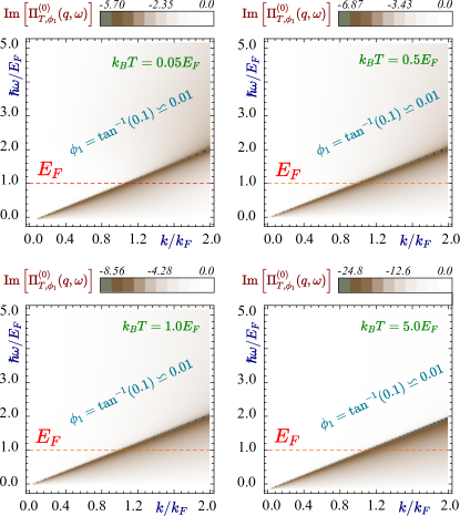
Figure 1: (Color online) Particle-hole modes, or single-particle excitation regions for an $\alpha-\mathcal{T}_{3}$ material with a small phase $\phi_{1}=\tan^{-1}(0.1)\backsim 0.01$. The particle-hole modes are obtained as the regions of non-zero $\text{Im}\,\Pi^{(0)}_{\phi,T}(q,\omega)$ so that each panel corresponds to a specific temperature ($0.05\,E_{F}/k_{B}$, $0.5\,E_{F}/k_{B}$ $1.0\,E_{F}/k_{B}$ and $5.0\,E_{F}/k_{B}$), as labeled. Completely white areas with $\text{Im}\,\Pi^{(0)}_{\phi,T}(q,\omega)=0$ outline the regions with damping-free excitations.

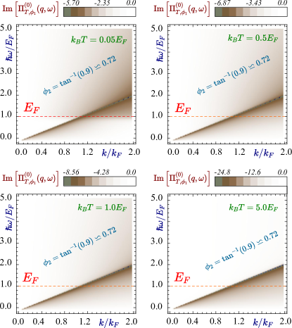
Figure 2: (Color online) Particle-hole modes, or single-particle excitation regions for an $\alpha-\mathcal{T}_{3}$ material with a large value of phase $\phi_{1}=\tan^{-1}(0.9)\backsim 0.73$. The particle-hole modes are obtained as the regions of non-zero $\text{Im}\,\Pi^{(0)}_{\phi,T}(q,\omega)$ so that each panel corresponds to a specific temperature ($0.05\,E_{F}/k_{B}$, $0.5\,E_{F}/k_{B}$ $1.0\,E_{F}/k_{B}$ and $5.0\,E_{F}/k_{B}$), as labeled. Completely white areas with $\text{Im}\,\Pi^{(0)}_{\phi,T}(q,\omega)=0$ outline the regions with damping-free excitations.

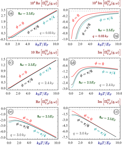
Figure 3: (Color online) Real (left panels) and imaginary (right panels) parts of polarization function as $\Pi^{(0)}_{\phi,T}(q,\omega)$ a function of temperature for various types of extrinsic (or doped) $\alpha-\mathcal{T}_{3}$ materials at specific points with a fixed frequency $\hbar\omega=2.5\,E_{F}$ for all panels, and the wave vector $q=0.03\,k_{F}$ (long-wave limit) for top panels $(a)$ and $(b)$, $q=2.4\,k_{F}$ for middle plots $(c)$ and $(d)$, and $q=3.0\,k_{F}$ for the lower panels $(e)$ and $(f)$. In each plot, red, black and blue curves correspond to $\phi=0$ (graphene), $\phi=\pi/6$ and $\phi=\pi/4$ (a dice lattice), as labeled.

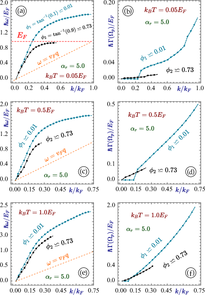
Figure 4: (Color online) Plasmon dispersions (left panels) and their damping rates (right panels) for $\alpha-\mathcal{T}_{3}$ materials at different temperatures. Top panels $(a)$ and $(b)$ describe the situation for a low temperature $k_{B}T=0.05\,E_{F}$, middle plots $(c)$ and $(d)$ - for $k_{B}T=0.5\,E_{F}$, and the lower panels $(e)$ and $(f)$ - for $k_{B}T=1.0\,E_{F}$. In each panel, a blue curve is related to a material with $\alpha=0.1$ (nearly graphene), while the black one - to $\alpha=0.9$ (nearly dice lattice). The relative dielectric constant is taken $\alpha_{r}=5.0$ for all cases.

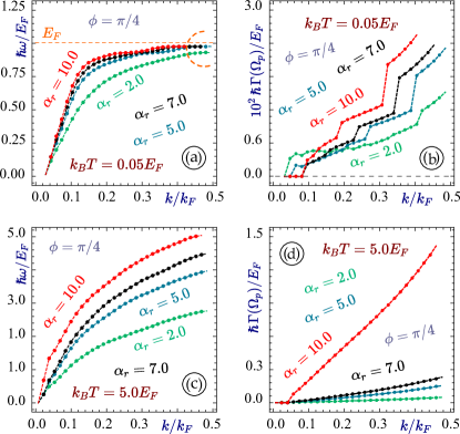
Figure 5: (Color online) The suppression of the so-called “plasmon pinching effect” in a dice lattice at finite temperature. Panel $(a)$ demonstrates the plasmon dispersions for a dice lattice ($\phi=\pi/4$) at or nearly zero temperature $k_{B}T=0.05\,E_{F}$ for different values of a dielectric constant $\alpha_{r}=2.5$, $5.0$, $7.0$ and $10.0$ so that all the branches intersect at $\hbar\omega=\hbar v_{F}q=E_{F}$. Similar plasmon dispersions at a large temperature $k_{B}T=5.0\,E_{F}$ are shown in plot $(c)$. The right panels $(b)$ and $(d)$ represent the corresponding damping rates.

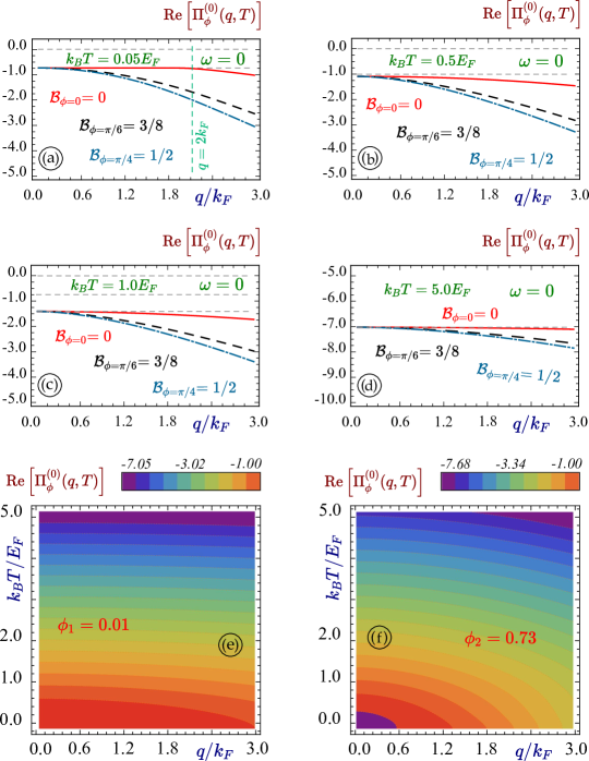
Figure 6: (Color online) Static limit of the real part polarization function $\Pi^{(0)}_{\phi,T}(q,\omega=0\,|\,\mu)$ (its imaginary part is zero) for different $\alpha-\mathcal{T}_{3}$ materials at a finite temperatures. Panels $(a)$ - $(d)$ show $\Pi^{(0)}_{\phi,T}(q,\omega=0\,|\,\mu)$ as a function of wavevector $q$ for $T=0.05\,E_{F}/k_{B}$, $0.5\,E_{F}/k_{B}$, $1.0\,E_{F}/k_{B}$ and $5.0\,E_{F}/k_{B}$, correspondingly. In each panel, the red blue and black curves are related to different phases ($\phi=0$, $\pi/6$ and $\pi/4$), as labeled. The two lower panels $(e)$ and $(f)$ demonstrate density plots of the $\Pi^{(0)}_{\phi,T}(q,\omega=0\,|\,\mu)$ as a function of the wave vector $q$ and temperature $T$ simultaneously for phase $\phi_{2}=\tan^{-1}(0.1)=0.01$ (nearly graphene) and $\phi_{2}=\tan^{-1}(0.9)\backsimeq 0.73$ (nearly a dice lattice).

III Long wavelength limit of $\Pi_{\phi,T}^{(0)}(q,\omega)$ at zero and finite temperatures

In this section, our aim is to find the long wavelength limit ($q\longrightarrow 0$) of the polarization function and the plasmon dispersions which are often used to evaluate a number of crucial properties of the material and the plasmon behavior in various heterostructures Gumbs et al. (2015); Iurov et al. (2017c) Our results for $T=0$ and $q\ll E_{F}/(\hbar v_{F})$ are based on analytical expressions for the polarization function demonstrated in Ref. [Malcolm and Nicol, 2016]. Strictly speaking, our results for an arbitrary $\alpha$-T₃ case is an interpolation (not a rigorous derivation): we presented the expressions for a dice lattice as the corresponding result for graphene plus additional non-graphene terms and interpolated these extra terms $\backsim\mathcal{B}_{\phi}=1/2\,\sin^{2}(2\phi)$ for all $\alpha-\mathcal{T}_{3}$ materials. However, we strongly believe that this result is precise because exactly the same $\phi-$dependence was rigorously obtained in our thorough static limit derivation in Section IV.

Following our derivation in Appendix B, we write

$$16\pi\hbar^{2}g^{-1}\,\Pi_{\phi}^{(0)}(q,\omega)=2E_{F}\left\{\frac{2}{\omega^{2}}-\frac{\mathcal{B}_{\phi}(\hbar\omega)^{2}}{\left[4E_{F}^{2}-(\hbar\omega)^{2}\right]^{2}}\right\}\,q^{2}-(1+6\mathcal{B}_{\phi})\,\frac{q^{2}}{\hbar\omega}\,\ln\left[\frac{2E_{F}+\hbar\omega}{2E_{F}-\hbar\omega}\right]\,.$$ (6)

Now we are assured that the plasmon branch varies as $\backsim\sqrt{q}$, as it should be for any two-dimensional Dirac cone lattice. This means that for $q\longrightarrow 0$, the plasmon is located at an energy $\Omega_{p}\backsim\sqrt{q}\ll E_{F}$ and Eq. (33) could be further simplified as

$$16\pi g^{-1}\,\text{Re}\,\Pi_{\phi,T=0}(q,\omega)=\left\{\frac{4E_{F}}{(\hbar\omega)^{2}}-\left(1+6\mathcal{B}_{\phi}\right)\frac{2}{E_{F}}-\mathcal{B}_{\phi}\frac{(\hbar\omega)^{2}}{(2E_{F})^{3}}\right\}\,q^{2}\,.$$ (7)

The analytical expression for the real part of the zero-temperature polarization function could be found only for finite and sufficiently large doping level $E_{F}$. The polarization function for finite doping cannot be presented as intrinsic $\text{Re}\,\Pi_{\phi,T=0}(q,\omega)$ plus an additional term proportional to the Fermi energy. Therefore, the integral transformation in Eq.  (3) cannot be applied to the real part of the polarization function 7 and the analytical expression for the temperature-induced modification of the polarization function needs to be generalized in the presence of a flat band. We would, however, estimate the finite-temperature real polarizability using the fact that at $T=0$ K the flat band has only very limited effect on the polarization function (next order of $\hbar\omega$) and the plasmon branch in the long wavelength limit. Apart from that, at high temperature $k_{B}T\gg E_{F}$ and the long wavelength limit $q\ll k_{F}$ the situation is such that the finite electron doping $E_{F}$ has a negligible effect on the polarization function and the plasmon branch, Sarma and Li (2013) i.e., at high temperature the extrinsic and intrinsic materials’ behavior is almost identical. Therefore, in the lowest-order approximation, we can assume that the polarization function is the same as for undoped graphene. Sarma and Li (2013)

$$\text{Re}\,\Pi_{\phi,T\gg E_{F}}(q,\omega)=\frac{g\ln 2}{2\pi}\,k_{B}T\,\frac{q^{2}}{\omega^{2}}\,$$ (8)

In the lowest order for which a coefficient $\mathcal{B}_{\phi}=1/2\sin^{2}(2\phi)$ would not vanish, the zero-temperature plasmon branch for an $\alpha-\mathcal{T}_{3}$ lattice is given as

$$\Omega_{p}^{2}(q,T=0\,|\,E_{F},\phi)=\frac{2gE_{F}^{2}\,q}{4E_{F}+g\left(1+6\mathcal{B}_{\phi}\right)\,q}\backsimeq\frac{gE_{F}}{2\hbar^{2}}\,q-\left(1+6\mathcal{B}_{\phi}\right)\frac{g^{2}}{8\hbar^{2}}\,q^{2}+...\,.$$ (9)

The imaginary part of the polarization function for an $\alpha-\mathcal{T}_{3}$ model is calculated as (see Appendix B)

$$\text{Im}\,\Pi^{(0)}_{\phi,T=0}(q,\omega)\backsimeq-\frac{g\,q^{2}}{16\,\hbar\omega}\Big{\{}4\mathcal{B}_{\phi}\Theta(\omega-E_{F})+(1-2\mathcal{B}_{\phi})\,\Theta\left[\omega-2E_{F}\right]\Big{\}}\,.$$ (10)

The imaginary part of the finite-temperature polarization function in Eq. (10) could be easily calculated as

$$\text{Im}\,\Pi^{(0)}_{\phi,T\gg T_{F}}(q,\omega\,|\,\mu)\backsimeq\frac{g}{16}\,\frac{q^{2}}{\hbar\omega}\,\left\{4\mathcal{B}_{\phi}\,\tanh\left(\frac{\omega-\mu}{2k_{B}T}\right)+(1-2\mathcal{B}_{\phi})\,\tanh\left[\frac{\omega-2\mu}{4k_{B}T}\right]+(1+2\mathcal{B}_{\phi})\,\tanh\left[\frac{\mu}{2k_{B}T}\right]\right\}\,.$$ (11)

At high temperature $k_{B}T\gg\mu$ or $k_{B}T\gg\omega$, we can approximate $\tanh x\backsimeq x$ so that

$$\text{Im}\,\Pi^{(0)}_{\phi,T\gg T_{F}}(q,\omega\,|\,\mu)\backsimeq-\frac{g}{64}\,\frac{q^{2}}{k_{B}T}\,\left(1+6\mathcal{B}_{\phi}\right)\,.$$ (12)

The effect of doping on the imaginary part of the polarizability is only seen in the next-order corrections:

$$\text{Im}\,\Pi^{(0)}_{\phi,T\gg T_{F}}(q,\omega\,|\,\mu)\backsimeq-\frac{g}{64}\,\frac{q^{2}}{k_{B}T}\,\left\{1-\frac{1}{48}\,\left(\frac{\omega}{k_{B}T}\right)^{2}+6\mathcal{B}_{\phi}\,\left[1-\frac{5}{48}\,\left(\frac{\omega}{k_{B}T}\right)^{2}\right]\right\}\,.$$ (13)

Here, we assumed that at high temperature $k_{B}T\gg E_{F}$ we can use $\omega\backsim k_{B}T\gg\mu(T)$.

The decay rate $\Gamma_{\phi,T}[q,\Omega_{p}(q)\,|\,\mu]$ of the obtained plasmon branches for the case of low damping could be approximated in the first order of $\Gamma(q,\Omega_{p})/\Omega_{p}(q)$ as

$$\Gamma_{\phi,T}[q,\Omega_{p}(q)\,|\,\mu]=\text{Im}\,\Pi^{(0)}_{\phi,T}(q,\omega\,|\,\mu)\,\left\{\frac{\partial}{\partial\omega}\text{Re}\,\Pi^{(0)}_{\phi,T}(q,\omega\,|\,\mu)\Big{|}_{\omega=\Omega_{p}(q)}\right\}^{-1}\,.$$ (14)

Such an approximation works particularly well at a large temperature $k_{B}T\gg E_{F}$ and a small wave vector $q\ll k_{F}$ when the real part grows $\backsim T$ and imaginary part is reduced as $\backsim 1/T$. For the intermediate part, the validity of approximation 14 is not obvious and must be verified by the effect of the next-order terms $\backsim\Gamma^{2}$ etc.

Substituting the obtained expressions (8) and (12) for the high-temperature limit of the real and imaginary parts of the polarization function into the plasmon equation (2), we obtained the thermal plasmon dispersions and their damping rates is

$$\Omega_{p}(q,T)=\sqrt{\alpha_{r}g\log(2)\,\hbar v_{F}q\,k_{B}T}\,,$$ (15)

$$\Gamma_{\phi,T}[q,\Omega_{p}(q)]=\frac{g\pi}{32}\,\sqrt{\log(2)}\,\frac{(\alpha_{r}\,\hbar v_{F}q)^{3/2}}{\sqrt{k_{B}T}}\,\left(1+6\mathcal{B}_{\phi}\right)\,.$$

Qualitatively, the behavior of the high-temperature plasmons in $\alpha-\mathcal{T}_{3}$ and in a dice lattice is similar to graphene.

The particle-hole mode region, corresponding to finite imaginary part of the polarization function, for different $\alpha-\mathcal{T}_{3}$ at finite temperatures, are presented at Figs. 1 and 2. We observe that $\text{Im}\,\Pi^{(0)}_{\phi,T}(q,\omega\,|\,\mu)$ is increasing with temperature for sufficiently large values of the wave vector $q$ which is opposite to its behavior for $q\to 0$. In the long wavelength limit, the imaginary part of the polarization function drops exactly as $\backsim 1/T$ which is especially well demonstrated at high temperatures (see Eqs (15) and (12)). Once the temperature becomes finite, we no longer see a clear division of the areas with zero and non-zero polarization function which define the areas of undamped plasmons and the single-particle excitation spectrum. The largest values of imaginary polarization is observed along the main diagonal $\omega=v_{F}q$ for all temperatures.

The real part of the polarization function, presented in Fig. 3 increases nearly proportional with the temperature. However, it could be either positive or negative depending on its location relative to the main diagonal. Both real and imaginary parts of $\Pi^{(0)}_{\phi,T}(q,\omega\,|\,\mu)$ for any $\alpha>0$ are bigger than for graphene, and their values monotonically increase with increasing phase $\phi$ due to the fact that if the flat band is present more transitions from and to the flat band have to be taken into account, and the weight of this contributing term keeps monotonically increasing with phase $\phi$.

Plasmon damping rates for various, calculations using Eq. (14) for $\alpha-\mathcal{T}_{3}$ materials and different temperatures are shown in Fig. 4. Generally, the damping rate is affected by phase $\phi$ (the effect of the presence of the flat band) a lot more than the actual plasmon dispersions $\Omega_{p}(q)$. In the long wavelength limit, we see that the dispersions of the plasmon branches only decrease in the second order of $q$. For larger wave vectors $q$, this decrease becomes more substantial, but the most important difference is between a dice lattice (and any $\alpha-\mathcal{T}_{3}$ with $\alpha>0$) and graphene is the strong damping at low frequencies $\hbar\omega\backsimeq E_{F}$ which makes the plasmon branch strongly damped at any temperature.

At high temperature, the plasmon branches corresponding to phases $\phi_{1}$ (almost graphene) and $\phi_{2}$ (almost a dice lattice) are located closer to each other meaning that the effect of the flat band is largely suppressed, but for a large phase the plasmons become highly damned at lower frequencies irrespective of the temperature. The decay rate of the plasmons is also strongly affected by the $\omega$- derivative, or how closely the branch is located to the main diagonal $\omega=v_{F}q$. Thus, we see that for graphene-like materials the damping is stronger for small wave vector values (black curves in Figure 4.

Additionally, it seems interesting to investigate the so-called plasmon pinching effect meaning that all the plasmon dispersions corresponding to different relative dielectric constants $\alpha_{r}$ intersect at $\hbar\omega=\hbar v_{F}q=E_{F}$. We see that at finite temperature this effect no longer exists, and the plasma branches are well separated, as well as the corresponding damping rates. The plasmon branches for the smaller values of $\alpha_{r}$ are located at lower frequencies closer to the main diagonal which increases the $\omega$-derivative of the real part of the polarization function.

IV Static limit of the polarization function

We now turn our attention to the calculation of a static ($\omega=0$) limit of the polarization function $\Pi_{0,\phi}(q,T)$ for $\alpha-\mathcal{T}_{3}$ materials with arbitrary $0<\alpha<1$ and finite temperature $T$. The obtained function also referred to as the Lindhard function must be real for all wave vectors $q$ since $q>\omega=0$ and $\omega<\mu(T)$ conditions are always satisfied.

As we demonstrate in Appendix C, the zero-frequency electron polarization function can be written as

$$\Pi_{\phi}^{(0)}(q,T)=\frac{g}{2\pi}\,\frac{1}{(\hbar v_{F})^{2}}\,\left\{\chi^{(+)}_{\phi}(q,T)+\chi^{(0)}_{\phi}(q,T)+\chi^{(-)}_{\phi}(q,T)\right\}\,,$$ (16)

where

$$\,\chi^{(+)}_{\phi}(q,T)=-\mu(T)-k_{B}T\,\log\left\{1+\texttt{exp}\left[\frac{-\mu}{k_{B}T}\right]\right\}+\hbar v_{F}\int\limits_{0}^{q/2}\frac{dk\,\left[1+2\mathcal{B}_{\phi}-(2k/q)^{2}\right]}{\left[1+\texttt{exp}\left\{[\varepsilon(k)-\mu]/(k_{B}T)\right\}\right]\,\sqrt{1-(2k/q)^{2}}}$$ (17)

$$+2\hbar v_{F}\mathcal{B}_{\phi}\int\limits_{0}^{q/2}\,\frac{dk\,[q/(2k)]^{2}}{1+\texttt{exp}\left\{[\varepsilon(k)-\mu]/(k_{B}T)\right\}}\,\left\{1-\left[1-(2k/q)^{2}\right]^{-1/2}\right\}+2\hbar v_{F}\mathcal{B}_{\phi}\int\limits_{q/2}^{\infty}dk\,\left(\frac{q}{2k}\right)^{2}\,\left\{1+\texttt{exp}\left[\frac{\hbar v_{F}k-\mu}{k_{B}T}\right]\right\}^{-1}\,,$$

$$\,\chi^{(-)}_{\phi}(q,T)=-(1+4\mathcal{B}_{\phi})\frac{\pi}{8}\,\hbar v_{F}q-k_{B}T\,\log\left\{1+\texttt{exp}\left[\frac{-\mu}{k_{B}T}\right]\right\}+\hbar v_{F}\int\limits_{0}^{q/2}\frac{dk\,\left[1+2\mathcal{B}_{\phi}-(2k/q)^{2}\right]}{\left[1+\texttt{exp}\left\{[\varepsilon(k)+\mu]/(k_{B}T)\right\}\right]\,\sqrt{1-(2k/q)^{2}}}$$

$$+2\hbar v_{F}\mathcal{B}_{\phi}\int\limits_{0}^{q/2}\,\frac{dk\,[q/(2k)]^{2}}{1+\texttt{exp}\left\{[\varepsilon(k)+\mu]/(k_{B}T)\right\}}\,\left\{1-\left[1-(2k/q)^{2}\right]^{-1/2}\right\}+2\hbar v_{F}\mathcal{B}_{\phi}\int\limits_{q/2}^{\infty}dk\,\left(\frac{q}{2k}\right)^{2}\,\left\{1+\texttt{exp}\left[\frac{\hbar v_{F}k+\mu}{k_{B}T}\right]\right\}^{-1}\,,$$

and

$$\chi^{(0)}_{\phi}(q,T)=0\,$$ (18)

represent three contributing terms with the conduction, valence and flat band types of the Fermi-Dirac distribution function $f(\gamma,k)=\left\{1+\texttt{exp}[(\gamma\hbar v_{F}k-\mu)/(k_{B}T)]\right\}^{-1}$, where $\gamma=\pm 1$ and $0$.

At zero temperature, an exact analytical formula could be obtained

$$\,\chi^{(+)}_{\phi}(q,T\rightarrow 0)=-E_{F}+(1+4\mathcal{B}_{\phi})\frac{\pi}{8}\,\hbar v_{F}q-\mathcal{B}_{\phi}\frac{(\hbar v_{F}q)^{2}}{2E_{F}}\,,$$ (19)

for $q<2k_{F}$ and

$$\chi^{(+)}_{\phi}(q,T\rightarrow 0)= -E_{F}+\frac{E_{F}}{2}\sqrt{1-\left(\frac{2k_{F}}{q}\right)^{2}}+\hbar v_{F}q\,\left(\frac{1}{4}+\mathcal{B}_{\phi}\right)\,\arcsin\left(\frac{2k_{F}}{q}\right)$$

$$-\mathcal{B}_{\phi}\frac{(\hbar v_{F}q)^{2}}{2E_{F}}\left[1-\sqrt{1-\left(\frac{2k_{F}}{q}\right)^{2}}\,\right]\,$$

for $q>2k_{F}$. Thus, $\chi^{(+)}_{\phi}(q,T)$ could be presented by a single unified expression

$$\chi^{(+)}_{\phi}(q,T\rightarrow 0)= -E_{F}+(1+4\mathcal{B}_{\phi})\frac{\pi}{8}\,\hbar v_{F}q-\mathcal{B}_{\phi}\frac{(\hbar v_{F}q)^{2}}{2E_{F}}+\left\{\frac{1}{2}\,\left(E_{F}+\mathcal{B}_{\phi}\,\frac{q^{2}}{E_{F}}\right)\sqrt{1-\left(\frac{2k_{F}}{q}\right)^{2}}\right.$$

$$-\left.\hbar v_{F}q\,\left[\frac{1}{4}+\mathcal{B}_{\phi}\right]\,\arccos\left(\frac{2k_{F}}{q}\right)\,\right\}\,\Theta(q-2k_{F})\,.$$

The hole contribution term $\chi^{(-)}_{\phi}(q,T)$ at $T\rightarrow 0$ becomes

$$\,\chi^{(-)}_{\phi}(q,T\rightarrow 0)=-(1+4\mathcal{B}_{\phi})\frac{\pi}{8}\,\hbar v_{F}q\,,$$ (22)

which for a dice lattice with $\mathcal{B}_{\phi}=1/2$ exactly matches the corresponding results of Ref. [Malcolm and Nicol, 2016].

We plot the results for the finite-temperature static polarizability in Fig. 6. The main difference between graphene and $\alpha-\mathcal{T}_{3}$ is a smooth variation of the Lindhard function around $q=2k_{F}$ for all $\alpha\neq 0$ which means a lower order for the Thomas-Fermi decay not only for a dice lattice but for all other $\alpha-\mathcal{T}_{3}$ lattices. Apart from that, the $q$-dependence of the static polarization function is smooth for any non-zero temperature regardless of of the phase $\phi$.

We have observed that the Lindhard function for any $\alpha>0$ exceeds that for graphene and it always increases with the phase $\phi$ for both zero and finite temperatures since for a finite $\phi$ more electron transitions with a larger weight contribute to the sum in Eq. (3). There is also a substantial increase of $\Pi_{\phi}^{(0)}(q,T)$ with rising temperature which is a lot more noticeable than its $q-$ dependence. The finite-temperature static dielectric function $\epsilon(q,T)$ is the central quantity for calculating the Boltzmann conductivity in a wide class of pseudospin-1 Dirac materials.

V Concluding remarks and Summary

In this work, we have investigated the polarization function, plasmons and their damping rates in $\alpha-\mathcal{T}_{3}$ materials. The calculations were carried out at finite temperature with the main focus on the temperature dependence of the effect of the presence of a flat band in the electron bandstructure.

The particle-hole modes, determined by the finite imaginary part of the polarization function, demonstrate completely different behaviors dependent on their location in the $(q,\omega)$-plane. In the long wavelength limit, the high-temperature behavior of the plasmon and its damping is qualitatively similar to graphene, i.e., $\text{Im}\,\Pi^{(0)}_{\phi,T\gg T_{F}}(q,\omega\,|\,\mu)$ falls off on $1/T$. On the other hand, the real part of the polarization function increases as $\backsim T$ so that the plasmon is well defined as long as $k_{B}T/\gg E_{F}$. However, the actual values of $\text{Im}\,\Pi^{(0)}_{\phi,T\gg T_{F}}(q,\omega\,|\,\mu)$ and $\Gamma_{\phi,T}[q,\Omega_{p}(q)]$ differing substantially from that in graphene being significantly larger at any finite temperature.

We have obtained a closed-form analytical expression for the long wavelength limit of the polarization function and plasmon dispersions for all $\alpha-\mathcal{T}_{3}$ materials. Additionally, we have demonstrated that this long wavelength behavior is nearly similar to the case of graphene $(\phi=0)$ and the effect of the flat band is only revealed in the next order in $q$ as $\backsim q^{2}$. The plasmon pinching effect is suppressed at any finite temperature so that the plasmon branches corresponding to different dielectric constants $\alpha_{r}$ would no longer intersect at one point. We have also obtained semi-analytical expressions for the Lindhard function, or the static limit of the polarization function. These results were obtained for various temperatures with completely analytical approximations for the high, low and zero temperatures for an arbitrary $\alpha-\mathcal{T}_{3}$ material with $0<\alpha<1$.

The static polarization function is of special importance and is is often highlighted for the role it plays in collective phenomena. This is so because the static dielectric function is the key component for the temperature-dependent conductivity in the presence of charged impurities, finite-temperature screening and, more generally, Boltzmann transport. It is also employed in evaluating the screened potential of a point charge, Friedel oscillations and the effect of an electric or magnetic impurity on the electron response, as well as the RKKY interaction. Our convenient, handy and ready-to-use semi-analytical expressions are expected to motivate researchers leading to a new wave of research of the many-body properties of $\alpha-\mathcal{T}_{3}$ materials.

In brief, we have discovered some important information on the plasmons and collective behavior of pseudospin-1 Dirac materials at finite temperatures. We are confident that these results will find numerous applications in both fundamental research of these innovative systems and their applications. Specifically, we believe that our crucial analytical expressions will be useful to experimentalists for predicting the behavior of flat-band materials at experimentally accessible high and room temperatures.

VI Acknowledgments

AI would like to acknowledge the funding provided by TRADA-52-113 PSC-CUNY Award No. 64076-00 52. DH would like to acknowledge the financial supports from Air Force Office of Scientific Research (AFOSR). GG would like to acknowledge the support from Air Force Research Laboratory (AFRL) through Contract $\#$ FA9453-18-1-0100.

Appendix A Finite-temperature polarization function - miscellaneous derivations

A.1 Finite-temperature polarization function $\Pi^{(0)}_{\phi,T}(q,\omega\,|\,\mu)$

We first demonstrate that the finite-temperature polarization function $\Pi^{(0)}_{\phi,T}(q,\omega\,|\,\mu)$ could be obtained as a straightforward integral transformation of its zero-temperature counterpart. The validity of Eq. (3) is based on the assumption that all the quantities in Eq. (4) except the Fermi-Dirac distribution functions $n_{F}[\gamma\epsilon(k),T]$ are temperature independent and, therefore, the main idea of our derivation is to prove that $n_{F}[\gamma\epsilon(k),T]$ is obtained from its zero-temperature counterpart $n_{F}[\gamma\epsilon(k),T=0]=\Theta[E_{F}-\gamma\epsilon(k)]$ by applying the exactly identical convolution in Eq. (3)  Maldague (1978); Iurov et al. (2016, 2020d)

$$n_{F}[\epsilon(k),T]=\int\limits_{-\infty}^{\infty}d\eta\,\frac{\Theta[\nu-\epsilon(k)]}{4k_{B}T}\cosh^{-2}\left\{\frac{\eta-\mu(T)}{2k_{B}T}\right\}=\int\limits_{\gamma\epsilon(k)}^{\infty}\frac{d\eta}{4k_{B}T}\cosh^{-2}\left\{\frac{\nu-\mu(T)}{2k_{B}T}\right\}\,.$$ (23)

Integral (23) could be easily carried out yielding

$$\int\limits_{\gamma\epsilon(k)}^{\infty}\frac{d\eta}{4k_{B}T}\cosh^{-2}\left[\frac{\eta-\mu(T)}{2k_{B}T}\right]=\frac{1}{2}\,\tanh\left[\frac{\eta-\mu(T)}{2k_{B}T}\right]\Bigg{|}_{\gamma\epsilon(k)}^{\infty}=\frac{1}{2}\left\{1-\tanh\left[\frac{\epsilon(k)-\mu(T)}{2k_{B}T}\right]\right\}\,.$$ (24)

On the other hand, the Fermi-Dirac function could be presented as

$$n_{F}(\xi)=-\tanh\left(\frac{\xi}{2}\right)+n_{F}(-\xi)$$ (25)

or

$$2n_{F}(\xi)=-\tanh\left(\frac{\xi}{2}\right)+1\,,$$ (26)

where $\xi=[\epsilon(k)-\mu(T)]/(2k_{B}T)$. Substituting expression (26) into Eq. (24) immediately verifies our statement.

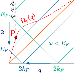
Figure 7: (Color online) Illustration for calculating the finite-temperature polarization function $\Pi^{(0)}_{\phi,T}[q,\omega\,|\,\mu(T)]$ by Eq. (3) as an integral over a variable chemical potential $\eta$.

For the hole states with $\gamma=-1$ and $\gamma\epsilon(k)<0$, the Fermi-Dirac distribution functions are presented as $n_{F}[-\epsilon(k)-\mu(T)]=1-n_{F}[\epsilon(k)+\mu(T)]$ and a similar type of transformations could be performed. The undoped part of the polarization function does not depend on temperature:

$$\Pi^{(0)}_{\phi,T}(q,\omega\,|\,\mu=0)=\frac{1}{4k_{B}T}\int\limits_{-\infty}^{\infty}\frac{d\eta}{\pm[\epsilon(k)+\epsilon(k^{\prime})]+\hbar\left(\omega+i0^{+}\right)}\,\cosh^{-2}\left\{\frac{\eta-0}{2k_{B}T}\right\}=\Pi^{(0)}_{\phi,T=0}(q,\omega\,|\,E_{F}=0)\,,$$ (27)

i.e., the finite-temperature undoped polarizability is obtained by the same integral transformation Eq. (3), and exactly the same reasoning could be applied to the transitions from and to the flat band with $\gamma=0$ and $\epsilon(k)\equiv 0$.

Appendix B Long wavelength limit $q\longrightarrow 0$ for the polarization function

B.1 Real part of the polarization function $\text{Im}\,\Pi^{(0)}_{\phi,T=0}(q,\omega)$

In the region of interest ($R_{2}$ and $R_{4}$ defined in Fig. 8), the polarization function for a dice lattice is obtained as  Malcolm and Nicol (2016)

$$-\Pi_{\phi}^{(0)}(q,\omega)=\frac{g}{2\pi}\,E_{F}+\frac{g}{16\pi}\,\left[\omega+\frac{q^{2}}{\omega}\right]\ln X\big{|}_{X=r_{1}}^{X=s_{1}}+\frac{g}{16\pi}\,\big{[}\mathbb{G}^{(0)}_{q}(X)+\mathbb{D}^{(\phi)}_{q}(X)\big{]}\big{|}_{X=r}^{X=s}\,,$$ (28)

where $\{s,r\}=2E_{F}\pm\omega$ and $\{s_{1},r_{1}\}=E_{F}\pm\omega$. The two functions

$$\mathbb{G}^{(0)}_{q}(X)=-X\sqrt{\frac{X^{2}-q^{2}}{\omega^{2}-q^{2}}}+\frac{q^{2}}{\sqrt{\omega^{2}-q^{2}}}\,\ln\left[(X+\sqrt{X^{2}-q^{2}}\,)/q\right]\,,$$ (29)

$$\mathbb{D}^{(\phi)}_{q}(X)=-2\sqrt{\omega^{2}-q^{2}}\,\ln\left[(X+\sqrt{X^{2}-q^{2}}\,)/q\right]+\left[\omega+\frac{q^{2}}{\omega}\right]\,\ln\left\{\frac{\omega\sqrt{X^{2}-q^{2}}+(\omega\leftrightarrow X)}{\omega\sqrt{X^{2}-q^{2}}-(\omega\leftrightarrow X)}\right\}$$

correspond to graphene and additional terms obtained for a dice lattice. Here, $(\omega\leftrightarrow X)$ means double variable replacement which results in $X\sqrt{\omega^{2}-q^{2}}$ term.

For a general $\alpha-\mathcal{T}_{3}$ model, the equation could be extrapolated as

$$-\Pi_{\phi}^{(0)}(q,\omega)=\frac{g}{2\pi}\,E_{F}+2\mathcal{B}_{\phi}\,\frac{g}{16\pi}\,\left[\omega+\frac{q^{2}}{\omega}\right]\ln X\big{|}_{X=r_{1}}^{X=s_{1}}+\frac{g}{16\pi}\,\big{[}\mathbb{G}_{q}(X)+2\mathcal{B}_{\phi}\,\mathbb{F}_{q}(X)\big{]}\big{|}_{X=r}^{X=s}\,,$$ (30)

At this point, we are in a position to obtain the long wavelength approximation of the polarization function. Calculation shows that

$$\mathbb{G}^{(0)}_{q\longrightarrow 0}(s)-\mathbb{G}^{(0)}_{q\longrightarrow 0}(r)\backsimeq -8E_{F}-\frac{4E_{F}}{\omega^{2}}\,q^{2}+\frac{q^{2}}{\omega}\left\{\ln\left[\frac{2E_{F}+\omega}{2E_{F}-\omega}\right]+\frac{q^{2}}{2}\,\frac{\omega E_{F}}{\left(4E_{F}^{2}-\omega^{2}\right)^{2}}\right\}\,$$ (31)

$$\backsimeq -8E_{F}-\frac{q^{2}}{\omega}\left\{\frac{4E_{F}}{\omega}-\ln\left[\frac{2E_{F}+\omega}{2E_{F}-\omega}\right]\right\}+...\,.$$

$$\mathbb{D}^{(\phi)}_{q\longrightarrow 0}(s)-\mathbb{D}^{(\phi)}_{q\longrightarrow 0}(r)\backsimeq -\left(2\omega-\frac{q^{2}}{\omega}\right)\left\{\ln\left[\frac{2E_{F}+\omega}{2E_{F}-\omega}\right]+\frac{q^{2}}{2}\,\frac{\omega E_{F}}{\left(4E_{F}^{2}-\omega^{2}\right)^{2}}\right\}$$

$$+\left(\omega+\frac{q^{2}}{\omega}\right)\left\{\ln\left[\frac{(2E_{F}+\omega)^{2}(E_{F}-\omega)}{(2E_{F}-\omega)^{2}(E_{F}+\omega)}\right]+\frac{2E_{F}\omega\,q^{2}}{(4E_{F}^{2}-\omega^{2})^{2}}\right\}+...\backsim$$

$$\backsimeq\omega\ln\left[\frac{E_{F}-\omega}{E_{F}+\omega}\right]+\frac{\omega^{2}E_{F}\,q^{2}}{\left(4E_{F}^{2}-\omega^{2}\right)^{2}}+\frac{q^{2}}{\omega}\,\ln\left[\frac{(2E_{F}+\omega)^{3}(E_{F}-\omega)}{(2E_{F}-\omega)^{3}(E_{F}+\omega)}\right]+...\,.$$

Consequently, the polarization function for the long-wave limit $q\rightarrow 0$ is given by

$$16\pi\hbar^{2}g^{-1}\,\Pi_{\phi}^{(0)}(q,\omega)=2E_{F}\left\{\frac{2}{\omega^{2}}-\frac{\mathcal{B}_{\phi}\omega^{2}}{\left(4E_{F}^{2}-\omega^{2}\right)^{2}}\right\}\,q^{2}+(1+6\mathcal{B}_{\phi})\,\frac{q^{2}}{\omega}\,\ln\left[\frac{2E_{F}-\omega}{2E_{F}+\omega}\right]\,.$$ (33)

Including all the relevant constants, we rewrite the final expression as

$$16\pi\hbar^{2}g^{-1}\,\Pi_{\phi}^{(0)}(q,\omega)=2E_{F}\left\{\frac{2}{\omega^{2}}-\frac{\mathcal{B}_{\phi}(\hbar\omega)^{2}}{\left[4E_{F}^{2}-(\hbar\omega)^{2}\right]^{2}}\right\}\,q^{2}-(1+6\mathcal{B}_{\phi})\,\frac{q^{2}}{\hbar\omega}\,\ln\left[\frac{2E_{F}+\hbar\omega}{2E_{F}-\hbar\omega}\right]\,.$$ (34)

We are now assured that the plasmon dispersion varies as $\backsim\sqrt{q}$, as it should be for any two-dimensional Dirac cone lattice. This means that for $q\longrightarrow 0$, the plasmon is located at an energy $\Omega_{p}\backsim\sqrt{q}\ll E_{F}$ and Eq. (33) could be further simplified as

$$16\pi g^{-1}\,\Pi_{\phi}^{(0)}(q,\omega)=\left\{\frac{4E_{F}}{(\hbar\omega)^{2}}-\left(1+6\mathcal{B}_{\phi}\right)\frac{2}{E_{F}}-\mathcal{B}_{\phi}\frac{(\hbar\omega)^{2}}{(2E_{F})^{3}}\right\}\,q^{2}\,.$$ (35)

Obviously, this results is valid only for a finite and sufficiently large doping level $E_{F}$.

B.2 Imaginary part of the polarization function $\text{Im}\,\Pi^{(0)}_{\phi,T=0}(q,\omega)$

We begin our consideration with the imaginary part of the polarization function for a dice lattice for $q\longrightarrow 0$, i,e, in regions $R_{1}$, $R_{2}$ and $R_{4}$ assigned in Fig. 8:

$$\text{R}_{1}=\Theta(E_{F}-\omega)\,,$$ (36)

$$\text{R}_{2}=\Theta(\omega-E_{F})\,\Theta\left(E_{F}-\frac{\omega+q}{2}\right)\,,$$

$$\text{R}_{3}=\Theta\left(q-|\omega-2E_{F}|\right)\,\,\text{or}\,\,2E_{F}-q<\omega>2E_{F}+q,$$

$$\text{R}_{4}=\Theta\left(\frac{\omega-q}{2}-E_{F}\right)\,\,\text{or}\,\,\omega>2E_{F}+q\,.$$

Figure 8: (Color online) Schematic graph for the regions with different expressions for the polarization function for $q\longrightarrow 0$.

We exclude a small region $R_{3}$ According to Ref. [Malcolm and Nicol, 2016], the polarization function in the regions of interest is given as

$$-\text{Im}\,\Pi^{(0)}_{\phi,T=0}(q,\omega)=\frac{q^{2}}{2\omega}\,\Theta(\omega-E_{F})+\Theta\left(\frac{\omega-q}{2}-E_{F}\right)\left[\frac{q^{2}}{4\sqrt{\omega^{2}-q^{2}}}-\frac{1}{2}\sqrt{\omega^{2}-q^{2}}+\frac{\omega^{2}-q^{2}}{2\omega}\right]$$ (37)

In the long wavelength limit $q\longrightarrow 0$, Eq. (37) could be approximated as

$$-\text{Im}\,\Pi^{(0)}_{\phi,T=0}(q,\omega)=\frac{q^{2}}{2\omega}\,\Theta(\omega-E_{F})+\Theta\left(\frac{\omega-q}{2}-E_{F}\right)\frac{3q^{4}}{16\omega^{3}}$$ (38)

For a general $\alpha-\mathcal{T}_{3}$ lattice, we can only interpolate the known results for graphene and a dice lattice using a coefficient $\mathcal{B}_{\phi}=1/2\sin^{2}(2\phi)$

$$-\text{Im}\,\Pi^{(0)}_{\phi,T=0}(q,\omega)=\mathcal{B}_{\phi}\,\frac{q^{2}}{\omega}\,\Theta(\omega-E_{F})+\Theta\left(\frac{\omega-q}{2}-E_{F}\right)\left[\frac{q^{2}}{4\sqrt{\omega^{2}-q^{2}}}-\frac{\mathcal{B}_{\phi}}{2}\sqrt{\omega^{2}-q^{2}}+2\mathcal{B}_{\phi}\frac{\omega^{2}-q^{2}}{2\omega}\right]$$ (39)

Finally, in the long wavelength limit we obtain

$$\text{Im}\,\Pi^{(0)}_{\phi,T=0}(q,\omega)=-\mathcal{B}_{\phi}\,\frac{(\hbar v_{F}q)^{2}}{\omega}\,\Theta(\omega-E_{F})+\Theta\left[\frac{\omega-q}{2}-E_{F}\right]\left\{\frac{1-2\mathcal{B}_{\phi}}{4\omega}(\hbar v_{F}q)^{2}+\frac{1+\mathcal{B}_{\phi}}{16\omega^{3}}(\hbar v_{F}q)^{4}+...\right\}\backsimeq$$

$$\backsimeq-\frac{g\,q^{2}}{16\,\hbar\omega}\left\{4\mathcal{B}_{\phi}\Theta(\omega-E_{F})+(1-2\mathcal{B}_{\phi})\,\Theta\left[\frac{\omega-q}{2}-E_{F}\right]\right\}\,.$$ (40)

We did not include a narrow triangular region $R_{3}$ where $2E_{F}-q<\omega>2E_{F}+q$ into our consideration since for the finite temperature integral $\int\limits_{(\omega-q)/2}^{(\omega+q)/2}\,d\eta$ cannot affect the leading $\backsim q^{2}$ order of the finite-temperature polarization function. Similarly, we can make a modification $\Theta\left[\omega-q-2E_{F}\right]\rightarrow\Theta\left[\omega-2E_{F}\right]$ in Eq. (40).

Appendix C Lindhard function, static limit of the polarization function

The purpose of the present Appendix is to present a detailed derivation of the static limit of the polarization function $\Pi_{0}(q,\omega=0\,|\,\phi,\mu(T))$ for an $\alpha-\mathcal{T}_{3}$ material with any $0<\phi<\pi/4$ at an arbitrary finite temperature. For the static limit $\omega=0$, Eq. (4) is reduced to

$$\Pi_{0}(q,T)=\frac{g}{4\pi^{2}}\,\int d^{2}{\bf k}\sum\limits_{\gamma,\gamma^{\prime}=0\,\pm 1}\,\mathbb{O}_{\gamma_{1},\gamma_{2}}(\beta_{{\bf k},{\bf k}^{\prime}})\,\frac{n_{F}[\gamma,\epsilon(k)]-n_{F}[\gamma^{\prime},\epsilon(|{\bf k}^{\prime}|)]}{\epsilon_{\gamma}(k)-\epsilon_{\gamma^{\prime}}(|{\bf k}+\bf{q}|)}\,,$$ (41)

where ${\bf k}^{\prime}={\bf k}+{\bf q}$, $\epsilon_{\gamma}(k)=\gamma\epsilon(k)=\gamma\,\hbar v_{F}k$, $n_{F}[\gamma,\epsilon(k)]=n_{F}[\epsilon_{\gamma}(k),\mu]=\left\{1+\texttt{exp}[(\gamma\,\hbar v_{F}k-\mu)/(k_{B}T)]\right\}^{-1}$ is a short-hand notation for the distribution functions and $\mathbb{O}_{\gamma_{1},\gamma_{2}}(\beta_{{\bf k},{\bf k}^{\prime}})$ are the wave function overlaps given by Eq. (II).

Summation over $\gamma$ and $\gamma^{\prime}=-1,0,1$ results in

$$\Pi_{0}(q,T)=\frac{g}{4\pi^{2}}\,\frac{1}{\hbar v_{F}}\int d^{2}{\bf k}\left[\chi^{(+)}_{\phi}(q,T)+\chi^{(0)}_{\phi}(q,T)+\chi^{(-)}_{\phi}(q,T)\right]\,,$$ (42)

where

$$\chi^{(-)}_{\phi}(q,T)= -\frac{n_{F}(-1,k)-n_{F}(-1,k^{\prime})}{k-k^{\prime}}\,\mathbb{O}_{-1,-1}(\beta_{{\bf k},{\bf k}^{\prime}})-\frac{n_{F}(-1,k)+n_{F}(-1,k^{\prime})}{k+k^{\prime}}\,\mathbb{O}_{-1,1}(\beta_{{\bf k},{\bf k}^{\prime}})$$

$$-\left[\frac{n_{F}(-1,k)}{k}+\frac{n_{F}(-1,k^{\prime})}{k^{\prime}}\right]\,\mathbb{O}_{0,-1}(\beta_{{\bf k},{\bf k}^{\prime}})\,,$$

$$\xi^{(0)}_{\phi}(q,T)=\frac{f(0,k)}{k^{\prime}}\,\left[\mathbb{O}_{0,-1}(\beta_{{\bf k},{\bf k}^{\prime}})-\mathbb{O}_{0,1}(\beta_{{\bf k},{\bf k}^{\prime}})\,\right]+\frac{f(0,k^{\prime})}{k}\,\left[\mathbb{O}_{-1,0}(\beta_{{\bf k},{\bf k}^{\prime}})-\mathbb{O}_{1,0}(\beta_{{\bf k},{\bf k}^{\prime}})\right]=0$$ (44)

and

$$\chi^{(+)}_{\phi}(q,T)= \frac{f(1,k)+f(+1,k^{\prime})}{k+k^{\prime}}\,\mathbb{O}_{-1,1}(\beta_{{\bf k},{\bf k}^{\prime}})+\frac{f(1,k)-f(1,k^{\prime})}{k-k^{\prime}}\,\mathbb{O}_{1,1}(\beta_{{\bf k},{\bf k}^{\prime}})$$

$$+\left[\frac{f(1,k)}{k}+\frac{f(1,k^{\prime})}{k^{\prime}}\right]\,\mathbb{O}_{0,-1}(\beta_{{\bf k},{\bf k}^{\prime}})\,.$$

Here, we have separated the contributions due to the electron $(\gamma=1)$, hole $(\gamma=-1)$ and flat band $(\gamma=0)$ states. We note that for $T=0$ only the terms corresponding to the transition to and from the conduction band contribute. The contribution coming from the flat band states $\xi^{(0)}_{\phi}(q,T)$ is equal to zero since $n_{F}(0,k)=n_{F}(0,k^{\prime})=\left[1+\texttt{exp}[-\mu/(k_{B}T)\right]^{-1}$ is independent of wave vector $k$ or $k^{\prime}$, and $\mathbb{O}_{\pm 1,0}(\beta_{{\bf k},{\bf k}^{\prime}})=\mathbb{O}_{0,\pm 1}(\beta_{{\bf k},{\bf k}^{\prime}})=1/2\,\sin^{2}(2\phi)\,\sin^{2}(\beta_{\,{\bf k},{\bf k}^{\prime}})$.

Also, we will often use the fact that a simultaneous change of variables ${\bf q}\longrightarrow-{\bf q}$ and ${\bf k}\longrightarrow-{\bf k}$ does not affect any of the overlaps $\mathbb{O}_{\gamma_{1},\gamma_{2}}(\beta_{{\bf k},{\bf k}^{\prime}})$ since $\beta_{{\bf k},{\bf k}^{\prime}}=\measuredangle({\bf k},{\bf q})=\pi-\measuredangle({\bf k},-{\bf q})=\pi-\measuredangle(-{\bf k},{\bf q})=\measuredangle({\bf-k},{\bf-q})$ so that

$$\frac{k+(-{\bf q})\cdot{\bf k}}{k|-{\bf q}+{\bf k}|}\longrightarrow\frac{(-k)^{2}+{\bf q}\cdot(-{\bf k})}{k|{\bf q}-{\bf k}|}\,,$$ (46)

which leads us to

$$\cos\beta_{{\bf k},{\bf k}-{\bf q}}=\cos\beta_{-{\bf k},-{\bf k}+{\bf q}}\,.$$ (47)

Condition (47) clearly holds true for $\cos^{2}\beta_{{\bf k},{\bf k}^{\prime}}$ and for $\sin^{2}\beta_{{\bf k},{\bf k}^{\prime}}$. The substitution $k\rightarrow-k$, equivalent to $\theta\longrightarrow\pi+\theta$, could always be used since we perform an angular integration $\int\limits_{0}^{2\pi}d\phi$. To summarize, we write

$$\mathbb{O}_{\gamma_{1},\gamma_{2}}(\beta_{{\bf k},{\bf k}^{\prime}})\xrightarrow[\gamma_{1}\leftrightarrow\gamma_{2}]{{\bf k}\leftrightarrow{\bf k}^{\prime}}\mathbb{O}_{\gamma_{1},\gamma_{2}}(\beta_{{\bf k},{\bf k}^{\prime}})\,,$$ (48)

i.e., there is a complete reciprocity in any transitions $\gamma_{1}\leftrightarrow\gamma_{2}$ and for ${\bf k}\leftrightarrow{\bf k}^{\prime}$.

The angular integration yields (in units of $2\pi/(\hbar v_{F})$)

$$\,\chi^{(+)}_{\phi}(q,T)=-\mu(T)-k_{B}T\,\log\left\{1+\texttt{exp}\left[\frac{-\mu}{k_{B}T}\right]\right\}+\hbar v_{F}\int\limits_{0}^{q/2}\,dk\left\{1+\texttt{exp}\left[\frac{\hbar v_{F}k-\mu}{k_{B}T}\right]\right\}^{-1}$$ (49)

$$\times\frac{1+2\mathcal{B}_{\phi}-(2k/q)^{2}}{\sqrt{1-(2k/q)^{2}}}+2\hbar v_{F}\mathcal{B}_{\phi}\int\limits_{0}^{q/2}dk\,\left\{1+\texttt{exp}\left[\frac{\hbar v_{F}k-\mu}{k_{B}T}\right]\right\}^{-1}\,[q/(2k)]^{2}\,\left\{1-\left[1-(2k/q)^{2}\right]^{-1/2}\right\}$$

$$+2\hbar v_{F}\mathcal{B}_{\phi}\int\limits_{q/2}^{\infty}dk\,\left(\frac{q}{2k}\right)^{2}\,\left\{1+\texttt{exp}\left[\frac{\hbar v_{F}k-\mu}{k_{B}T}\right]\right\}^{-1}\,,$$

where $\mathcal{A}_{\phi}=1/2\,[1+\cos^{2}(2\phi)]$ ranges between $\mathcal{A}_{0}=1$ for graphene and $\mathcal{A}_{1}=1/2$ for a dice lattice, and $\mathcal{B}_{\phi}=1/2\,\sin^{2}(2\phi)=1-\mathcal{A}_{\phi}$. Also,

$$\,\chi^{(-)}_{\phi}(q,T)=-(1+4\mathcal{B}_{\phi})\frac{\pi}{8}\,\hbar v_{F}q-k_{B}T\,\log\left\{1+\texttt{exp}\left[\frac{-\mu}{k_{B}T}\right]\right\}+\hbar v_{F}\int\limits_{0}^{q/2}\,dk\left\{1+\texttt{exp}\left[\frac{\hbar v_{F}k+\mu}{k_{B}T}\right]\right\}^{-1}$$ (50)

$$\times\frac{1+2\mathcal{B}_{\phi}-(2k/q)^{2}}{\sqrt{1-(2k/q)^{2}}}+2\hbar v_{F}\mathcal{B}_{\phi}\int\limits_{0}^{q/2}dk\,\left\{1+\texttt{exp}\left[\frac{\hbar v_{F}k+\mu}{k_{B}T}\right]\right\}^{-1}\,[q/(2k)]^{2}\,\left\{1-\left[1-(2k/q)^{2}\right]^{-1/2}\right\}$$

$$+2\hbar v_{F}\mathcal{B}_{\phi}\int\limits_{q/2}^{\infty}dk\,\left(\frac{q}{2k}\right)^{2}\,\left\{1+\texttt{exp}\left[\frac{\hbar v_{F}k+\mu}{k_{B}T}\right]\right\}^{-1}\,,$$

while

$$\chi^{(0)}_{\phi}(q,T)=0\,.$$ (51)

Here, we used the following identities

$$\mathbb{I}_{1}^{(\beta)}=\int\limits_{0}^{2\pi}\,\frac{\cos\phi\,d\phi}{c_{1}+c_{2}\,\cos\phi}=\frac{1}{c_{2}}\left[2\pi-c_{1}\,\mathbb{I}_{0}^{(\beta)}\right]\,,\hskip 7.22743ptc_{2}>0\,,$$ (52)

as well as

$$\mathbb{I}_{2}^{(\beta)}=\int\limits_{0}^{2\pi}\,\frac{\cos^{2}\phi\,d\phi}{c_{1}+c_{2}\,\cos\phi}=\frac{c_{1}}{c_{2}^{2}}\left[-2\pi+c_{1}\,\mathbb{I}_{0}^{(\beta)}\right]\,,\hskip 7.22743ptc_{2}>0\,,$$ (53)

and for a general power $n$

$$\mathbb{I}_{n}^{(\beta)}=\int\limits_{0}^{2\pi}\,\frac{\cos^{n}\theta\,d\phi}{c_{1}+c_{2}\,\cos\phi}=\frac{(-1)^{n}}{c_{2}}\,\left(\frac{c_{1}}{c_{2}}\right)^{n-1}\,\left[2\pi-c_{1}\,\mathbb{I}_{0}^{(\beta)}\right]\,,\hskip 7.22743ptc_{2}>0\,,$$ (54)

expressed through a well-known integral

$$\mathbb{I}_{0}^{(\beta)}=\int\limits_{0}^{2\pi}\,\frac{d\phi}{c_{1}+c_{2}\,\cos\phi}=\frac{2\pi}{\sqrt{c_{1}^{2}-c_{2}^{2}}}\,\Theta\left(c_{1}^{2}-c_{2}^{2}\right)\,\text{sign}(c_{1}-c_{2})\,,$$ (55)

which was widely used for similar calculations in graphene  Gonçalves and Peres (2016). Here, we need to ensure that $|c_{1}|>|c_{2}|$ meaning that there are no poles on the real axis inside the unit circle. If this condition is not satisfied, the principal value of the integral is zero whereas it is actually divergent.

At zero temperature,

$$\,\chi^{(+)}_{\phi}(q,T\rightarrow 0)=-E_{F}+(1+4\mathcal{B}_{\phi})\frac{\pi}{8}\,\hbar v_{F}q-\mathcal{B}_{\phi}\frac{(\hbar v_{F}q)^{2}}{2E_{F}}\,,$$ (56)

for $q<2k_{F}$ and

$$\chi^{(+)}_{\phi}(q,T\rightarrow 0)= -E_{F}+\frac{E_{F}}{2}\sqrt{1-\left(\frac{2k_{F}}{q}\right)^{2}}+\hbar v_{F}q\,\left(\frac{1}{4}+\mathcal{B}_{\phi}\right)\,\arcsin\left(\frac{2k_{F}}{q}\right)$$

$$-\mathcal{B}_{\phi}\frac{(\hbar v_{F}q)^{2}}{2E_{F}}\left[1-\sqrt{1-\left(\frac{2k_{F}}{q}\right)^{2}}\,\right]\,$$

for $q>2k_{F}$. Thus, $\chi^{(+)}_{\phi}(q,T)$ could be presented as a single expression

$$\chi^{(+)}_{\phi}(q,T\rightarrow 0)= -E_{F}+(1+4\mathcal{B}_{\phi})\frac{\pi}{8}\,\hbar v_{F}q-\mathcal{B}_{\phi}\frac{(\hbar v_{F}q)^{2}}{2E_{F}}+\left\{\frac{1}{2}\,\left(E_{F}+\mathcal{B}_{\phi}\,\frac{q^{2}}{E_{F}}\right)\sqrt{1-\left(\frac{2k_{F}}{q}\right)^{2}}\right.$$

$$-\left.\hbar v_{F}q\,\left[\frac{1}{4}+\mathcal{B}_{\phi}\right]\,\arccos\left(\frac{2k_{F}}{q}\right)\,\right\}\,\Theta(q-2k_{F})\,.$$

The hole contribution term $\chi^{(-)}_{\phi}(q,T)$ at $T\rightarrow 0$ becomes

$$\,\chi^{(-)}_{\phi}(q,T\rightarrow 0)=-(1+4\mathcal{B}_{\phi})\frac{\pi}{8}\,\hbar v_{F}q\,,$$ (59)

which does not have a special point (discontinuity of its derivative) at $q=2k_{F}$.

References

• Pines (2018) D. Pines, Elementary excitations in solids (CRC Press, 2018).
• Nozières and Pines (1958) P. Nozières and D. Pines, Physical Review 109, 1062 (1958).
• Luo et al. (2013) X. Luo, T. Qiu, W. Lu, and Z. Ni, Materials Science and Engineering: R: Reports 74, 351 (2013).
• Jablan et al. (2009) M. Jablan, H. Buljan, and M. Soljačić, Physical review B 80, 245435 (2009).
• Jablan et al. (2013) M. Jablan, M. Soljačić, and H. Buljan, Proceedings of the IEEE 101, 1689 (2013).
• Wunsch et al. (2006) B. Wunsch, T. Stauber, F. Sols, and F. Guinea, New Journal of Physics 8, 318 (2006).
• Sarma and Li (2013) S. D. Sarma and Q. Li, Physical Review B 87, 235418 (2013).
• Berini and De Leon (2012) P. Berini and I. De Leon, Nature photonics 6, 16 (2012).
• Brar et al. (2014) V. W. Brar, M. S. Jang, M. Sherrott, S. Kim, J. J. Lopez, L. B. Kim, M. Choi, and H. Atwater, Nano letters 14, 3876 (2014).
• Iurov et al. (2017a) A. Iurov, D. Huang, G. Gumbs, W. Pan, and A. Maradudin, Physical Review B 96, 081408 (2017a).
• Grigorenko et al. (2012) A. N. Grigorenko, M. Polini, and K. Novoselov, Nature photonics 6, 749 (2012).
• Gonçalves and Peres (2016) P. A. D. Gonçalves and N. M. Peres, An introduction to graphene plasmonics (World Scientific, 2016).
• Garcia de Abajo (2014) F. J. Garcia de Abajo, Acs Photonics 1, 135 (2014).
• Ju et al. (2011) L. Ju, B. Geng, J. Horng, C. Girit, M. Martin, Z. Hao, H. A. Bechtel, X. Liang, A. Zettl, Y. R. Shen, et al., Nature nanotechnology 6, 630 (2011).
• Ni et al. (2018) G. Ni, d. A. McLeod, Z. Sun, L. Wang, L. Xiong, K. Post, S. Sunku, B.-Y. Jiang, J. Hone, C. R. Dean, et al., Nature 557, 530 (2018).
• Yan et al. (2012) H. Yan, X. Li, B. Chandra, G. Tulevski, Y. Wu, M. Freitag, W. Zhu, P. Avouris, and F. Xia, Nature nanotechnology 7, 330 (2012).
• Politano and Chiarello (2013) A. Politano and G. Chiarello, Nanoscale 5, 8215 (2013).
• Catchpole et al. (2011) K. R. Catchpole, S. Mokkapati, F. Beck, E.-C. Wang, A. McKinley, A. Basch, and J. Lee, Mrs Bulletin 36, 461 (2011).
• Monticone and Alu (2017) F. Monticone and A. Alu, Reports on Progress in Physics 80, 036401 (2017).
• Wei and Xu (2012) H. Wei and H. Xu, Nanophotonics 1, 155 (2012).
• Tame et al. (2013) M. S. Tame, K. McEnery, Ş. Özdemir, J. Lee, S. A. Maier, and M. Kim, Nature Physics 9, 329 (2013).
• Lundeberg et al. (2017) M. B. Lundeberg, Y. Gao, R. Asgari, C. Tan, B. Van Duppen, M. Autore, P. Alonso-González, A. Woessner, K. Watanabe, T. Taniguchi, et al., Science 357, 187 (2017).
• Jacob and Shalaev (2011) Z. Jacob and V. M. Shalaev, Science 334, 463 (2011).
• Sorger et al. (2012) V. J. Sorger, R. F. Oulton, R.-M. Ma, and X. Zhang, MRS bulletin 37, 728 (2012).
• Salvador et al. (2008) R. Salvador, A. Martinez, C. Garcia-Meca, R. Ortuno, and J. Marti, IEEE journal of selected topics in quantum electronics 14, 1496 (2008).
• Kim and Choi (2011) J. T. Kim and S.-Y. Choi, Optics express 19, 24557 (2011).
• Bozhevolnyi (2008) S. I. Bozhevolnyi, in Plasmonics and Metamaterials (Optical Society of America, 2008).
• Yao et al. (2014) X. Yao, M. Tokman, and A. Belyanin, Physical review letters 112, 055501 (2014).
• Constant et al. (2016) T. J. Constant, S. M. Hornett, D. E. Chang, and E. Hendry, Nature Physics 12, 124 (2016).
• Yao et al. (2018) B. Yao, Y. Liu, S.-W. Huang, C. Choi, Z. Xie, J. F. Flores, Y. Wu, M. Yu, D.-L. Kwong, Y. Huang, et al., Nature Photonics 12, 22 (2018).
• de Vega and Garcia de Abajo (2017) S. de Vega and F. J. Garcia de Abajo, ACS Photonics 4, 2367 (2017).
• Mahan (2010) G. D. Mahan, Condensed matter in a nutshell (Princeton University Press, 2010).
• Fetter and Walecka (2012) A. L. Fetter and J. D. Walecka, Quantum theory of many-particle systems (Courier Corporation, 2012).
• Sobol et al. (2016) O. Sobol, P. Pyatkovskiy, E. Gorbar, and V. Gusynin, Physical Review B 94, 115409 (2016).
• Galperin et al. (2018) Y. Galperin, D. Grassano, V. Gusynin, A. Kavokin, O. Pulci, S. Sharapov, V. Shubnyi, and A. Varlamov, Journal of Experimental and Theoretical Physics 127, 958 (2018).
• Gusynin et al. (2006) V. Gusynin, S. Sharapov, and J. Carbotte, Journal of Physics: Condensed Matter 19, 026222 (2006).
• Hwang and Sarma (2009) E. Hwang and S. D. Sarma, Physical Review B 79, 165404 (2009).
• Sarma et al. (2011) S. D. Sarma, S. Adam, E. Hwang, and E. Rossi, Reviews of modern physics 83, 407 (2011).
• Hofmann and Sarma (2016) J. Hofmann and S. D. Sarma, Physical Review B 93, 241402 (2016).
• Hwang and Sarma (2007) E. Hwang and S. D. Sarma, Physical Review B 75, 205418 (2007).
• Hwang and Sarma (2008) E. Hwang and S. D. Sarma, Physical review letters 101, 156802 (2008).
• Pyatkovskiy (2008) P. Pyatkovskiy, Journal of Physics: Condensed Matter 21, 025506 (2008).
• Pyatkovskiy and Gusynin (2011) P. Pyatkovskiy and V. Gusynin, Physical Review B 83, 075422 (2011).
• Gamayun (2011) O. Gamayun, Physical Review B 84, 085112 (2011).
• Tabert and Nicol (2014) C. J. Tabert and E. J. Nicol, Physical Review B 89, 195410 (2014).
• Van Duppen et al. (2014) B. Van Duppen, P. Vasilopoulos, and F. Peeters, Physical Review B 90, 035142 (2014).
• Van Men (2021) N. Van Men, Journal of Physics: Condensed Matter 34, 085301 (2021).
• Wu et al. (2014) J. Wu, S. Chen, and M. Lin, New Journal of Physics 16, 125002 (2014).
• Scholz et al. (2013) A. Scholz, T. Stauber, and J. Schliemann, Physical Review B 88, 035135 (2013).
• Scholz et al. (2012) A. Scholz, T. Stauber, and J. Schliemann, Physical Review B 86, 195424 (2012).
• Xu et al. (2021a) Z. Xu, D. Ferraro, A. Zaltron, N. Galvanetto, A. Martucci, L. Sun, P. Yang, Y. Zhang, Y. Wang, Z. Liu, et al., Communications Physics 4, 1 (2021a).
• Ahn and Sarma (2021) S. Ahn and S. D. Sarma, Physical Review B 103, L041303 (2021).
• Hayn et al. (2021) R. Hayn, T. Wei, V. M. Silkin, and J. van den Brink, Physical Review Materials 5, 024201 (2021).
• Malcolm and Nicol (2016) J. Malcolm and E. Nicol, Physical Review B 93, 165433 (2016).
• Huang et al. (2019) D. Huang, A. Iurov, H.-Y. Xu, Y.-C. Lai, and G. Gumbs, Physical Review B 99, 245412 (2019).
• Gumbs et al. (2017) G. Gumbs, A. Balassis, and V. Silkin, Physical Review B 96, 045423 (2017).
• Iurov et al. (2017b) A. Iurov, G. Gumbs, D. Huang, and G. Balakrishnan, Physical Review B 96, 245403 (2017b).
• Zhou et al. (2018) J. Zhou, H.-R. Chang, et al., Physical Review B 97, 075202 (2018).
• Tan et al. (2021) C.-Y. Tan, C.-X. Yan, Y.-H. Zhao, H. Guo, H.-R. Chang, et al., Physical Review B 103, 125425 (2021).
• Illes (2017) E. Illes, Ph.D. thesis, University of Guelph (2017).
• Gorbar et al. (2019) E. Gorbar, V. Gusynin, and D. Oriekhov, Physical Review B 99, 155124 (2019).
• Iurov et al. (2020a) A. Iurov, L. Zhemchuzhna, P. Fekete, G. Gumbs, and D. Huang, Physical Review Research 2, 043245 (2020a).
• Wang et al. (2021) C.-Z. Wang, H.-Y. Xu, and Y.-C. Lai, Physical Review B 103, 195439 (2021).
• Xu et al. (2021b) H.-Y. Xu, L. Huang, and Y.-C. Lai, Physical Review Research 3, 013284 (2021b).
• Weekes et al. (2021) N. Weekes, A. Iurov, L. Zhemchuzhna, G. Gumbs, and D. Huang, Physical Review B 103, 165429 (2021).
• Dey and Ghosh (2019) B. Dey and T. K. Ghosh, Physical Review B 99, 205429 (2019).
• Dey and Ghosh (2018) B. Dey and T. K. Ghosh, Physical Review B 98, 075422 (2018).
• Bryenton (2018) K. R. Bryenton, Ph.D. thesis, University of Guelph (2018).
• Iurov et al. (2020b) A. Iurov, L. Zhemchuzhna, D. Dahal, G. Gumbs, and D. Huang, Physical Review B 101, 035129 (2020b).
• Chen et al. (2019) Y.-R. Chen, Y. Xu, J. Wang, J.-F. Liu, and Z. Ma, Physical Review B 99, 045420 (2019).
• Iurov et al. (2019) A. Iurov, G. Gumbs, and D. Huang, Physical Review B 99, 205135 (2019).
• Islam and Dutta (2017) S. F. Islam and P. Dutta, Physical Review B 96, 045418 (2017).
• Raoux et al. (2014) A. Raoux, M. Morigi, J.-N. Fuchs, F. Piéchon, and G. Montambaux, Physical review letters 112, 026402 (2014).
• Illes and Nicol (2016) E. Illes and E. Nicol, Physical Review B 94, 125435 (2016).
• Oriekhov and Voronov (2021) D. Oriekhov and S. Voronov, Journal of Physics: Condensed Matter 33, 285503 (2021).
• Islam and Saha (2018) S. F. Islam and A. Saha, Physical Review B 98, 235424 (2018).
• Biswas and Ghosh (2016) T. Biswas and T. K. Ghosh, Journal of Physics: Condensed Matter 28, 495302 (2016).
• Biswas and Ghosh (2018) T. Biswas and T. K. Ghosh, Journal of Physics: Condensed Matter 30, 075301 (2018).
• Iurov et al. (2020c) A. Iurov, G. Gumbs, and D. Huang, Journal of Physics: Condensed Matter 32, 415303 (2020c).
• Leykam et al. (2018) D. Leykam, A. Andreanov, and S. Flach, Advances in Physics: X 3, 1473052 (2018).
• Wang and Ran (2011) F. Wang and Y. Ran, Physical Review B 84, 241103 (2011).
• Maldague (1978) P. F. Maldague, Surface Science 73, 296 (1978).
• Gumbs et al. (2015) G. Gumbs, A. Iurov, and N. Horing, Physical Review B 91, 235416 (2015).
• Iurov et al. (2017c) A. Iurov, G. Gumbs, D. Huang, and L. Zhemchuzhna, Journal of Applied Physics 121, 084306 (2017c).
• Iurov et al. (2016) A. Iurov, G. Gumbs, D. Huang, and V. Silkin, Physical Review B 93, 035404 (2016).
• Iurov et al. (2020d) A. Iurov, G. Gumbs, and D. Huang, Nanoplasmonics (2020d).