Dirty derivatives for output feedback stabilization

Abstract.

Dirty derivatives are routinely used in industrial settings, particularly in the implementation of the derivative term in PID control, and are especially appealing due to their noise-attenuation and model-free characteristics. In this paper, we provide a Lyapunov-based proof for the stability of linear time-invariant control systems in controller canonical form when utilizing dirty derivatives in place of observers for the purpose of output feedback. This is, to the best of the authors’ knowledge, the first time that stability proofs are provided for the use of dirty derivatives in lieu of derivatives of different orders. In the spirit of adaptive control, we also show how dirty derivatives can be used for output feedback control when the control gain is unknown.

1. Introduction

In the field of control, the need for the computation or estimation of time derivatives of a signal is a common occurrence in both theoretical and practical works, especially in the design and implementation of output-feedback controllers. An example being the ubiquitous PID controller, that explicitly includes a (sometimes omitted) term proportional to the derivative of the error signal.

While the task of differentiating a signal is conceptually simple, naive approaches are often inadequate for purposes of control. Problems often encountered are the amplification of noise due to the ill-posedness of the task [EHN96, LP13, VK06, Cha11], and non-causality of an ideal differentiating filter [OWN⁺97]. The approach commonly adopted to address both these issues involves calculating the derivative $\dot{y}$ of a signal $y$ in an approximate way by computing a low-pass filtered version of $\dot{y}$. In the context of PID control, this is presented as the addition of a pole to the transfer function of the derivative operator [AH01, AH95, ACL05]. This notion of approximate derivative of $y$ is what we refer to as “dirty derivative” of $y$.

Despite the pervading use of these dirty derivatives in close-loop control [NH10, AH01, AH95, ACL05], theoretical foundations have only been recently established in Loria’s seminal work [Lor16], where a controller is designed by employing dirty derivatives as approximations for unavailable state measurements, dispensing with the need of designing an observer. With this controller, Loria is able to demonstrate how to asymptotically stabilize Euler-Lagrange plants by output feedback, solving a $25$-year-old open problem in control theory. Since then, more authors have resorted to dirty derivatives within output feedback [SRZBH19, MC20, FFO17, JS18]. Note that for systems of relative degree higher than 2, the output feedback controllers proposed in Loria’s work [Lor16] require a combination of dirty derivatives and an observer, see Remark 5 in [Lor16].

Dirty derivatives offer several advantages over other techniques to estimate derivatives such as algebraic de-noising and derivative estimation approaches [KMB18] and low-power peaking-free high-gain observers [DAT18]. The first advantage is the simplicity of their design: only one parameter needs to be designed and no knowledge about the plant is required. The second advantage is robustness with respect to measurement noise. This is illustrated in Section 6 where we show, through numerical simulations, that dirty derivatives outperform the algebraic de-noising and derivative estimation approach and the low-power peaking-free high-gain observers. Motivated by the extensive practical applications, lack of theoretical guarantees, and the previously described advantages with respect to alternative techniques, we provide sufficient conditions for asymptotic stabilization of linear systems in controller form when dirty derivatives are used to approximate derivatives of arbitrary order. We also address the important case where the control gain is unknown.

2. Preliminaries

Let $x_{1}:{\mathbb{R}}_{\geq 0}\to{\mathbb{R}}$ be a smooth function, we call $\widehat{x}_{2}:{\mathbb{R}}_{\geq 0}\to{\mathbb{R}}$ a first-order dirty derivative of $x_{1}$ if the Laplace transforms of $\widehat{x}_{2}$ and $x_{1}$, respectively $\widehat{X}_{2}$ and $X_{1}$, satisfy the relationship:

(2.1) $$\widehat{X}_{2}(s)=\frac{\sigma s}{s+\sigma}X_{1}(s),$$

for some positive $\sigma\in{\mathbb{R}}^{+}$, under the assumption of zero initial conditions. Identifying $sX_{1}$ as the Laplace transform of $\dot{x}_{1}$, it is straightforward to see that dirty derivatives can be interpreted as the output of a low-pass filter with input $\dot{x}_{1}(t)$ and a pole set at $\sigma$. This portrays one of the two properties that make dirty derivatives appealing; dirty derivatives provide a filtered version of the derivative of a signal, providing robustness against measurement noise. The other main property that makes dirty derivatives particularly interesting is that they can be computed through the state space representation:

(2.2) $$\dot{q}_{1}=-\sigma(q_{1}+\sigma x_{1}),\quad\widehat{x}_{2}=q_{1}+\sigma x_{1}.$$

This implies we can obtain $\widehat{x}_{2}$ solely based on measurements of $x_{1}$, providing a low-gain approach for approximating derivatives. For notational ease, in the rest of the paper we resort to a slight abuse of notation and define $\widehat{x}_{1}$ to be $x_{1}$. We can now introduce higher order dirty derivatives, which we recursively define as:

(2.3) $$\dot{q}_{i}=-\sigma(q_{i}+\sigma\widehat{x}_{i}),\quad\widehat{x}_{i+1}=q_{i}+\sigma\widehat{x}_{i}.$$

Note that under this representation, the dirty derivative’s own derivatives become:

$$\dot{\widehat{x}}_{i+1} =\dot{q}_{i}+\sigma\dot{\widehat{x}}_{i}=-\sigma(q_{i}+\sigma\widehat{x}_{i})+\sigma\dot{\widehat{x}}_{i}=-\sigma(\widehat{x}_{i+1}-\dot{\widehat{x}}_{i}).$$

The following analysis is based on the latter expression, yet it is important to keep in mind that dirty derivatives are implemented using equations (2.2).

3. Problem Statement

We consider a single-input single-output linear time-invariant system described by:

(3.1) $$\dot{x}=Ax+Bu,\quad y={}Cx,$$

where $A\in{\mathbb{R}}^{n\times n}$, $B\in{\mathbb{R}}^{n\times 1}$, and $C\in{\mathbb{R}}^{1\times n}$ are known matrices and by $x\in{\mathbb{R}}^{n}$, $u\in{\mathbb{R}}$, $y\in{\mathbb{R}}$ we denote the state, input and output, respectively. Furthermore, we assume the matrices $A$ and $B$ to be in controller normal form:

(3.2) $$A =\begin{bmatrix}0_{(n-1)\times 1}&I_{n-1}\\ \times&\times_{1\times(n-1)}\end{bmatrix},\quad B=\begin{bmatrix}0_{(n-1)\times 1}\\ \times\end{bmatrix},$$

where we denote the last row of $A$ by $A_{n}$ and the last element of $B$ by $B_{n}\neq 0$. Finally, we assume $C$ to be given by $C=\begin{bmatrix}1&0_{(n-1)\times 1}\end{bmatrix}.$

Noting that these assumptions imply the pair (A,B) is controllable, we conclude that there exists a stabilizing controller $u(x)=Kx$ and a symmetric positive definite matrix $P$ such that:

(3.3) $$(A+BK)^{T}P+P(A+BK)=-Q,$$

is satisfied for some symmetric positive definite matrix $Q$. Given that we do not have access to measurements of the state $x$, we adopt the controller:

(3.4) $$u=K\hat{x},$$

instead, where $\hat{x}=(\hat{x}_{1},\ldots,\hat{x}_{n})$ and $\hat{x}_{i}$ is the dirty derivative approximation of $x_{i}=\frac{d^{i-1}}{dt^{i-1}}y$.

Our goal is to provide theoretical guarantees under which global asymptotic stability is preserved when using approximates provided by dirty derivatives in place of the state. It should be noted that as dirty derivative don’t necessarily converge to the actual derivatives, the well known separation principle cannot be used here.

4. General Output Feedback

The dynamical system (3.1) in closed-loop with the controller (3.4) and the dirty derivative approximations given by (2.3) results in the system:

(4.1) $$\begin{cases}\dot{x}&=Ax+BK\begin{bmatrix}\widehat{x}_{1}&\widehat{x}_{2}&\dots&\widehat{x}_{n}\end{bmatrix}^{T}\\ \dot{\widehat{x}}_{1}&=-\sigma(\widehat{x}_{1}-x_{1})\\ \dot{\widehat{x}}_{2}&=-\sigma(\widehat{x}_{2}-\dot{\widehat{x}}_{1})\\ &\vdots\\ \dot{\widehat{x}}_{n}&=-\sigma(\widehat{x}_{n}-\dot{\widehat{x}}_{n-1}),\end{cases}$$

where $n\in{\mathbb{N}}$ and $\sigma\in{\mathbb{R}}_{>0}$ is a design parameter.

Remark 4.1.

One can choose not to filter measurements before computing the dirty derivative approximations by defining $\widehat{x}_{1}=y$ in system (4.1). If one does so, the theorem below follows through with only minor modifications to the proof. Filtering measurements before computing the dirty derivatives is a design choice left to the user where the need to counterbalance noise attenuation versus faster response time in the approximations comes into play.

With this system at hand we can now introduce our main result, whose proof can be be found in the appendix.

Theorem 4.2.

There always exists $\underline{\sigma}\in{\mathbb{R}}_{>0}$ such that for any $\sigma\in(\underline{\sigma},\infty)$ the linear time invariant dynamical system (4.1) is asymptotically stable.

5. An Adaptive Control Extension

An extension of particular interest to the authors, given their recent work in [FMT21], are feedback linearized systems described by the dynamics:

(5.1) $$\dot{x}{}={}Ax+\beta Bu,\quad y{}={}Cx,$$

where

$$A= \begin{bmatrix}0_{(n-2)\times 1}&I_{n-2}\\ \times&\times_{1\times(n-2)}\end{bmatrix},\quad B=\begin{bmatrix}0_{(n-2)\times 1}\\ 1\end{bmatrix},$$

$$C= \begin{bmatrix}1&0_{(n-2)\times 1}\end{bmatrix},\quad x=\begin{bmatrix}x_{1}&x_{2}&\dots&x_{n-1}\end{bmatrix},$$

and $\beta$ is an unknown nonzero constant of known sign.

In order to stabilize this system we propose the use of a dynamic controller of the form:

(5.2) $$\dot{u}=-\gamma\left(\dot{x}_{n-1}-K\begin{bmatrix}x_{1}&x_{2}&\dots&x_{n-1}\end{bmatrix}^{T}\right),$$

where $\gamma\in{\mathbb{R}}$ satisfies $\mathrm{sign}(\gamma)=\mathrm{sign}(\beta)$ and $K\in{\mathbb{R}}^{n-1}$ is such that the equality:

$$(A+BK)^{T}P+P(A+BK)=-Q,$$

is satisfied for some symmetric positive definite matrices $P$ and $Q$, existence of which is guaranteed due to $(A,B)$ being a controllable pair. Without loss of generality we assume $\beta>0$ and thus $\gamma\in{\mathbb{R}}_{>0}.$ The motivation for the use of this controller is that it asymptotically enforces the equality $\dot{x}_{n-1}=Kx$ without the need of explicitly estimating $\beta$.

As before, due to only having access to measurements of $x_{1}$, we replace all derivatives of $x_{1}$ in (5.2) with approximations provided through dirty derivatives. Defining $x_{n}$ as $\dot{x}_{n-1}$ results in the following close-loop dynamical system:

(5.3) $$\begin{cases}\dot{x}_{1}&=x_{2}\\ &\vdots\\ \dot{x}_{n-1}&=x_{n}\\ \dot{x}_{n}&=A_{n}\dot{x}_{1:n-1}-\beta\gamma\left(\widehat{x}_{n}-K\begin{bmatrix}\widehat{x}_{1}&\dots&\widehat{x}_{n-1}\end{bmatrix}^{T}\right)\\ \dot{\widehat{x}}_{1}&=-\sigma(\widehat{x}_{1}-x_{1})\\ \dot{\widehat{x}}_{2}&=-\sigma(\widehat{x}_{2}-\dot{\widehat{x}}_{1})\\ &\vdots\\ \dot{\widehat{x}}_{n}&=-\sigma(\widehat{x}_{n}-\dot{\widehat{x}}_{n-1}),\end{cases}$$

where $A_{n}$ denotes the last row of $A$ and $x_{i:j}$ denotes the vector containing states $x_{i}$ to $x_{j}$, i.e., $x_{i:j}=\begin{bmatrix}x_{i}&x_{i+1}&\dots&x_{j}\end{bmatrix}^{T}$. We are now ready to introduce our second result, whose proof can be found in the appendix.

Theorem 5.1.

There always exists $\underline{\gamma}\in{\mathbb{R}}_{>0}$, such that for any $\gamma\in(\underline{\gamma},\infty)$ there exists $\underline{\sigma}\in{\mathbb{R}}_{>0}$ such that for any $\sigma\in(\underline{\sigma},\infty)$ the LTI dynamical system (5.3) is asymptotically stable.

6. Simulation Examples

In this section we provide two simulation examples to portray the potential benefits of using dirty derivative approximations instead of state estimates. The first example compares the dirty derivatives approximations with estimates provided by two state-of-the-art methods, a low-power peaking-free high-gain observer [DAT18] and an algebraic de-noising and derivative estimation approach [KMB18]. The second example compares the closed-loop performance of a linear controller under measurement noise when dirty derivative approximations and state estimates are used in place of state measurements.

6.1. Dirty derivatives as an observer

We begin this subsection by reminding the reader that dirty derivatives provide approximations, not estimates, of the derivative of a signal. This is worth noting as one would expect the performance of any observer to outpace a dirty derivative based approximation. While this is true in the absence of noise, the low-pass filtering effect, low gain and estimation through integration aspects of dirty derivatives provide such robustness against noise that we found dirty derivatives able to compete with, and often outperform, state-of-the-art observers.

For the examples that follow we consider the recently developed low-power peaking-free high-gain observer [DAT18], which has been shown to outperform traditional low-power high-gain observers, and the algebraic derivative estimation method developed in [KMB18]. We reproduce the example presented in [DAT18], including observer gains and system’s initial conditions. The system under consideration is given by:

$$\begin{cases}\dot{x}_{1}&=x_{2}\\ \dot{x}_{2}&=x_{3}\\ \dot{x}_{3}&=x_{4}\\ \dot{x}_{4}&=x_{5}\\ \dot{x}_{5}&=0.2(x_{1}^{2}-1)-x_{2}-x_{3}-4x_{4}-x_{5},\end{cases}$$

and the low-power peaking-free high-gain observer presented in equations (11a) in [DAT18] has full knowledge of the dynamics. We obtain our dirty derivative approximations using equations (2.3) and algebraic derivative estimates using equations $(69)-(72)$ in [KMB18]. We chose the dirty derivative parameter $\sigma$ to be $5$, and the parameter $a$ of the method in [KMB18] to also be $5$.

While in the presence of noise dirty derivatives outperform both other methods in most of the estimates, we present only the first two derivatives to simplify the exposition. We believe it is important to emphasize to the reader the relatively simple implementation of dirty-derivatives when compared with the other two methods presented. The low-power peaking-free high-gain observer requires full knowledge of the system and a complicated process in order to select the gains and saturation limits, and the algebraic approach requires the computation of matrices $\bar{M}^{-1}$ and $C$, see equations $(72)$, $(70)$ and $(34)$ in [KMB18].

Figure 1 portrays the original signal $x_{1}$ overlaid onto the measured noisy signal obtained by adding measurement noise to $x_{1}$. We generate the measurement noise by filtering zero-mean Gaussian noise with a variance of $0.002$ and sampling time of $10^{-6}$ with a low-pass filter (with band $]0,200]Hz$). Figures 2 and 3 respectively compare the estimates and absolute estimation errors for the first and second derivatives of $x(t)$ as estimated under measurement noise by all three methods.

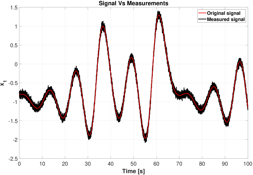
Figure 1. Original signal overlaid onto the noisy signal created by adding measurement noise generated as filtered Gaussian noise in the band 0-200 Hz.

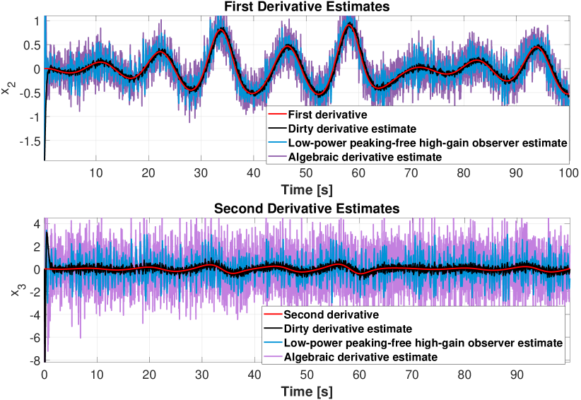
Figure 2. Comparison between estimates for the first and second derivatives of the signal in Figure 1 provided by the dirty derivative method, the peaking-free low-power high-gain observer and the algebraic derivative method.

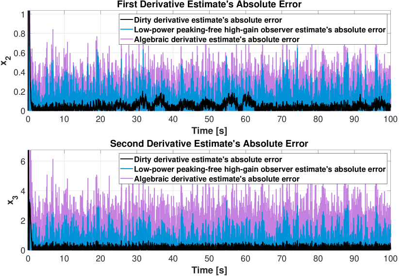
Figure 3. Comparison between absolute estimation error for the first and second derivatives of the signal in Figure 1 provided by the dirty derivative method, the peaking-free low-power high-gain observer and the algebraic derivative method.

These figures underscore the potential robustness against measurement noise that dirty derivatives can offer. The next subsection emphasizes this point in a closed-loop example.

6.2. Dirty-derivatives in closed-loop

In this subsection we provide simulation examples for the results presented in Section 4. Starting with the former, we consider system (3.1) with:

$$A_{n}=\begin{bmatrix}-1&3&3&0&1\end{bmatrix},\ B_{n}=-4,\ x_{0}=\begin{bmatrix}-1&5&-1&-3&3\end{bmatrix}.$$

A large number of simulations were performed where each of the entries of the above entities were chosen randomly as integers in the interval $[-5,5]$ with uniform probability. Consistent performance was evidenced through these simulations and the above set of values was chosen as a good representation of the observed behavior.

We design the linear controller $u=Kx$ where $K$ is obtained by solving the linear quadratic regulator problem with costs $Q=C^{T}C$ and $R=0.001$, and measurements satisfy the equation: $y=Cx+v,$ where $v$ is generated as in the previous section with a variance of $0.01$. We then implement $u=K\widehat{x}$ where $\widehat{x}$ is computed through: dirty derivatives as in (2.3) with $\sigma=75$; algebraic derivative estimation as in [KMB18] with $a=75$; and a high-gain observer as in section 2.2 in [Kha02] where the poles of $H_{0}$ are set at $\{-1,-2,-3,-4,-5\}$ and $\varepsilon=\frac{1}{75}$.

Figures 4 and 5 respectively compare the trajectories and absolute trajectory tracking errors for these three close-loop systems. Note that all three methods achieve similar steady state performance despite the varying levels of complexity in their implementations. Regarding the transient, we observe both the dirty-derivative and the algebraic estimation methods to be less affected by peaking than the high-gain observer.

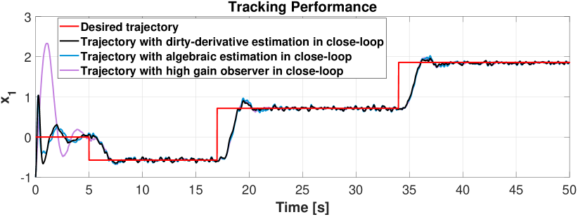
Figure 4. Comparison between the desired trajectory and the achieved trajectories by the controller $u=K\widehat{x}$ when estimates are provided by the dirty derivative method, a high-gain observer and the algebraic derivative method.

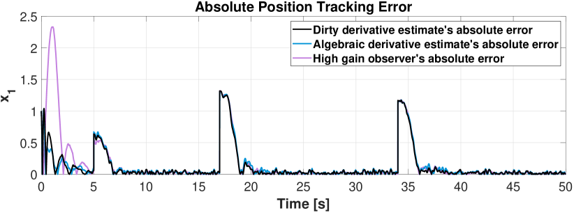
Figure 5. Comparison of absolute tracking error incurred by the controller $u=K\widehat{x}$ when estimates are provided by the dirty derivative method, a high-gain observer and the algebraic derivative method.

7. Conclusion

In this paper we have provided two Lyapunov based proofs enabling the use of dirty derivatives in place of observers when performing output feedback for a large class of linear time invariant systems, i.e., arbitrary order systems in canonical control form. Being independent of the plant’s model or inputs, having a single tuning parameter, low gains and noise attenuation characteristics, positions the dirty derivatives as an easy-to-use, straight forward estimation method. Future research involves their extension to general observable and controllable systems, along with investigating the relationships between dirty derivatives and the algebraic estimation method presented in [KMB18].

8. Appendix

8.1. Proof of Theorem (4.2)

Theorem 8.1.

There always exists $\underline{\sigma}\in{\mathbb{R}}_{>0}$ such that for any $\sigma\in(\underline{\sigma},\infty)$ the linear time invariant dynamical system (4.1) is asymptotically stable.

Proof.

We prove the above claim by a Lyapunov argument. First we introduce a set of $\frac{n(n+1)}{2}$ error variables that we index as:

(8.1) $$\forall i\in\{1,2,\dots,n\},\forall j \in\{0,1,\dots,n-i\}:$$

$$e_{i,j}=\widehat{x}_{i}^{(j)}-x_{i+j},$$

where the superscript in parenthesis denotes the $j$-th derivative of a variable with respect to time. Note that the maximum value of $j$ is $n-i$, so that $i+j\leq n$ and the error term $e_{i,j}$ is always well-defined.

To ease the exposition of our method, the newly defined error variables are organized in a matrix as follows, with the $i,j$-th entry denoting the error variable $e_{i,j-1}$:

(8.2) $$E =\begin{bmatrix}e_{1,0}&e_{1,1}&\dots&e_{1,n-1}\\ e_{2,0}&e_{2,1}&\dots&0\\ \vdots&\vdots&\iddots&\vdots\\ e_{n,0}&0&\dots&0\end{bmatrix}$$

$$=\begin{bmatrix}\widehat{x}_{1}-x_{1}&\dot{\widehat{x}}_{1}-x_{2}&\dots&\widehat{x}_{1}^{(n-2)}-x_{n}\\ \widehat{x}_{2}-x_{2}&\dot{\widehat{x}}_{2}-x_{3}&\dots&0\\ \vdots&\vdots&\iddots&\vdots\\ \widehat{x}_{n}-x_{n}&0&\dots&0\end{bmatrix}.$$

Given (8.1), the time derivatives of the error variables are given by:

(8.3) $$\dot{e}_{i,j}=\dot{\widehat{x}}_{i}^{(j)}-\dot{x}_{i+j} =-\sigma\left(\widehat{x}_{i}-\dot{\widehat{x}}_{i-1}\right)^{(j)}-\dot{x}_{i+j}$$

$$=-\sigma(\widehat{x}_{i}^{(j)}-\widehat{x}_{i-1}^{(j+1)})-\dot{x}_{i+j},$$

where the second equality is obtained by substituting $\dot{\widehat{x}}_{i}$ with the corresponding right-hand side in the equations of the dynamical system (4.1). Furthermore, note that we have defined $\dot{\widehat{x}}_{0}=x_{1}$ for conciseness. We now introduce a set of properties that these error derivatives possess that are instrumental in the rest of the proof:

1. If $i=1$:

   $$\widehat{x}_{i}^{(j)}-\widehat{x}_{i-1}^{(j+1)} =\widehat{x}_{1}^{(j)}-\widehat{x}_{0}^{(j+1)}=\widehat{x}_{1}^{(j)}-x_{1}^{(j)}$$

   $$=\widehat{x}_{1}^{(j)}-x_{1+j}=e_{1,j}.$$

2. If $i>1$:
   We notice from (8.1) that $e_{i-1,j+1}=\widehat{x}_{i-1}^{(j+1)}-x_{i+j}$. Then:

   $$\widehat{x}_{i}^{(j)}-\widehat{x}_{i-1}^{(j+1)} =\widehat{x}_{i}^{(j)}-e_{i-1,j+1}-x_{i+j}$$

   $$=e_{i,j}-e_{i-1,j+1}.$$

3. If $i+j<n$:

   $$\dot{x}_{i+j}=x_{i+j+1}.$$

4. If $i+j=n$:

   $$\dot{x}_{i+j} =A_{n}x+B_{n}K\begin{bmatrix}\widehat{x}_{1}&\widehat{x}_{2}&\dots&\widehat{x}_{n}\end{bmatrix}^{T}$$

   $$=A_{n}x$$

   $$\ +B_{n}K\begin{bmatrix}x_{1}+e_{1,0}&x_{2}+e_{2,0}&\dots&x_{n}+e_{n,0}\end{bmatrix}^{T}$$

   $$=A_{n}x+B_{n}Kx+B_{n}K\begin{bmatrix}e_{1,0}&e_{2,0}&\dots&e_{n,0}\end{bmatrix}^{T}$$

   $$=K^{*}x+B_{n}Ke_{0},$$

   where we define $e_{0}=\begin{bmatrix}e_{1,0}&e_{2,0}&\dots&e_{n,0}\end{bmatrix}^{T},$ and $K^{*}=A_{n}+B_{n}K.$

As a result of these properties, we compute and organize the error derivatives in a new matrix, as shown in (8.4) at the top of the next page.

(8.4) $$\dot{E}=\begin{bmatrix}-\sigma e_{1,0}-x_{2}&-\sigma e_{1,1}-x_{3}&\dots&-\sigma e_{1,n-1}-K^{*}x-B_{n}Ke_{0}\\ -\sigma e_{2,0}+\sigma e_{1,1}-x_{3}&-\sigma e_{2,1}+\sigma e_{1,2}-x_{4}&\dots&0\\ \vdots&\vdots&\iddots&\vdots\\ -\sigma e_{n,0}+\sigma e_{n-1,1}-K^{*}x-B_{n}Ke_{0}&0&\dots&0\end{bmatrix}$$

Moreover, using the error variables the time derivative of $x$ can be expressed as:

$$\dot{x} =Ax+BK\begin{bmatrix}\widehat{x}_{1}&\widehat{x}_{2}&\dots&\widehat{x}_{n}\end{bmatrix}^{T}$$

$$=Ax+BK\begin{bmatrix}x_{1}+e_{1,0}&x_{2}+e_{2,0}&\dots&x_{n}+e_{n,0}\end{bmatrix}^{T}$$

$$=(A+BK)x+BK\begin{bmatrix}e_{1,0}&e_{2,0}&\dots&e_{n,0}\end{bmatrix}^{T}$$

$$=(A+BK)x+BKe_{0}.$$

Let $e\in{\mathbb{R}}^{\frac{n(n+1)}{2}}$ denote the vector containing all the error variables $e_{i,j}$, and consider the following Lyapunov function $V:{\mathbb{R}}^{n}\times{\mathbb{R}}^{\frac{n(n+1)}{2}}\to{\mathbb{R}}_{\geq 0}$ of $x$ and $e$:

(8.5) $$V(x,e)=x^{T}Px+\sum_{i=1}^{n}\sum_{j=0}^{n-i}e_{i,j}^{2},$$

where $P$ is specified as defined in (3.3). We proceed to compute the time derivative of (8.5):

(8.6) $$\dot{V}= \dot{x}^{T}Px+x^{T}P\dot{x}+2\sum_{i=1}^{n}\sum_{j=0}^{n-i}e_{i,j}\dot{e}_{i,j}$$

$$= \left((A+BK)x+BKe_{0}\right)^{T}Px$$

$$+x^{T}P\left((A+BK)x+BKe_{0}\right)+2\sum_{i=1}^{n}\sum_{j=0}^{n-i}e_{i,j}\dot{e}_{i,j}$$

$$= -x^{T}Qx+2x^{T}PBKe_{0}-2K^{*}x\sum_{i=1}^{n}e_{i,n-i}$$

$$-2\sigma\left[\sum_{i=1}^{n}\sum_{j=0}^{n-i}e_{i,j}^{2}-\sum_{i=2}^{n}\sum_{j=0}^{n-i}e_{i,j}e_{i-1,j+1}\right]$$

$$-2B_{n}Ke_{0}\sum_{i=1}^{n}e_{i,n-i}-2\sum_{i=1}^{n-1}\sum_{j=0}^{n-i-1}e_{i,j}x_{i+j+1}.$$

The first term in the last equality was obtained through (3.3), and the last four terms were obtained by expanding $\sum_{i=1}^{n}\sum_{j=0}^{n-i}e_{i,j}\dot{e}_{i,j}$ according to (8.2) and (8.4).With the preceding at hand we can prove that (8.5) is strictly negative definite for sufficiently large values of $\sigma$. In the following we make repeated use of Lemma 8.2.

Lemma 8.2.

All triples ${a,b,\varepsilon}$ with $a,b\in{\mathbb{R}}^{n}$ and $\varepsilon\in{\mathbb{R}}_{>0}$ satisfy the inequality:

$$\pm 2a^{T}b\leq\varepsilon\lVert a\rVert^{2}+\frac{1}{\varepsilon}\lVert b\rVert^{2}.$$

We proceed by deriving upper bounds for all of the terms in (8.6).

1. Since $Q$ is strictly positive definite, we know that:

   $$-x^{T}Qx\leq-\lambda\lVert x\rVert^{2},$$

   where $\lambda$ is the smallest eigenvalue of $Q$.

2. By using Lemma (8.2) with $a=x$ and $b=PBKe_{0}$, we can write:

   $$2x^{T}PBKe_{0} \leq\varepsilon\lVert x\rVert^{2}+\frac{\lVert PBK\rVert^{2}}{\varepsilon}\lVert e_{0}\rVert^{2}$$

   $$\leq\varepsilon\lVert x\rVert^{2}+\frac{\lVert PBK\rVert^{2}}{\varepsilon}\sum_{i=1}^{n}\sum_{j=0}^{n-i}e_{i,j}^{2},$$

   for any $\varepsilon>0$.

3. By using Lemma (8.2) with $b=\sum_{i=1}^{n}e_{i,n-i}$ and $a=K^{*}x$, we can write:

   $$-2K^{*}x\sum_{i=1}^{n}e_{i,n-i} \leq\varepsilon\lVert K^{*}\rVert^{2}\lVert x\rVert^{2}+\frac{1}{\varepsilon}\left(\sum_{i=1}^{n}e_{i,n-i}\right)^{2}.$$

   Note that $\left(\sum_{i=1}^{n}e_{i,n-i}\right)^{2}$ is a strictly positive definite quadratic form, therefore there exists a constant $c_{1}\in{\mathbb{R}}_{>0}$ such that:

   $$\left(\sum_{i=1}^{n}e_{i,n-i}\right)^{2}\leq c_{1}\sum_{i=1}^{n}e_{i,n-i}^{2},$$

   allowing us to write:

   $$-2K^{*}x\sum_{i=1}^{n}e_{i,n-i} \leq\varepsilon\lVert K^{*}\rVert^{2}\lVert x\rVert^{2}+\frac{c_{1}}{\varepsilon}\sum_{i=1}^{n}e_{i,n-i}^{2}$$

   $$\leq\varepsilon\lVert K^{*}\rVert^{2}\lVert x\rVert^{2}+\frac{c_{1}}{\varepsilon}\sum_{i=1}^{n}\sum_{j=0}^{n-i}e_{i,j}^{2}.$$

4. Analogously to point 3, for some $c_{2}\in{\mathbb{R}}_{>0}$ and $\varepsilon=1$ we can write the bound:

   $$-2B_{n}Ke_{0} \sum_{i=1}^{n}e_{i,n-i}$$

   $$\leq\lVert B_{n}K\rVert^{2}\lVert e_{0}\rVert^{2}+\left(\sum_{i=1}^{n}e_{i,n-i}\right)^{2}$$

   $$\leq\lVert B_{n}K\rVert^{2}\sum_{i=1}^{n}\sum_{j=0}^{n-i}e_{i,j}^{2}+c_{2}\sum_{i=1}^{n}\sum_{j=0}^{n-i}e_{i,j}^{2}$$

   $$=\left(\lVert B_{n}K\rVert^{2}+c_{2}\right)\sum_{i=1}^{n}\sum_{j=0}^{n-i}e_{i,j}^{2}.$$

5. By repeatedly applying Lemma (8.2) with $a=x_{i+j+1}$ and $b=e_{i,j}$, we can write:

   $$-2\sum_{i=1}^{n-1} \sum_{j=0}^{n-i-1}e_{i,j}x_{i+j+1}$$

   $$\leq\sum_{i=1}^{n-1}\sum_{j=0}^{n-i-1}(\varepsilon x_{i+j+1}^{2}+\frac{1}{\varepsilon}e_{i,j}^{2})$$

   $$=\varepsilon\sum_{i=1}^{n-1}\sum_{j=0}^{n-i-1}x_{i+j+1}^{2}+\frac{1}{\varepsilon}\sum_{i=1}^{n-1}\sum_{j=0}^{n-i-1}e_{i,j}^{2},$$

   and again there exist constants $c_{3},c_{4}\in{\mathbb{R}}_{>0}$ allowing us to bound the above positive definite quadratic forms by:

   $$-2\sum_{i=1}^{n-1}\sum_{j=0}^{n-i-1}e_{i,j}x_{i+j+1}\leq\varepsilon c_{3}\lVert x\rVert^{2}+\frac{c_{4}}{\varepsilon}\sum_{i=1}^{n}\sum_{j=0}^{n-i}e_{i,j}^{2}.$$

6. The remaining term can be written as:

   $$-2\sigma\left[\sum_{i=1}^{n}\sum_{j=0}^{n-i}e_{i,j}^{2}-\sum_{i=2}^{n}\sum_{j=0}^{n-i}e_{i,j}e_{i-1,j+1}\right]$$

   $$\ =2\sigma\sum_{k=1}^{n}\left(-\sum_{\ell=0}^{k-1}e_{k-\ell,\ell}^{2}+\sum_{\ell=0}^{k-2}e_{k-\ell,\ell}e_{k-\ell-1,\ell+1}\right),$$

   where, through a slight abuse of notation, we define the sum $\sum\limits^{j}_{i}1$ to be zero whenever $j<i.$ Intuitively, the inner sums for specific values of $k$ correspond to summing the elements of $E\odot\dot{E}$ along its anti-diagonals including only the terms that are multiplied by $\sigma$, e.g., $k=1$ corresponds to the first anti-diagonal (the top left element), $k=2$ to the second anti-diagonal, etc.

   We claim that for any $k$ there exists a constant $d_{k}\in{\mathbb{R}}_{>0}$ such that:

   (8.7) $$-\sum_{\ell=0}^{k-1}e_{k-\ell,\ell}^{2}+\sum_{\ell=0}^{k-2}e_{k-\ell,\ell}e_{k-\ell-1,\ell+1}\leq-d_{k}\sum_{\ell=0}^{k-1}e_{k-\ell,\ell}^{2}.$$

   This can be shown by first defining $z_{\ell}=e_{k-\ell,\ell}$ and applying the following lemma.

   Lemma 8.3.

   For any $k\in{\mathbb{N}}_{>0}$, the quadratic form:

   $$-\sum_{i=1}^{k}z_{i}^{2}+\sum_{i=1}^{k-1}z_{i}z_{i+1}$$

   is negative definite.

   Finally, inequality (8.7) is reached by noting that the negative definiteness of the left terms implies the existence of $d_{k}\in{\mathbb{R}}_{>0}$ such that the inequality holds. Inequality (8.7) allows us to write:

   $$-2\sigma \left[\sum_{i=1}^{n}\sum_{j=0}^{n-i}e_{i,j}^{2}-\sum_{i=2}^{n}\sum_{j=0}^{n-i}e_{i,j}e_{i-1,j+1}\right]$$

   $$=2\sigma\sum_{k=1}^{n}\left(-\sum_{\ell=0}^{k-1}e_{k-\ell,\ell}^{2}+\sum_{\ell=0}^{k-2}e_{k-\ell,\ell}e_{k-\ell-1,\ell+1}\right)$$

   $$\leq-2\sigma\sum_{k=1}^{n}d_{k}\sum_{\ell=0}^{k-1}e_{k-\ell,\ell}^{2}\leq-2\sigma d\sum_{k=1}^{n}\sum_{\ell=0}^{k-1}e_{k-\ell,\ell}^{2}$$

   $$=-2\sigma d\sum_{i=1}^{n}\sum_{j=0}^{n-i}e_{i,j}^{2},$$

   where $\sum_{i=1}^{n}\sum_{j=0}^{n-i}e_{i,j}^{2}=\sum_{k=1}^{n}\sum_{\ell=0}^{k-1}e_{k-\ell,\ell}^{2},$ and $d=\min\{d_{1},d_{2},\dots,d_{n}\}.$

We can now provide the full upper bound for the time derivative of $V$:

$$\dot{V} \leq-x^{T}Qx+2x^{T}PBKe_{0}-2K^{*}x\sum_{i=1}^{n}e_{i,n-i}$$

$$\quad-2\sigma\left[\sum_{i=1}^{n}\sum_{j=0}^{n-i}e_{i,j}^{2}-\sum_{i=2}^{n}\sum_{j=0}^{n-i}e_{i,j}e_{i-1,j+1}\right]$$

$$\quad-2B_{n}Ke_{0}\sum_{i=1}^{n}e_{i,n-i}-2\sum_{i=1}^{n-1}\sum_{j=0}^{n-i-1}e_{i,j}x_{i+j+1}$$

$$\leq-\lambda\lVert x\rVert^{2}+\varepsilon\lVert x\rVert^{2}+\frac{\lVert PBK\rVert^{2}}{\varepsilon}\sum_{i=1}^{n}\sum_{j=0}^{n-1}e_{i,j}^{2}$$

$$\quad+\varepsilon\lVert K^{*}\rVert^{2}\lVert x\rVert^{2}+\frac{c_{1}}{\varepsilon}\sum_{i=1}^{n}\sum_{j=0}^{n-1}e_{i,j}^{2}$$

$$\quad+\left(\lVert B_{n}K\rVert^{2}+c_{2}\right)\sum_{i=1}^{n}\sum_{j=0}^{n-1}e_{i,j}^{2}+\varepsilon c_{3}\lVert x\rVert^{2}$$

$$\quad+\frac{c_{4}}{\varepsilon}\sum_{i=1}^{n}\sum_{j=0}^{n-1}e_{i,j}^{2}-2\sigma d\sum_{i=1}^{n}\sum_{j=0}^{n-1}e_{i,j}^{2}$$

$$\leq\left(-\lambda+\varepsilon\left(1+c_{3}+\lVert K^{*}\rVert^{2}\right)\right)\lVert x\rVert^{2}$$

$$\quad+\frac{1}{\varepsilon}\left(\lVert PBK\rVert^{2}+c_{1}+c_{4}\right)\sum_{i=1}^{n}\sum_{j=0}^{n-1}e_{i,j}^{2}$$

$$\quad+\left(\lVert B_{n}K\rVert^{2}+c_{2}-2\sigma d\right)\sum_{i=1}^{n}\sum_{j=0}^{n-1}e_{i,j}^{2}.$$

The above expression is negative definite as long as:

$$\varepsilon <\frac{\lambda}{1+c_{3}+\lVert K^{*}\rVert^{2}}$$

$$\sigma >\underline{\sigma}=\frac{\varepsilon^{-1}\left(\lVert PBK\rVert^{2}+c_{1}+c_{4}\right)+\lVert B_{n}K\rVert^{2}+c_{2}}{2d}.$$

We note that negative definiteness of $\dot{V}$ (in the state $x$ and the error variables $e$) implies $\lim_{t\to\infty}x=0$ and $\lim_{t\to\infty}e=0$. However, we know from (8.1) that the estimates $\widehat{x}_{1},\widehat{x}_{2},\dots,\widehat{x}_{n}$ can be represented as linear combinations of the state $x$ and the errors $e$, therefore we conclude that:

$$\forall i\in\{1,2,\dots,n\}:\quad\lim_{t\to\infty}\widehat{x}_{i}=0,$$

proving asymptotic stability for the original system (4.1). ∎

8.2. Proof of Theorem (5.1)

Theorem 8.4.

There always exists $\underline{\gamma}\in{\mathbb{R}}_{>0}$, such that for any $\gamma\in(\underline{\gamma},\infty)$ there exists $\underline{\sigma}\in{\mathbb{R}}_{>0}$ such that for any $\sigma\in(\underline{\sigma},\infty)$ the LTI dynamical system (5.3) is asymptotically stable.

Proof.

The proof proceeds largely analogously to the proof of Theorem 4.2. As before, we introduce the $\frac{n(n+1)}{2}$ error variables as defined in (8.1), that we can organize into matrix (8.2).

We define $e_{0}=\begin{bmatrix}e_{1,0}&e_{2,0}&\dots&e_{n-1,0}\end{bmatrix}^{T}$, and introduce a new error variable $e_{u}$, defined as:

(8.8) $$e_{u}=x_{n}-Kx_{1:n-1},$$

that allows us to rewrite $\dot{x}_{n}$ as:

$$\dot{x}_{n}= A_{n}\dot{x}_{1:n-1}-\beta\gamma\left(\widehat{x}_{n}-K\begin{bmatrix}\widehat{x}_{1}&\widehat{x}_{2}&\dots&\widehat{x}_{n-1}\end{bmatrix}^{T}\right)$$

$$= A_{n}\dot{x}_{1:n-1}-\beta\gamma(e_{u}+e_{n}-Ke_{0}),$$

and the derivatives of $x_{1},x_{2},\dots,x_{n-1}$ as:

$$\dot{x}_{1:n-1}=Ax_{1:n-1}+Bx_{n}=(A+BK)x_{1:n-1}+Be_{u},$$

where we used (8.8) to obtain the second equality.

As in (8.3), the time derivatives of the error variables are:

$$\dot{e}_{i,j} =-\sigma(\widehat{x}_{i}^{(j)}-\widehat{x}_{i-1}^{(j+1)})-\dot{x}_{i+j},$$

with the same properties as in Theorem 4.2, except for point 4 which now becomes:

1. If $i+j=n$:

   $$\dot{x}_{i+j}=\dot{x}_{n}=A_{n}\dot{x}_{1:n-1}-\beta\gamma e_{u}-\beta\gamma(e_{n}-Ke_{0}),$$

As a result, we again compute and organize the error derivatives in matrix form for clarity, as shown in (8.9) at the top of the next page.

(8.9) $$\dot{E}=\begin{bmatrix}-\sigma e_{1,0}-x_{2}&-\sigma e_{1,1}-x_{3}&\dots&-\sigma e_{1,n-1}+A_{n}\dot{x}_{1:n-1}-\beta\gamma(e_{u}e_{n}-Ke_{0})\\ -\sigma e_{2,0}+\sigma e_{1,1}-x_{3}&-\sigma e_{2,1}+\sigma e_{1,2}-x_{4}&\dots&0\\ \vdots&\vdots&\iddots&\vdots\\ -\sigma e_{n,0}+\sigma e_{n-1,1}+A_{n}\dot{x}_{1:n-1}-\beta\gamma(e_{u}+e_{n}-Ke_{0})&0&\dots&0\end{bmatrix}$$

Finally, we compute the derivative of $e_{u}$:

$$\dot{e}_{u}= \dot{x}_{n}-K\dot{x}_{1:n-1}$$

$$= -\beta\gamma\left(e_{u}+e_{n}-Ke_{0}\right)$$

$$-(K-A_{n})\left((A+BK)x_{1:n-1}+Be_{u}\right)$$

$$= -\beta\gamma\left(e_{u}+e_{n}-Ke_{0}\right)$$

$$-\overline{K}\left((A+BK)x_{1:n-1}+Be_{u}\right),$$

where we define $\overline{K}=K-A_{n}.$ We now consider the following Lyapunov function $V:{\mathbb{R}}^{n-1}\times{\mathbb{R}}\times{\mathbb{R}}^{\frac{n(n+1)}{2}}\to{\mathbb{R}}_{\geq 0}$ of $x$ and all the error variables, denoting the vector containing all the errors except $e_{u}$ by $e\in{\mathbb{R}}^{\frac{n(n+1)}{2}}$:

(8.10) $$V(x,e_{u},e)=x_{1:n-1}^{T}Px_{1:n-1}+e_{u}^{2}+\sum_{i=1}^{n}\sum_{j=0}^{n-i}e_{i,j}^{2}.$$

Computing the time derivative of (8.10) results in:

(8.11) $$\dot{V} =2x_{1:n-1}^{T}P\dot{x}_{1:n-1}+2e_{u}\dot{e}_{u}+2\sum_{i=1}^{n}\sum_{j=0}^{n-i}e_{i,j}\dot{e}_{i,j}$$

$$=-x_{1:n-1}^{T}Qx_{1:n-1}+2x_{1:n-1}^{T}PBe_{u}+2(-\beta\gamma-\overline{K}B)e_{u}^{2}$$

$$-2e_{u}\beta\gamma(e_{n}-Ke_{0})-2e_{u}\overline{K}(A+BK)x_{1:n-1}$$

$$-2\sigma\left[\sum_{i=1}^{n}\sum_{j=0}^{n-i}e_{i,j}^{2}-\sum_{i=2}^{n}\sum_{j=0}^{n-i}e_{i,j}e_{i-1,j+1}\right]$$

$$-2\beta\gamma e_{u}\sum_{i=1}^{n}e_{i,n-i}-2\beta\gamma(e_{n}-Ke_{0})\sum_{i=1}^{n}e_{i,n-i}$$

$$-2A_{n}(A+BK)x_{1:n-1}\sum_{i=1}^{n}e_{i,n-i}-2A_{n}Be_{u}\sum_{i=1}^{n}e_{i,n-i}$$

$$-2\sum_{i=1}^{n-1}\sum_{j=0}^{n-i-1}e_{i,j}x_{i+j+1}.$$

Just like in Theorem 4.2, we proceed by deriving upper bounds for all of the terms in (8.11). We make use of Lemma (8.2) every time we encounter a mixed product of variables.

1. Denoting the smallest eigenvalue of $Q$ by $\lambda$:

   $$-x_{1:n-1}^{T}Qx_{1:n-1}\leq-\lambda\lVert x_{1:n-1}\rVert^{2}.$$

2. For any $\varepsilon\in{\mathbb{R}}_{>0}$:

   $$2x_{1:n-1}^{T}PBe_{u}\leq\varepsilon\lVert x_{1:n-1}\rVert^{2}+\frac{\lVert PB\rVert^{2}}{\varepsilon}e_{u}^{2}.$$

3. For some constant $c_{1}\in{\mathbb{R}}_{>0}$:

   $$-2e_{u}\beta\gamma(e_{n}-Ke_{0}) \leq e_{u}^{2}+\beta^{2}\gamma^{2}(e_{n}-Ke_{0})^{2}$$

   $$\leq e_{u}^{2}+\beta^{2}\gamma^{2}c_{1}\sum_{i=1}^{n}\sum_{j=0}^{n-1}e_{i,j}^{2}.$$

4. For any $\varepsilon\in{\mathbb{R}}_{>0}$:

   $$-2e_{u}\overline{K}(A+BK) x_{1:n-1}\leq$$

   $$\varepsilon\lVert x_{1:n-1}\rVert^{2}+\frac{\lVert\overline{K}(A+BK)\rVert^{2}}{\varepsilon}e_{u}^{2}.$$

5. For some constant $c_{2}\in{\mathbb{R}}_{>0}$:

   $$-2\beta\gamma e_{u}\sum_{i=1}^{n}e_{i,n-i} \leq e_{u}^{2}+\beta^{2}\gamma^{2}\left(\sum_{i=1}^{n}e_{i,n-i}\right)^{2}$$

   $$\leq e_{u}^{2}+\beta^{2}\gamma^{2}c_{2}\sum_{i=1}^{n}\sum_{j=0}^{n-1}e_{i,j}^{2}.$$

6. For some constant $c_{3}\in{\mathbb{R}}_{>0}$:

   $$-2\beta\gamma(e_{n}-Ke_{0})\sum_{i=1}^{n}e_{i,n-i}\leq\beta\gamma c_{3}\sum_{i=1}^{n}\sum_{j=0}^{n-1}e_{i,j}^{2}.$$

7. For some $c_{4}\in{\mathbb{R}}_{>0}$ and any $\varepsilon\in{\mathbb{R}}_{>0}$:

   $$-2 A_{n}(A+BK)x_{1:n-1}\sum_{i=1}^{n}e_{i,n-i}$$

   $$\leq 2\lVert A_{n}(A+BK)\rVert\lVert x_{1:n-1}\rVert\lVert\sum_{i=1}^{n}e_{i,n-i}\rVert$$

   $$\leq\varepsilon\lVert x_{1:n-1}\rVert^{2}+\frac{\lVert A_{n}(A+BK)\rVert^{2}}{\varepsilon}\left(\sum_{i=1}^{n}e_{i,n-i}\right)^{2}$$

   $$\leq\varepsilon\lVert x_{1:n-1}\rVert^{2}+\frac{c_{4}}{\varepsilon}\sum_{i=1}^{n}\sum_{j=0}^{n-1}e_{i,j}^{2}$$

8. For some constant $c_{5}\in{\mathbb{R}}_{>0}$:

   $$-2A_{n}Be_{u}\sum_{i=1}^{n}e_{i,n-i} \leq e_{u}^{2}+(A_{n}B)^{2}\left(\sum_{i=1}^{n}e_{i,n-i}\right)^{2}$$

   $$\leq e_{u}^{2}+(A_{n}B)^{2}c_{5}\sum_{i=1}^{n}\sum_{j=0}^{n-1}e_{i,j}^{2}.$$

9. For some $c_{6},c_{7}\in{\mathbb{R}}_{>0}$ and any $\varepsilon\in{\mathbb{R}}_{>0}$:

   $$-2 \sum_{i=1}^{n-1}\sum_{j=0}^{n-i-1}e_{i,j}x_{i+j+1}$$

   $$= -2\sum_{i=1}^{n-1}\sum_{j=0}^{n-i-2}e_{i,j}x_{i+j+1}-2x_{n}\sum_{i=1}^{n-1}e_{i,n-i-1}$$

   $$= -2\sum_{i=1}^{n-1}\sum_{j=0}^{n-i-2}e_{i,j}x_{i+j+1}$$

   $$-2(e_{n}+Kx_{1:n-1})\sum_{i=1}^{n-1}e_{i,n-i-1}$$

   $$\leq \varepsilon c_{6}\lVert x_{1:n-1}\rVert^{2}+\frac{c_{7}}{\varepsilon}\sum_{i=1}^{n}\sum_{j=0}^{n-i}e_{i,j}^{2}.$$

   Note that all $x$ terms in the right-hand side of the second equality have indices between $1$ and $n-1$.

10. Exactly as in Theorem (4.2), for some $d\in{\mathbb{R}}_{>0}$:

    $$-2\sigma \left[\sum_{i=1}^{n}\sum_{j=0}^{n-i}e_{i,j}^{2}-\sum_{i=2}^{n}\sum_{j=0}^{n-i}e_{i,j}e_{i-1,j+1}\right]$$

    $$\leq-2\sigma d\sum_{i=1}^{n}\sum_{j=0}^{n-1}e_{i,j}^{2}.$$

Substituting all of these bounds in (8.11), we can bound $\dot{V}$ by:

$$\dot{V}\leq \left(-\lambda+\varepsilon(3+c_{6})\right)\lVert x_{1:n-1}\rVert^{2}$$

$$+\left(\frac{\lVert PB\rVert^{2}\lVert\overline{K}(A+BK)\rVert^{2}}{\varepsilon}-2\beta\gamma-2\overline{K}B+3\right)e_{u}^{2}$$

$$+\left(\beta^{2}\gamma^{2}(c_{1}+c_{2})+\beta\gamma c_{3}+\frac{c_{4}+c_{7}}{\varepsilon}\right)\sum_{i=1}^{n}\sum_{j=0}^{n-1}e_{i,j}^{2}$$

$$+\left((A_{n}B)^{2}c_{5}-2\sigma d\right)\sum_{i=1}^{n}\sum_{j=0}^{n-1}e_{i,j}^{2}.$$

The previous expression is negative definite as long as:

$$\varepsilon <\frac{\lambda}{3+c_{6}},$$

$$\gamma >\underline{\gamma}=\frac{1}{2\beta}\left(\frac{\lVert PB\rVert^{2}\lVert\overline{K}(A+BK)\rVert^{2}}{\varepsilon}-2\overline{K}B+3\right),$$

$$\sigma >\underline{\sigma}$$

$$=\frac{1}{2d}\left(\beta^{2}\gamma^{2}(c_{1}+c_{2})+\beta\gamma c_{3}+\frac{c_{4}+c_{7}}{\varepsilon}+(A_{n}B)^{2}c_{5}\right).$$

To finish the proof, we note that negative definiteness of $\dot{V}$ (in the state $x$ and the error variables $e$ (except $e_{u}$)) implies $\lim_{t\to\infty}x_{1:n-1}=0$, $\lim_{t\to\infty}e_{u}=0$ and $\lim_{t\to\infty}e=0$. However, both $x_{n}$ and the estimates $\widehat{x}_{1},\widehat{x}_{2},\dots,\widehat{x}_{n}$ are linear combinations of the state $x_{1:n-1}$, $e_{u}$, and the errors $e$, therefore we conclude that:

$$\forall i\in\{1,2,\dots,n\}:\quad\lim_{t\to\infty}\widehat{x}_{i}=0\ \text{and}\ \lim_{t\to\infty}x_{n}=0,$$

proving asymptotic stability for the original system (5.3). ∎

References

• [ACL05] Kiam Heong Ang, G. Chong, and Yun Li. Pid control system analysis, design, and technology. IEEE Transactions on Control Systems Technology, 13(4):559–576, 2005.
• [AH95] Karl Johan Aström and Tore Hägglund. PID Controllers: Theory, Design, and Tuning. ISA - The Instrumentation, Systems and Automation Society, 1995.
• [AH01] Karl Johan Aström and Tore Hägglund. The future of pid control. Control Engineering Practice, 9(11):1163–1175, 2001. PID Control.
• [Cha11] Rick Chartrand. Numerical differentiation of noisy, nonsmooth data. International Scholarly Research Notices, 2011, 2011.
• [DAT18] Laurent Praly Daniele Astolfi, Lorenzo Marconi and Andrew R. Teel. Low-power peaking-free high-gain observers. Automatica, 98:169–179, 2018.
• [EHN96] Heinz Werner Engl, Martin Hanke, and Andreas Neubauer. Regularization of inverse problems, volume 375. Springer Science & Business Media, 1996.
• [FFO17] Igor Furtat, Alexander Fradkov, and Yury Orlov. State feedback finite time sliding mode stabilization using dirty differentiation. IFAC-PapersOnLine, 50(1):9619–9624, 2017. 20th IFAC World Congress.
• [FMT21] Lucas Fraile, Matteo Marchi, and Paulo Tabuada. Data-driven stabilization of siso feedback linearizable systems, 2021.
• [JS18] Rayana H. Jaafar and Samer S. Saab. Sliding mode control with dirty derivatives filter for rigid robot manipulators. In 2018 9th IEEE Annual Ubiquitous Computing, Electronics Mobile Communication Conference (UEMCON), pages 716–720, 2018.
• [Kha02] Hassan K. Khalil. Nonlinear Systems. Pearson Education. Prentice Hall, 2002.
• [KMB18] Josip Kasac, Dubravko Majetic, and Danko Brezak. An algebraic approach to on-line signal denoising and derivatives estimation. Journal of the Franklin Institute, 355(15):7799–7825, 2018.
• [Lor16] Antonio Loria. Observers are unnecessary for output-feedback control of lagrangian systems. IEEE Transactions on Automatic Control, 61(4):905–920, 2016.
• [LP13] Shuai Lu and Sergei V Pereverzev. Regularization theory for ill-posed problems. de Gruyter, 2013.
• [MC20] Roger Miranda-Colorado. Parameter identification of conservative hamiltonian systems using first integrals. Applied Mathematics and Computation, 369:124860, 2020.
• [NH10] Eduardo Nunes and Liu Hsu. Global tracking for robot manipulators using a simple causal pd controller plus feedforward. Robotica, 28:23–34, 01 2010.
• [OWN+97] Alan V Oppenheim, Alan S Willsky, Syed Hamid Nawab, Gloria Mata Hernández, et al. Signals & systems. Pearson Educación, 1997.
• [SRZBH19] Hebertt Sira-Ramirez, Eric Zurita-Bustamante, and Congzhi Huang. Equivalence among flat filters, dirty derivative-based pid controllers, adrc, and integral reconstructor-based sliding mode control. IEEE Transactions on Control Systems Technology, PP:1–15, 06 2019.
• [VK06] Luma K. Vasiljevic and Hassan K. Khalil. Differentiation with high-gain observers the presence of measurement noise. In Proceedings of the 45th IEEE Conference on Decision and Control, pages 4717–4722, 2006.