Pivot Gray Codes for the Spanning Trees of a Graph ft. the Fan

Abstract

We consider the problem of listing all spanning trees of a graph $G$ such that successive trees differ by pivoting a single edge around a vertex. Such a listing is called a “pivot Gray code”, and it has more stringent conditions than known “revolving-door” Gray codes for spanning trees. Most revolving-door algorithms employ a standard edge-deletion/edge-contraction recursive approach which we demonstrate presents natural challenges when requiring the “pivot” property. Our main result is the discovery of a greedy strategy to list the spanning trees of the fan graph in a pivot Gray code order. It is the first greedy algorithm for exhaustively generating spanning trees using such a minimal change operation. The resulting listing is then studied to find a recursive algorithm that produces the same listing in $O(1)$-amortized time using $O(n)$ space. Additionally, we present $O(n)$-time algorithms for ranking and unranking the spanning trees for our listing; an improvement over the generic $O(n^{3})$-time algorithm for ranking and unranking spanning trees of an arbitrary graph. Finally, we discuss how our listing can be applied to find a pivot Gray code for the wheel graph.

1 Introduction

Applications of efficiently listing all spanning trees of general graphs are ubiquitous in computer science and also appear in many other scientific disciplines [4]. In fact, one of the earliest known works on listing all spanning trees of a graph is due to the German physicist Wilhelm Feussner in 1902 who was motivated by an application to electrical networks [8]. In the 120 years since Feussner’s work, many new algorithms have been developed, such as those in the following citations [1, 5, 7, 9, 10, 13, 14, 15, 17, 19, 20, 22, 23, 24, 25, 27].

For any application, it is desirable for spanning tree listing algorithms to have the asymptotically best possible running time, that is, $O(1)$-amortized running time. The algorithms due to Kapoor and Ramesh [15], Matsui [19], Smith [25], Shioura and Tamura [23] and Shioura et al. [24] all run in $O(1)$-amortized time. Another desirable property of such listings is to have the revolving-door property, where successive spanning trees differ by the addition of one edge and the removal of another. Such listings where successive objects in a listing differ by a constant number of simple operations are more generally known as Gray codes. The algorithms due to Smith [25], Kamae [14], Kishi and Kajitani [17], Holzmann and Harary [13] and Cummins [7] all produce Gray code listings of spanning trees for an arbitrary graph. Of all of these algorithms, Smith’s is the only one that produces a Gray code listing in $O(1)$-amortized time.

Example 1  Consider the fan graph on five vertices illustrated in Figure 1, where the seven edges are labeled

$$e_{1}=v_{1}v_{2},\ e_{2}=v_{1}v_{\infty},\ e_{3}=v_{2}v_{3},\ e_{4}=v_{2}v_{\infty},\ e_{5}=v_{3}v_{4},\ e_{6}=v_{3}v_{\infty},\ e_{7}=v_{4}v_{\infty}.$$

The following is a revolving-door Gray code for the 21 spanning trees of this graph. The initial spanning tree has edges $\{e_{1},e_{2},e_{5},e_{6}\}$ and each step of the listing below provides the edge that is removed from the current tree followed by the new edge that is added to obtain the next tree in the listing:

1. $-e_{5}+e_{7}$	8. $-e_{5}+e_{7}$	15. $\bm{-e_{7}+e_{3}}$
2. $-e_{1}+e_{3}$	9. $-e_{4}+e_{3}$	16. $-e_{2}+e_{4}$
3. $-e_{3}+e_{4}$	10. $-e_{6}+e_{5}$	17. $-e_{1}+e_{2}$
4. $-e_{7}+e_{5}$	11. $\bm{-e_{5}+e_{2}}$	18. $-e_{4}+e_{7}$
5. $-e_{4}+e_{3}$	12. $-e_{2}+e_{4}$	19. $-e_{3}+e_{4}$
6. $-e_{2}+e_{1}$	13. $-e_{3}+e_{5}$	20. $-e_{5}+e_{3}$.
7. $-e_{3}+e_{4}$	14. $-e_{4}+e_{2}$

This listing was generated from Knuth’s implementation of Smith’s [25] algorithm provided at http://combos.org/span. The steps in red are highlighted to show where the edge moves do not pivot around a vertex.

A stronger notion of a Gray code for spanning trees is where the revolving-door makes strictly local changes. More specifically, we would like the edges being removed and added at each step to share a common endpoint. We call a listing with this property a pivot Gray code (also known as a strong revolving-door Gray code [18]). The aforementioned spanning tree Gray codes are not pivot Gray codes. In particular, the Gray code given by Smith’s algorithm [25] is not a pivot Gray code as illustrated in our previous example: the highlighted edge moves 11 and 15 do not have the “pivot” property. This leads to our first research question.

Research Question #1  Given a graph $G$ (perhaps from a specific class), does there exist a pivot Gray code listing of all spanning trees of $G$? Furthermore, can the listing be generated in polynomial time per tree using polynomial space?

A short discussion as to why previous methods do not lead directly to pivot Gray codes is presented in Section 1.3.

A related question that arises for any listing is how to rank, that is, find the position of the object in the listing, and unrank, that is, return the object at a specific rank. For spanning trees, an $O(n^{3})$-time algorithm for ranking and unranking a spanning tree of a specific listing for an arbitrary graph is known [6].

Research Question #2  Given a graph $G$ (perhaps from a specific class), does there exist a (pivot Gray code) listing of all spanning trees of $G$ that can be ranked and unranked in $O(n^{2})$ time or better?

An algorithmic technique recently found to have success in the discovery of Gray codes is the greedy approach. An algorithm is said to be greedy if it can prioritize allowable actions according to some criteria, and then choose the highest priority action that results in a unique object to obtain the next object in the listing. When applying a greedy algorithm, there is no backtracking; once none of the valid actions lead to a new object in the set under consideration, the algorithm halts, even if the listing is not exhaustive. The work by Williams [26] notes that some very well-known combinatorial listings can be constructed greedily, including the binary reflected Gray code (BRGC) for binary strings, the plain change order for permutations, and the lexicographically smallest de Bruijn sequence. Recently, a very powerful greedy algorithm on permutations (known as Algorithm J, where J stands for “jump”) generalizes many known combinatorial Gray code listings including many related to permutation patterns, rectangulations, and elimination trees [11, 12, 21]. However, no greedy algorithm was previously known to list the spanning trees of an arbitrary graph.

Research Question #3  Given a graph $G$ (perhaps from a specific class), does there exist a greedy strategy to list all spanning trees of $G$? Moreover, is the resulting listing a pivot Gray code?

In most cases, a greedy algorithm requires exponential space to recall which objects have already been visited in a listing. Thus, answering this third question would satisfy only the first part of Research Question #1. However, in many cases, an underlying pattern can be found in a greedy listing which can result in space efficient algorithms [11, 26]. In recent communication with Arturo Merino, a greedy algorithm for listing the spanning trees of an arbitrary graph $G$ has been discovered by considering each tree’s characteristic vector and transposing elements to change the shortest possible prefix; however, it does not yield a pivot Gray code.

To address these three research questions, we applied a variety of greedy approaches to structured classes of graphs including the fan, wheel, $n$-cube, and the compete graph. From this study, we were able to affirmatively answer each of the research questions for the fan graph. It remains an open question to find similar results for other classes of graphs.

1.1 New results

The fan graph on $n$ vertices, denoted $F_{n}$, is obtained by joining a single vertex (which we label $v_{\infty}$) to the path on $n-1$ vertices (labeled $v_{2},...,v_{n}$) – see Figure 1. Note that we label

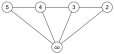
Figure 1: The fan $F_{5}$

the smallest vertex $v_{2}$ so that the largest non-infinity labeled vertex equals the total number of vertices. We discover a greedy strategy to generate the spanning trees of $F_{n}$ in a pivot Gray code order. We describe this greedy strategy in Section 2. The resulting listing is studied to find an $O(1)$-amortized time recursive algorithm that produces the same listing using only $O(n)$ space, which is presented in Section 3. We also show how to rank and unrank a spanning tree of the greedy listing in $O(n)$ time in Section 3, which is a significant improvement over the general $O(n^{3})$-time ranking and unranking that is already known. The proofs for our main technical results are in Section 4. We conclude with a summary in Section 5, along with a discussion as to how our pivot Gray code for the fan can be extended to the wheel.

A complete C implementation of our algorithms is available in the Appendix. A preliminary version of this paper appeared in COCOON 2021 [3].

1.2 Oriented spanning trees

Although we only consider undirected graphs in this paper, we point out a related open problem for directed graphs.

Given a directed graph $D$ and a fixed root vertex $r$, an oriented spanning tree or spanning arborescence is an oriented subtree $T$ of $D$ with $n-1$ arcs such that there is a unique path from $r$ to every other vertex in $D$; all the arcs are directed away from $r$ in $T$. The problem of finding a revolving-door Gray code for oriented spanning trees remains an open problem with a difficulty rating of 46/50 as given by Knuth in problem 102 on page 481 of [18]. Knuth also notes on page 804 that a solution to this problem for a fixed root $r$ implies that a strong revolving-door (pivot) Gray code exists for the spanning trees of an undirected graph. The mapping here is natural: given an undirected graph $G$, replace all edges $(u,v)$ with two directed edges, one from $u$ to $v$ and one from $v$ to $u$. Algorithms to list all oriented spanning trees with a given root are known [9, 16]; however, neither have the revolving-door property.

1.3 Edge contraction and deletion

A technique applied in the construction of several “revolving-door” Gray codes [22, 25, 27] is to recursively partition the spanning trees of a graph $G$ into those containing a specific edge $e$ by applying edge contraction, and those that do not contain the edge $e$ by deleting $e$. However, when applying this strategy to construct a pivot Gray code, there are challenges when it comes to uncontracting an edge. Specifically, even if we have a pivot Gray code for the spanning trees in $G/e$ ($G$ with the edge $e$ contracted), once we uncontract $e$, it does not necessarily result in a pivot Gray code for the original graph $G$. See, for example Figure 2.

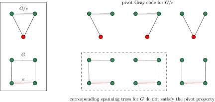
Figure 2: Illustrating how a pivot Gray code in graph $G/e$ does not necessarily correspond to a pivot Gray code for the spanning trees of $G$ that include $e$.

2 A greedy approach

Every unicyclic graph has a cyclic pivot Gray code: start with any initial spanning tree then pivot the edges around the cycle one at time. Thus, when considering greedy approaches for discovering a pivot Gray code we focused on the next obvious graph classes: the complete graph $K_{n}$, the fan $F_{n}$, the wheel $W_{n}$, and the $n$-cube. There are two important issues when considering a greedy approach to list spanning trees: (1) the labels on the vertices (or edges) and (2) the starting tree. For each of our approaches, we prioritized our operations by first considering which vertex $u$ to pivot on, followed by an ordering of the endpoints considered in the addition/removal. We call the vertex $u$ the pivot.

Our initial attempts focused only on pivots that were leaves. As a specific example, we ordered the leaves (pivots) from smallest to largest. Since each leaf $u$ is attached to a unique vertex $v$ in the current spanning tree, we then considered the neighbours of $u$ in increasing order of label. We restricted the labeling of the vertices to the most natural ones, such as the one presented in Section 1.1 for the fan. For each strategy we tried all possible starting trees. Unfortunately, none of our attempts lead to exhaustive listings for $K_{n}$, $F_{n}$, $W_{n}$, or the $n$-cube.

By allowing the pivot to be any arbitrary vertex, we ultimately discovered several exhaustive listing for the spanning trees of $F_{n}$; however, rather interestingly, we found no such listing for any other class. The listings we found for the fan were generated up to $n=12$. Starting from every starting tree for $n=12$ took about 8 hours on a single processor. One listing stood out as having an easily defined starting tree as well as a nice pattern which we could study to construct the listing more efficiently. It applied the labeling of the vertices as described in Section 1.1 with the following prioritization of pivots and their incident edges:

Prioritize the pivots $u$ from smallest to largest and then for each pivot, prioritize the edges $uv$ that can be removed from the current tree in increasing order of the label on $v$, and for each such $v$, prioritize the edges $uw$ that can be added to the current tree in increasing order of the label on $w$.

Since this is a greedy strategy, if an edge pivot results in a spanning tree that has already been generated or a graph that is not a spanning tree, then the next highest priority edge pivot is attempted. Let Greedy$(T)$ denote the listing that results from applying this greedy approach starting with the spanning tree $T$. The starting tree that produced a nice exhaustive listing was the path $v_{\infty},v_{2},v_{3},\ldots,v_{n}$, denoted $P_{n}$ throughout the paper. Figure 3 shows the listings Greedy$(P_{n})$ for $n=2,3,4,5$. The listing Greedy$(P_{6})$ is illustrated in Figure 4. It is worth noting that starting with the path $v_{\infty},v_{n},v_{n-1},\ldots,v_{2}$ or the star (all edges incident to $v_{\infty}$) did not lead to an exhaustive listing for the spanning trees of $F_{n}$ in our study.

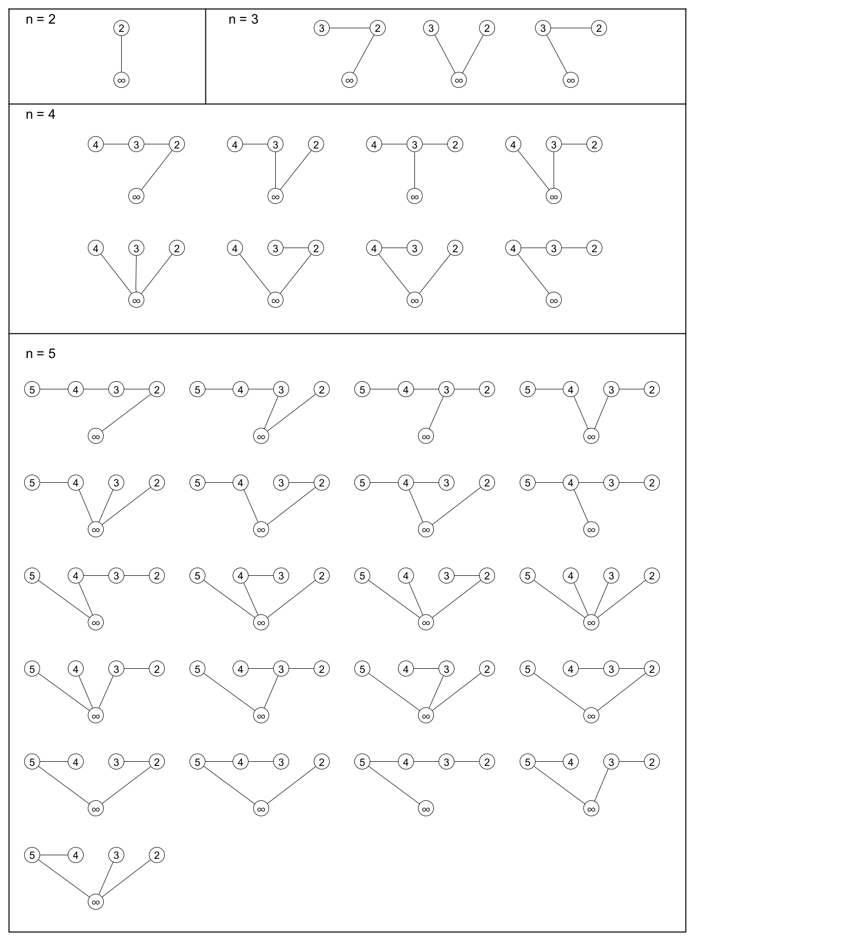
Figure 3: Greedy$(P_{n})$ for $n=2,3,4,5$. Read left to right, top to bottom.

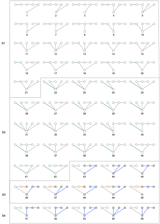
Figure 4: Greedy$(P_{6})$ read from left to right, top to bottom. Observe that S1 is Greedy$(P_{5})$ with $v_{6}v_{5}$ added, S2 is the reverse of Greedy$(P_{5})$ with $v_{6}v_{\infty}$ added, S3 is Greedy$(P_{4})$ with $v_{6}v_{5}$ and $v_{6}v_{\infty}$ added, except the edge $v_{4}v_{\infty}$ is replaced by $v_{4}v_{5}$, and S4 is the last five trees of Greedy$(P_{4})$ in reverse order ($v_{4}v_{\infty}$ is now present) with $v_{6}v_{5}$ and $v_{6}v_{\infty}$ added.

Example 2  Consider the listing Greedy$(P_{5})$ in Figure 3. When the current tree $T$ is the 16th one in the listing (the one with edges $\{v_{2}v_{\infty},v_{2}v_{3},v_{3}v_{4},v_{5}v_{\infty}\}$), the first pivot considered is $v_{2}$. Since both $v_{2}v_{3}$ and $v_{2}v_{\infty}$ are present in the tree, no valid move is available by pivoting on $v_{2}$. The next pivot considered is $v_{3}$. Both edges $v_{3}v_{2}$ and $v_{3}v_{4}$ are incident with $v_{3}$. First, we attempt to remove $v_{3}v_{2}$ and add $v_{3}v_{\infty}$, which results in a tree previously generated. Next, we attempt to remove $v_{3}v_{4}$ and add $v_{3}v_{\infty}$, which results in a cycle. So, the next pivot, $v_{4}$, is considered. The only edge incident to $v_{4}$ is $v_{4}v_{3}$. By removing $v_{4}v_{3}$ and adding $v_{4}v_{5}$ we obtain a new spanning tree, the next tree in the greedy listing.

To prove that Greedy$(P_{n})$ does in fact contain all the spanning trees of $F_{n}$, the next section demonstrates it is equivalent to a recursively constructed listing obtained by studying the greedy listings. Before we describe this recursive construction we mention one rather remarkable property of Greedy$(P_{n})$ that we prove later in Section 4.

Remark 2.1.

Let $X_{n}$ be last tree in the listing Greedy$(P_{n})$. Then Greedy$(X_{n})$ is precisely Greedy$(P_{n})$ in reverse order.

3 A pivot Gray code for the spanning trees of $F_{n}$ via recursion

In this section we develop an efficient recursive algorithm to construct the listing Greedy$(P_{n})$. The construction generates some sub-lists in reverse order, similar to the recursive construction of the BRGC. The recursive properties allow us to provide efficient ranking and unranking algorithms for the listing based on counting the number of trees at each stage of the construction. Let $t_{n}$ denote the number of spanning trees of $F_{n}$. It is known that

$$t_{n}=f_{2(n-1)}=2\frac{((3-\sqrt{5})/2)^{n}-((3+\sqrt{5})/2)^{n-2}}{5-3\sqrt{5}},$$

where $f_{n}$ is the $n$th number of the Fibonacci sequence with $f_{1}=f_{2}=1$ [2].

3.1 Pivot Gray code construction

By studying the order of the spanning trees in Greedy$(P_{n})$, we identified four distinct stages S1, S2, S3, S4 that are highlighted for Greedy$(P_{6})$ in Figure 4. From this figure, and referring back to Figure 3 to see the recursive properties, observe that:

• The trees in S1 are equivalent to Greedy$(P_{5})$ with the added edge $v_{6}v_{5}$.

• The trees in S2 are equivalent to the reversal of the trees in Greedy$(P_{5})$ with the added edge $v_{6}v_{\infty}$.

The trees in S3 and S4 have both edges $v_{6}v_{5}$ and $v_{6}v_{\infty}$ present.

• In S3, focusing only on the vertices $v_{4},v_{3},v_{2},v_{\infty}$, the induced subgraphs correspond to Greedy$(P_{4})$, except whenever $v_{4}v_{\infty}$ is present, it is replaced with $v_{4}v_{5}$ (the last five trees).

• In S4, focusing only on the vertices $v_{4},v_{3},v_{2},v_{\infty}$, the induced subgraphs correspond to the trees in Greedy$(P_{4})$ where $v_{4}v_{\infty}$ is present, in reverse order.

Generalizing these observations for all $n\geq 2$ leads to the recursive procedure given in Algorithm 1, called Gen($k,s_{1},\mathit{varEdge}$). It uses a global variable $T$ to store the current spanning tree with $n$ vertices. The parameter $k$ indicates the number of vertices under consideration; the parameter $s_{1}$ indicates whether or not to generate the trees in stage S1, as required by the trees for S4; and the parameter $\mathit{varEdge}$ indicates whether or not a variable edge needs to be added as required by the trees for S3. The base cases correspond to the edge moves in the listings Greedy$(P_{2})$ and Greedy$(P_{3})$.

Let $\mathcal{G}_{n}$ denote the listing obtained by initializing $T$ to $P_{n}$, printing $T$, and calling Gen($n,1,0$).

Algorithm 1

1:procedure Gen($k,s_{1},varEdge$)

2:    if $k=2$ then $\triangleright$ $F_{2}$ base case

3:        if $varEdge$ then $T\leftarrow T-v_{2}v_{\infty}+v_{2}v_{3}$; Print$(T)$         

4:    else if $k=3$ then $\triangleright$ $F_{3}$ base case

5:        if $s_{1}$ then

6:           if $varEdge$ then $T\leftarrow T-v_{3}v_{2}+v_{3}v_{4}$; Print$(T)$

7:           else $T\leftarrow T-v_{3}v_{2}+v_{3}v_{\infty}$; Print$(T)$                    

8:        $T\leftarrow T-v_{2}v_{\infty}+v_{2}v_{3}$; Print$(T)$

9:    else

10:        if $s_{1}$ then

11:           Gen$(k-1,1,0)$ $\triangleright$ S1

12:           if $varEdge$ then $T\leftarrow T-v_{k}v_{k-1}+v_{k}v_{k+1}$; Print$(T)$

13:           else $T\leftarrow T-v_{k}v_{k-1}+v_{k}v_{\infty}$; Print$(T)$                    

14:        RevGen$(k-1,1,0)$ $\triangleright$ S2

15:        $T\leftarrow T-v_{k-1}v_{k-2}+v_{k-1}v_{k}$; Print$(T)$

16:        Gen$(k-2,1,1)$ $\triangleright$ S3

17:        if $k>4$ then $T\leftarrow T-v_{k-2}v_{k-1}+v_{k-2}v_{\infty}$; Print$(T)$         

18:        RevGen$(k-2,0,0)$ $\triangleright$ S4     

Before discussing RevGen, we first provide a formal description of the last tree in the listing $\mathcal{G}_{n}$, which we denote $L_{n}$. Define the tree $Last_{n}$ as follows for $n\geq 2$: for $n=2,3,4$ let $Last_{n}$ be the last trees in the listings for $n=2,3,4$ given in Figure 3, and for $n>4$ let

$$Last_{n}=Last_{n-3}+v_{n}v_{n-1}+v_{n}v_{\infty}+v_{n-2}v_{\infty}.$$

Applying this definition, the trees $Last_{n}$ for $2\leq n\leq 7$ are given in Figure 5. The following lemma is proved in Section 4.

Lemma 3.1.

For $n\geq 2$, $L_{n}=Last_{n}$.

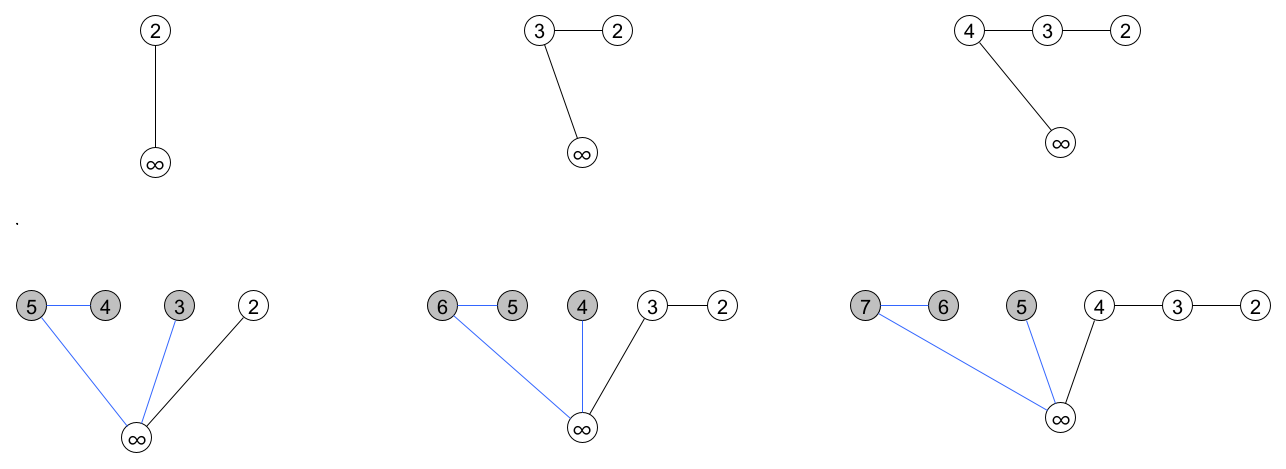
Figure 5: From left to right. {$Last_{2}$, $Last_{3}$, $Last_{4}$} (top), {$Last_{5}$, $Last_{6}$, $Last_{7}$} (bottom). Shaded vertices and blue edges highlight the additional vertices and edges added to the trees in the top row to obtain the trees in the bottom row.

The procedure RevGen($k,s_{1},\mathit{varEdge}$), performs the operations of Gen($k,s_{1},\mathit{varEdge}$) in reverse order, thus producing the reversal of the listing generated by Gen($k,s_{1},\mathit{varEdge}$) when starting with the last tree from the latter listing. The base cases correspond to the edge moves in the reversals of the listings Greedy$(P_{2})$ and Greedy$(P_{3})$.

Let $\mathcal{R}_{n}$ denote the listing obtained by initializing $T$ to $L_{n}$, printing $T$, and calling RevGen($n,1,0$).

Remark 3.2.

$\mathcal{R}_{n}$ is the listing $\mathcal{G}_{n}$ in reverse order.

Algorithm 2

1:procedure RevGen($k,s_{1},varEdge$)

2:    if $k=2$ then $\triangleright$ $F_{2}$ base case

3:        if $varEdge$ then $T\leftarrow T-v_{2}v_{3}+v_{2}v_{\infty}$; Print$(T)$         

4:    else if $k=3$ then $\triangleright$ $F_{3}$ base case

5:        $T\leftarrow T-v_{2}v_{3}+v_{2}v_{\infty}$; Print$(T)$

6:        if $s_{1}$ then

7:           if $varEdge$ then $T\leftarrow T-v_{3}v_{4}+v_{3}v_{2}$; Print$(T)$

8:           else $T\leftarrow T-v_{3}v_{\infty}+v_{3}v_{2}$; Print$(T)$                    

9:    else

10:        Gen$(k-2,0,0)$ $\triangleright$ S4

11:        if $k>4$ then $T\leftarrow T-v_{k-2}v_{\infty}+v_{k-2}v_{k-1}$; Print$(T)$         

12:        RevGen$(k-2,1,1)$ $\triangleright$ S3

13:        $T\leftarrow T-v_{k-1}v_{k}+v_{k-1}v_{k-2}$; Print$(T)$

14:        Gen$(k-1,1,0)$ $\triangleright$ S2

15:        if $s_{1}$ then

16:           if $varEdge$ then $T\leftarrow T-v_{k}v_{k+1}+v_{k}v_{k-1}$; Print$(T)$

17:           else $T\leftarrow T-v_{k}v_{\infty}+v_{k}v_{k-1}$; Print$(T)$            

18:           RevGen$(k-1,1,0)$ $\triangleright$ S1             

Theorem 3.3.

For $n\geq 2$, $\mathcal{G}_{n}$ and $\mathcal{R}_{n}$ are pivot Gray codes for the spanning trees of the fan $F_{n}$ and they can be generated in $O(1)$-amortized time using $O(n)$ space. Moreover, Greedy$(P_{n})$ = $\mathcal{G}_{n}$ and Greedy$(L_{n})$ = $\mathcal{R}_{n}$.

We prove this theorem in Section 4.

3.2 Ranking

Given a spanning tree $T$ in $\mathcal{G}_{n}$, we calculate its rank by recursively determining which stage (recursive call) $T$ is generated. We can determine the stage by focusing on the presence/absence of the edges $v_{n}v_{n-1}$, $v_{n}v_{\infty}$, $v_{n-2}v_{\infty}$, and $v_{n-2}v_{n-1}$. Based on the discussion of the recursive algorithm, there are $t_{n-1}$ trees generated in S1, $t_{n-1}$ trees generated in S2, $t_{n-2}$ trees generated in S3, and $t_{n-2}-t_{n-3}$ trees generated in S4. S3 is partitioned into two cases based on whether $v_{n-2}v_{n-1}$ ($varEdge)$ is present. For the remainder of this section we will let $T_{n-1}=T-v_{n}$ and $T_{n-2}=T-v_{n}-v_{n-1}$.

If $v_{n}v_{n-1},v_{n}v_{\infty},v_{n-2}v_{\infty}\in T$, then $T$ is a tree in S4 of $\mathcal{G}_{n}$. The trees of S4 are the trees of $\mathcal{G}_{n-2}$ without S1, listed in reverse order. So, the rank can be calculated by subtracting the rank of $T_{n-2}$ in $\mathcal{G}_{n-2}$ from $2t_{n-1}+2t_{n-2}$ (the rank of the last tree of S3 plus $t_{n-2}$). Note that we do not use $2t_{n-1}+2t_{n-2}-t_{n-3}$ because the recursive rank calculated already takes into account the trees of $S1$ that are missing.

If $v_{n}v_{n-1},v_{n}v_{\infty}\in T$ and $v_{n-2}v_{\infty}\not\in T$, then $T$ is a tree in S3 of $\mathcal{G}_{n}$. The trees of S3 are the trees of $\mathcal{G}_{n-2}$ where $v_{n-2}v_{\infty}$ has been replaced by $v_{n-2}v_{n-1}$. So, if $v_{n-2}v_{n-1}\in T$, then in order to recursively calculate the rank of $T_{n-2}$ in $\mathcal{G}_{n-2}$, we need to replace $v_{n-2}v_{n-1}$ with $v_{n-2}v_{\infty}$. If $v_{n-2}v_{n-1}\not\in T$, then no edge replacements are needed. We can then determine the rank of $T$ in $\mathcal{G}_{n}$ by adding the rank of $T_{n-2}$ in $\mathcal{G}_{n-2}$ to $2t_{n-1}$ (the rank of the last tree of S2).

The other two cases are fairly trivial. If $v_{n}v_{n-1}\in T$ and $v_{n}v_{\infty}\not\in T$, then $T$ is in S1. Since S1 is the trees of $\mathcal{G}_{n-1}$ with $v_{n}v_{n-1}$ added, we simply return the ranking of $T_{n-1}$ in $\mathcal{G}_{n-1}$. If $v_{n}v_{\infty}\in T$ and $v_{n}v_{n-1}\not\in T$, then $T$ is in S2. Since S2 is the trees of $\mathcal{G}_{n-1}$ in reverse order with $v_{n}v_{\infty}$ added, we return $2t_{n-1}+1$ (the rank of the first tree of S3) minus the rank of $T_{n-1}$ in $\mathcal{G}_{n-1}$.

For $n>1$, let $R_{n}(T)$ denote the rank of $T$ in the listing $\mathcal{G}_{n}$. If $n=2,3,4$, then $R_{n}(T)$ can easily be derived from Figure 3. Based on the above discussion, for $n\geq 5$:

$$R_{n}(T)=\begin{cases}2t_{n-1}+2t_{n-2}-R_{n-2}(T_{n-2})+1&\text{if $e_{1},e_{2},e_{3}\in T$}\\ 2t_{n-1}+R_{n-2}(T_{n-2}+e_{3})&\text{if $e_{1},e_{2},e_{4}\in T$, $e_{3}\not\in T$}\\ 2t_{n-1}+R_{n-2}(T_{n-2})&\text{if $e_{1},e_{2}\in T$, $e_{3},e_{4}\not\in T$}\\ 2t_{n-1}-R_{n-1}(T_{n-1})+1&\text{if $e_{2}\in T$, $e_{1}\not\in T$}\\ R_{n-1}(T_{n-1})&\text{if $e_{1}\in T$, $e_{2}\not\in T$}\end{cases}$$ (1)

where $e_{1}=v_{n}v_{n-1}$, $e_{2}=v_{n}v_{\infty}$, $e_{3}=v_{n-2}v_{\infty}$, and $e_{4}=v_{n-2}v_{n-1}$.

Example 3  Consider the spanning trees $T_{7}$, $T_{6}$, $T_{5}$, and $T_{3}$ for $F_{7},F_{6},F_{5}$ and $F_{3}$ respectively.

Observe that $T_{6}=T_{7}-v_{7}$, $T_{5}=T_{6}-v_{6}$, and $T_{3}=T_{5}-v_{5}-v_{4}+v_{3}v_{\infty}$. Consider $R_{7}(T)$ where $T=T_{7}$. Applying the formula in (1) we have

$$\begin{split}R_{7}(T)&=R_{6}(T_{6})\\ &=2t_{5}-R_{5}(T_{5})+1\\ &=43-(2t_{4}+R_{3}(T_{3}+v_{3}v_{\infty}))\\ &=43-(16+3)\\ &=24.\end{split}$$

Since each application of (1) requires constant time, and the recursion goes $O(n)$ levels deep, we arrive at the following result provided the first $2(n{-}2)$ Fibonacci numbers are precomputed. We note that the calculations are on numbers up to size $t_{n-1}$.

Theorem 3.4.

The listing $\mathcal{G}_{n}$ can be ranked in $O(n)$ time using $O(n)$ space under the unit cost RAM model.

3.3 Unranking

Determining the tree $T$ at rank $r$ in the listing $\mathcal{G}_{n}$ follows similar ideas by constructing $T$ starting from a set of $n$ isolated vertices and adding one edge at a time. If $0<r\leq t_{n-1}$ then $T$ must be a tree in S1 of $\mathcal{G}_{n}$. So, we can add $v_{n}v_{n-1}$ to $T$ and consider the rank $r$ tree in $\mathcal{G}_{n-1}$. If $t_{n-1}<r\leq 2t_{n-1}$, then $T$ is a tree in S2 of $\mathcal{G}_{n}$. Since $S2$ of $\mathcal{G}_{n}$ is simply $\mathcal{R}_{n-1}+v_{n}v_{\infty}$, we can add $v_{n}v_{\infty}$ to $T$ and then consider the rank $2t_{n-1}+1-r$ (rank of the first tree of S3 minus $r$) tree in $\mathcal{G}_{n-1}$. If $2t_{n-1}<r\leq 2t_{n-1}+t_{n-2}$, then $T$ must be a tree in S3 of $\mathcal{G}_{n}$. Since all trees in S3 have the edges $v_{n}v_{n-1}$ and $v_{n}v_{\infty}$, we can add these edges to $T$. Then, we can consider the rank $r-2t_{n-1}$ ($r$ minus the rank of the last tree of S2) tree of $\mathcal{G}_{n-2}$. Also note that since $T$ is in S3, $v_{n-2}v_{n-1}$ will replace $v_{n-2}v_{\infty}$ for the trees of $\mathcal{G}_{n-2}$. Otherwise, if $r>2t_{n-1}+t_{n-2}$, then $T$ must be in S4 of $\mathcal{G}_{n-2}$. Similar to S3, we can add $v_{n}v_{n-1}$ and $v_{n}v_{\infty}$ to $T$ as all trees in S4 have these edges. Then, we consider the $2t_{n-1}+2t_{n-2}-r+1$ (rank of the last tree of S3 plus the rank of the last tree of $\mathcal{G}_{n-2}$ minus $r$) tree of $\mathcal{G}_{n-2}$.

Let $U_{n}(r,\mathit{replaceEdge})$ return the edges that form the tree $T$ at rank $r$ for the listing $\mathcal{G}_{n}$. The parameter $\mathit{replaceEdge}$ indicates whether or not the edge $v_{n}v_{n+1}$ should be added instead of $v_{n}v_{\infty}$. Initially, $r$ is the specified rank, and $\mathit{replaceEdge}=0$. In the base cases where $n=2,3,4$, then $T$ is derived from Figure 3. For these cases, if the edge $v_{n}v_{\infty}$ is present and $\mathit{replaceEdge}=1$, then it is replaced by the edge $v_{n}v_{n+1}$. Based on the above discussion, we arrive at the following recursive construction for $U_{n}(r,\mathit{replaceEdge})$.

$$U_{n}(r,\mathit{replaceEdge})=\begin{cases}U_{n-1}(r,0)+v_{n}v_{n-1}&\text{if $0<r\leq t_{n-1}$,}\\ U_{n-1}(2t_{n-1}{-}r{+}1,0)+e&\text{if $t_{n-1}<r\leq 2t_{n-1}$,}\\ U_{n-2}(r{-}2t_{n-1},1)+v_{n}v_{n-1}+e&\text{if $2t_{n-1}<r\leq 2t_{n-1}{+}t_{n-2}$,}\\ U_{n-2}(2t_{n-1}{+}2t_{n-2}{-}r+1,0)+v_{n}v_{n-1}+e&\text{otherwise,}\par\par\par\end{cases}$$ (2)

where $e=v_{n}v_{n+1}$ if $\mathit{replaceEdge}=1$ and $e=v_{n}v_{\infty}$ otherwise.

Example 4  To find the 24th tree $T$ in the listing $\mathcal{G}_{7}$, we consider $U_{7}(24,0)$. Repeated application of (2) yields the following

$$U_{7}(24,0) = U_{6}(24,0)+v_{7}v_{6}\ \ \ \ \ \mbox{{\color[rgb]{0,0,1}$\triangleright$ since $0<24\leq t_{6}$}}$$

$$= U_{5}(19,0)+v_{7}v_{6}+v_{6}v_{\infty}\ \ \ \ \ \mbox{{\color[rgb]{0,0,1}$\triangleright$ since $t_{5}<24\leq 2t_{5}$}}$$

$$= U_{3}(3,1)+v_{7}v_{6}+v_{6}v_{\infty}+v_{5}v_{4}+v_{5}v_{\infty}\ \ \ \ \ \mbox{{\color[rgb]{0,0,1}$\triangleright$ since $2t_{4}<19\leq 2t_{4}+t_{3}$}}$$

$$= v_{7}v_{6}+v_{6}v_{\infty}+v_{5}v_{4}+v_{5}v_{\infty}+v_{3}v_{3}+v_{3}v_{2}\ \ \ \mbox{}$$

Reaching a base case, the 3rd tree of $\mathcal{G}_{3}$ is $\{v_{3}v_{2},v_{3}v_{\infty}\}$. Since $\mathit{replaceEdge}=1$, the edge $v_{3}v_{\infty}$ is replaced with $v_{3}v_{4}$ and we end up with the spanning tree $T$ containing the edges from the last line of the equation. These four steps to construct $T$ are illustrated below.

Since each application of (2) requires constant time, and the recursion goes $O(n)$ levels deep, we arrive at the following result provided the first $2(n{-}2)$ Fibonacci numbers are precomputed. We note that the calculations are on numbers up to size $t_{n-1}$.

Theorem 3.5.

The listing $\mathcal{G}_{n}$ can be unranked in $O(n)$ time using $O(n)$ space under the unit cost RAM model.

4 Proof of technical results

4.1 Proof of Theorem 3.3

To prove Theorem 3.3, we start by proving that the number of trees generated by $\mathcal{G}_{n}$ is $t_{n}$. Then we show that $\mathcal{G}_{n}$ = Greedy($P_{n}$) and $\mathcal{R}_{n}$ = Greedy($L_{n}$). Combining these results with the fact that the trees generated by the greedy approaches are unique and successive trees differ by the “pivot” of a single edge, we have that $\mathcal{G}_{n}$ $\mathcal{R}_{n}$ are pivot Gray codes for the spanning trees of the fan graph $F_{n}$. Finally, we verify the running time of the recursive algorithm to generate $\mathcal{G}_{n}$.

Before proving these results, we introduce some notation. Let $T-v_{i}$ denote the tree obtained from $T$ by deleting the vertex $v_{i}$ along with all edges that have $v_{i}$ as an endpoint. Let $T+v_{i}v_{j}$ (resp. $T-v_{i}v_{j}$) denote the tree obtained from $T$ by adding (resp. deleting) the edge $v_{i}v_{j}$. For the remainder of this section, we will let $T_{n}$ denote the tree $T$ specified as a global variable for Gen and RevGen, and we let $T_{n-1}=T-v_{n}$ and $T_{n-2}=T-v_{n}-v_{n-1}$.

Lemma 4.1.

For $n\geq 2$, $|\mathcal{G}_{n}|=|\mathcal{R}_{n}|=t_{n}$.

Proof 4.2.

We first note that since Gen and RevGen are exact reversals of each other, Gen$(n,s_{1},varEdge)$ starting with $T=P_{n}$ and RevGen$(n,s_{1},varEdge)$ starting with $T=L_{n}$ produce the same number of trees. The proof now proceeds by induction on $n$. It is easy to verify the result holds for $n=2,3,4$. Now assume $n>4$, and that $|\mathcal{G}_{j}|=t_{j}$, for $2\leq j<n$. We consider the number of trees generated by each of the four stages of Gen$(n-1,1,0)$ when starting with $P_{n}$.

S1: Since $n>4$ and $s_{1}=1$, Gen$(n-1,1,0)$ is executed. Since $T_{n}=P_{n}$, we have that $T_{n-1}=P_{n-1}$. So, by our inductive hypothesis, $t_{n-1}$ trees are printed. By definition of $L_{n}$, $T_{n-1}=L_{n-1}$ after Gen$(n-1,1,0)$. It follows that $T_{n}=L_{n-1}+v_{n}v_{n-1}$. Line 12 removes $v_{n}v_{n-1}$ and adds $v_{n}v_{\infty}$. Since $v_{n}v_{n-1}\in T$ and $v_{n}v_{\infty}\not\in T$, this results in one more tree printed. At this point, $T_{n}=L_{n-1}+v_{n}v_{\infty}$.

S2: Next, line 14 executes RevGen$(n-1,1,0)$. We have that $T_{n-1}=L_{n-1}$. So, by the inductive hypothesis, $t_{n-1}$ trees are printed. We know that $T_{n-1}=P_{n-1}$ after RevGen$(n-1,1,0)$ starting with $T_{n-1}=L_{n-1}$, so it follows that $T_{n}=P_{n-1}+v_{n}v_{\infty}$. Line 15 removes $v_{n-2}v_{n-1}$ and adds $v_{n-1}v_{n}$. Since $v_{n-2}v_{n-1}\in T$ (because $v_{n-2}v_{n-1}\in P_{n-1}$) and $v_{n-1}v_{n}\not\in T$, this results in one more tree printed. At this point, $T_{n}=P_{n-2}+v_{n}v_{\infty}+v_{n-1}v_{n}$.

S3: Line 16 then executes Gen$(n-2,1,1)$ with $T_{n-2}=P_{n-2}$ since $T_{n}=P_{n-2}+v_{n}v_{\infty}+v_{n-1}v_{n}$. Note that the only difference between Gen$(n-2,1,1)$ and Gen$(n-2,1,0)$ is that $v_{j}v_{j+1}$ is added instead of $v_{j}v_{\infty}$ since $n-2>2$. Also, $v_{n-2}v_{(n-2)+1}\not\in T_{n}$ so it can be added. It follows that Gen$(n-2,1,1)$ and Gen$(n-2,1,0)$ will output the same number of trees starting with $T_{n-2}=P_{n-2}$. So, line 16 results in $t_{n-2}$ trees printed, again by the inductive hypothesis. After line 16 is executed, we have $T_{n-2}=L_{n-2}-v_{n-2}v_{\infty}+v_{n-2}v_{n-1}$ since $varEdge$ was equal to $1$. Line 17 removes $v_{n-2}v_{n-1}$ and adds $v_{n-2}v_{\infty}$. Since $v_{n-2}v_{n-1}\in T$ and $v_{n-2}v_{\infty}\not\in T$, this results in one more tree printed. At this point, $T_{n}=L_{n-2}+v_{n}v_{n-1}+v_{n}v_{\infty}$.

S4: By our inductive hypothesis, $|\mathcal{R}_{n-2}|=t_{n-2}$. However, $s_{1}=0$ for line 18 (RevGen$(n-2,0,0)$). So, for RevGen$(n-2,0,0)$, line 17 (one tree) and line 18 ($t_{n-3}$ trees) are not executed. This results in a total of $t_{n-2}-t_{n-3}$ trees being printed by line 18 of Gen$(n,1,0)$.

In total, $2t_{n-1}+2t_{n-2}-t_{n-3}$ trees are printed. By a straightforward Fibonacci identity which we leave to the reader, we have that $t_{n}=2t_{n-1}+2t_{n-2}-t_{n-3}$. Therefore, $|\mathcal{G}_{n}|=|\mathcal{R}_{n}|=t_{n}$.

To prove the next result, we first detail some required terminology. If $T$ is a spanning tree of $F_{n}$, then we say that the operation of deleting an edge $v_{i}v_{j}$ and adding an edge $v_{i}v_{k}$ is a valid edge move of $T$ if the result is a spanning tree that has not been generated yet. Conversely, if the result is not a spanning tree, or the result is a tree that has already been generated, then it is not a valid edge move of $T$. We say an edge $v_{i}v_{j}$ is smaller than edge $v_{i}v_{k}$ if $j<k$. An edge move $T_{n}-v_{i}v_{j}+v_{i}v_{k}$ is said to be smaller than another edge move $T_{n}-v_{x}v_{y}+v_{x}v_{z}$ if $i<x$, if $i=x$ and $j<y$, or if $i=x$, $j=y$, and $k<z$.

Lemma 4.3.

For $n\geq 2$, $\mathcal{G}_{n}=\textsc{Greedy}(P_{n})$ and $\mathcal{R}_{n}=\textsc{Greedy}(L_{n})$.

Proof 4.4.

By induction on $n$. It is straightforward to verify that the result holds for $n=2,3,4$ by iterating through the algorithms. Assume $n>4$, and that $\mathcal{G}_{j}=\textsc{Greedy}(P_{j})$ and $\mathcal{R}_{j}=\textsc{Greedy}(L_{j})$ for $2\leq j<n$. We begin by showing $\mathcal{G}_{n}=\textsc{Greedy}(P_{n})$, breaking the proof into each of the four stages of a call to Gen$(n-1,1,0)$ starting with $P_{n}$.

S1: Since $n>4$ and $s_{1}=1$, Gen$(n-1,1,0)$ is executed. By our inductive hypothesis, $\mathcal{G}_{n-1}=\textsc{Greedy}(P_{n-1})$. These must be the first trees for Greedy$(P_{n})$, as any edge move involving $v_{n}v_{n-1}$ or $v_{n}v_{\infty}$ is larger than any edge move made by Greedy$(P_{n-1})$. Since Greedy$(P_{n-1})$ halts, it must be that no edge move of $T_{n-1}$ is possible. So Greedy$(P_{n})$ must make the next smallest edge move, which is $T_{n}-v_{n}v_{n-1}+v_{n}v_{\infty}$. Since $T_{n}$ is a spanning tree, it follows that $T_{n}-v_{n}v_{n-1}+v_{n}v_{\infty}$ is also a spanning tree (and has not been generated yet), and therefore the edge move is valid. At this point, Gen$(n,1,0)$ also makes this edge move, by line 13.

S2: RevGen$(n-1,1,0)$ ($T_{n-1}=L_{n-1}$) is then executed. By our inductive hypothesis, $\mathcal{R}_{n}=\textsc{Greedy}(L_{n-1})$. Since Greedy$(L_{n-1})$ halts, it must be that no edge moves of $T_{n-1}$ are possible. At this point, $T_{n-1}=P_{n-1}$ because RevGen$(n-1,1,0)$ was executed. The smallest edge move now remaining is $T_{n}-v_{n-2}v_{n-1}+v_{n}v_{n-1}$. This results in $T_{n}=P_{n-2}+v_{n}v_{n-1}+v_{n}v_{\infty}$, which is a spanning tree that has not been generated. So, Greedy$(P_{n})$ must make this move. Gen$(n,1,0)$ also makes this move, by line 15. So, $\mathcal{G}_{n}$ must equal Greedy$(P_{n})$ up to the end of S2.

S3: Next, Gen$(n-2,1,1)$ starting with $T_{n-2}=P_{n-2}$ is executed. Since $varEdge=1$, $v_{n-2}v_{n-1}$ is added instead of $v_{n-2}v_{\infty}$. Greedy$(P_{n})$ also adds $v_{n-2}v_{n-1}$ instead of $v_{n-2}v_{\infty}$ since $v_{n-2}v_{n-1}$ is smaller than $v_{n-2}v_{\infty}$ and this edge move results in a tree not yet generated. Other than the difference in this one edge move, which occurs outside the scope of $T_{n-2}$, Gen$(n-2,1,0)$ and Gen$(n-2,1,1)$ (both starting with $T_{n-2}=P_{n-2}$) make the same edge moves. Since we also know that $\mathcal{G}_{n-2}=\textsc{Greedy}(P_{n-2})$ by the inductive hypothesis, it follows that $\mathcal{G}_{n}$ continues to equal Greedy$(P_{n})$ after line 16 of Gen$(n,1,0)$ is executed. We know that $T_{n-2}=L_{n-2}$ after Gen$(n-2,1,0)$. However, $T_{n-2}=L_{n-2}-v_{n-2}v_{\infty}+v_{n-2}v_{n-1}$ instead because Gen$(n-2,1,1)$ was executed ($varEdge=1$). It must be that no edge moves of $T_{n-2}$ are possible because Greedy$(P_{n-2})$ (and Gen$(n-2,1,1)$) halted. The smallest edge move now remaining is $T_{n}-v_{n-2}v_{n-1}+v_{n-2}v_{\infty}$. This results in $T_{n-2}=L_{n-2}$. Also, $T_{n}=T_{n-2}+v_{n}v_{n-1}+v_{n}v_{\infty}$ is a spanning tree since $T_{n-2}$ is a spanning tree of $F_{n-2}$. So Greedy$(P_{n})$ makes this move. Gen$(n,1,0)$ also makes this move, by line 17, and thus $\mathcal{G}_{n}=\textsc{Greedy}(P_{n})$ up to the end of S3.

S4: Finally, RevGen$(n-2,0,0)$ starting with $T_{n-2}=L_{n-2}$ is executed. By our inductive hypothesis, $\mathcal{R}_{n-2}=\textsc{Greedy}(L_{n-2})$. From lines 15-18 of Algorithm 2, it is clear that RevGen$(n-2,0,0)$ and RevGen$(n-2,1,0)$ make the same edge moves until RevGen$(n-2,0,0)$ finishes executing. So, by the inductive hypothesis, the listings produced by RevGen$(n-2,0,0)$ and Greedy$(L_{n-2})$ are the same until this point, which is where Gen$(n,1,0)$ finishes execution. By Lemma 4.1 we have that $|\mathcal{G}_{n}|=t_{n}$. Therefore, Greedy$(P_{n})$ has also produced this many trees, and each tree is unique. Thus, it must be that all $t_{n}$ trees of $F_{n}$ have been generated. Thus, Greedy$(P_{n})$ also halts.

Since $\mathcal{G}_{n}$ and Greedy$(P_{n})$ start with the same tree, produce the same trees in the same order, and halt at the same place, it follows that $\mathcal{G}_{n}=\textsc{Greedy}(P_{n})$. We now prove that $\mathcal{R}_{n}=\textsc{Greedy}(L_{n})$. By using our inductive hypothesis and the same arguments as previously, we see that this results hold within the four stages of RevGen$(n,1,0)$ when starting with $L_{n}$(namely, Gen$(T_{n-2},0,0)$, RevGen$(T_{n-2},1,1)$, Gen$(T_{n-1},1,0)$, and RevGen$(T_{n-1},1,0)$). However, we must still prove that $\mathcal{R}_{n}$ matches $\textsc{Greedy}(L_{n})$ as we move between stages.

After S4: After Gen$(n-2,0,0)$, $T_{n}=L_{n-2}+v_{n}v_{n-1}+v_{n}v_{\infty}$. Since $v_{n-2}v_{\infty}\in T_{n}$ and no edge moves of $T_{n-2}$ are possible (because Greedy$(L_{n-2})$ halted), Greedy makes the next smallest edge move which is $T_{n}-v_{n-2}v_{\infty}+v_{n-2}v_{n-1}$. RevGen$(n,1,0)$ also makes this move here, by line 11.

After S3: After RevGen$(n-2,1,1)$, $T_{n}=P_{n-2}+v_{n}v_{n-1}+v_{n}v_{\infty}$. No edge moves of $T_{n-2}$ are possible at this point. Therefore, since $v_{n}v_{n-1}\in T_{n}$ and $v_{n-2}v_{n-1}\not\in T_{n}$, Greedy makes the smallest possible edge move which is $T_{n}-v_{n}v_{n-1}+v_{n-2}v_{n-1}$. RevGen$(n,1,0)$ also makes this move here, by line 13.

After S2: Finally, after Gen$(n-1,1,0)$, $T_{n}=L_{n-1}+v_{n}v_{\infty}$. No edge moves of $T_{n-1}$ are possible at this point. Therefore, Greedy must make the only remaining edge move, which is $T_{n}-v_{n}v_{\infty}+v_{n}v_{n-1}$. RevGen$(n,1,0)$ also makes this move here, by line 17.

Since Greedy$(L_{n})$ and RevGen$(n,1,0)$ start with the same tree, produce the same trees in the same order, and halt at the same place, it follows that $\mathcal{R}_{n}=\textsc{Greedy}(L_{n})$.

Because Greedy$(P_{n})$ generates unique spanning trees of $F_{n}$, Lemma 4.1 together with Lemma 4.3 implies the following.

Lemma 4.5.

For $n\geq 2$, $\mathcal{G}_{n}$ = Greedy$(P_{n})$ is a pivot Gray code listing for the spanning trees of $F_{n}$.

It remains to prove how efficiently our pivot Gray codes can be generated. To store the global tree $T$, the algorithms Gen and RevGen can employ an adjacency list model where each edge $uv$ is associated only with the smallest labeled vertex $u$ or $v$. This means $v_{\infty}$ will never have any edges associated with it, and every other vertex will have at most 3 edges in its list. Thus the tree $T$ requires at most $O(n)$ space to store, and edge additions and deletions can be done in constant time. The next result completes the proof of Theorem 3.3.

Lemma 4.6.

For $n\geq 2$, $\mathcal{G}_{n}$ and $\mathcal{R}_{n}$ can be generated in $O(1)$-amortized time using $O(n)$ space.

Proof 4.7.

For each call to Gen$(n,s_{1},varEdge)$ where $n>3$, there are at most four recursive function calls, and at least two new spanning trees generated. Thus, the total number of recursive calls made is at most twice the number of spanning trees generated. Each edge addition and deletion can be done in constant time as noted earlier. Thus each recursive call requires a constant amount of work, and hence the overall algorithm will run in $O(1)$-amortized time. There is a constant amount of memory used at each recursive call and the recursive stack goes at most $n-3$ levels deep; this requires $O(n)$ space. As mentioned earlier, the global variable $T$ stored as adjacency lists also requires $O(n)$ space.

4.2 Proof of Lemma 3.1

We prove that $L_{n}=Last_{n}$ for $n\geq 2$ by induction on $n$ and tracing the routines Gen and RevGen. By definition of $Last_{n}$, the result holds for $n=2,3,4$. Assume that $L_{j}=Last_{j}$ for $2\leq j<n$. Recall that $L_{n}$ is the last tree generated by a call to Gen$(n,1,0)$ when starting with the tree $P_{n}$. Tracing this routine following the proof of Lemma 4.3, the current spanning tree when calling RevGen$(n-2,0,0)$ (on line 18) is $L_{n-2}+v_{n}v_{n-1}+v_{n}v_{\infty}$. Thus from the definition of $Last_{n}$, we must show that the last tree of RevGen$(n-2,0,0)$ when starting with $L_{n-2}$ is $Last_{n-3}+v_{n-2}v_{\infty}$.

Since RevGen$(k,1,0)$ starting with $L_{k}$ is the reversal of Gen$(k,1,0)$ starting with $P_{k}$, then the last tree of S2 of RevGen$(k,1,0)$ must be the first tree of S2 of Gen$(k,1,0)$. The last tree of the recursive call S1 of Gen$(k,1,0)$ when starting with $P_{k}$ is $Last_{k-1}+v_{k}v_{k-1}$ because, by the inductive hypothesis, $L_{k-1}=Last_{k-1}$, and $v_{k}v_{k-1}\in P_{k}$. Then, the edge move made by line 13 of Gen$(k,1,0)$ removes $v_{k}v_{k-1}$ and adds $v_{k}v_{\infty}$. It follows that the first tree of S2 of Gen$(k,1,0)$, and equivalently the last tree of S2 of RevGen$(k,1,0)$, which is also the last tree of RevGen$(k,0,0)$ when starting with $L_{k}$, is $Last_{k-1}+v_{k}v_{\infty}$. Thus, the last tree of RevGen$(n-2,0,0)$ starting with $L_{n-2}$ is $Last_{n-3}+v_{n-2}v_{\infty}$, as desired.

5 Conclusion

We answer each of the three Research Questions outlined in Section 1 in the affirmative for the fan graph, $F_{n}$. First, we discovered a greedy algorithm that exhaustively listed all spanning trees of $F_{n}$ experimentally for small $n$ with an easy to define starting tree. We then studied this listings which led to a recursive construction producing the same listing that runs in $O(1)$-amortized time using $O(n)$ space. We also proved that the greedy algorithm does in fact exhaustively list all spanning trees of $F_{n}$ for all $n\geq 2$, by demonstrating the listing is equivalent to the aforementioned recursive algorithm. It is the first greedy algorithm known to exhaustively list all spanning trees for a non-trivial class of graphs. Finally, we provided $O(n)$-time ranking and unranking algorithms for our listings, assuming the unit cost RAM model. It remains an interesting open problem to answer the research questions for other classes of graphs including the wheel, $n$-cube, and complete graph.

5.1 Final comment: The wheel

The wheel $W_{n}$ is obtained by adding the single edge $v_{2}v_{n}$ to $F_{n}$. With the addition of this single edge, we were unable to find a greedy algorithm to list all the spanning trees of $W_{n}$ in a pivot Gray code order. However, we were able to adapt the recursive algorithm for the spanning trees of $F_{n}$ to obtain a pivot Gray code for $W_{n}$ by appropriately inserting the spanning trees of $W_{n}$ that contain the wheel edge $v_{2}v_{n}$.

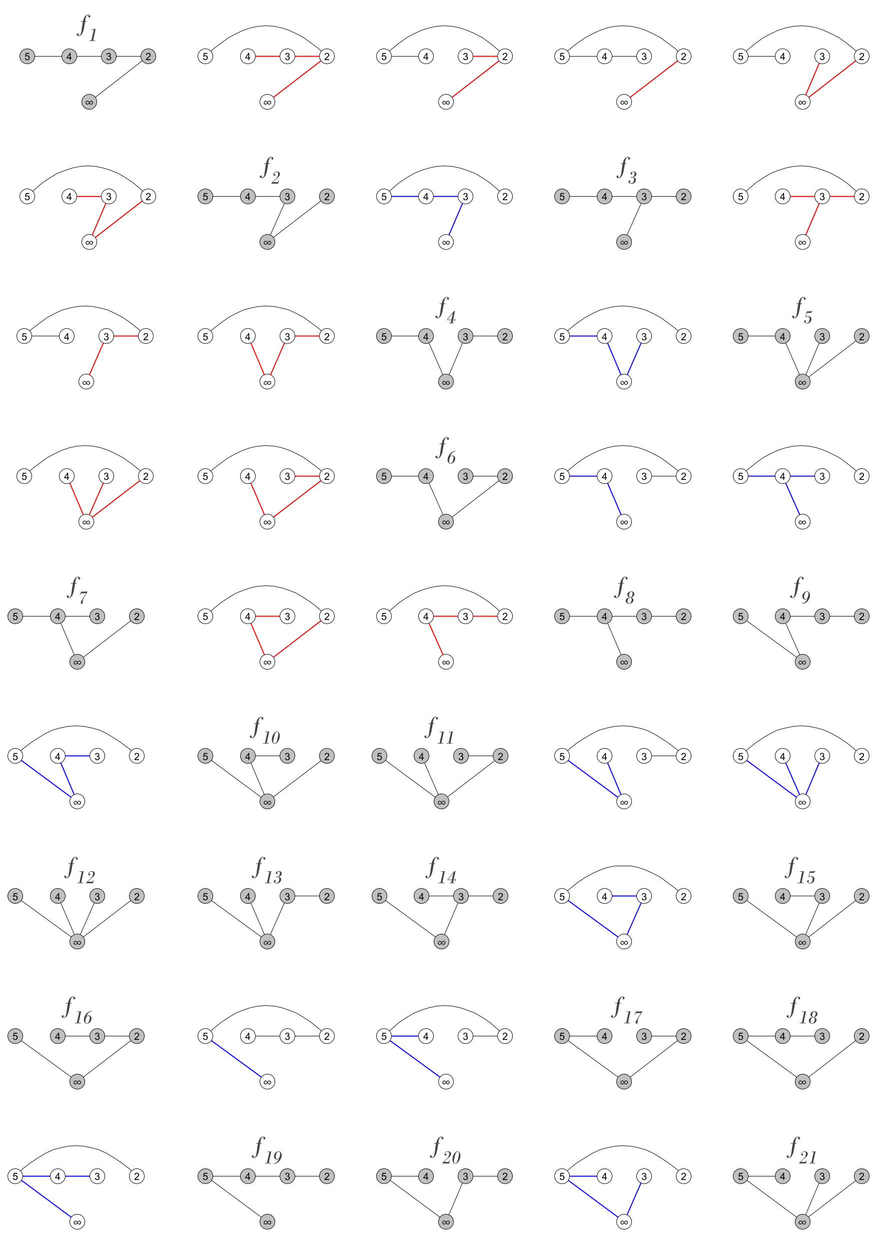
Figure 6: A pivot Gray code listing for the $W_{5}$ obtained by inserting the spanning trees with the edge $v_{2}v_{5}$ in between the trees of $\mathcal{G}_{5}$ (colored with grey vertices). The label $f_{j}$ denotes the $j$th tree of $\mathcal{G}_{5}$. Blue and red are used to highlight the edges of a left or right subgraph, respectively.

Figure 6 provides an example of a pivot Gray code listing for the spanning trees of $W_{5}$ obtained by inserting the trees containing the edge $v_{5}v_{2}$ into the listing for $\mathcal{G}_{5}$. Note that all the trees containing the wheel edge $v_{5}v_{2}$ contain subgraphs corresponding to the spanning trees of $F_{4}$, $F_{3}$, or $F_{2}$. For example, the second tree in the first row contains the first spanning tree of $\mathcal{G}_{4}$ as a subgraph (highlighted in red) on the vertices $v_{4},v_{3},v_{2},$ and $v_{\infty}$. The third tree of the second row also contains the first tree of $\mathcal{G}_{4}$, except this time it appears as a subgraph (highlighted in blue) on the vertices $v_{5},v_{4},v_{3},$ and $v_{\infty}$. We now introduce some terminology to differentiate between these two cases. A tree, $T$, with the wheel edge contains a right subgraph if $v_{2}$ is connected to $v_{\infty}$ when the edge $v_{n}v_{2}$ is removed from $T$. Similarly, $T$ contains a left subgraph if $v_{n}$ is connected to $v_{\infty}$ when the edge $v_{n}v_{2}$ is removed from $T$. As a further example of trees that contain right subgraphs, see the third and fourth tree on the first row, which contain the first tree of $\mathcal{G}_{3}$ and the first tree of $\mathcal{G}_{2}$, respectively.

When inserting the trees with the wheel edge, it is straightforward to fit in the trees that contain right subgraphs due to the recursive nature of Gen. Since the trees of S1 of Gen$(n,1,0)$ are all of the trees of Gen$(n-1,1,0)$ with the edge $v_{n}v_{n-1}$ added, we can add trees containing the wheel edge and these right subgraphs as intermediate trees in between the trees of S1 of $\mathcal{G}_{n}$ by removing the edge $v_{n}v_{n-1}$ and adding $v_{n}v_{2}$. We can further insert the trees containing smaller subgraphs (like the third and fourth tree on the first row) by rotating edges along the path, as seen in between $f_{1}$ and $f_{2}$ of Figure 6. Note that in between the fourth and fifth tree of the first row, we make the original edge move between $f_{1}$ and $f_{2}$, and then rotate edges back along the path to obtain $f_{2}$.

Unfortunately, the trees containing left subgraphs do not follow a nice recursive pattern. However, we are still able to insert them appropriately by considering two cases. First, when $v_{2}$ is the pivot vertex, we can insert a single tree containing a left subgraph as an intermediate edge move. As an example of this, see the tree in between $f_{2}$ and $f_{3}$ of Figure 6. The other case is when $v_{2}v_{\infty}$ is present and $v_{2}$ is not the pivot vertex, in which case we can insert two trees. For example, in between the trees labeled $f_{6}$ and $f_{7}$ in Figure 6. Note that we require $v_{2}v_{\infty}$ to be present so that we can remove it and add $v_{n}v_{2}$ as an intermediate move. If we instead replaced either $v_{2}v_{\infty}$ or $v_{2}v_{3}$ with $v_{n}v_{2}$, then we could end up with duplicate trees. Also note that generating right subgraphs takes precedence over generating left subgraphs. For example, even though our first case is satisfied in between $f_{7}$ and $f_{8}$, there are still trees with right subgraphs that can be generated, so we do not generate a tree with a left subgraph. Finally, note that inserting trees in the ways we have described does not change the relative order that the trees of $\mathcal{G}_{n}$ appear.

Appendix A C Code

⬇

#include <stdio.h>

#include <stdlib.h>

#define MAX_N 30

int n;

int tree[MAX_N+2][MAX_N+2]; // Adjacency matrix of a spanning tree

long long int fib[2*MAX_N+1]; // Stores the Fibonacci numbers

long long int numTrees = 1; // Number of trees generated

void ReverseGen(int k, int S1, int varEdge);

//-------------------------------------------------

void PrintMove(int v, int old, int new) {

printf("Move #%lld: -(%d, %d) +(%d, %d)\n", numTrees, v-1, old-1, v-1, new-1);

}

//-------------------------------------------------

void PrintTree() { // Prints edge list of tree

for (int i = 2; i < n+1; i++) {

for (int j = i+1; j < n+2; j++) {

if (tree[i][j] == 1) {

printf("%d %d\n", i-1, j-1);

}

}

} printf("\n");

}

//-------------------------------------------------

int tF(int k) { return fib[2*k - 2]; } // Calculates t(F_k)

//-------------------------------------------------

void CreateStartTree() { // Creates adjacency matrix of P_n

tree[2][n+1] = tree[n+1][2] = 1;

for (int i = 3; i < n+1; i++) {

tree[i][i-1] = tree[i-1][i] = 1;

}

}

//-------------------------------------------------

void CreateLastTree(int k) { // Creates adjacency matrix of L_n

if (k == 2) {

tree[2][n+1] = tree[n+1][2] = 1;

} else if (k == 3) {

tree[2][3] = tree[3][2] = 1;

tree[3][n+1] = tree[n+1][3] = 1;

} else if (k == 4) {

tree[2][3] = tree[3][2] = 1;

tree[3][4] = tree[4][3] = 1;

tree[4][n+1] = tree[n+1][4] = 1;

} else if (k > 4){

tree[k][k-1] = tree[k-1][k] = 1;

tree[k][n+1] = tree[n+1][k] = 1;

tree[k-2][n+1] = tree[n+1][k-2] = 1;

CreateLastTree(k-3);

}

}

//-------------------------------------------------

void CreateFib() { // Populates the Fibonacci array

fib[1] = fib[2] = 1;

for (int i = 3; i <= 2*(MAX_N-1); i++) fib[i] = fib[i-1] + fib[i-2];

}

//-------------------------------------------------

int Rank(int k) {

// Base cases

if (k == 3) { // F_3

if (tree[k][k-1] == 1 && tree[k][n+1] == 1) return 3;

else if (tree[k][n+1] == 1) return 2;

else if (tree[k][k-1] == 1) return 1;

}

else if (k == 2) { // F_2

if (tree[k][n+1] == 1) return 1;

}

if (tree[k][k-1] == 1 && tree[k][n+1] == 1) { // Both edges present

if (tree[k-2][n+1] == 1) return 2*tF(k-1) + 2*tF(k-2) - Rank(k-2) + 1*(k!=4); // S4

else if (tree[k-2][k-1] == 1) {

// Delete e_4, Add e_3 and continue as normal

tree[k-2][k-1] = tree[k-1][k-2] = 0;

tree[k-2][n+1] = tree[n+1][k-2] = 1;

}

return 2*tF(k-1) + Rank(k-2) + 1*(k==4); // S3

}

else if (tree[k][k-1] == 1) return Rank(k-1); // S1

else if (tree[k][n+1] == 1) return 2*tF(k-1) - Rank(k-1) + 1; // S2

return 0;

}

//-------------------------------------------------

void Unrank(int k, int rank, int replaceEdge) {

// Base cases

if (k == 2) { // F_2

if (replaceEdge == 1) tree[3][2] = tree[2][3] = 1;

else tree[n+1][2] = tree[2][n+1] = 1;

return;

}

else if (k == 3) { // F_3

if (rank == 1) {

tree[n+1][2] = tree[2][n+1] = 1; tree[2][3] = tree[3][2] = 1;

}

else if (rank == 2) {

tree[2][n+1] = tree[n+1][2] = 1;

if (replaceEdge == 1) tree[3][4] = tree[4][3] = 1;

else tree[n+1][3] = tree[3][n+1] = 1;

}

else if (rank == 3) {

tree[3][2] = tree[2][3] = 1;

if (replaceEdge == 1) tree[3][4] = tree[4][3] = 1;

else tree[3][n+1] = tree[n+1][3] = 1;

}

return;

}

if (rank <= tF(k-1)) { // S1 - Add e_1

tree[k][k-1] = tree[k-1][k] = 1;

Unrank(k-1, rank, 0);

}

else if (rank <= 2*tF(k-1)) { // S2 - Add e_2

if (replaceEdge == 1) tree[k][k+1] = tree[k+1][k] = 1;

else tree[k][n+1] = tree[n+1][k] = 1;

Unrank(k-1, 2*tF(k-1) - rank + 1, 0);

}

else if (rank <= 2*tF(k-1) + tF(k-2)) { // S3 - Add both edges

tree[k][k-1] = tree[k-1][k] = 1;

if (replaceEdge == 1) tree[k][k+1] = tree[k+1][k] = 1;

else tree[k][n+1] = tree[n+1][k] = 1;

Unrank(k-2, rank - 2*tF(k-1), 1*(k!=4));

}

else if (rank <= 3*tF(k-1) - tF(k-2)) { // S4 - Add both edges

tree[k][k-1] = tree[k-1][k] = 1;

if (replaceEdge == 1) tree[k][k+1] = tree[k+1][k] = 1;

else tree[k][n+1] = tree[n+1][k] = 1;

Unrank(k-2, 2*tF(k-1) + 2*tF(k-2) - rank + 1, 1*(k==4));

}

}

//-------------------------------------------------

void Replace(int v, int old, int new) { // Delete (v, old), Add (v, new)

PrintMove(v, old, new);

tree[v][old] = tree[old][v] = 0;

tree[v][new] = tree[new][v] = 1; numTrees++;

}

//-------------------------------------------------

void Gen(int k, int S1, int varEdge) {

if (k == 2) { // F_2 base case

if (varEdge == 1) Replace(2, n+1, 3);

}

else if (k == 3) { // F_3 base case

if (S1 == 1) {

if (varEdge == 0) Replace(3, 2, n+1);

else Replace(3, 2, 4); // S3

}

Replace(2, n+1, 3);

}

else {

if (S1 == 1) {

Gen(k-1, 1, 0);

if (varEdge == 0) Replace(k, k-1, n+1);

else Replace(k, k-1, k+1); // S3

}

ReverseGen(k-1, 1, 0);

Replace(k-1, k-2, k);

Gen(k-2, 1, 1);

if (k > 4) Replace(k-2, k-1, n+1);

ReverseGen(k-2, 0, 0);

}

}

//-------------------------------------------------

void ReverseGen(int k, int S1, int varEdge) {

if (k == 2) {

if (varEdge == 1) Replace(2, 3, n+1);

}

else if (k == 3) {

Replace(2, 3, n+1);

if (S1 == 1) {

if (varEdge == 0) Replace(3, n+1, 2);

else Replace(3, 4, 2);

}

}

else {

Gen(k-2, 0, 0);

if (k > 4) Replace(k-2, n+1, k-1);

ReverseGen(k-2, 1, 1);

Replace(k-1, k, k-2);

Gen(k-1, 1, 0);

if (S1 == 1) {

if (varEdge == 0) Replace(k, n+1, k-1);

else Replace(k, k+1, k-1);

ReverseGen(k-1, 1, 0);

}

}

}

//-------------------------------------------------

int main() {

int choice, rank, v1, v2;

// User input and error checking

printf(" ###################################################################################");

printf("####################################################################################\n\n");

printf(" This program provides functionality to list the spanning trees of the Fan graph");

printf(" in a pivot Gray code order, rank a tree in the listing, or unrank a tree in the listing.\n");

printf(" The vertices on the path are labeled 1 to n-1, and the universal vertex is labeled n.\n\n");

printf(" ###################################################################################");

printf("####################################################################################\n\n");

printf(" 1. Pivot Gray code generation (GEN)\n");

printf(" 2. Pivot Gray code generation in reverse order of option 1 (REVGEN)\n");

printf(" 3. Rank a tree in the listing generated by option 1\n");

printf(" 4. Unrank a tree in the listing generated by option 1\n");

printf(" Enter selection: "); scanf("%d", &choice);

if (choice < 1 || choice > 4) {

printf("Error: Invalid choice.\n");

exit(0);

}

printf("Input n: "); scanf("%d", &n);

if (n > MAX_N) {

printf("Error: n is too big. Please try n <= 30.\n");

}

CreateFib();

if (choice == 1) { // GEN

CreateStartTree();

printf("\n##### GEN ####\n");

Gen(n, 1, 0);

printf("Number of spanning trees of F_%d: %lld\n", n, numTrees);

} else if (choice == 2) {

CreateLastTree(n);

printf("\n#### REVGEN ####\n");

ReverseGen(n, 1, 0);

printf("Number of spanning trees of F_%d: %lld\n", n, numTrees);

} else if (choice == 3) { // RANK

printf("Enter the edges of the spanning tree in format ’v1 v2’. ");

printf("If you input edge (v1, v2), do not input edge (v2, v1). ");

printf("Use labels 1 to n-1 for the vertices on the path (from right to left)");

printf(", and label n for the universal vertex. ");

printf("Warning: no error checking is done.\n");

for (int i = 1; i <= n-1; i++) {

printf("Edge %d: ", i);

scanf("%d %d", &v1, &v2);

tree[v1+1][v2+1] = tree[v2+1][v1+1] = 1;

}

printf("Rank of inputted tree in listing for GEN is #%d.\n", Rank(n));

} else if (choice == 4){ // UNRANK

printf("Enter rank (between 1 and %lld): ", fib[2*(n-1)]);

scanf("%d", &rank);

if (rank < 1 || rank > tF(n)) {

printf("Error: Invalid input.\n"); exit(0);

}

Unrank(n, rank, 0);

printf("\nTree #%d of GEN for F_%d is: \n\n", rank, n);

PrintTree();

}

return 0;

}

References

- [1] I. Berger. The enumeration of trees without duplication. IEEE Transactions on Circuit Theory, 14(4):417–418, 1967.
- [2] Z. R. Bogdanowicz. Formulas for the number of spanning trees in a fan. Applied Mathematical Sciences, 2(16):781–786, 2008.
- [3] B. Cameron, A. Grubb, and J. Sawada. A greedy Gray code listing for the spanning trees of the fan graph. In Proceedings of The 27th International Computing and Combinatorics Conference (COCOON), pages 49–60, 2021.
- [4] M. Chakraborty, S. Chowdhury, J. Chakraborty, R. Mehera, and R. K. Pal. Algorithms for generating all possible spanning trees of a simple undirected connected graph: an extensive review. Complex & Intelligent Systems, 5(3):265–281, 2019.
- [5] J. Char. Generation of trees, two-trees, and storage of master forests. IEEE Transactions on Circuit Theory, 15(3):228–238, 1968.
- [6] C. J. Colbourn, R. P. Day, and L. D. Nel. Unranking and ranking spanning trees of a graph. Journal of Algorithms, 10(2):271–286, 1989.
- [7] R. Cummins. Hamilton circuits in tree graphs. IEEE Transactions on Circuit Theory, 13(1):82–90, 1966.
- [8] W. Feussner. Ueber stromverzweigung in netzförmigen leitern. Annalen der Physik, 314(13):1304–1329, 1902.
- [9] H. N. Gabow and E. W. Myers. Finding all spanning trees of directed and undirected graphs. SIAM Journal on Computing, 7(3):280–287, 1978.
- [10] S. Hakimi. On trees of a graph and their generation. Journal of the Franklin Institute, 272(5):347–359, 1961.
- [11] E. Hartung, H. P. Hoang, T. Mütze, and A. Williams. Combinatorial generation via permutation languages. In Proceedings of the Fourteenth Annual ACM-SIAM Symposium on Discrete Algorithms, pages 1214–1225. SIAM, 2020.
- [12] H. P. Hoang and T. Mütze. Combinatorial generation via permutation languages. II. lattice congruences. arXiv preprint arXiv:1911.12078, 2019.
- [13] C. A. Holzmann and F. Harary. On the tree graph of a matroid. SIAM Journal on Applied Mathematics, 22(2):187–193, 1972.
- [14] T. Kamae. The existence of a Hamilton circuit in a tree graph. IEEE Transactions on Circuit Theory, 14(3):279–283, 1967.
- [15] S. Kapoor and H. Ramesh. Algorithms for enumerating all spanning trees of undirected and weighted graphs. SIAM Journal on Computing, 24(2):247–265, 1995.
- [16] S. Kapoor and H. Ramesh. An algorithm for enumerating all spanning trees of a directed graph. Algorithmica, 27:120–130, 2000.
- [17] G. Kishi and Y. Kajitani. On Hamilton circuits in tree graphs. IEEE Transactions on Circuit Theory, 15(1):42–50, 1968.
- [18] D. E. Knuth. The Art of Computer Programming: Combinatorial Algorithms, Part 1. Addison-Wesley Professional, 1st edition, 2011.
- [19] T. Matsui. A flexible algorithm for generating all the spanning trees in undirected graphs. Algorithmica, 18:530–543, 1997.
- [20] W. Mayeda and S. Seshu. Generation of trees without duplications. IEEE Transactions on Circuit Theory, 12(2):181–185, 1965.
- [21] A. Merino and T. Mütze. Efficient generation of rectangulations via permutation languages. In 37th International Symposium on Computational Geometry (SoCG 2021). Schloss Dagstuhl-Leibniz-Zentrum für Informatik, 2021.
- [22] G. Minty. A simple algorithm for listing all the trees of a graph. IEEE Transactions on Circuit Theory, 12(1):120–120, 1965.
- [23] A. Shioura and A. Tamura. Efficiently scanning all spanning trees of an undirected graph. Journal of the Operations Research Society of Japan, 38(3):331–344, 1995.
- [24] A. Shioura, A. Tamura, and T. Uno. An optimal algorithm for scanning all spanning trees of undirected graphs. SIAM Journal on Computing, 26(3):678–692, 1997.
- [25] M. J. Smith. Generating spanning trees. Master’s thesis, University of Victoria, 1997.
- [26] A. Williams. The greedy Gray code algorithm. In Workshop on Algorithms and Data Structures, pages 525–536. Springer, 2013.
- [27] P. Winter. An algorithm for the enumeration of spanning trees. BIT Numerical Mathematics, 26:44–62, 1985.