FORML: Learning to Reweight Data for Fairness

FORML: Learning to Reweight Data for Fairness - Supplementary Material

Abstract

Machine learning models are trained to minimize the mean loss for a single metric, and thus typically do not consider fairness and robustness. Neglecting such metrics in training can make these models prone to fairness violations when training data are imbalanced or test distributions differ. This work introduces Fairness Optimized Reweighting via Meta-Learning (FORML), a training algorithm that balances fairness and robustness with accuracy by jointly learning training sample weights and neural network parameters. The approach increases model fairness by learning to balance the contributions from both over- and under-represented sub-groups through dynamic reweighting of the data learned from a user-specified held-out set representative of the distribution under which fairness is desired. FORML improves equality of opportunity fairness criteria on image classification tasks, reduces bias of corrupted labels, and facilitates building more fair datasets via data condensation. These improvements are achieved without pre-processing data or post-processing model outputs, without learning an additional weighting function, without changing model architecture, and while maintaining accuracy on the original predictive metric.

1 Introduction

Deep neural networks (DNNs) are widely used for machine learning applications, including image classification (Krizhevsky et al., 2012), speech recognition (Hinton et al., 2012), natural language understanding (Devlin et al., 2019), and healthcare (Esteva et al., 2019). Despite the strong predictive performance of modern DNN architectures, when the distribution of the evaluation data differs from that of the training data, or the test evaluation metrics differ from those during training, models can inherit biases and fail to generalize due to spurious correlations in the dataset and overfitting to the training metric. Importantly, this can result in fairness violations for certain groups in the test set (Hardt et al., 2016). This issue is exacerbated as notions of fairness and accuracy may be inherently opposed to one another.

A common data-centric paradigm in fairness and robustness for mitigating data distribution shift and class imbalance is through data reweighting. Classical approaches to data reweighting involve resampling data (Kahn and Marshall, 1953), using domain-specific knowledge (Zadrozny, 2004), estimating weights based on data difficulty (Lin et al., 2017; Malisiewicz et al., 2011), and using class-count information (Cui et al., 2019; Roh et al., 2021).

Data-dependent reweighting methods compute weights by reweighting iteratively based on the training loss (Fan et al., 2018; Petrović et al., 2020; Wu et al., 2018), or on fairness violations on the training set (Jiang and Nachum, 2020). Other works have extended classical approaches by learning a (typically parameterized) function mapping the inputs to weights (Zhao et al., 2019; Lahoti et al., 2020), or by optimizing for the weights by treating them as directly learnable parameters (Ren et al., 2018), however their approach does not learn a global set of weights and cannot be used for post-training data compression. Prior reweighting approaches aim to improve generalization and robustness to noisy labels (Ren et al., 2018; Saxena et al., 2019; Shu et al., 2019; Vyas et al., 2020), class-imbalance (Lin et al., 2017; Kumar et al., 2010; Dong et al., 2017), or training time and convergence by learning a curriculum over instances (Kumar et al., 2010; Saxena et al., 2019). Few of these works aim to reweight data to directly optimize an additional (fairness) metric (Jiang et al., 2018), (Zhao et al., 2019).

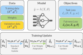
Figure 1: An overview of the FORML algorithm, which optimizes sample weights $w$ and model parameters $\theta$ using the meta-learning paradigm.

In this work, we propose Fairness Optimized Reweighting via Meta-Learning (FORML), an algorithm that directly optimizes both fairness and predictive performance. We follow the learning-to-learn (meta-learning) paradigm (Andrychowicz et al., 2016; Finn et al., 2017; Lake et al., 2015; Ren et al., 2018; Thrun and Pratt, 2012) and jointly learn a weight for each sample in the training set and the model parameters by optimizing for the given test metric and a fairness criteria over a held-out exemplar set, which incorporates data importance into optimization. At a high-level, our algorithm (1) optimizes model parameters via a weighted loss objective, and (2) optimizes a global set of sample weights using a given fairness metric over the exemplar set. An overview of the gradient rules of the algorithm are given in Figure 1. Learning sample weights over an exemplar set helps adapt the model to the fairness metric similar to how the model may be evaluated at test time, allows any practitioner to define fairness non-parametrically, and improves label efficiency as held-out validation sets are typically much smaller than the training data set where attribute labels are needed.

We experiment with image recognition datasets and demonstrate that our approach reduces fairness violations (measured by equality of opportunity) by improving worst group performance without harming overall performance. FORML does not simply learn to reweight based on the number of samples as we see reduced fairness violations even when samples are uniformly distributed across groups, but on the importance of data points to the fairness criteria. Further, FORML improves performance in noisy label settings, and FORML can be used to remove harmful data samples leading to improved fairness and higher data efficiency.

2 Learning to Reweight Data for Optimizing Fairness

Consider a dataset $\mathcal{D}=\{(x^{(i)},y^{(i)},a^{(i)})\mid 1\leq i\leq N\}$, where $x^{(i)}\in\mathcal{X}$ is the input (e.g., images, texts), $y^{(i)}\in\mathcal{Y}$ is the target variable, and $a^{(i)}\in\mathcal{A}$ is the sensitive attribute. Let $D_{\mathcal{T}}$ and $D_{\mathcal{V}}$ denote the train and exemplar sets formed from $\mathcal{D}$, and $(x_{\mathcal{T}}^{(i)},y_{\mathcal{T}}^{(i)},a_{\mathcal{T}}^{(i)})$, $(x_{\mathcal{V}}^{(i)},y_{\mathcal{V}}^{(i)},a_{\mathcal{V}}^{(i)})$ be samples from $D_{\mathcal{T}}$ and $D_{\mathcal{V}}$ respectively. Let $h(x;\theta)\in\mathcal{H}$ be a classifier parameterized by model parameters $\theta$. The main objective is to learn parameters of $h$ that minimize the expected loss: $\theta^{*}=\underset{\theta}{\operatorname*{arg\,min}}\underset{(x^{(i)},y^{(i)},a^{(i)})\sim D_{\mathcal{T}}}{\sum}\mathcal{L}_{c}(h(x^{(i)};\theta),y^{(i)}).$

Improving fairness with minimal impact on accuracy can be formulated as a constrained optimization problem that depends on fairness violation thresholds $\epsilon_{i}$:

$$\theta^{*}= \operatorname*{arg\,min}_{\theta}\sum_{(x^{(i)},y^{(i)},a^{(i)})\sim D_{\mathcal{T}}}\mathcal{L}_{c}(h(x^{(i)};\theta),y^{(i)})$$ (1)

$$\ s.t.\sum_{(x^{(i)},y^{(i)},a^{(i)})\sim D_{\mathcal{T}}}\mathcal{L}_{f}(h(x^{(i)};\theta),y^{(i)};a^{(i)})\leq\epsilon_{i}.$$

Classical algorithms for solving the penalized objective are based on the basic differential multiplier method (Platt and Barr, 1987), which defines a gradient update rule for both model parameters and the weight parameters. Gradient-based approaches to hyper-parameter optimization have also been proposed in (Bengio, 2000).

Constrained optimization with Lagrangians have been studied more recently for fairness (Cotter et al., 2019a, b). Recent work studied Equation 1 in the context of label bias and proposed an iterative reweighting algorithm based on the fairness violation on the training set (Jiang and Nachum, 2020). Other work demonstrated that optimizing model parameters over a given evaluation metric is equivalent to optimizing over an example weighted loss (Zhao et al., 2019).

An alternative view for constrained optimization of (Jiang and Nachum, 2020) is that the model is adapted by the training sample weights (learned through the constraint) to handle new tasks where the constraint is enforced. Such an approach is typically handled well by meta-learning optimization algorithms (Fallah et al., 2021; Finn et al., 2017). We follow a similar procedure to MAML adaptation algorithms (Finn et al., 2017; Ren et al., 2018) and consider a two-step procedure similar to that of (Jiang and Nachum, 2020). We propose an iterative optimization procedure, where the model parameters $\theta_{t+1}$ and sample weights $w_{t+1}$ at the $t$th timestep are jointly optimized according to the learned weighted training objectives:

$$w_{t+1} =\operatorname*{arg\,min}_{w}\mathbb{E}_{(x,y,a)\sim D_{\mathcal{V}}}\left[\mathcal{L}_{f}(h(x;\tilde{\theta}),y;a)\right],$$ (2)

$$\theta_{t+1} =\operatorname*{arg\,min}_{\theta}\mathbb{E}_{(x,y)\sim D_{\mathcal{T}}}\left\langle w_{t+1},\mathcal{L}_{c}(h(x;\theta),y)\right\rangle,$$ (3)

where $\tilde{\theta}=\theta_{t}-\eta_{c}\nabla_{\theta}\mathcal{L}(\theta)\Bigr{|}_{\begin{subarray}{c}\theta=\theta_{t}\end{subarray}}$ is the one gradient descent step update over the training loss. The approach can be summarized as follows: (1) model parameter updates are computed based on the training loss and the model parameters are evaluated on the fair loss on the exemplar set to determine weights that offset the impact to fairness, and (2) model parameters are adapted according to the weight parameters such that the weight parameters do not negatively impact fairness.

Advantages of the proposed meta-learning procedure over a fixed update rule such as (Jiang and Nachum, 2020) and prior meta-learning reweighting methods including (Finn et al., 2017; Ren et al., 2018; Shu et al., 2019) are that FORML (1) incorporates gradient information from the fairness metric to the gradient updates of the model parameters directly adapting the model parameters for fairness, (2) adapts sample weights over exemplar data to better generalize to fairness on the test set by optimizing both (user-defined exemplar) fairness and performance, and (3) learns global weights over training which can be used to learn data importance and difficulty over weights local to a batch.

2.1 Implementation of FORML

Training a model with FORML involves two additional gradient updates over the standard stochastic optimization pipeline. Pseudocode for computation of FORML is given in Algorithm 1 and an overview in Figure 2.

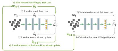
Figure 2: Illustration of the forward and backward passes for the model parameters and training sample weights.

The algorithm is as follows: (1) sample the training set uniformly and exemplar set to ensure a small pre-specified number of samples per class for fairness evaluation, (2) update training example weights by first computing a model update using SGD (Steps 6-8) then updating the example weights based on the gradient of the fairness metric on the exemplar dataset (Steps 9-11), and (3) update the model parameters using the updated sample weights over the original training metric (Steps 12-13) to avoid mixing gradient information from the previous sample weights, resulting in a model which has been adapted to handle both the training metric and fairness metric.

Algorithm 1 FORML: Fairness-Optimized Reweighting via Meta-Learning

1:  Input: $\mathcal{D}_{T}$, $\mathcal{D}_{V}$, $\theta_{0}$, $w_{0}$, $\mathcal{L}_{c}$, $\mathcal{L}_{f}$, $\eta_{c}$, $\eta_{f}$

2:  for $t=0$ to $T-1$ do

3:     for $b=0$ to $B-1$ do

4:        $X_{\mathcal{T}},y_{\mathcal{T}}\leftarrow$ sample($D_{\mathcal{T}}$, $b$),

5:        $X_{\mathcal{V}},y_{\mathcal{V}}\leftarrow$ sample_fair($D_{\mathcal{V}}$, $b$)

6:        $\hat{y}_{\mathcal{T}}\leftarrow h(X_{\mathcal{T}};\theta_{t})$

7:        $\delta_{c}=\sum_{i=1}^{n}\nabla_{\theta_{t}}\left[\frac{exp(w_{t}^{(i)})}{\sum_{j}{exp(w_{t}^{(j)}})}\mathcal{L}_{c}\left(y^{(i)}_{\mathcal{T}},\hat{y}^{(i)}_{\mathcal{T}}\right)\right]$

8:        $\tilde{\theta}_{t}\leftarrow\theta_{t}-\eta_{c}\delta_{c}$

9:        $\hat{y}_{\mathcal{V}}\leftarrow h(X_{\mathcal{V}};\tilde{\theta}_{t})$

10:        $\delta_{f}=\sum_{i=1}^{n}\nabla_{w_{t}}\left[\mathcal{L}_{f}\left(y^{(i)}_{\mathcal{V}},\hat{y}^{(i)}_{\mathcal{V}}\right)\right]$

11:        $w_{t+1}\leftarrow w_{t}-\eta_{f}\delta_{f}$

12:        ${\tilde{\delta}_{c}}=\sum_{i=1}^{n}\nabla_{\theta_{t}}\left[\frac{exp(w_{t+1}^{(i)})}{\sum_{j}{exp(w_{t+1}^{(j)}})}\mathcal{L}_{c}\left(y^{(i)}_{\mathcal{T}},\hat{y}^{(i)}_{\mathcal{T}}\right)\right]$

13:        $\theta_{t+1}\leftarrow\theta_{t}-\eta_{f}{\tilde{\delta}_{c}}$

14:     end for

15:  end for

3 Image Classification Results

We experiments on image recognition datasets to demonstrate FORML mitigates bias in datasets. In all experiments, FORML reduces fairness violations while maintaining accuracy. While other works further reduce fairness violations as in (Jiang and Nachum, 2020), doing so typically results in a decrease in accuracy and is different from our aims.

3.1 Experimental Setup

We compare FORML with prior weighting schemes for improving fairness and robustness, including static weighting strategies: uniform, random, and class-balanced weighting (Cui et al., 2019), and learned weighting strategies: LB (Jiang and Nachum, 2020), MOEW (Zhao et al., 2019), and MWN (Shu et al., 2019). In our experiments, we take the exemplar set as the pre-defined validation set if the dataset has one, or create one by sampling uniformly (by attribute) from the training set.

3.2 CIFAR Experiments

In this section, we evaluate FORML using CIFAR-10 and CIFAR-100, and investigate whether FORML learns training sample weights that improve fairness. For these experiments, there is no pre-defined sensitive attribute, therefore we use the class label as the sensitive attribute, and the objective is to achieve equal classification performance across classes reported as TPRD.

Method	TPRD (%) $\downarrow$	maxFNR (%) $\downarrow$	Accuracy (%) $\uparrow$
Uniform / Proportion	$8.79\pm 0.14$	$10.80\pm 0.14$	$\bm{95.25\pm 0.03}$
Random	$11.22\pm 0.15$	$13.84\pm 0.85$	$93.77\pm 0.04$
MOEW	$23.08\pm 0.26$	$30.88\pm 0.23$	$83.072\pm 0.03$
MWN	$9.0\pm 0.15$	$11.17\pm 0.14$	$95.10\pm 0.03$
LB	$8.68\pm 0.15$	$10.73\pm 0.14$	$95.21\pm 0.03$
FORML	$\bm{7.97\pm 0.12}$	$\bm{10.36\pm 0.17}$	$95.20\pm 0.03$

Table 1: Fairness metrics: True Positive Rate Disparity (TPRD), Maximum False Negative Rate (maxFNR), and test accuracy for ResNet-18 on CIFAR-10. The means and standard errors are from 30 runs.

We train a ResNet-18 architecture (He et al., 2016) and summarize results in Table 1. Neither random nor MOEW are able to perform competitively with other methods, and FORML achieves $\sim 1\%$ improvement (a relative performance gain of $\sim 10\%$) over uniform and label bias on CIFAR-10.

Method	TPRD (%) $\downarrow$	maxFNR (%) $\downarrow$	Accuracy (%) $\uparrow$
Uniform / Proportion	$46.27\pm 0.46$	$49.29\pm 0.43$	$\bm{77.80\pm 0.06}$
Random	$50.56\pm 0.43$	$55.56\pm 0.38$	$72.54\pm 0.08$
MOEW	$67.2\pm 0.72$	$80.6\pm 0.68$	$53.94\pm 0.03$
MWN	$45.83\pm 0.46$	$49.13\pm 0.45$	$77.62\pm 0.05$
LB	$45.87\pm 0.52$	$49.17\pm 0.46$	$77.73\pm 0.05$
FORML	$\bm{45.17\pm 0.35}$	$\bm{48.80\pm 0.32}$	$77.51\pm 0.08$

Table 2: Performance with ResNet-18 on CIFAR-100. The means and standard errors are from 30 runs.

For CIFAR-100, we see a similar trend in Table 2, where only FORML is able to outperform the uniform training method while simultaneously maintaining accuracy.

3.3 Celeb-A Experiments

We train a ResNet-18 architecture (He et al., 2016) to predict the binary attribute “Attractive”. The sensitive attribute is gender denoted by “Male”. For Celeb-A, we use the pre-defined train, val, test split and compare models at the epoch with the highest validation accuracy during training. Metrics are reported over the test set in Table 3.

Method	TPRD (%) $\downarrow$	maxFNR (%) $\downarrow$	Accuracy (%) $\uparrow$
Uniform	$24.91\pm 1.67$	$36.51\pm 1.78$	$81.72\pm 0.04$
Random	$24.52\pm 1.40$	$34.59\pm 1.68$	$80.63\pm 0.14$
Proportion	$23.44\pm 1.71$	$34.68\pm 1.79$	$81.71\pm 0.10$
LB	$24.63\pm 1.62$	$36.94\pm 2.63$	$\bm{81.91\pm 0.07}$
FORML	$\bm{22.32\pm 1.7}$	$\bm{31.14\pm 1.87}$	$81.63\pm 0.24$

Table 3: Celeb-A attribute prediction performance with “Attractive” target attribute and “Gender” protected attribute. The means and standard errors are from 5 runs.

Both proportional reweighting based on sensitive attribute and random weightings perform better than uniform weighting on maxFNR and proportional reweighting improves TPRD by 1%, however the label bias approach offers no advantage over uniform training. In contrast, FORML achieves a reduction of $\sim 2\%$ (a relative performance gain of $\sim 10\%$) on the fairness violation (TPRD), and a reduction of $\sim 5\%$ in maxFNR (a relative performance gain of $\sim 15\%$), while retaining accuracy.

4 Data Robustness and Condensation

4.1 Mislabeled Data in MNIST

We investigate the performance of FORML with mislabeled data, where the objective is to learn data weights and ignore wrongly labeled data. To simulate this setup, we take the MNIST dataset and randomly change $20\%$ of the training data labels to “$2$”, as in (Jiang and Nachum, 2020). Based on the results in Table 4, FORML achieves higher accuracy and reduces fairness violation over training with uniform weighting and label bias weightings. In the supplementary material, we compared the ratio of weighted loss of samples labeled “2” to other samples demonstrating FORML learns less from mislabeled samples than uniform weighting.

Method	TPRD (%) $\downarrow$	maxFNR (%) $\downarrow$	Accuracy (%) $\uparrow$
Uniform (clean data)	$5.21\pm 0.40$	$6.12\pm 0.40$	$97.16\pm 0.12$
Uniform	$8.59\pm 0.91$	$10.00\pm 0.89$	$95.24\pm 0.36$
LB	$7.71\pm 0.76$	$9.05\pm 0.76$	$95.52\pm 0.27$
FORML	$\bm{6.93\pm 0.79}$	$\bm{8.22\pm 0.83}$	$\bm{95.90\pm 0.21}$

Table 4: Performance of a two-hidden-layer MLP on the MNIST dataset with 20% mislabeled data. The means and standard errors are reported over 10 runs.

4.2 Using Data Weights to Build Fair Datasets

FORML improves fairness by identifying representative samples and reducing impact of harmful samples during training. We extend this analysis and investigate if FORML can post-hoc condense datasets yielding a more fair dataset. Specifically, we train a model with FORML using an exemplar set of $1000$ samples with the lowest number of forgetting events (Toneva et al., 2018). We then remove 10% of the training samples with the lowest normalized weighted loss, computed using an exponential moving average (EMA) over training epochs. Using a moving average incorporates weight impact over all of training rather than only considering the weights at the end of training.

Method	TPRD (%) $\downarrow$	maxFNR (%) $\downarrow$	Accuracy (%) $\uparrow$
Uniform 50k	$46.0\pm 0.85$	$49.6\pm 0.92$	$\bm{77.74\pm 0.18}$
Random 45k	$46.8\pm 0.33$	$50.0\pm 0.49$	$76.7\pm 0.09$
FORML 45k	$\bm{43.8\pm 0.52}$	$\bm{47.6\pm 0.36}$	$77.50\pm 0.04$

Table 5: Performance of ResNet-18 re-training on CIFAR-100 with data removal. The means and standard errors are reported over 5 runs.

To demonstrate performance with the sub-sampled dataset, we re-train the model using standard training with the sub-sampled dataset; results are summarized in Table 5 and indicate that on CIFAR-100, removing samples based on the weighted EMA of the loss performs similarly and reduces fairness violation over training with the full dataset. Training on the sub-sampled dataset also leads to better results than a model that has been trained on a random subset of the same size. This indicates that FORML weights can build fairer datasets through removing harmful samples.

5 Conclusion

In this work, we present FORML, an algorithm for dynamically reweighting data to train fair networks, and identify and mitigate bias from erroneous or over-represented samples. FORML has several benefits: it is simple to implement by making small modifications in training, and requires neither data pre-processing nor post-processing of the model outputs. Further, FORML is a data-centric method that improves fairness based on the dataset and is agnostic to the model and fairness metric, extending beyond classification. We believe this work is a step towards creating fairer models without sacrificing accuracy by better leveraging data.

Appendix A FORML Hyperparameters: Sensitivity and Variations

A.1 FORML Hyperparameters

CIFAR: For CIFAR-10/100, we train a ResNet-18 architecture [He et al., 2016] using SGD with Nesterov momentum $\gamma=0.9$ and batch size of $128$. We set the initial learning rate to $\eta_{c}=0.1$ and decay by $0.1$ at the $60$^th, $120$^th, and $160$^th epochs and train for a total of $200$ epochs. We also penalize the model parameters with weight decay at $5e-4$. For both CIFAR-10/100, we use standard data augmentations (normalization, random horizontal flip, translation by up to 4 pixels). To learn the training sample weights in FORML, we use SGD with the same learning rate as the model parameter learning rate and minimize the max loss discrepancy. For MOEW on CIFAR-10 we used twenty batches for learning the weight function parameters and fifty batches on CIFAR-100. Both MOEW and FORML use a held-out validation set of 5000 samples for learning weights and maintains a minimum of 3 samples per class per batch.

Celeb-A: For Celeb-A, we train a ResNet-18 architecture [He et al., 2016] to predict the binary attribute “Attractive” given images of faces. The sensitive attribute is gender denoted by “Male” in the dataset. The model is trained using Adam optimizer and batch size of $256$. We set the initial learning rate to $\eta_{c}=0.001$ and train for a total of $10$ epochs. For pre-processing the images, we center-crop and resize to size $128\times 128$ and normalize. To learn the training sample weights in FORML, we use SGD with the same learning rate as the model parameter learning rate and minimize the mean loss discrepancy. The validation set maintains a minimum of 20 samples per class per batch for FORML. For the proportion weighting, we take the number of samples according to the sensitive attribute because the number of samples in each group for the target attribute “Attractive” are nearly identical at $51.4\%$ in the training set and we seek to reduce fairness violations in the sensitive attribute “Male” in the dataset. For this dataset, we use the pre-defined train, val, test split and compare models at the epoch with the highest validation accuracy during training. Metrics are reported over the test set

MNIST: For the corrupt-label MNIST experiment, a two hidden layer network with ReLU activations is used. For all methods, we select $5$k samples randomly from the training set for validation and use early stopping to prevent overfitting to the corrupt labels. We use the same training hyperparameters as in [Jiang and Nachum, 2020].

A.2 FORML Variations

We conduct ablation studies on the Celeb-A dataset to determine the impact of different hyperparameters and settings in FORML. In the main paper, we use the best performing hyperparameters that also reduce the number of hyperparameters needed to tune (i.e. maintaining the same learning rate, and only reported results with two meta-loss functions, although there are many others that are compatible with FORML).

Reverse and Adversarial comparisons: Our algorithm shares many similarities with the Lagrange multipliers and basic differentiable multipliers method (BDMM) algorithms [Platt and Barr, 1987], which have been applied for constrained optimization problems and in recent work for fairness [Cotter et al., 2019a, Jiang and Nachum, 2020]. In the BDMM algorithm, it is argued that standard gradient descent for the constraint in Lagrange multipliers does not work and instead the reverse sign should be applied [Platt and Barr, 1987]. We experiment with both a reverse sign in the update for the model parameters in the first update, as well as for the weights of the model and report results in Table 6 and Table 7. Results indicate that FORML performs better when using the reverse update on the model parameters, but the reverse update on the sample weights has little effect. While results are slightly higher for the test accuracy, TPRD on the validation set was on average $1\%$ lower for the reverse update on the sample weights. Thus our algorithm in the main paper uses a reverse update for the model parameters, and not for the sample weights indicating some differences from the BDMM algorithm.

Method	TPRD (%) $\downarrow$	maxFNR (%) $\downarrow$	Accuracy (%) $\uparrow$
No Reverse	$22.80\pm 3.88$	$37.35\pm 7.55$	$\bm{79.99\pm 1.11}$
Reverse	$\bm{20.41\pm 3.34}$	$\bm{33.89\pm 8.34}$	$79.48\pm 0.82$

Table 6: Testing the model with a reverse update for the model parameters by comparing the True Positive Rate Disparity (TPRD), Maximum False Negative Rate (maxFNR), and test accuracy on Celeb-A. The means and standard errors are from 5 runs. $\downarrow$ denotes lower values are better. $\uparrow$ denotes higher values are better.

Method	TPRD (%) $\downarrow$	maxFNR (%) $\downarrow$	Accuracy (%) $\uparrow$
No Reverse	$\bm{20.41\pm 3.34}$	$33.89\pm 8.34$	$79.48\pm 0.82$
Reverse	$20.45\pm 2.44$	$\bm{33.32\pm 6.4}8$	$\bm{80.37\pm 0.57}$

Table 7: Testing the model with a reverse update for the model parameters by comparing the True Positive Rate Disparity (TPRD), Maximum False Negative Rate (maxFNR), and test accuracy on Celeb-A. The means and standard errors are from 5 runs. $\downarrow$ denotes lower values are better. $\uparrow$ denotes higher values are better.

Meta Loss Variations: In Section 3, the meta-loss optimized over the validation set is either the MaxLossD or the MeanLossD which generally perform similarly. We demonstrate the advantage of using a loss oriented for fairness in Table 8 by comparing with the cross entropy loss. We find that using MaxLossD and MeanLossD lower the fairness violation, but marginally lowers accuracy; whereas using cross entropy increases accuracy slightly but does not lower the fairness violation with respect to baseline performance from Table 3.

Method	TPRD (%) $\downarrow$	maxFNR (%) $\downarrow$	Accuracy (%) $\uparrow$
MaxLossD	$20.85\pm 2.88$	$37.66\pm 7.96$	$79.41\pm 0.59$
MeanLossD	$\bm{20.41\pm 3.34}$	$\bm{33.89\pm 8.34}$	$79.48\pm 0.82$
Cross Entropy	$24.70\pm 2.74$	$38.87\pm 4.76$	$\bm{81.08\pm 0.48}$

Table 8: Testing the model with cross entropy as the meta-loss by comparing the True Positive Rate Disparity (TPRD), Maximum False Negative Rate (maxFNR), and test accuracy on Celeb-A. The means and standard errors are from 5 runs. $\downarrow$ denotes lower values are better. $\uparrow$ denotes higher values are better.

Sample Weight Variations: In Section 3, the weights are directly multiplied to balance the loss. However, other variations of weights could be applied to balance the loss such as weights on the logits, or a different function of the weight parameters to enforce different behavior. Here, we explore a reweighting based on the logits, and a weighting based on the $L_{1}$ penalty that encourages sparsity of the weights by forcing weights that are too large to zero; we denote this weighting as the inverse square $L_{1}$ [Seto et al., 2021]. Both are compared with the baseline of directly multiplying the learned sample weights with the sample loss, and results reported in Table 9 indicate that the baseline reweighting performs best across all metrics.

Method	TPRD (%) $\downarrow$	maxFNR (%) $\downarrow$	Accuracy (%) $\uparrow$
Baseline	$\bm{18.91\pm 1.16}$	$\bm{28.57\pm 2.27}$	$\bm{80.91\pm 0.30}$
Logits	$25.32\pm 2.36$	$43.81\pm 5.96$	$80.65\pm 0.58$
Inverse Sq. $L_{1}$	$24.52\pm 3.67$	$44.08\pm 9.50$	$78.90\pm 1.02$

Table 9: Testing the model with different methods for applying weights by comparing the True Positive Rate Disparity (TPRD), Maximum False Negative Rate (maxFNR), and test accuracy on Celeb-A. The means and standard errors are from 5 runs. $\downarrow$ denotes lower values are better. $\uparrow$ denotes higher values are better.

Appendix B Alternative CelebA Tasks

In addition to the task of predicting the “Attractive” attribute with gender (denoted “Male”) as the sensitive attribute, we also experiment with different tasks and sensitive attributes to test robustness of FORML to different tasks. We change the sensitive attribute to the “Pale Skin” attribute (color), and the prediction task to the “Young” attribute. Accuracy on this task is higher than for the “Attractive” attribute, and as such the fairness violation is lower. Nonetheless, we report in Table 10 that FORML is able to reduce fairness violations over uniform weighting.

Method	TPRD (%) $\downarrow$	maxFNR (%) $\downarrow$	Accuracy (%) $\uparrow$
Uniform	$2.64\pm 0.46$	$5.36\pm 0.25$	$\bm{87.62\pm 0.09}$
FORML	$\bm{2.51\pm 0.43}$	$\bm{4.64\pm 0.84}$	$87.07\pm 0.22$

Table 10: Evaluating FORML for predicting “Young” subject to the sensitive attribute color (“Pale Skin”) according to the metrics: True Positive Rate Disparity (TPRD), Maximum False Negative Rate (maxFNR), and test accuracy on Celeb-A. The means and standard errors are from 5 runs. $\downarrow$ denotes lower values are better. $\uparrow$ denotes higher values are better.

Appendix C More on the Normalized Loss for Reducing Overfitting to Corrupt Labels

In Section 4.1, FORML is tested in the robustness setting with incorrect labels. We further explore how training with FORML improves performance by examining the loss for each sample over epochs during training. The objective of this analysis is to investigate how the loss differs for the model trained with FORML, and how this leads to improvement on the test set.

We compute an exponential moving average (EMA) on the loss and compare the average EMA loss for samples with label “2” to samples with another label. As expected, since many of the samples have an incorrect label “2”, the loss for samples with label “2” is higher in both a model trained with uniform weights and the model trained with FORML. For a model with uniform weights, the ratio of the losses for label “2” samples to other samples is $2.9$. In comparison, the model trained with FORML has a ratio of $2.61$, a relative decrease of $10\%$. As the accuracy for both models in predicting samples with label “2” are relatively similar, we can conclude it is likely that the weights learned by FORML are reducing the model’s ability to overfit to the incorrect labels leading to better performance on the test set.

References

- Andrychowicz et al. [2016] Marcin Andrychowicz, Misha Denil, Sergio Gomez, Matthew W Hoffman, David Pfau, Tom Schaul, Brendan Shillingford, and Nando De Freitas. Learning to learn by gradient descent by gradient descent. In Advances in neural information processing systems, pages 3981–3989, 2016.
- Bengio [2000] Yoshua Bengio. Gradient-based optimization of hyperparameters. Neural Comput., 12(8):1889–1900, 2000.
- Cotter et al. [2019a] Andrew Cotter, Heinrich Jiang, Maya R Gupta, Serena Wang, Taman Narayan, Seungil You, and Karthik Sridharan. Optimization with non-differentiable constraints with applications to fairness, recall, churn, and other goals. J. Mach. Learn. Res., 20(172):1–59, 2019a.
- Cotter et al. [2019b] Andrew Cotter, Heinrich Jiang, and Karthik Sridharan. Two-player games for efficient non-convex constrained optimization. In Algorithmic Learning Theory, pages 300–332. PMLR, 2019b.
- Cui et al. [2019] Yin Cui, Menglin Jia, Tsung-Yi Lin, Yang Song, and Serge Belongie. Class-balanced loss based on effective number of samples. In Proceedings of the IEEE/CVF conference on Computer Vision and Pattern Recognition, CVPR, pages 9268–9277, 2019.
- Devlin et al. [2019] Jacob Devlin, Ming-Wei Chang, Kenton Lee, and Kristina Toutanova. BERT: pre-training of deep bidirectional transformers for language understanding. In Proceedings of the 2019 Conference of the North American Chapter of the Association for Computational Linguistics: Human Language Technologies, NAACL-HLT, pages 4171–4186. Association for Computational Linguistics, 2019.
- Dong et al. [2017] Qi Dong, Shaogang Gong, and Xiatian Zhu. Class rectification hard mining for imbalanced deep learning. In Proceedings of the IEEE International Conference on Computer Vision, pages 1851–1860, 2017.
- Esteva et al. [2019] Andre Esteva, Alexandre Robicquet, Bharath Ramsundar, Volodymyr Kuleshov, Mark DePristo, Katherine Chou, Claire Cui, Greg Corrado, Sebastian Thrun, and Jeff Dean. A guide to deep learning in healthcare. Nature Medicine, 25(1):24–29, 2019.
- Fallah et al. [2021] Alireza Fallah, Aryan Mokhtari, and Asuman Ozdaglar. Generalization of model-agnostic meta-learning algorithms: Recurring and unseen tasks. arXiv preprint arXiv:2102.03832, 2021.
- Fan et al. [2018] Yang Fan, Fei Tian, Tao Qin, Xiang-Yang Li, and Tie-Yan Liu. Learning to teach. In International Conference on Learning Representations, 2018.
- Finn et al. [2017] Chelsea Finn, Pieter Abbeel, and Sergey Levine. Model-agnostic meta-learning for fast adaptation of deep networks. In International Conference on Machine Learning, pages 1126–1135. PMLR, 2017.
- Hardt et al. [2016] Moritz Hardt, Eric Price, and Nati Srebro. Equality of opportunity in supervised learning. In Advances in Neural Information Processing Systems 29, pages 3315–3323, 2016.
- He et al. [2016] Kaiming He, Xiangyu Zhang, Shaoqing Ren, and Jian Sun. Deep residual learning for image recognition. In Proceedings of the IEEE conference on computer vision and pattern recognition, pages 770–778, 2016.
- Hinton et al. [2012] Geoffrey Hinton, Li Deng, Dong Yu, George E Dahl, Abdel-rahman Mohamed, Navdeep Jaitly, Andrew Senior, Vincent Vanhoucke, Patrick Nguyen, Tara N Sainath, et al. Deep neural networks for acoustic modeling in speech recognition: The shared views of four research groups. IEEE Signal processing magazine, 29(6):82–97, 2012.
- Jiang and Nachum [2020] Heinrich Jiang and Ofir Nachum. Identifying and correcting label bias in machine learning. In The 23rd International Conference on Artificial Intelligence and Statistics, AISTATS, pages 702–712. PMLR, 2020.
- Jiang et al. [2018] Lu Jiang, Zhengyuan Zhou, Thomas Leung, Li-Jia Li, and Li Fei-Fei. Mentornet: Learning data-driven curriculum for very deep neural networks on corrupted labels. In International Conference on Machine Learning, pages 2304–2313. PMLR, 2018.
- Kahn and Marshall [1953] Herman Kahn and Andy W Marshall. Methods of reducing sample size in monte carlo computations. Journal of the Operations Research Society of America, 1(5):263–278, 1953.
- Krizhevsky et al. [2012] Alex Krizhevsky, Ilya Sutskever, and Geoffrey E. Hinton. Imagenet classification with deep convolutional neural networks. In Advances in Neural Information Processing Systems, pages 1106–1114, 2012.
- Kumar et al. [2010] M Kumar, Benjamin Packer, and Daphne Koller. Self-paced learning for latent variable models. Advances in neural information processing systems, 23:1189–1197, 2010.
- Lahoti et al. [2020] Preethi Lahoti, Alex Beutel, Jilin Chen, Kang Lee, Flavien Prost, Nithum Thain, Xuezhi Wang, and Ed H Chi. Fairness without demographics through adversarially reweighted learning. In Advances in Neural Information Processing Systems 33, 2020.
- Lake et al. [2015] Brenden M Lake, Ruslan Salakhutdinov, and Joshua B Tenenbaum. Human-level concept learning through probabilistic program induction. Science, 350(6266):1332–1338, 2015.
- Lin et al. [2017] Tsung-Yi Lin, Priya Goyal, Ross Girshick, Kaiming He, and Piotr Dollár. Focal loss for dense object detection. In Proceedings of the IEEE International Conference on Computer Vision, ICCV, pages 2980–2988, 2017.
- Malisiewicz et al. [2011] Tomasz Malisiewicz, Abhinav Gupta, and Alexei A Efros. Ensemble of exemplar-svms for object detection and beyond. In 2011 International conference on computer vision, pages 89–96. IEEE, 2011.
- Petrović et al. [2020] Andrija Petrović, Mladen Nikolić, Sandro Radovanović, Boris Delibašić, and Miloš Jovanović. Fair: Fair adversarial instance re-weighting. arXiv preprint arXiv:2011.07495, 2020.
- Platt and Barr [1987] John C Platt and Alan H Barr. Constrained differential optimization. In Proceedings of the 1987 International Conference on Neural Information Processing Systems, pages 612–621, 1987.
- Ren et al. [2018] Mengye Ren, Wenyuan Zeng, Bin Yang, and Raquel Urtasun. Learning to reweight examples for robust deep learning. In Proceedings of the 35th International Conference on Machine Learning, ICML, pages 4334–4343. PMLR, 2018.
- Roh et al. [2021] Yuji Roh, Kangwook Lee, Steven Euijong Whang, and Changho Suh. Sample selection for fair and robust training. In Thirty-Fifth Conference on Neural Information Processing Systems, 2021.
- Saxena et al. [2019] Shreyas Saxena, Oncel Tuzel, and Dennis DeCoste. Data parameters: A new family of parameters for learning a differentiable curriculum. In Advances in Neural Information Processing Systems, pages 11093–11103, 2019.
- Seto et al. [2021] Skyler Seto, Martin T Wells, and Wenyu Zhang. Halo: Learning to prune neural networks with shrinkage. In Proceedings of the 2021 SIAM International Conference on Data Mining (SDM), pages 558–566. SIAM, 2021.
- Shu et al. [2019] Jun Shu, Qi Xie, Lixuan Yi, Qian Zhao, Sanping Zhou, Zongben Xu, and Deyu Meng. Meta-weight-net: Learning an explicit mapping for sample weighting. Advances in Neural Information Processing Systems, 32:1919–1930, 2019.
- Thrun and Pratt [2012] Sebastian Thrun and Lorien Pratt. Learning to learn. Springer Science & Business Media, 2012.
- Toneva et al. [2018] Mariya Toneva, Alessandro Sordoni, Remi Tachet des Combes, Adam Trischler, Yoshua Bengio, and Geoffrey J Gordon. An empirical study of example forgetting during deep neural network learning. In International Conference on Learning Representations, 2018.
- Vyas et al. [2020] Nidhi Vyas, Shreyas Saxena, and Thomas Voice. Learning soft labels via meta learning. arXiv preprint arXiv:2009.09496, 2020.
- Wu et al. [2018] Lijun Wu, Fei Tian, Yingce Xia, Yang Fan, Tao Qin, Jian-Huang Lai, and Tie-Yan Liu. Learning to teach with dynamic loss functions. In NeurIPS, 2018.
- Zadrozny [2004] Bianca Zadrozny. Learning and evaluating classifiers under sample selection bias. In Proceedings of the twenty-first international conference on Machine learning, page 114, 2004.
- Zhao et al. [2019] Sen Zhao, Mahdi Milani Fard, Harikrishna Narasimhan, and Maya R. Gupta. Metric-optimized example weights. In Proceedings of the 36th International Conference on Machine Learning, ICML, volume 97 of Proceedings of Machine Learning Research, pages 7533–7542. PMLR, 2019.