around Smale’s 14th problem

Abstract.

We consider the Lorenz equations, a system of three dimensional ordinary differential equations modeling atmospheric convection. As the equations are chaotic and hard to study, a simpler “geometric model” has been introduced in the seventies. One of the classical problems in dynamical systems is to relate the original equations to the simplified geometric model. This has been achieved numerically by Tucker [24]. Here we show that for a different parameter we can prove the relation to the geometric model analytically, by elementary geometric means.

1. Introduction

In 1963 Edward Lorenz, a mathematician and meteorologist, introduced a simplified model for heat convention [17]:

(1) $$\left\{\begin{array}[]{rlr}\dot{x}(t)&=\sigma(y-x)\\ \dot{y}(t)&=\rho x-y-xz\\ \dot{z}(t)&=xy-\beta z\end{array}\right.$$

This system has been extensively studied over the last decades, being the first system to demonstrate chaos in a deterministic low dimensional setting and serving as a paradigm for chaotic systems [14]. It arises in many different mathematical models of chaotic systems and has been studied especially at the classical parameter values $\rho=28,\sigma=10,\beta=\frac{8}{3}$ which were those originally studied by Lorenz.

At these parameter values, the three-dimensional motion given by the Lorenz equations (1) converges almost always onto its famous butterfly-shaped strange attractor. Although this is easily seen to be the case by running any ODE solver, there is no analytical proof for it.

In the seventies, a simpler dynamical system called the geometric Lorenz model, was developed [15, 1]. The geometric model shares by design much of the characteristics of the equations, as it also displays a butterfly-shaped strange attractor. At the same time, the geometric model is susceptible to analytic study and it can be proven to be chaotic in a specific sense. i.e., one can prove both geometric properties on the shape of the attractor and the orbits within it, and statistical properties about the rate in which orbits are “mixed”. For example, the attractor has a central limit theorem [16] and exponential decay of correlations [3]. The periodic orbits in the geometric model, which are called “Lorenz knots”, have been studied topologically by Williams [25] and Birman and Williams [6] (see also [12, 5]) and have a number of surprising knot properties.

In 1998 Steve Smale compiled a list of 18 major unsolved problems in mathematics  [21], many of which are still unresolved. His 14th problem asks whether the Lorenz system at the classical parameters given above can be proven to be equivalent to the geometric model. This has been answered by Warwick Tucker [24], via a rigorous numerical proof. Tucker’s proof implies in particular that the Lorenz equations indeed possess a butterfly strange attractor.

An astounding result of Ghys [13] is that the set of Lorenz knots also arise as the set of periodic orbits for a very different flow; the geodesic flow on the modular surface. The modular geodesic flow is a hyperbolic flow arising from number theory. It is also chaotic but its geometric and statistical properties can more readily be proven. The modular flow is also three dimensional but is not defined on the entire three dimensional space. One must exclude a one dimensional set that is a knot called the trefoil knot, which is the knot depicted in purple in Figure 1, connecting to infinity. In knot theory, the trefoil is the simplest nontrivial knot. The Lorenz equations have three singular points where the vector field defining the equations vanishes. Thus, one may search for “heteroclinic connections”, i.e. regular orbits that connect two of these singular points. In the Lorenz equations it is well known numerically that there exist points in parameter space (called T-points) for which there is a heteroclinic connection connecting the origin to one of the singularities in the center of the butterfly wings. Due to the symmetry $(x,y,z)\mapsto(-x,-y,z)$ for the equations, it follows that in these parameters there is also a second heteroclinic connection and thus all three singular points are connected there [19, 2, 9]. It has been suggested by the author in [20] that this heteroclinic connection can be continued to an invariant knot passing also through infinity. For the first T-point at $\rho_{0}\approx 30.8680,\sigma_{0}\approx 10.1673$ and $\beta_{0}=\frac{8}{3}$, the invariant knot is a trefoil knot, depicted in Figure 1

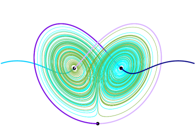
Figure 1. The trefoil knot at the first T-point, see also [11].

In an attempt to explain the relation between the equations and the geometric model and the modular geodesic flow, Christian Bonatti and the author have constructed an extension of the geometric model [7], which for some parameter has an invariant trefoil shaped heteroclinic connection just like the original equations.

Our main theorem is an approximate answer to Smale’s problem. It is an analytical proof that there indeed exists a T-point parameter as observed numerically, and that at this T-point the Lorenz equations can be continuously deformed to the geometric model.

Theorem 1.1.

There exists a parameter value for the Lorenz equations for which a trefoil-shaped heteroclinic connection exists. At this parameter value, the flow defined by the Lorenz equations is isotopic to the extended geometric model.

The main tool is the existence of a convenient cross section for the flow, which allows us to establish the return map corresponds to a symbolic dynamics on two symbols. Deformations of flows in general need not behave nicely with respect to the dynamics. Our second result is to show that the deformation of the Lorenz equations to the geometric model cannot create new periodic orbits, and thus we know that anything we can prove for the geometric model exists also for the original equations. This is done using the section in order to apply methods from two dimensional dynamics [23, 8, 4].

Theorem 1.2.

Any periodic orbit in the geometric model is isotopic to a periodic orbit for the Lorenz equations at the T-point.

An immediate corollary of our results above and Ghys’ theorem [13] is thus the following.

Corollary 1.3.

The geodesic flow on the modular surface is the minimal representative to the Lorenz equation at the trefoil T-point. Namely, a periodic geodesic is isotopic to a periodic orbit of the Lorenz equations.

Note that at the classical parameters it follows from Tucker’s proof that any periodic orbit for the Lorenz equation is isotopic to a modular geodesic, however, not every geodesic appears. Thus our theorem is in a sense a converse to Ghys’.

Acknowledgments

The author wishes to thank Lilya and Misha Lyubich, Omri Sarig, Andrey Shilnikov and Gershon Wolansky for helpful discussions.

2. The existence of a heteroclinic trefoil

In this section we prove the existence of a trefoil heteroclinic connection passing through all four singular points for some point in the parameter space. The first step in the proof is establishing the existence of a global cross section, and the second is a winding number argument.

The cross section we use is modified from the one commonly used in numerical studies which has a constant $z$ coordinate, and is reminiscent of Sparrow’s study of the local $z$ maxima along orbits [22]. It remains a section also at parameter values for which the regular section fails to be one.

Proposition 2.1.

There exists an open simply connected domain $A$ of parameters, for which at any point $(\beta,\sigma,\rho)$ there exists a two dimensional topological rectangle $R\subset\mathbb{R}^{3}$ with interior transverse to the Lorenz flow, so that the forward orbit of any point in $\mathbb{R}^{3}$ that does not limit onto one of the singular points meets $R$.

Proof.

We start by considering the hyperbolic paraboloid

$$\mathcal{P}:=\{xy=\beta z\}$$

Which is the set of points for which $\dot{z}=0$, containing the three singular points. The paraboloid $\mathcal{P}$ divides $\operatorname{\mathbb{R}}^{3}$ into two components, we call the part of $\operatorname{\mathbb{R}}^{3}\setminus\operatorname{\mathcal{P}}$ above the origin the inside and the other component the outside.

For any orbit, its $z$ coordinate decreases while it is on the inside, and increases if and only if it crosses $\operatorname{\mathcal{P}}$ to be on its outside and so on.

A normal to $\operatorname{\mathcal{P}}$ is given by

$$N=(y,x,-\beta).$$

The vector field is tangent to $\operatorname{\mathcal{P}}$ exactly when it is orthogonal to the normal. Taking the inner product of $N$ with the vector field $X=(\dot{x},\dot{y},\dot{z})$ along the paraboloid $\operatorname{\mathcal{P}}$ we obtain

$$N\cdot X=\sigma y^{2}-\sigma xy+\rho x^{2}-xy-\frac{1}{\beta}x^{3}y$$

The equation $N\cdot X=0$ is quadratic in $y$, and thus the set of points $N\cdot X=0$ for which the vector field is tangent to $\operatorname{\mathcal{P}}$ consists of a point at the origin, and of two smooth one dimensional curves which we denote by $\delta_{-}$ and $\delta_{+}$ each containing one of the wing centers.

When $\rho>\frac{(\sigma+1)^{2}}{4\sigma}$ the two dimensional curves are far from the origin and the point at the origin is an isolated solution, while for smaller $\rho$ the two curves have cusps touching the origin. Thus we will restrict our attention from now on to the domain

$${A}=\left\{\beta,\sigma,\rho|\,\beta,\sigma>0,\rho>1,\rho>\frac{(\sigma+1)^{2}}{4\sigma}\right\}.$$

Note that the domain $A$ is simply connected (i.e. any loop in $A$ can be continuously retracted to a point). For any parameter in $A$, the orbits cross $\operatorname{\mathcal{P}}$ to its outside below the two curves $\delta_{-}$ and $\delta_{+}$ and enter the inside above these curves. An example of the regions of entrance to the inside of $\operatorname{\mathcal{P}}$ and exit from it are depicted in Figure 2.

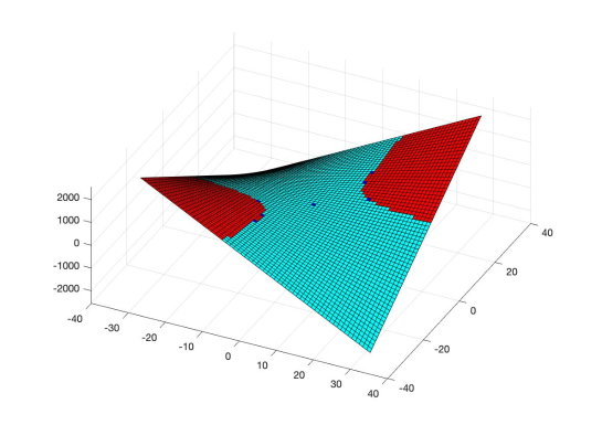
Figure 2. The paraboloid $\operatorname{\mathcal{P}}$ for the classical parameters, with the regions where the flow is directed upwards depicted in red (or dark) and downwards flow is depicted in blue.

Recall that a large enough ellipsoid around the origin of the form

$$S:\{\rho x^{2}+\sigma y^{2}+\sigma(z-2\rho)^{2}=R^{2}\}$$

is transverse to the vector field $X$, so that orbits only enter the region bounded by the ellipsoid (see [17, 22]). The curves $\delta_{-}$ and $\delta_{+}$ intersect the ellipsoid in four points.

We next define another pair of arcs, $\alpha_{1}$ and $\alpha_{2}$. First, fix an $\varepsilon>0$. Define an arc continuing from each intersection point of $\delta_{\pm}\cap S$ downwards, in the intersection $\operatorname{\mathcal{P}}\cap S$, until it reaches the plane $z=\varepsilon$. Then, connect the endpoints in the intersection of the plane and the ellipsoid (and in the inside of $\operatorname{\mathcal{P}}$). The union of two of the downwards arcs and a horizontal arc is an arc $\alpha_{i}$, $i=1,2$ so that the four arcs $\delta_{-}$, $\delta_{+}$, $\alpha_{1}$, $\alpha_{2}$ bound a closed rectangle $R$: contained in the union of $\operatorname{\mathcal{P}}$ and the plane $z=\varepsilon$.

The Lorenz equation have a symmetry of rotation about the $z$ axis $\pi:(x,y,z)\mapsto(-x,-y,z)$. By construction, $R$ is preserved by the symmetry, $\pi(\alpha_{1})=\alpha_{2}$ and $\pi(\delta_{-})=\delta_{+}$.

By choosing $\varepsilon$ to be small enough, the part of $R$ that is contained in $\operatorname{\mathcal{P}}$ is disjoint from the set $N\cdot X=0$, and therefore the flow is transverse to $R$ on this set. The other part of $R$ is contained in the intersection of the plane $z=\varepsilon$ with the inside of $\operatorname{\mathcal{P}}$. Thus, the flow there satisfies $\dot{z}<0$, and as this part of the rectangle is horizontal, the flow is transverse to $R$ there as well. We smoothen $R$ in a small neighbourhood of the intersection of $\operatorname{\mathcal{P}}$ with the plane, so that $R$ is differentiable and trnsverse to the flow there as well.

Orbits cannot escape to infinity as close to infinity the flow is pointing inwards through a family of concentric large enough ellipsoids [17]. As $\operatorname{\mathcal{P}}$ contains no closed curve with constant $z$ coordinate, it follows that there are no nonsingular orbits with constant $z$ coordinate, the forward orbit of any point $x\in\operatorname{\mathbb{R}}^{3}$ either has an increasing and then decreasing $z$ coordinate, in which case it must meet $R$, or the orbit limits onto a singular point (or is fixed at a singular point). This completes the proof. ∎

Lemma 2.2.

The component of the intersection of the stable manifold and $R$ containing the point on the $z$ axis is a one dimensional curve dividing $R$ into two components, yielding a symbolic coding on two symbols.

Proof.

Recall that by linearizing the flow at the origin, one finds the stable manifold of the origin is two dimensional, and considering the equations for $x=y=0$ one can easily show it contains the $z$ axis. Thus, the stable manifold intersects $R$ at least at one point, i.e. the point at which the $z$ axis intersects the plane $z=\varepsilon$. From the transversality of the flow to $R$ it follows, since the flow is tangent to the stable manifold, that the intersection of the stable manifold and $R$ is transversal and the intersection is a one dimensional manifold $\eta$. The stable manifold is topologically a disk. It cannot have a periodic orbit on its boundary as in this case it would follow from the symmetry that it has two boundary components, in contradiction. Thus, the curve of intersection $\eta$ is a one-dimensional manifold that connects to infinity on both sides.

A small segment of the curve about the $z$ axis is contained in the plane $z=\varepsilon$, and consists of points whose orbits limit onto the origin without intersecting $R$ a second time. Suppose $\eta$ continues within $R$ to meet $\operatorname{\mathcal{P}}$. Then orbits of points on $\operatorname{\mathcal{P}}\cap\,\eta$ flow first upwards, back into $R$ above $\delta_{+}$ or $\delta_{-}$, and hit $R$ at least one more time before reaching a small neighbourhood of the origin and never leaving it. Thus, there cannot be a continuous path within $\mathcal{W}^{s}(0)$ between points on $\eta$ near the $z$-axis and points on $\operatorname{\mathcal{P}}\cap\,\eta$, in contradiction. Therefore, we conclude $\eta\cap R$ is contained in the plane $z=\varepsilon$.

A priori it is possible that a disk within $\mathcal{W}^{s}(0)$ ripples through the intersection of the plane with the sphere $S$. In this case, choosing two points $q_{1},q_{2}$ outside the sphere and an arc within $\eta$ connecting them, each $q_{i}$ is part of an orbit coming from infinity, and thus (as $\mathcal{W}^{s}(0)$ is simply connected), all points on the connecting arc are also part of orbits originating from infinity. Hence, we may modify $R$ to exclude the half disk bounded by the sphere $S$ and the arc connecting $q_{1}$ to $q_{2}$. Since orbits within the sphere cannot intersects the orbits connecting infinity to the subarc of $\eta$, all points in this half disk are on orbits arriving from infinity, and modifying $R$ will not alter its property that all orbits will hit it in forward time unless they limit onto the singular points.

It follows that the curve $\eta$ divides the (modified) rectangle $R$ into two symmetric subsets, each containing one of the wing centers. Denote the Poincaré return map by $\varphi$. The curve $\eta$ yields a natural way to endow the system $(R,\varphi)$ with a symbolic dynamics with two symbols, corresponding to the two components of $R\setminus\eta$.

∎

Denote by $A$ and $B$ the two main components of $R\setminus\eta$. Each component has one of the wing centers on its boundary, and thus the transition $A$ to $A$ appears in the dynamics, and also $B$ to $B$. This suggests the return map has the shape of two triangles. Furthermore, below the plane $z=\varepsilon$ the manifold $\mathcal{W}^{s}(0)$ is fairly simple, in contrast to what happens above this plane as is indeed observed numerically [18]. Points off $\eta$ return to $R$ without intersecting $\mathcal{W}^{s}(0)$, and thus orbits emanating from $A$ must enter $\operatorname{\mathcal{P}}$ through the quadrant $\{x,y>0\}$, and orbits from $B$ enter $\operatorname{\mathcal{P}}$ from the negative quadrant. However, there is still too much freedom for this symbolic dynamics to be useful. This is why we next focus on special parameter values allowing us to pinpoint the behaviour of the return map.

2.1. Existence of the heteroclinic trefoil

Proposition 2.3.

For each of the wing centers $p^{\pm}$, one side of its stable manifold connects it to infinity.

This has been observed numerically as well, see for example [22] and [11].

Proof.

Consider the quadrant

$$\mathcal{Q}_{+}=\{(x,y,z)\,|\,x\geq x_{0},\,y\leq x\},$$

where $x_{0}=y_{0}=\sqrt{\beta(\rho-1)}$ are the coordinates of the fixed point $p^{+}$. By considering the linearization at $p^{+}$ one finds that there is always at least one negative real eigenvalue $\lambda$, and a corresponding eigenvector $v$ will have a first coordinate $v_{1}\neq 0$. Consider such a vector $v$ corresponding to $\lambda$ with $v_{1}>0$. By considering the equation for $\dot{y}$ it must have $v_{2}\leq v_{1}$ and thus the vector $v$ (based at $p^{+}$) points to the interior of $\mathcal{Q}_{+}$.

Next, consider $\partial\mathcal{Q}_{+}$. The flow is transverse to the half plane $x\equiv x_{0}$ when $y\leq x$, pointing outwards at each point. It points outwards through the plane $x=y$ whenever $z<\rho-1$, and points inwards whenever $z>\rho-1$.

In addition to $\partial\mathcal{Q}_{+}$ we may consider the ledge sticking into the interior of $\mathcal{Q}_{+}$ consisting of a wedge with one edge being the line $k:=\{x=y,z=\rho-1\}$ and a second edge on the half of $\delta_{+}$ within $\mathcal{Q}_{+}$ (note that these two curves meet at $p^{+}$). We construct this ledge as follows: Take a union of a planar region within the plane $\{z=\rho-1\}$ connecting $k$ to the paraboloid $\operatorname{\mathcal{P}}$, and a region contained in $\operatorname{\mathcal{P}}$ connecting its intersection with the plane to $\delta_{+}$. The ledge is a union of these regions smoothened along their intersection. The flow is transverse to the ledge, pointing upwards through it.

consider the half of $\delta_{+}$ and its image under the flow. locally near $p^{+}$ each half of $\delta_{+}$ flows, forming a two dimensional spiral with a cone point at $p^{+}$. Its image cannot intersect the original curve $\delta_{+}$: Suppose that it does. Consider the compact region in space, composed of the spiral shell of $\delta_{+}$ and its flowlines, and the union of the ledge and $\partial\mathcal{Q}_{+}$. The flow only exists from this region, contradicting the fact the Lorenz flow has negative divergence everywhere.

Taking into account the flow directions on $\partial\mathcal{Q}_{+}$, one thus concludes that the image of the half of $\delta_{+}$ contained there may either wind around $\delta_{+}$ and intersect the ledge, or it may exit $\mathcal{Q}$ through one of the faces where the flow points outwards. In both cases, the union of the shell of flowlines $\bigcup_{t\geq 0}\psi^{t}(\delta_{-})$ together with the ledge and the outflowing part of $\partial\mathcal{Q}_{+}$ bounds an open cone with tip at $p^{+}$, to which the flow is either tangent or exiting. Therefore, a component of the stable manifold of $p^{+}$ must be contained in this cone. As flowlines can enter this cone only from infinity (passing through the sphere $S$), this half of the stable manifold connects $p^{+}$ to infinity without intersecting the cross section $R$.

The same claim for $p^{-}$ follows from the symmetry. ∎

Theorem 2.4.

There exists a point in the parameter space at which there exists a heteroclinic trefoil for the Lorenz equations.

A central tool of this proof is the following theorem, proving existence of homoclinic orbits and their linking with the vertical lines

$$L^{\pm}=\{x=y=\pm\sqrt{\beta(\rho-1)}\}$$

through the two wing centers.

Theorem 2.5 (Chen, Theorem 1.1 and Lemma 4.3 of [10]).

For any given positive number $\beta$ and non-negative integer $N$, there exists a large positive constant $R_{0}(N,\beta)$ such that for each $R>R_{0}$ there is a positive number $s=s(N,\beta,R)=(2\beta+1)/3+O(R^{-1/2})$ such that the Lorenz system has a homoclinic orbit associated with the origin which rotates around $L^{+}$ exactly $\frac{N+1}{2}$ times, and rotates $\frac{N-1}{2}$ times around $L^{-}$.

proof of Theorem 2.4.

For each parameter $\kappa$, we define two loops $l^{+}_{\kappa}$ and $l^{-}_{\kappa}$ each passing through infinity and through one of the wing centers, as follows. One half of the loop is the half of $\mathcal{W}^{s}(p^{\pm})$ that connects $p^{\pm}$ to infinity by Proposition 2.3. Now consider the image of half of $\delta_{\pm}$ that is on the other side of $p^{\pm}$ (and is not in the quadrant considered in the proposition). As before, the images of $\delta^{\pm}$ cannot intersect the original curve. Thus, for a small enough time segment this image is either on the outside of $\operatorname{\mathcal{P}}$, including the region of $\operatorname{\mathcal{P}}$ where the flow flows outwards, or on the inside of $\operatorname{\mathcal{P}}$ (including the inward flowing region.

At parameters at which the image is inside $\operatorname{\mathcal{P}}$, we choose $l_{\kappa}^{\pm}$ to be the union of this half of $\delta^{\pm}$ and the half of $\mathcal{W}^{s}(p^{\pm})$ that connects $p^{\pm}$ to infinity by Proposition 2.3.

At parameters at which the image is outside $\operatorname{\mathcal{P}}$, consider the half of $\delta^{\pm}$ and the flowlines emanating from it, until the first point they hit $\operatorname{\mathcal{P}}$ in its incoming region. These flowlines enclose together with $\operatorname{\mathcal{P}}$ a three dimensional region from which the flow can only exit, proving as in Proposition 2.3 that the other half of the stable manifold of $p^{\pm}$ connects to infinity as well (and in particular, the two curves are isotopic). For these parameters we choose $l^{\pm}_{\kappa}$ to be equal to the stable manifold $\mathcal{W}^{s}(p^{\pm})$. In both of these cases, the choice of $l^{\pm}_{\kappa}$ ensures that orbits arriving from inside $\operatorname{\mathcal{P}}$ can hit $l^{\pm}_{\kappa}$ only at $p^{\pm}$.

The description in Theorem 2.5 of the homoclinic orbits implies that the positive half of the simplest such orbit corresponding to $N=1$ links once with $L^{+}$ and does not link with $L^{-}$. It follows that the separatrix, i.e. the unstable manifold of the origin, at that parameter returns to $\operatorname{\mathcal{P}}$ from the $x,y>0$ quadrant, linking $\delta^{+}$, and likewise $l^{+}_{\kappa}$, once, and then connects to the origin after hitting $R$ a single time. In particular it is not linked with $l_{\kappa}^{-}$. At the second homoclinic loop the separatrix links $l_{\kappa}^{+}$ and like in the first loop, and then continues to also link once with $l^{-}_{\kappa}$. It then connects to the origin after it hits $R$ the second time.

Choose $\varepsilon$ small enough so that the ball $B(\varepsilon)$ of radius $\varepsilon$ about the origin does not intersect $l_{\kappa}^{\pm}$, and so that once the homoclinic loops enter the ball they do not leave it.

Consider the map $\psi_{T}$ taking a point $\kappa$ in parameter space to the point along the separatrix, (on its half $\gamma^{+}$ starting with positive $x$ coordinate) to the point reached at time $T$ when starting at distance $\varepsilon/2$ from the origin along $\gamma^{+}$. $\psi_{T}$ is continuous as the separatrix depends continuously on the parameters. This is true as it is a fixed point of a contracting operator on a Banach space depending continuously, in the $C^{1}$ topology, on the parameters of the ordinary differential equation.

Consider a path $\kappa(s)$ connecting two points in parameter space $\kappa(0)$ corresponding to the first homoclinic loop and $\kappa(1)$ to the second. Suppose for each point along $\kappa(s)$ there exists a finite time $T(s)$ for which $\psi_{T}(s)(\kappa(s))\in B(\varepsilon)$.

The map $s\mapsto T(s)$ is continuous and thus the topological disk $D=\{(s,T)|0\leq s\leq 1,\,0\leq T\leq T(s)\}$ is mapped by $\psi_{T}(\kappa(s))$ to a disk in $S^{3}$, with boundary contained in the union of the two different homoclinic loops and of $B(\varepsilon)$.

The disks’ boundary $\partial D$ winds once along $l^{-}_{\kappa}$ and hence there exists a point $(s_{*},T_{*})$ within the disk so that $\psi_{T_{*}}(\kappa(s_{*}))$ lies on $l^{+}_{\kappa}$. The choice of $l_{\kappa}^{+}$ and $l_{\kappa}^{-}$ ensures that any flowline hitting them not at $p^{\pm}$ arrives from infinity without crossing $R$ or $\operatorname{\mathcal{P}}$. This implies that $\psi_{T_{*}}(\kappa(s_{*}))=p^{-}$, and this is impossible for a finite time $T_{*}$. Therefore, the separatrix orbit for $s_{*}$ cannot return to $B(\varepsilon)$ in a finite time for any $s$.

Hence, for any such path there must exist a value of $s$ for which the separatrix orbit does not return to $B(\varepsilon)$ for any finite time. Assume the separatrix orbit hits the cross section $R(\kappa(s))$ for any $s\in[0,1]$ in a finite time $T(s)$. The path $\eta(s)=\psi_{T(s)}(\kappa(s))$ in $R$ is continuous. In this case the ball $B(\varepsilon)$ can be stretched through the stable manifold of the origin and along $\eta(s)$, remaining topologically a ball. This forces every separatrix orbit to return to it along the way, in contradiction to the previous claim. Thus we conclude that there exists a parameter along $\eta(s)$ for which the separatrix does not hit $R$ for any finite time. It follows that the separatrix there reaches $p^{-}$ and is a heteroclinic orbit. Hence, there exists a parameter for which we have a heteroclinic connection along any path connecting the homoclinic orbits.

Let $\kappa_{*}$ be such a parameter. It follows from the proof that the separatrix does not hit $R$ before reaching $p^{-}$, and $p^{+}$ on its other side. Now it follows from 2.3 that the other half of each stable manifold connects directly to infinity and therefore the resulting knot is a trefoil knot as required. ∎

Remark 2.6.

Note that a heteroclinic trefoil exists at any fixed $\beta$, as the parameter domain $A$ restricted to any fixed $\beta$ is still simply connected.

3. The dynamics at a trefoil T-point

We next prove Theorem 1.2, showing that at a trefoil T-point, every Lorenz knot (and equivalently by Ghys any modular knot) appears as a periodic orbit for the Lorenz system.

Proof.

Consider for a T-parameter where the heteroclinic connection is a trefoil knot the cross section $R$, divided into two components $A$ and $B$ by the stable manifold of the origin, and the return map $\varphi$ as developed in previous sections.

The image of $A$ under $\varphi$ is a topological disk that includes both wing centers on its boundary: The wing center in $A$ as it is a fixed points and thus is equal to its image, and the wing center in $B$ as it is the limit of points that are adjacent to the stable manifold of the origin, and thus after approaching the origin they continue along the separatrix (which is part of the trefoil) that connects to this fixed point.

Thus, the image of $R$ under the return map $\varphi$ has the shape of two bananas sharing the two fixed points $p^{\pm}$ on their boundaries at their “corners”. To define a symbolic dynamics, send a point $x$ in $R$ to the infinite sequence of letters A’s and B’s $(\dots,s(f^{-1}(x)),s(x),s(f(x))),\dots)$ where $s(x)$ is $A$ if $x\in A$ and $B$ if $x\in B$. As each image crosses $R$ from side to side, The map is onto, i.e. any symbol corresponds to at least one point in $R$.

The map need not be injective, however by Brouwer fixed point theorem, every periodic symbol corresponds to at least one point in $R$ of a periodic orbit with the same period (under the first return map). This orbit is isotopic to a Lorenz knot as the images of $A$ and $B$ do not intersect and thus the orbit will always pass from $A$ to $B$ from above, and from $B$ to $A$ from below.

The extended geometric model in [7] corresponds to the full set of possible symbols in $A$ and $B$, and any possible periodic symbol corresponds to a periodic orbit in the geometric model which is a Lorenz knot by the equivalence proven in [7] between the extended model and the classical Lorenz geometric model. ∎

Remark 3.1.

Giving a full analytical solution to Smale’s 14th problem will require a way to prove the nonexistence of attracting periodic orbits for the Lorenz equations, showing the above symbolic partition is generating. This seems to be hard as it is a local phenomenon that cannot be obstructed topologically. It is numerically observed that there are parameters for which such orbit appear, but at $\rho$ values of about $100$ and above.

References

- [1] V. S. Afraimovich, V. V. Bykov, and L. P. Shilnikov, On the origin and structure of the Lorenz attractor, Akademiia Nauk SSSR Doklady 234 (1977), 336–339.
- [2] K. H. Alfsen and Jan Frøyland, Systematics of the Lorenz model at = 10, Physica Scripta 31 (1985), no. 1, 15–20.
- [3] Vitor Araújo and Ian Melbourne, Exponential decay of correlations for nonuniformly hyperbolic flows with a stable foliation, including the classical Lorenz attractor, Ann. Henri Poincaré 17 (2016), no. 11, 2975–3004. MR 3556513
- [4] D. Asimov and J. Franks, Unremovable closed orbits, Geometric dynamics (Rio de Janeiro, 1981), Lecture Notes in Math., vol. 1007, Springer, Berlin, 1983, pp. 22–29. MR 730260
- [5] Joan Birman and Ilya Kofman, A new twist on Lorenz links, J. Topol. 2 (2009), no. 2, 227–248. MR 2529294
- [6] Joan S. Birman and R. F. Williams, Knotted periodic orbits in dynamical systems. I. Lorenz’s equations, Topology 22 (1983), no. 1, 47–82. MR 682059 (84k:58138)
- [7] Christian Bonatti and Tali Pinsky, Lorenz attractors and the modular surface, Nonlinearity 34 (2021), no. 6, 4315–4331. MR 4281447
- [8] Philip Boyland, Topological methods in surface dynamics, Topology Appl. 58 (1994), no. 3, 223–298. MR 1288300
- [9] V. V. Bykov, Bifurcations of dynamical systems close to systems with a separatrix contour containing a saddle-focus, Methods of the qualitative theory of differential equations, Gor’kov. Gos. Univ., Gorki, 1980, pp. 44–72. MR 726226
- [10] Xinfu Chen, Lorenz equations. II. “Randomly” rotated homoclinic orbits and chaotic trajectories, Discrete Contin. Dynam. Systems 2 (1996), no. 1, 121–140. MR 1367391
- [11] Jennifer L. Creaser, Bernd Krauskopf, and Hinke M. Osinga, -flips and T-points in the Lorenz system, Nonlinearity 28 (2015), no. 3, R39.
- [12] Pierre Dehornoy, Les nœuds de Lorenz, Enseign. Math. (2) 57 (2011), no. 3-4, 211–280. MR 2920729
- [13] Étienne Ghys, Knots and dynamics, International Congress of Mathematicians. Vol. I, Eur. Math. Soc., Zürich, 2007, pp. 247–277. MR 2334193 (2008k:37001)
- [14] Étienne Ghys, The Lorenz attractor, a paradigm for chaos, Chaos, Prog. Math. Phys., vol. 66, Birkhäuser/Springer, Basel, 2013, pp. 1–54. MR 3204181
- [15] John Guckenheimer and Robert F. Williams, Structural stability of lorenz attractors, Publications Mathématiques de l’IHÉS 50 (1979), 59–72 (eng).
- [16] M Holland and I Melbourne, Central limit theorems and invariance principles for lorenz attractors, JOURNAL OF THE LONDON MATHEMATICAL SOCIETY-SECOND SERIES 76 (2007), 345 – 364 (eng).
- [17] Edward N Lorenz, Deterministic nonperiodic flow, Journal of the atmospheric sciences 20 (1963), no. 2, 130–141.
- [18] Hinke M Osinga and Bernd Krauskopf, Visualizing the structure of chaos in the lorenz system, Computers & Graphics 26 (2002), no. 5, 815–823.
- [19] N V Petrovskaya and Yudovich V I., Homoclinic loops of the saltzman-lorenz system, Methods of Qualitative Theory of Differential Equations (1980), 73–83.
- [20] Tali Pinsky, On the topology of the lorenz system, Proceedings of the Royal Society A: Mathematical, Physical and Engineering Sciences 473 (2017), no. 2205, 20170374.
- [21] Steve Smale, Mathematical problems for the next century, Mathematics: frontiers and perspectives, Amer. Math. Soc., Providence, RI, 2000, pp. 271–294. MR 1754783
- [22] Colin Sparrow, The Lorenz equations: bifurcations, chaos, and strange attractors, Applied Mathematical Sciences, vol. 41, Springer-Verlag, New York-Berlin, 1982. MR 681294
- [23] William P. Thurston, On the geometry and dynamics of diffeomorphisms of surfaces, Bull. Amer. Math. Soc. (N.S.) 19 (1988), no. 2, 417–431. MR 956596
- [24] Warwick Tucker, The Lorenz attractor exists, C. R. Acad. Sci. Paris Sér. I Math. 328 (1999), no. 12, 1197–1202. MR 1701385
- [25] R. F. Williams, The structure of Lorenz attractors, Inst. Hautes Études Sci. Publ. Math. 50 (1979), 73–99. MR 556583