tcb@breakable

Domain Decomposition in space-time for 4D-Var Data Assimilation problem:
a case study on the Regional Ocean Modeling System

1 ROMS

Regional Ocean Modeling System (ROMS) is an open-source, mature numerical framework used by both the scientific and operational communities to study ocean dynamics over 3D spatial domain and time interval.
ROMS supports different 4D-Var data assimilation (DA) methodologies such as incremental strong constraint 4D-Var (IS4D-Var) and dual formulation 4D-Var using restricted B-preconditioned Lanczos formulation of the conjugate gradient method (RBL4DVAR) [8]. IS4D-Var and RBL4DVAR search best circulation estimate in space spanned by control vector and observations, respectively. IS4D-Var and RBL4DVAR algorithm consist of two nested loop, the outer-loop involves the module (1), namely nonlinear ROMS (NLROM) solving ROMS equations, the inner-loop involves modules (2)-(3), namely tangent linear approximation of ROMS (TLROMS) and adjoint model of ROMS (ADROMS); TLROMS and ADROMS are used for minimizing 4D-Var functional [3] (see Figures 1-2).
NLROMS is a three-dimensional, free-surface, terrain-following ocean model that solves the Reynolds-averaged Navier-Stokes equations using the hydrostatic vertical momentum balance and Boussinesq approximation.
NLROMS computes

$$x^{ROMS}(t_{l})=M_{l-1,l}(x(t_{l-1}),f(t_{l}),b(t_{l}))$$ (1)

with the state-vector $x^{ROMS}(t_{l})=(T,S,\varsigma,u,v)^{T}$, temperature $T$, salinity $S$, $(x,y)$ components of vector velocity $u,v$, sea surface displacement $\varsigma$. $M_{l-1,l}$ represents nonlinear ROMS acting on $x^{ROMS}(t_{l-1})$, and subject to forcing $f(t_{l})$, and boundary conditions $b(t_{l})$ during the time interval $[t_{l-1},t_{l}]$.

Minimization of the 4D-Var functional:

$$\mathbf{J}^{ROMS}(\delta z)=\frac{1}{2}\delta z\mathbf{B}^{-1}\delta z+\frac{1}{2}(G\delta z-\mathbf{d})^{T}\mathbf{R}^{-1}(G\delta z-\mathbf{d})$$ (2)

where $\delta z$ are the control variable increments, $\mathbf{d}$ is vector of innovations, $G=(...,H_{l}^{T},...)^{T}$, where $H_{l}$ is the observation matrix; $\mathbf{R}$ is observation error covariance matrix and $\mathbf{B}$ is covariance matrix of model error, is computed in the inner-loop in Figure 1.
Analysis increment, $\delta z^{a}$, that minimizes 4D-Var function in (2) corresponds to the solution of the equation $\ \partial\mathbf{J}^{ROMS}/\partial\delta z=0$, and is given by:

$$\delta z^{a}=(\mathbf{B}^{-1}+G^{T}\mathbf{R}^{-1}G)^{-1}G^{T}\mathbf{R}^{-1}\mathbf{d}$$ (3)

or, equivalently

$$\delta z^{a}=\mathbf{B}G^{T}(G\mathbf{B}G^{T}+\mathbf{R})^{-1}\mathbf{d}.$$ (4)

Equation (3) is referred to as the dual form (RBL4DVAR), while (4) is referred to as the primal form (IS4DVAR). In particular, we define

$$\mathbf{K}=\mathbf{B}G^{T}(G\mathbf{B}G^{T}+\mathbf{R})^{-1}$$ (5)

as Kalman gain matrix.

TLROMS computes

$$\delta x^{ROMS}(t_{l})\simeq M_{l-1,l}u(t_{l-1})$$ (6)

where $\delta x^{ROMS}(t_{l})=x^{ROMS}(t_{l})-x^{b}(t_{l})$, $\delta f(t_{l})=f(t_{l})-f^{b}(t_{l})$, $\delta b(t_{l})=b(t_{l})-b^{b}(t_{l})$, and $x^{b}(t_{l})$, $f^{b}(t_{)}$, $b^{b}(t_{l})$ are the background of the circulation, surface forcing and open boundary conditions respectively, and

$$u(t_{l-1})=((\delta x^{ROMS})^{T}(t_{l-1}),\delta f^{T}(t_{l}),\delta b^{T}(t_{l}))^{T}.$$

Equation (6) is obtained from first-order Taylor expansion of NLROMS in (1).

ADROMS computes

$$u^{*}(t_{l-1})=M_{l-1,l}^{T}p(t_{l})$$ (7)

where $u^{*}(t_{l-1})=(p^{T}(t_{l-1}),\delta f^{T}(t_{l}),\delta b^{*T}(t_{l}))^{T}$ where $p$ is the adjoint state-vector, $\delta f^{T}$ and $\delta b^{*T}$ are the adjoint of the surface forcing and the open boundary condition increments.

2 DD-4DVarDA in ROMS model

Domain Decomposition (DD) method proposed in [1] is made up of decomposition of the domain $\Omega\times\Delta$ into subdomains where $\Omega$ is the 3D spatial domain and $\Delta$ is the time interval, solution of reduced forecast model and minimization of local 4D-Var functionals (we call it DD-4DVarDA method).
Relying on the existing software implementation, in the next we describe main components of DD-4DVarDA method, highlighting the topics that we will address both on the mathematical problem underlying ROMS and the code implementation (see steps 1-4). We focus on IS4DVAR formulation described in Section 1.

2.1 Decomposition in space and time of the ocean model

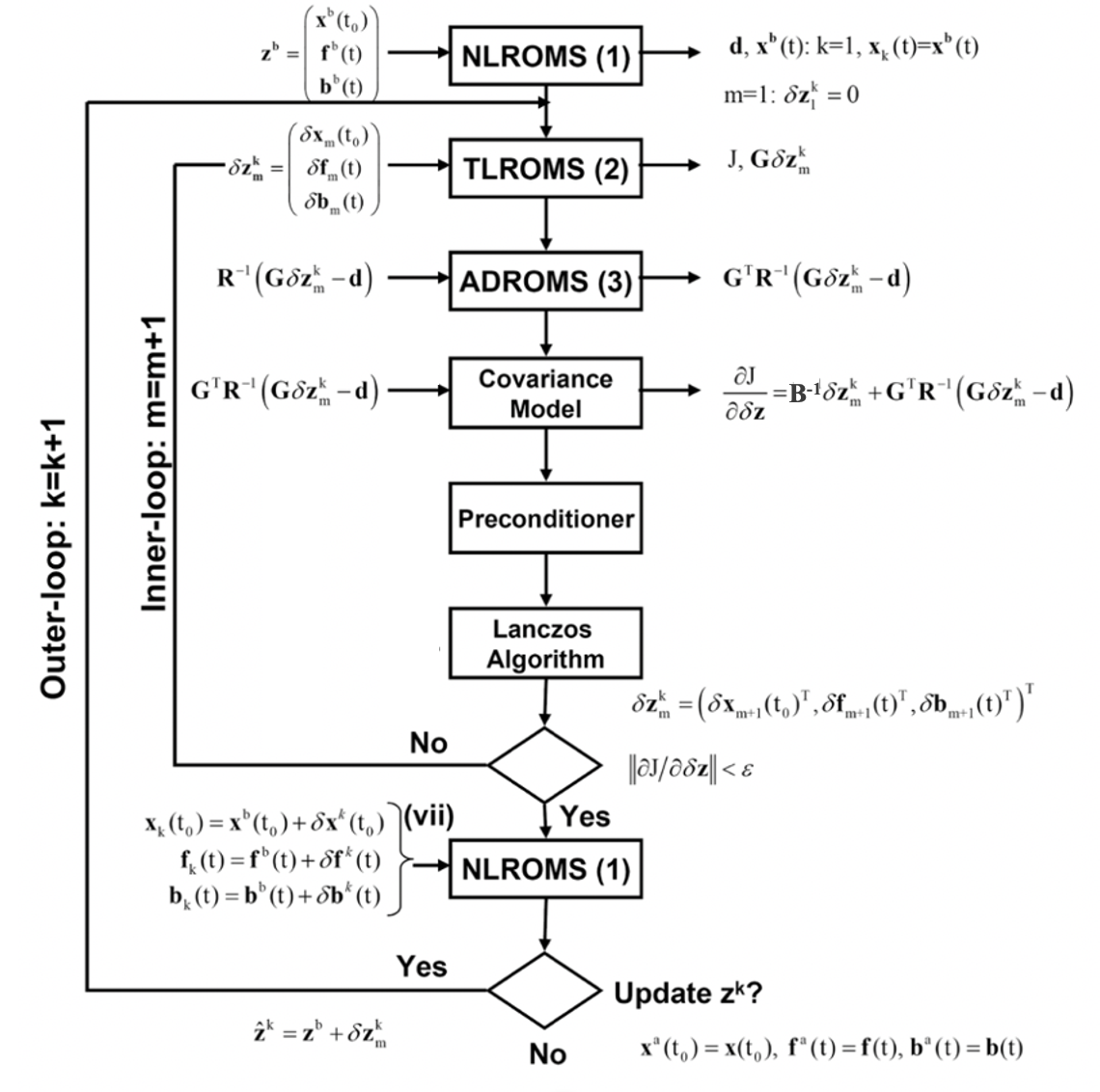
Figure 1: A flow chart illustrating IS4D-Var algorithm.

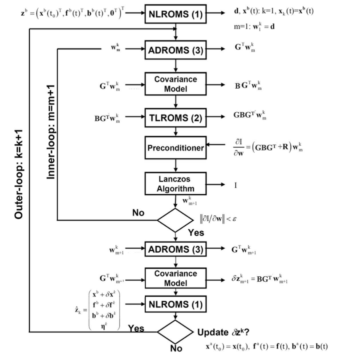
Figure 2: The flow chart illustrating RBL4DVAR algorithm.

Decomposition of spatial domain $\Omega$.
We will consider a 2D decomposition of $\Omega\subseteq\mathbb{R}^{3}$ in x- and y-direction and denote $\Omega_{xy}$ the spatial domain to decompose.

ROMS uses a parallelization approach that partitions domain $\Omega_{xy}$ into tiles (see Figure 3) [2]

$$\Omega_{xy}=\bigcup_{i=0}^{N_{sub}-1}tile_{i}$$ (8)

where $N_{sub}=NtileI\times NtileJ$; $NtileI$ and $NtileJ$ are the number of tiles set in the input file in x- and y-direction, respectively.
We denote by $HI$ and $HJ$ the overlapping tiles regions (i.e ghost or halo area in ROMS) in x- and y-direction, respectively.

Decomposition of time interval $\Delta$.
ROMS does not yet implement decomposition in time direction.

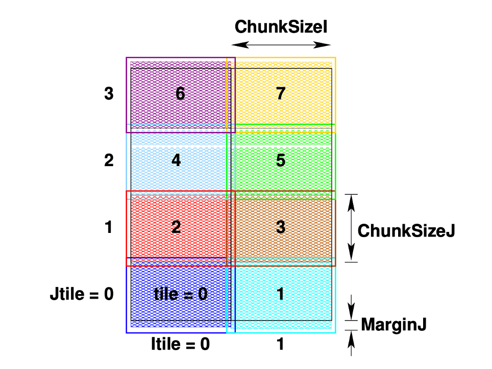
Figure 3: A tiled grid in xy-plane with some internal ROMS parameters.

Ocean model reduction. ROMS allows each tile (or subdomain, see Figure 3) to compute local solutions of TLROMS and ADROMS.
For $i=0,1,\ldots,N_{sub}-1$ and $k=1,\ldots,N_{t}$ local TLROMS on local domain $tile_{i}$ computes

$$\delta x_{i}^{ROMS}(t_{l})\simeq M_{i,(l-1,l)}u_{i}(t_{l-1})$$ (10)

and local ADROMS on local domain $tile_{i}$ computes

$$u_{i}^{*}(t_{l-1})=M_{i,(l-1,l)}^{T}p_{i}(t_{l}),$$ (11)

where $x_{i}$, $u_{i}$, $u_{i}^{*}$, $M_{i}$, $p_{i}$ are the restriction on $tile_{i}$ of variables $x$, $u$, $u^{*}$, $M$ and $p$ and $M_{i,(l-1,l)}$ is discrete model from $t_{l-1}$ to $t_{l}$.
DD-4DVar method introduces model reduction by using the background $x^{b}$ as local initial values. For $n=0,1,\ldots,\bar{n}$ (outer loop of DD–4DVAR method [1]) do: for $k=1,\ldots,N_{t}$, posed $x_{i,k}^{0}\equiv x_{i,k}^{b}$ $\forall i=0,1,\ldots,N_{sub}-1$, we let $x_{i,k}^{{M}_{i,k}}$ be the solution of the local model

$$(P_{i,k}^{{M}_{i,k},n})_{i=0,1\ldots,N_{sub}-1,r=1,\ldots,N_{t}}\ :\quad\left\{\begin{array}[]{ll}x_{i,k}^{\mathcal{M}_{i,k},n}=M_{i,k}x_{i,k-1}^{n}+b_{i,k},\\ x_{i,k-1}^{n}=x_{i,k}^{\mathcal{M}_{i,k},n},\\ x_{i,k-1}^{n}/HI=x_{i_{I},k-1}^{n}/HI,\ \ (\ref{co}.1)\\ x_{i,k-1}^{n}/HJ=x_{i_{J},k-1}^{n}/HJ,\ (\ref{co}.2)\end{array}\right.$$ (12)

where $i_{I}=0,\ldots,n_{I}-1$, $i_{J}=0,\ldots,n_{J}-1$, $n_{I}$ and $n_{J}$ are respectively numbers of adjacent tiles in x- and y-direction, $b_{i,r}^{k}$ and $M_{i}^{r}$ are respectively background on $tile_{i}\times\Delta_{r}$, the vector accounting boundary conditions of $tile_{i}$ and the restriction in $tile_{i}$ of the matrix in (1) that is

$$M_{k}\equiv M_{\bar{s}_{r-1},\bar{s}_{r}}:=M_{\bar{s}_{r-1},\bar{s}_{r-1}+1}\cdots M_{\bar{s}_{r}-1,\bar{s}_{r}}.$$ (13)

In the following, we neglect the dependency on outer loop iteration $n$ of DD–4DVAR method. We underline that local TLROMS and ADROMS in (6) and (7) are obtained by using MPI exchange for boundary conditions, regardless of local solution on overlap area, namely they do not consider overlapping tiles conditions in (12.1) and (12.2). Consequently, we need to modify local TLROMS and ADROMS in (10) and (11) taking into account of (12.1) and (12.1) conditions. More precisely,

Similarly, we need to modify local ADROMS in (11). More precisely,

Figure 4: A region within the domain

4D-VAR DA Operator Reduction.
Operator reduction involves the inner loop in Figure 1.
ROMS [2] computes and minimizes the operator

$$\mathbf{J}_{tile_{i}}^{ROMS}:=\mathbf{J}^{ROMS}/tile_{i}$$ (18)

where $\mathbf{J}^{ROMS}$ is defined in (2) and $\mathbf{J}^{ROMS}/(tile_{i})$ is the IS4D-Var functional in each tile $tile_{i}$ with MPI exchange of boundary conditions, $\forall i=0,1,...,N_{sub}-1$.

Local 4D–VAR DA functional in [1] is defined as follows

$$\mathbf{J}_{tile_{i}\times\Delta_{r}}^{DD-4DVar}:=\mathbf{J}_{i,k}(x_{i,k})=\mathbf{J}(x_{i,k})/(tile_{i}\times\Delta_{k})+\mathcal{O}_{IJ}(x_{i,k})$$ (19)

where

$$\mathbf{J}(x)=\alpha\|x-x^{b}\|_{\textbf{B}^{-1}}^{2}+\|Gx-y\|_{\textbf{R}^{-1}}^{2},$$ (20)

is the DD-4DVar functional in [1],

$$\mathcal{O}_{IJ}(x_{i,k})=\sum_{i_{I}=1}^{n_{I}}\beta_{i_{I},k}\cdot\|x_{i,k}/HI-x_{i_{I},k}/HI\|_{\textbf{B}_{i_{I}}^{-1}}^{2}+\sum_{i_{J}=1}^{n_{J}}\beta_{i_{J},k}\cdot\|x_{i,k}/HJ-x_{i_{J},k}/HJ\|_{\textbf{B}_{i_{j}}^{-1}}^{2}$$ (21)

is the overlapping operator on overlapping tiles region $HI$ and $HJ$, and

$$\mathbf{J}_{i,k}(x_{i,k})/(tile_{i}\times\Delta_{k})=\alpha_{i,k}\cdot\|x_{i,k}-x_{i,k}^{{M}_{i,k}}\|_{\textbf{B}_{i}^{-1}}+\|{G}_{i,r}x_{i,k}-y_{i,k}\|_{\textbf{R}_{i}^{-1}}^{2}$$ (22)

is the restriction of $\mathbf{J}$ on $tile_{i}\times\Delta_{k}$, where $x^{b}$ is background, $y$ is observations vector in $\Delta$, $y_{i,k}$ is observations vector in $\Delta_{k}$; $\mathbf{B}_{i}$, $\mathbf{B}_{i_{I}}$, $\mathbf{B}_{i_{J}}$ are respectively the restrictions of covariance matrix $\mathbf{B}$ to $tile_{i}$, $HI$ and $HJ$; $G_{i,r}$, $\mathbf{R}_{i}$ are restriction of matrices $G$ and $\mathbf{R}$ to $tile_{i}$ in $\Delta_{k}$. Parameters $\alpha_{i,r}$, $\beta_{i_{I}}$ and $\beta_{i_{J}}$ in (21) denotes regularization parameters. We let $\alpha_{i,k}=\beta_{i_{I},k}=\beta_{i_{J},k}=1$, $\forall i_{I}=1,\ldots,n_{I}$ and $\forall i_{J}=1,\ldots,n_{J}$.
Incremental formulation of local 4D–VAR DA functional in (19) is

$${J}_{i,k}(\delta z_{i,k})={J}(\delta z_{k})/(tile_{i}\times\Delta_{k})+\mathcal{O}_{IJ}(\delta z_{i,k})$$

where $\delta z_{i,k}$ are the control variable increments in $tile_{i}\times\Delta_{k}$.

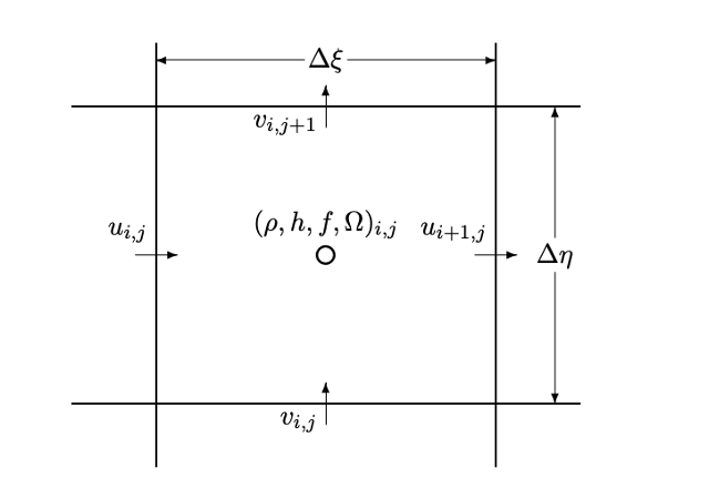
Figure 5: Placement of variables on an Arakawa C grid.

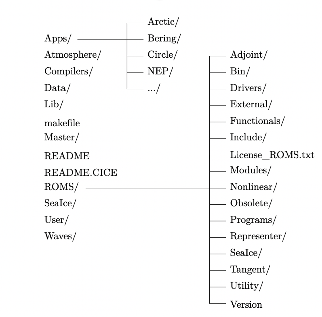
Figure 6: ROMS directory structure.

2.2 DD-4DVarDA in ROMS code

In Figure 6 the ROMS directory structure is shown. We focus on ROMS folder, in particular, on its folders: Tangent and Adjoint.

1. ROMS.
   We need to modify routines in ROMS folder implementing decomposition as in (9) (see step 1).
   Decomposition of time interval involves modification of initial conditions of nonlinear model, in TLROMS and ADROMS.
   Routines involving initialization are (see Figure 6):

   1. initial routine in Nonlinear folder: initializes all model variables (it is called in main3d).

   2. tl_initial routine in Tangent folder: initializes all tangent model variables (it is called in i4dvar).

   3. ad_initial routine in Adjoint folder: initializes all adjoint model variables(it is called in i4dvar).

   Main actions to apply DD in time in ROMS are described below.

2. TLROMS.
   We need to modify TLROMS as in (14) (see step 2), namely we need to compute the overlapping vector in (15) and (16) and add them to tangent variables.
   

   We note that primitive equations of motion [5] are written in flux form transformed using orthogonal curvilinear coordinates ($\xi,\eta$) (see Figure 5).
   We consider tl_main3d routine. In tangent folder (see Figure 6) this routine is the main driver of TLROMS configurated as a full 3D baroclinic ocean model.
   tl_main3d routine calls the following subrountines.

   1. tl_set_massflux calls tl_set_massflux_tile.
      tl_set_massflux_tile: computes “in situ” tangent linear horizontal mass flux.

   2. tl_rho_eos calls tl_rho_eos_tile.
      tl_rho_eos_tile: computes “in situ” the density and other quantities (temperature, salinity,…).
      

   3. tl_omega: computes vertical velocity (no modifications because DD is only horizontal, there are not overlap region along vertical direction).

3. ADROMS.
   Similarly to TLROMS, we need to modify ADROMS as in (17) (see step 3), namely we need to compute and add the overlapping vector in (15) and (16) to adjoint variables.
   We consider ad_main3d routine. In Adjoint folder (see Figure 6) this routine is the main driver of ADROMS configurated as a full 3D baroclinic ocean model.
   ad_main3d routine calls the following subrountines.

   1. ad_rho_eos: computes “in situ” density and other associated quantities.
      

   2. ad_set_mass_flux: compute “in situ” adjoint horizontal mass fluxes.
      

   3. ad_set_avg: accumulates and computes output time-averaged adjoint fields. (probably no modifications are needed).

4. IS4D-Var.
   We need to modify routines in ROMS folder as in (23) (see step 4).
   

3 ROMS test cases

We have installed ROMS on the high-performance hybrid computing architecture of the Sistema Cooperativo Per Elaborazioni scientifiche multidiscipliari data center, located in the University of Naples Federico II. More precisely, the HPC architecture is made of 8 nodes, consisting of distributed memory DELL M600 blades connected by a 10 Gigabit Ethernet technology. Each blade consists of 2 Intel Xeon@2.33 GHz quadcore processors sharing 16 GB RAM memory for a total of 8 cores/blade and of 64 cores, in total.
We consider test cases referred to IS4D-Var and RBL4DVAR configured for the U.S. west coast and the California Current System (CCS). This configuration, referred to as WC13, has 30 km horizontal resolution, and 30 levels in the vertical and data assimilated every 7 days during the period July 2002 – Dec. 2004.

• IS4DVAR test cases.
  

  To run this application I need to take the following steps.

  • I customize build_roms.csh script in IS4DVAR folder and define the path to the directories where all project’s files are kept.

    • I set USE_MY_LIBS to yes, then I modify source code root file Complilers/my_build_paths.sh and edit the appropriate paths for the desired compiler.

  • I customize the ROMS input file (roms_wc13_2hours.in/roms_wc13_daily.in) and specify the appropriate values of tile numbers in the I-direction and J-direction i.e. NtileI=2 and NtileJ=4 (see Figure 3).

  • I modify ARmake.inc in Lib folder to create the libraries for serial and parallel ARPACK.

  • I customize Linux-ifort.mk (Fortran compiler is ifort) and define library locations.

  • I create PBS scripts to run the test cases.

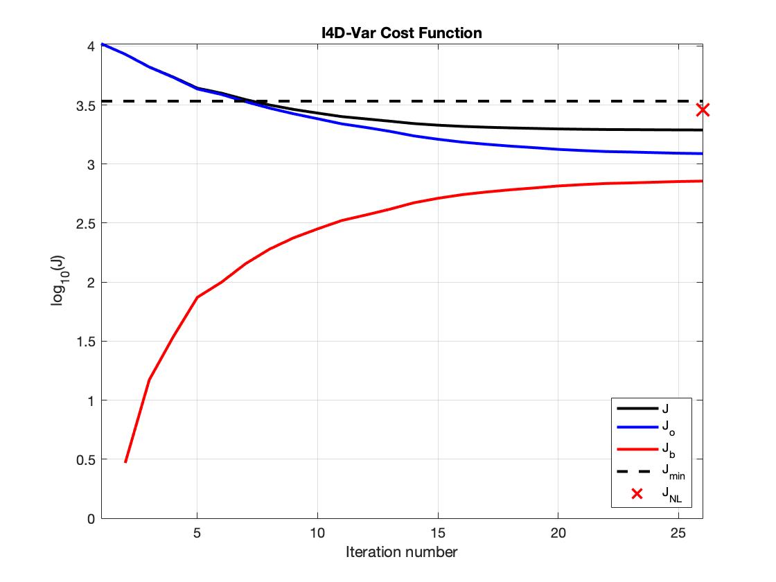
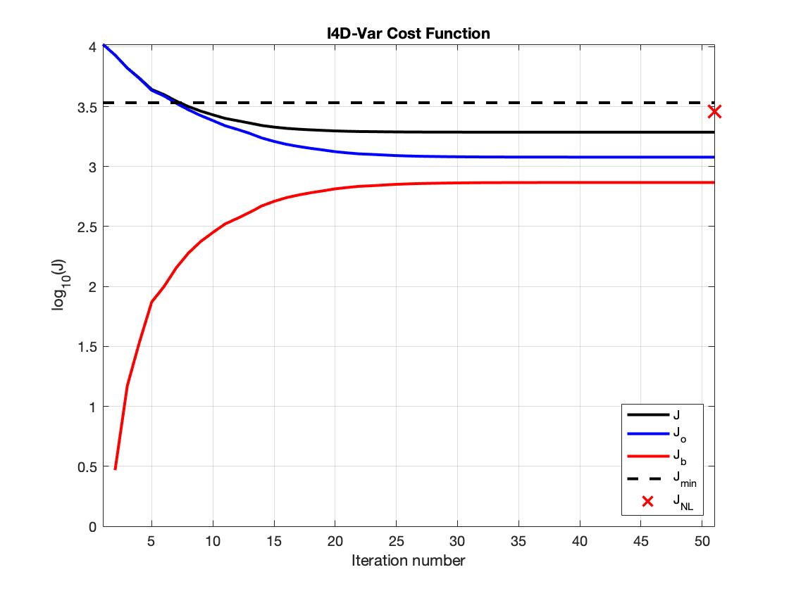
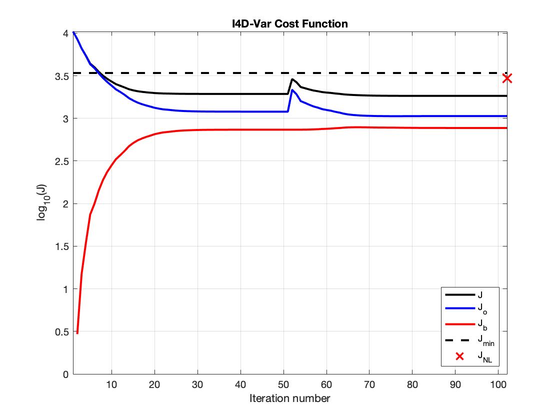
Figure 7: IS4D-Var Cost Function: case1, case2, case3 and case 4, respectively, using roms_wc13_2hours.in input file.

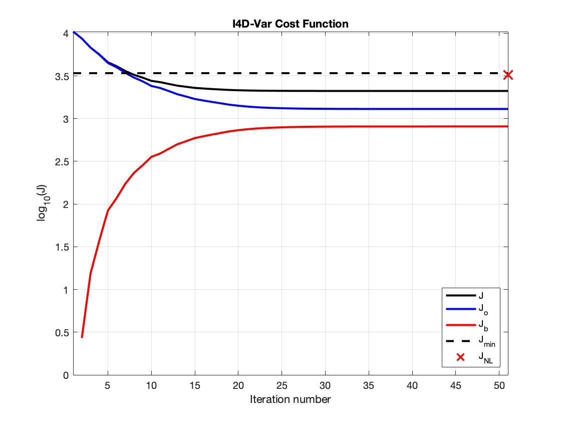
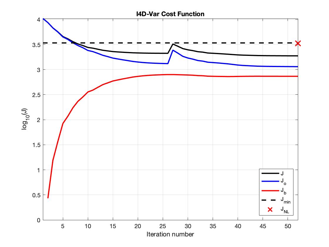
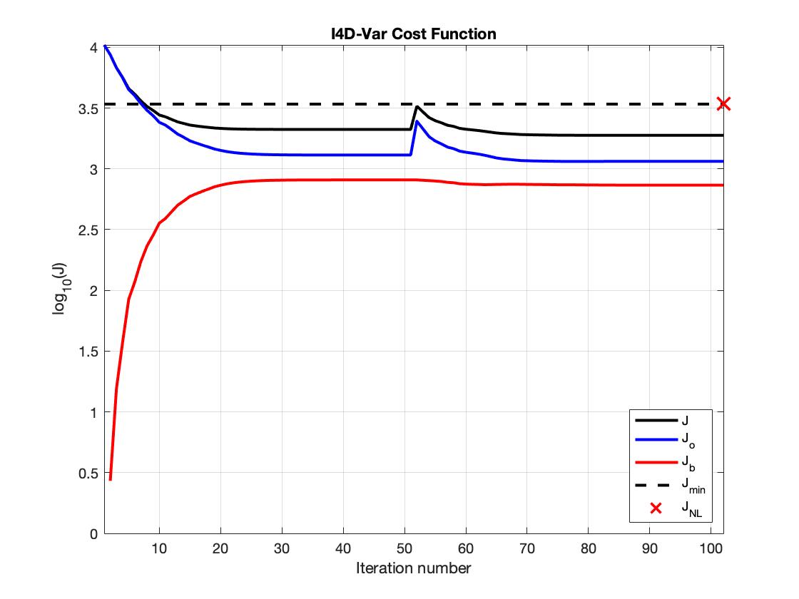
Figure 8: IS4D-Var Cost Function: case1, case2, case3 and case 4, respectively, using roms_wc13_daily.in input file.

  Figures 8 and 7 show results obtained applying DD in space by considering $NtileI\times NtileJ$ tiles and input files roms_wc13_2hours.in and roms_wc13_daily.in, respectively. They show total cost function $J$ (black curve), observation cost function $Jo$ (blue curve), and background cost function $Jb$ (red curve) and the theoretical minimum value $J_{min}=n_{obs}/2$ (dashed black line) plotted on a $log_{10}$ scale. We observe that the solution has more or less converged by 25 iterations.
  We will refer to the following quantities: Nouter number of outer loops, Ninner inner loop, $T_{Casei}^{node}$ elapsed time for each node in seconds, $T_{max}$ and $T_{min}$ maximum and minimum elapsed time among nodes in seconds.
  We consider:

  • case 1: Nouter=1 and Ninner=25;

  • case 2: Nouter=1 and Ninner=50;

  • case 3: Nouter=2 and Ninner=25;

  • case 4: Nouter=2 and Ninner=50;

  In Tables 1, 2 and 3, 4 we report elapsed time for each process considering roms_wc13_2hours and roms_wc13_daily.in input file, respectively.
  

  $Node$	$T_{Case1}^{node}$	$T_{Case2}^{node}$	$T_{Case3}^{node}$	$T_{Case4}^{node}$
  $0$	$1.56\times 10^{3}$	$3.24\times 10^{3}$	$3.124\times 10^{3}$	$6.42\times 10^{3}$
  $1$	$1.58\times 10^{3}$	$3.29\times 10^{3}$	$3.17\times 10^{3}$	$6.49\times 10^{3}$
  $2$	$1.58\times 10^{3}$	$3.29\times 10^{3}$	$3.17\times 10^{3}$	$6.50\times 10^{3}$
  $3$	$1.58\times 10^{3}$	$3.28\times 10^{3}$	$3.16\times 10^{3}$	$6.50\times 10^{3}$
  $4$	$1.58\times 10^{3}$	$3.29\times 10^{3}$	$3.17\times 10^{3}$	$6.50\times 10^{3}$
  $5$	$1.58\times 10^{3}$	$3.29\times 10^{3}$	$3.16\times 10^{3}$	$6.50\times 10^{3}$
  $6$	$1.58\times 10^{3}$	$3.29\times 10^{3}$	$3.16\times 10^{3}$	$6.50\times 10^{3}$
  $7$	$1.58\times 10^{3}$	$3.28\times 10^{3}$	$3.17\times 10^{3}$	$6.49\times 10^{3}$

  Table 1: Elapsed time in seconds for each process related to roms_wc13_2hours input file.

  	$T_{max}$	$T_{min}$
  ${Case1}$	$1.58\times 10^{3}$	$1.56\times 10^{3}$
  $Case2$	$3.29\times 10^{3}$	$3.24\times 10^{3}$
  ${Case3}$	$3.17\times 10^{3}$	$3.12\times 10^{3}$
  ${Case4}$	$6.50\times 10^{3}$	$6.42\times 10^{3}$

  Table 2: Maximum and minimum elapsed time in seconds among nodes related to roms_wc13_2hours.in input file.

  $Node$	$T_{Case1}^{node}$	$T_{Case2}^{node}$	$T_{Case3}^{node}$	$T_{Case4}^{node}$
  $0$	$1.41\times 10^{3}$	$2.95\times 10^{3}$	$2.79\times 10^{3}$	$5.97\times 10^{3}$
  $1$	$1.41\times 10^{3}$	$2.96\times 10^{3}$	$2.83\times 10^{3}$	$5.99\times 10^{3}$
  $2$	$1.41\times 10^{3}$	$2.97\times 10^{3}$	$2.82\times 10^{3}$	$5.99\times 10^{3}$
  $3$	$1.41\times 10^{3}$	$2.97\times 10^{3}$	$2.82\times 10^{3}$	$6.00\times 10^{3}$
  $4$	$1.41\times 10^{3}$	$2.97\times 10^{3}$	$2.82\times 10^{3}$	$5.98\times 10^{3}$
  $5$	$1.41\times 10^{3}$	$2.96\times 10^{3}$	$2.82\times 10^{3}$	$5.99\times 10^{3}$
  $6$	$1.41\times 10^{3}$	$2.96\times 10^{3}$	$2.82\times 10^{3}$	$6.00\times 10^{3}$
  $7$	$1.41\times 10^{3}$	$3.00\times 10^{3}$	$2.82\times 10^{3}$	$6.00\times 10^{3}$

  Table 3: Elapsed time in seconds for each process releted to roms_wc13_daily.in input file.

  	$T_{max}$	$T_{min}$
  ${Case1}$	$1.41\times 10^{3}$	$1.41\times 10^{3}$
  $Case2$	$3.00\times 10^{3}$	$2.95\times 10^{3}$
  ${Case3}$	$2.83\times 10^{3}$	$2.79\times 10^{3}$
  ${Case4}$	$5.97\times 10^{3}$	$5.97\times 10^{3}$

  Table 4: Maximum and minimum elapsed time in seconds among nodes related to roms_wc13_daily.in input file.

• RBL4DVAR.
  

  To run this application I need to take the following steps.

  • I customize build_roms.csh scripts in RBL4DVAR folders and define the path to the directories where all project’s files are kept.

  • I customize the ROMS input file (roms_wc13_2hours.in/roms_wc13_daily.in) and specify the appropriate values of tile numbers in the I-direction and J-direction i.e. NtileI=2 and NtileJ=4 (see Figure 3).

  • I create a PBS script to run the test cases.

• IS4D-Var vs RBL4DVAR.
  

  IS4D-Var and RBL4DVAR algorithms are based on a search for the best circulation estimate in the space spanned by the model control vector and in the dual space spanned by the observations, respectively. We note that ${n_{obs}}<<N_{p}$, where ${n_{obs}}$ is number of observations and $N_{p}$ is dimension of model control vector. Hence, the dimension of observation space is significantly smaller than the model control space, the dual formulation can reduce both memory usage and computational cost. Consequently, it appears that the dual formulation should be an easier problem to solve because of the considerably smaller dimension of the space involved, but it has practical barriers to convergence.
  Consequently, we consider three applications of dual formulation:

  1. using the standard $R^{-1/2}$ preconditioning with a conjugate gradient (RBL4DVAR) method;

  2. using the $R^{-1/2}$ preconditioning and minimum residual algorithm (MINRES);

  3. using a restricted B-preconditioned conjugate gradient (RPCG) approach.

  Figure 9 and 10 shows the convergence of minimization algorithms RBL4DVAR and RBL4DVAR, MINRES, and RPCG compared to primal formulation IS4DVAR by considering $Nouter=1$, $Ninner=50$ and $Nouter=1$, $Ninner=25$. We observe that the performance of RPCG is superior to both MINRES and RBL4DVAR, in particular, PCG ensures that RPCG converges at same rate as IS4D-Var.

• Observation impact and observation sensitivity.
  The observations assimilated into the model are:

  • SST satellite: Sea Surface Temperature;

  • SSH satellite: Sea Surface Heights;

  • Argo floats: hydrographic observations of temperature and salinity.

  We consider the time average transport across 37N over the upper 500 m, denoted by $I_{37N}$, and given by

  $$I_{37N}(x)=\frac{1}{N}\sum_{i=1}^{N}h^{T}x_{i}$$ (24)

  where $h$ is a vector with non-zero elements corresponding to the velocity grid points that contribute to the transport normal to the 37N section shown in Figure 12, $N$ is the number of time steps during the assimilation interval, $x_{i}$ is the model state-vector at time $i\Delta t$, and $\Delta t$ is the model time step. We consider scalar functions of ocean state vector $I=I(x)$, prior $I^{b}=I(x^{b})$ and posterior ocean state vector $I^{a}=I(x^{a})$, where $x^{b}$ is background circulation estimate and $x^{a}$ is 4D-Var analysis. The circulation analysis increment $\delta x^{a}(t)$ at instant time $t$ in interval time $[t_{0},t_{0}+7]$ of each 4D-Var cycle is given

  $$\delta x^{ROMS}(t)=x^{a}(t)-x^{b}(t),$$ (25)

  consequently, transport increment $\Delta I$ during each assimilation cycle can be expressed as:

  $$\Delta I=I^{a}-I^{b}=I(x^{b}+\delta x)-I^{b}\simeq\delta x^{T}(\partial J/\partial x),$$ (26)

  using the tangent linear assumption in (6), (5) and (4), the circulation analysis increment is given by

  $$\delta x^{ROMS}(t)=M(t,t_{0})\tilde{\mathbf{K}}d,$$ (27)

  where $M(t,t_{0})$ represents the perturbation tangent linear model for the time interval $[t_{0},t]$, $\tilde{\mathbf{K}}$ is an approximation of $\mathbf{K}$ defined in (5) and $\mathbf{d}$ is innovation vector. Then, increment defined in (26) become

  $$\Delta I\simeq d^{T}\tilde{K}^{T}M^{T}(\partial I/\partial x),$$ (28)

  where $\tilde{K}$ represents adjoint of Kalman gain matrix.
  Consequently, 37N time increment of averaged transport in (24) is:

  $$\Delta I_{37N}\simeq\frac{1}{N}d^{T}\tilde{K}^{T}\sum_{l=1}^{N}(M_{l})^{T}h=d^{T}g=d^{T}(g^{x}+g^{f}+g^{b})$$ (29)

  or

  $$\Delta I_{37N}\simeq\sum_{l=1}^{n_{obs}}(y_{l}-H_{l}(x^{b}(t)))g_{l},$$ (30)

  namely, each observation contributes to the calculation of the increase, where $g\simeq\frac{1}{N}\tilde{K}\sum_{l=1}^{N}(M_{l})^{T}h$, $g^{x}$ contribution from initial condition increment, $g^{f}$ contribution from surface forcing increment, $g^{b}$ contribution from open boundary increment and $M_{l}\equiv M(t_{0},t_{0}+l\Delta t)$.
  Moreover, we consider the sensitivity of $I$ to variations $\delta y_{0}$ in the observations, in particular, we consider $\delta y_{0}=d$.

  Figure 10 shows the total number of observations from each observing platform that were assimilated into the model during cycle, increments and contribution of observations from each platform to

  • NL: nonlinear model;

  • TL: total impact;

  • IC: initial condition;

  • FC: surface forcing conditions;

  • BC: open boundary conditions.

  Figure 13 shows curve represents the evolution of the ocean state vector $I$ in time based on the either the prior or posterior control vector. In the case of the observation impact, the actual contribution of each observation, $y^{o}_{i}$, to the change $\Delta I$ defined in (28) (blue curve vs. black curve) due to data assimilation is revealed. Conversely, the observation sensitivity quantifies the change $\Delta I$ that will occur in $I$ a (red curve vs. blue curve) as a result of perturbations in the observations, $\delta y=\textbf{d}$. In Figures 15, 16 and 17 we show the results obtained by running related tests on SCoPE.

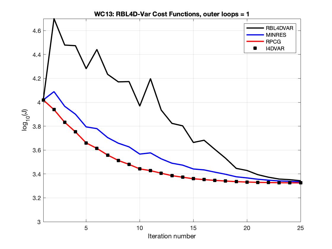
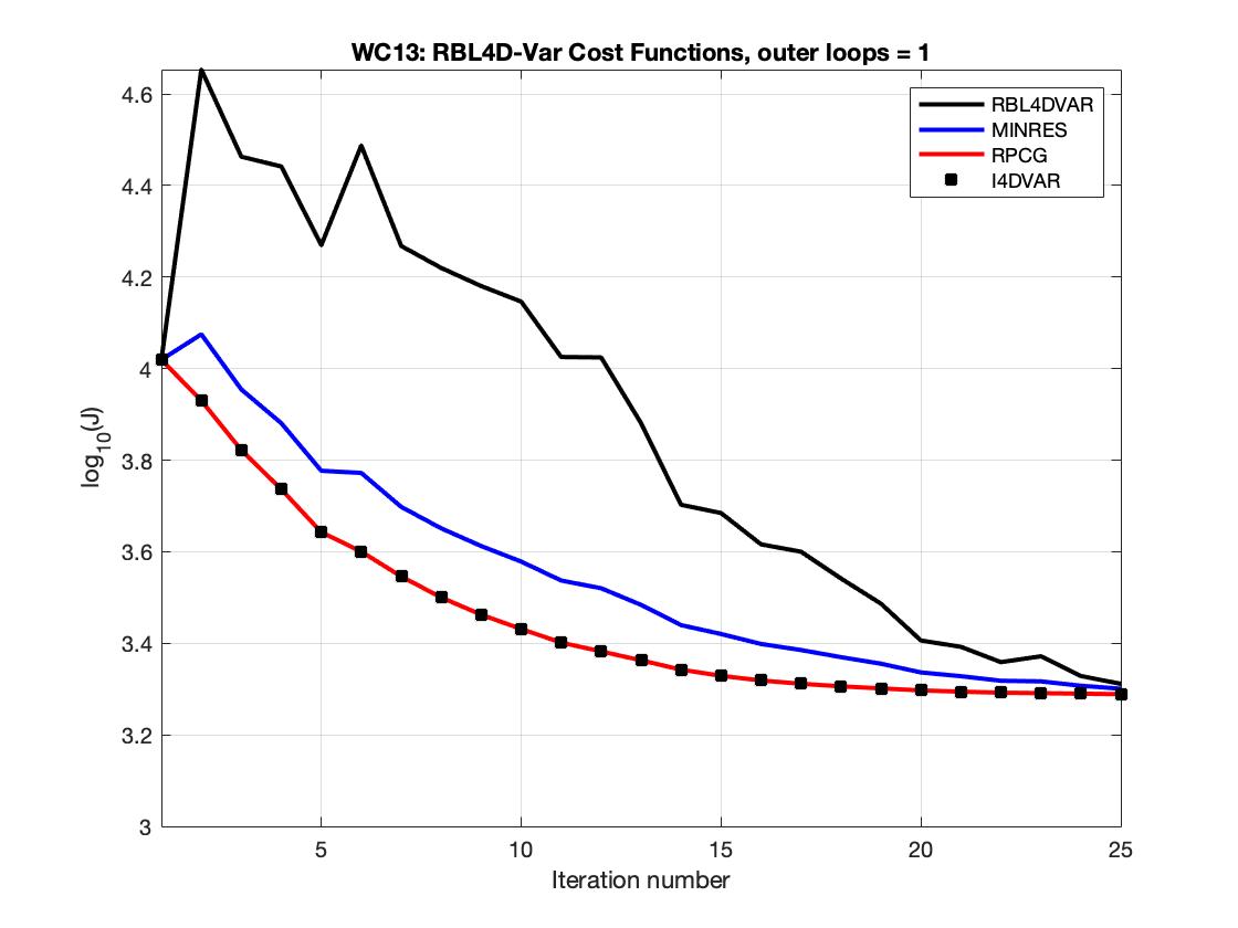
Figure 9: RBL4D-Var Cost functions using roms_wc13 3_2hours.in (left) and roms_wc13_daily.in (right) file input, $Nouter=1$ and $Ninner=25$.

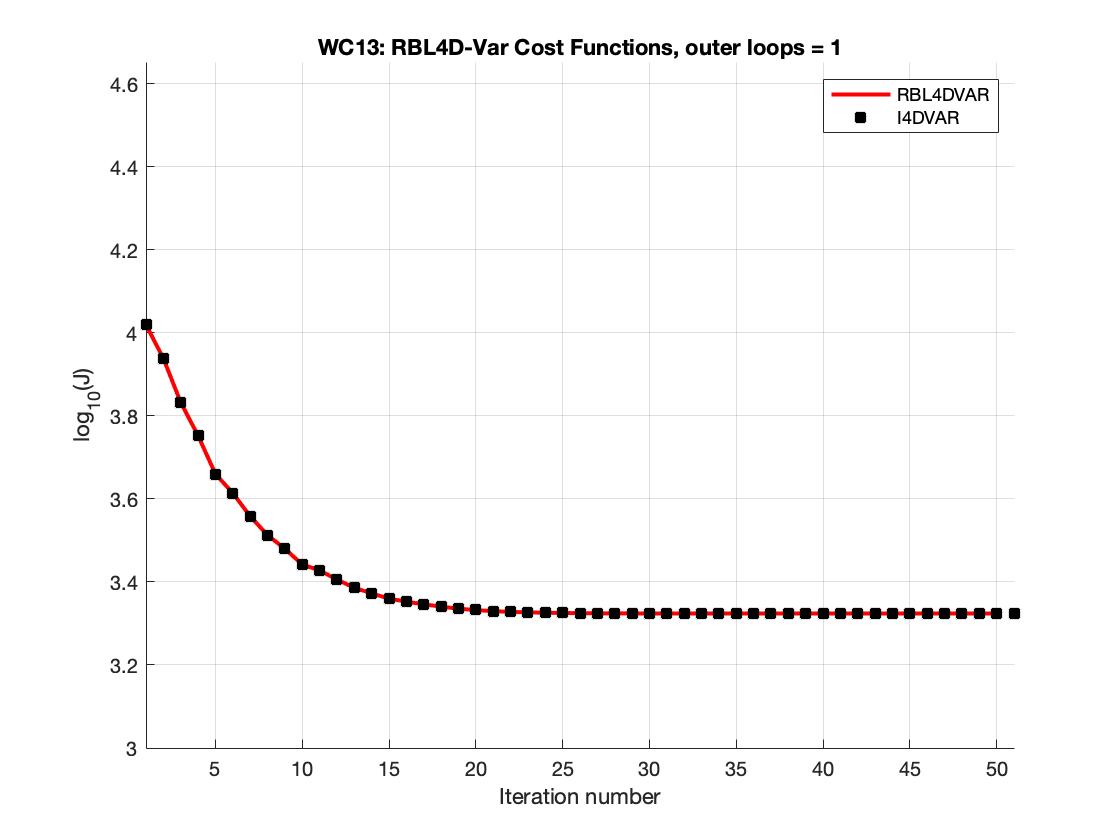
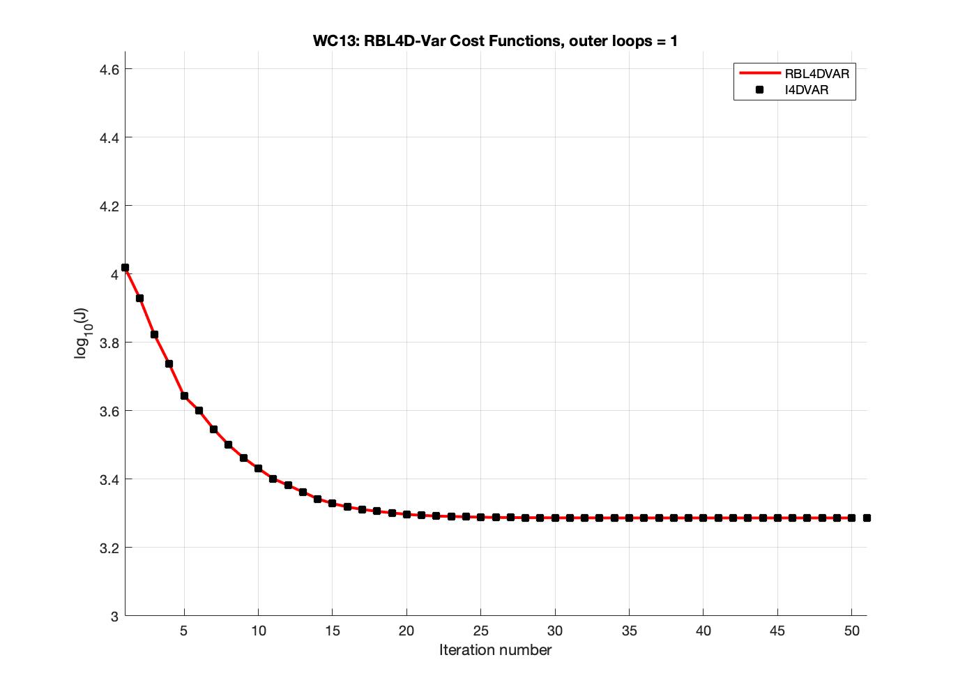
Figure 10: RBL4D-Var Cost functions using roms_wc13 3_2hours.in (left) and roms_wc13_daily.in (right) file input, $Nouter=1$ and $Ninner=50$.

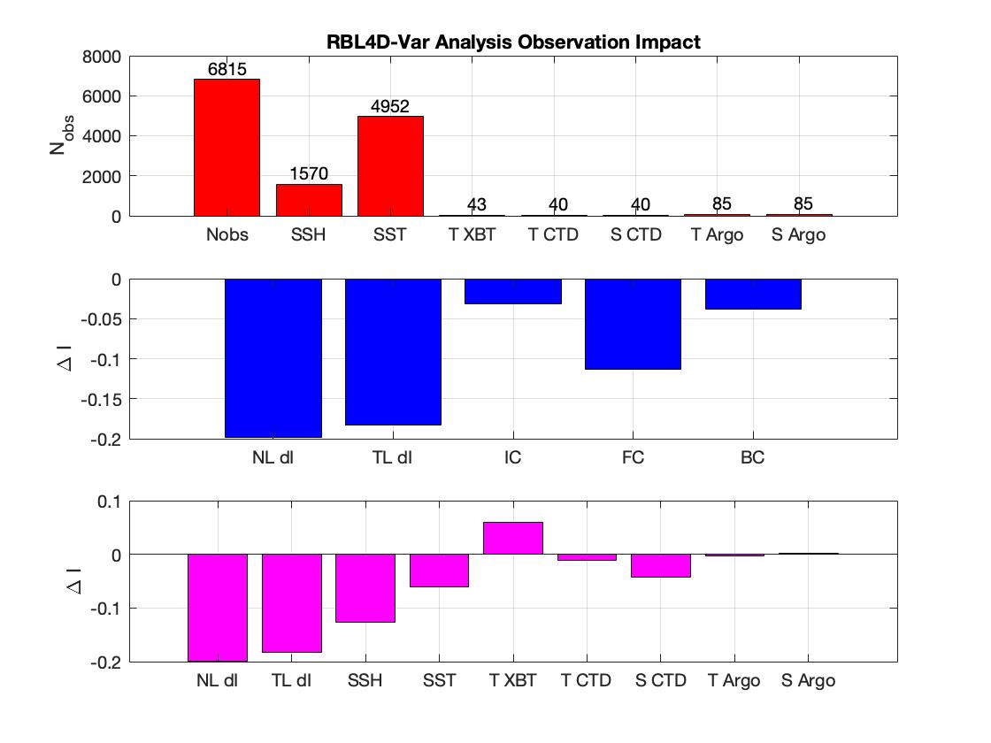
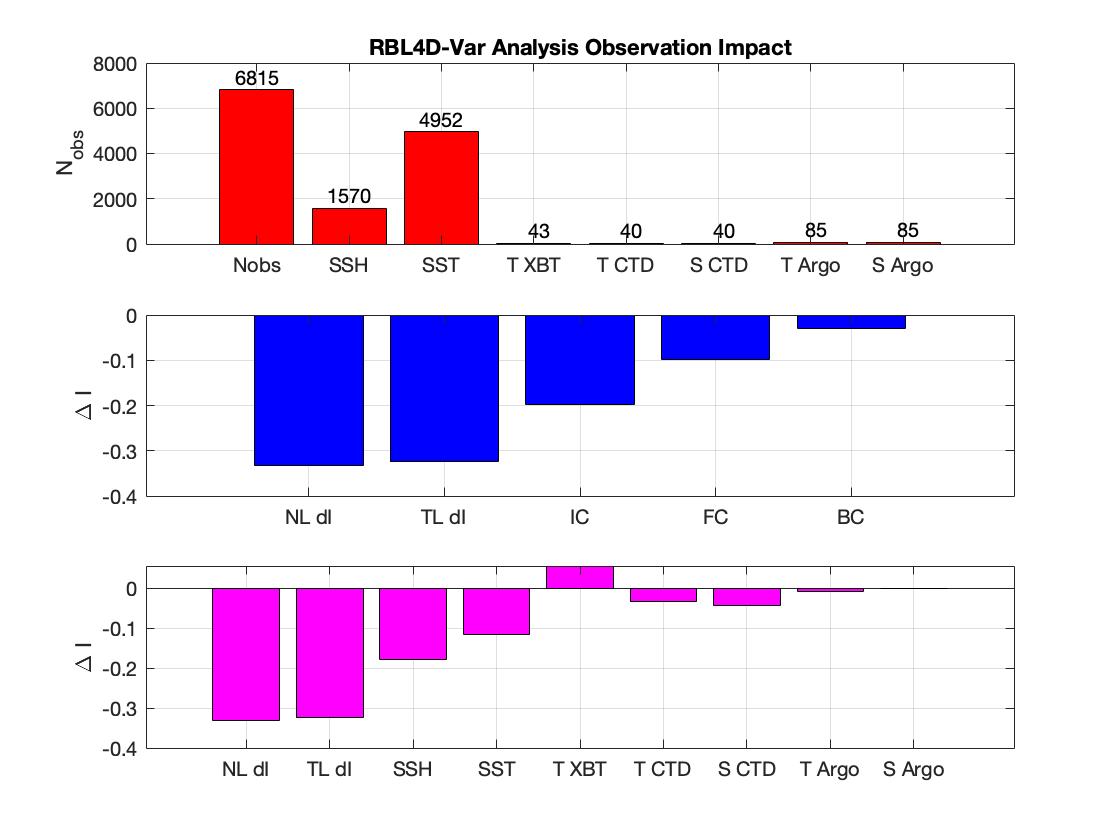
Figure 11: RBL4D-Var observation impact using roms_wc13_2hours.in (left) and roms_wc13_daily.in (right) file.

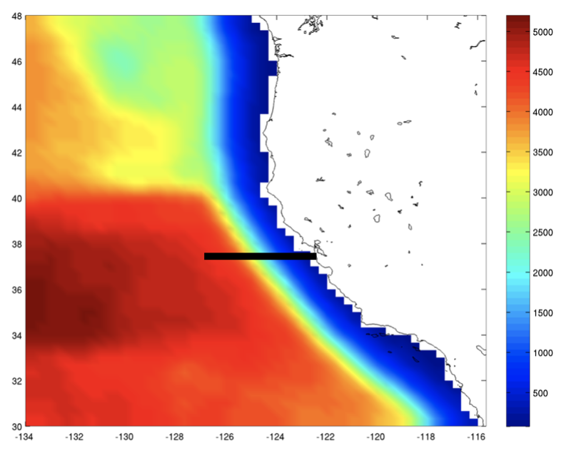
Figure 12: The 37N section along which the time averaged transport is computed from the surface to a depth of 500m.

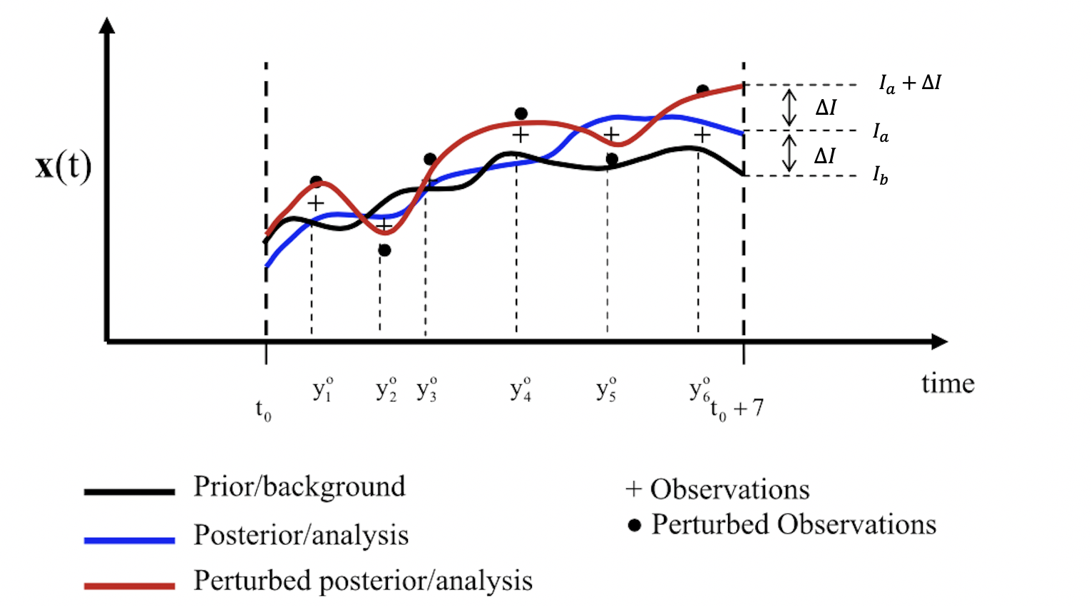
Figure 13: A schematic illustrating difference between the observation impact and observation sensitivity calculations. Fixed time interval $[t_{0},t_{0+7}]$, $y^{o}_{i}$ are observations at various times that it are shown as pluses (+) while perturbed observations, $y^{o}_{i}+\delta y^{o}_{i}$ are indicated by filled circles ($\bullet$). Consequently, red curve is perturbed analysis and blue curve is 4DVar analysis.

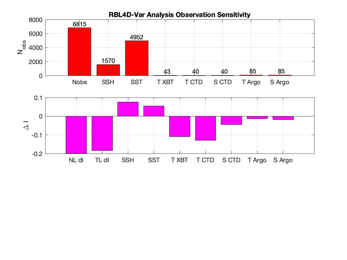
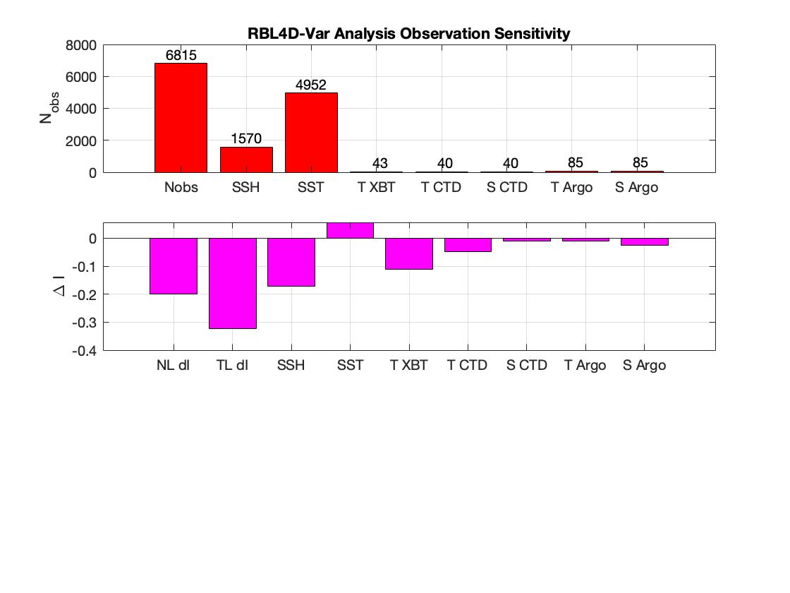
Figure 14: RBL4D-Var observation sensitivity using roms_wc13_2hours.in (left) and roms_wc13_daily.in (right) file.

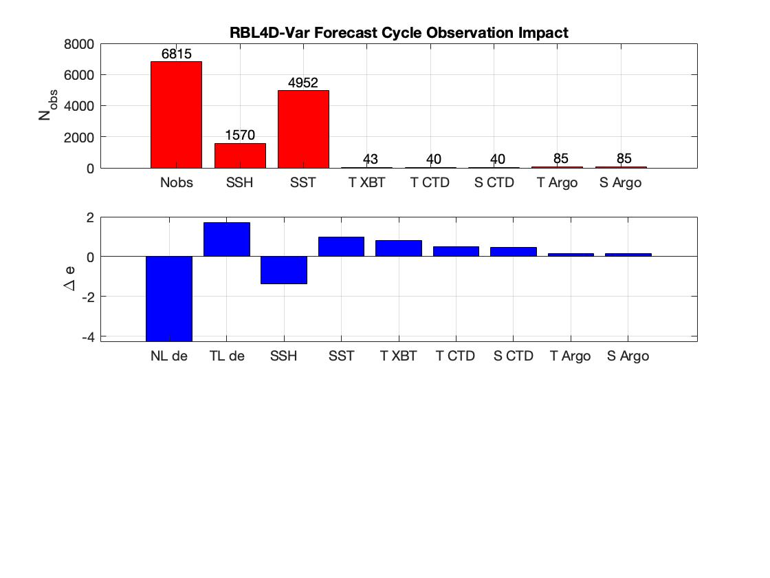
Figure 15: RBL4D-Var forecast impact using roms_wc13_2hours.in (left) and roms_wc13_daily.in (right) file.

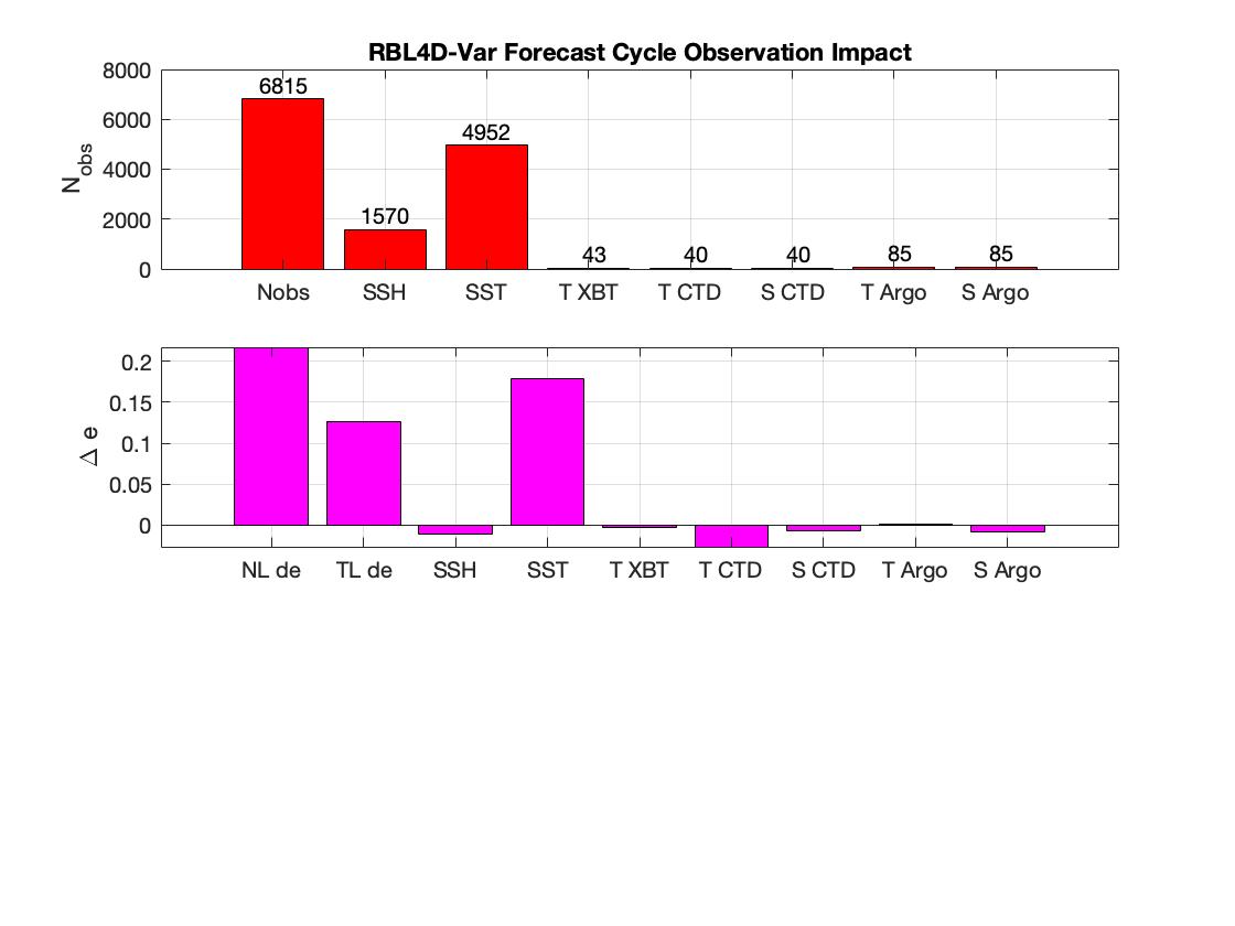
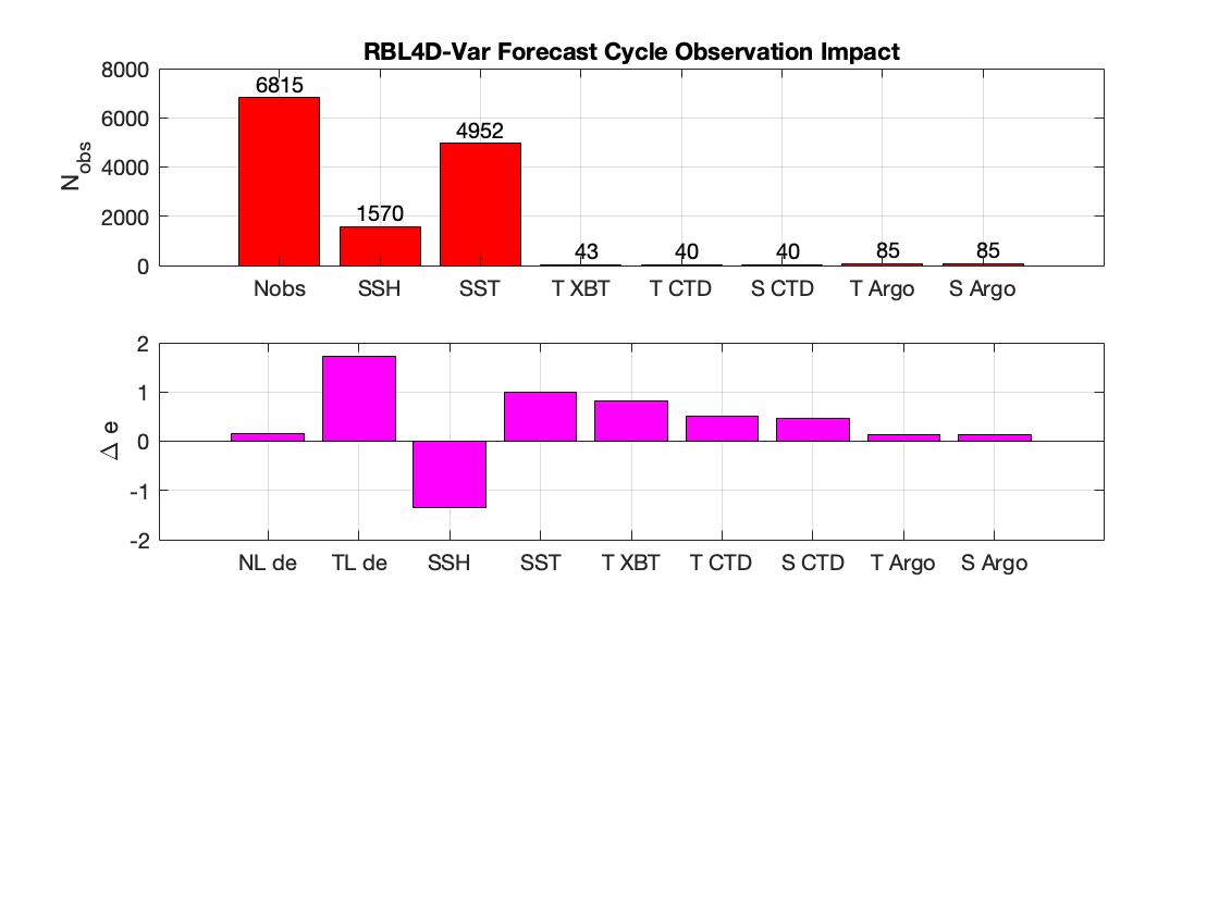
Figure 16: RBL4D-Var forecast impact in observations space using roms_wc13_2hours.in (left) and roms_wc13_daily.in (right) file.

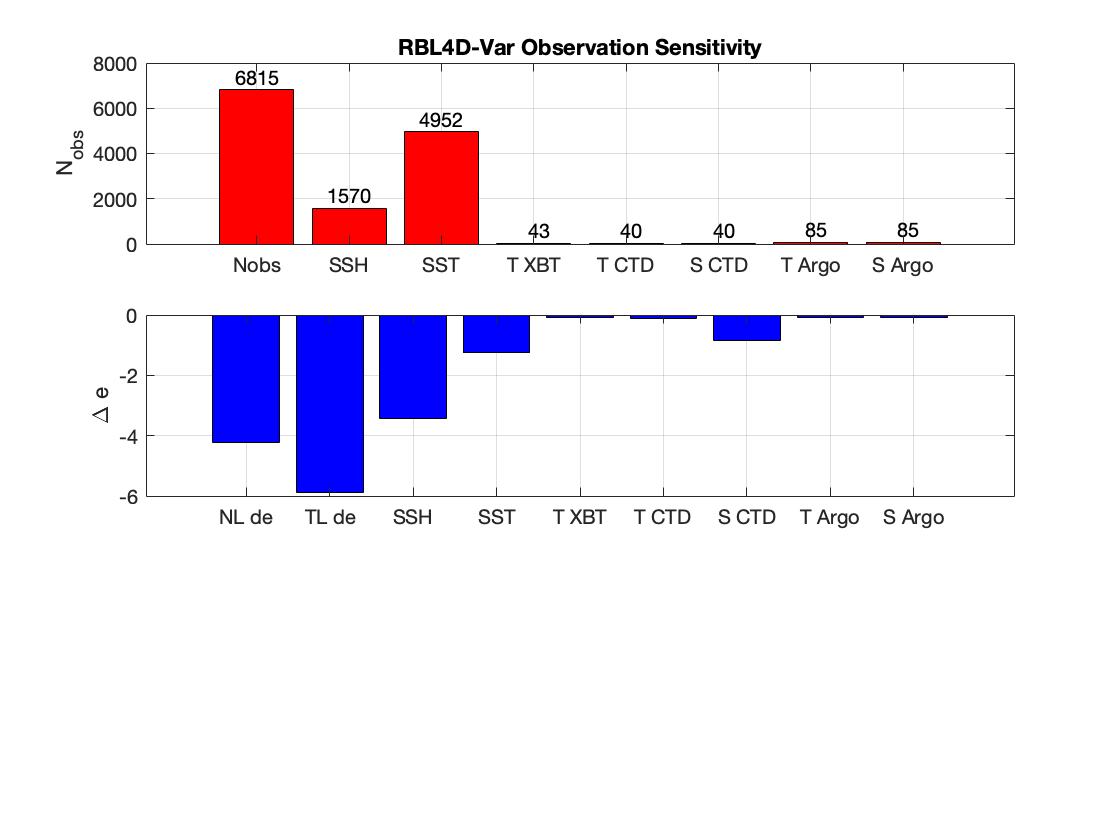
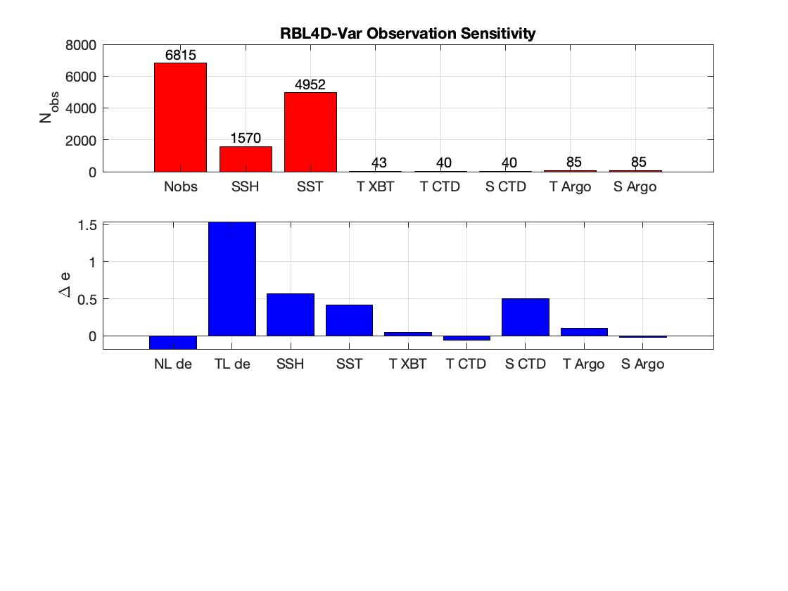
Figure 17: RBL4D-Var forecast sensitivity using roms_wc13_2hours.in (left) and roms_wc13_daily.in (right) file.

4 Future developments

Main modification to apply DD in time in ROMS is described by point (c) in Action 1.1, i.e. introduction of MPI communications in time. More precisely, we need to introduce and manage the MPI communication in space and time. The introduction of DD in time involves the following communications among processes:

• Intra communications: by splitting MPI communicator (OCN_COMM_WORLD) to create local communicators (TASK_COMM_WORLD) to allow communications among processes related to same spatial subdomain but different time intervals.
  MPI commands are

  • MPI_Comm_split: partitions the group of MPI processes into disjoint subgroups and creates a new communicator (TASK_COMM_WORLD) for each subgroup.

  • MPI_Isend and MPI_Irecv: sends and receives initial conditions by setting the new communicator obtained from MPI_Comm_split.

• Inter communications: by creating new communicators (OCNi_COMM_WORLD) to allow communications among processes related to different spatial subdomains but same time interval.
  MPI commands are

  • MPI_Intercomm_create: creates an intercommunicator for each subgroup.

  • MPI_Isend and MPI_Irecv: sends and receives boundary conditions by setting the new communicator obtained from MPI_Intercomm_create.

References

- [1] D’Amore, L., Cacciapuoti, R., 2021: “Model Reduction in Space and Time for decomposing ab initio 4D Variational Data Assimilation Problems”, Applied Numerical Mathematics, 2021, Volume 160, pp. 242-264 Elsevier, https://doi.org/10.1016/j.apnum.2020.10.003.
- [2] https://www.myroms.org
- [3] Moore, A.M., H.G. Arango, G. Broquet, B.S. Powell, A.T. Weaver, and J. Zavala-Garay, 2011: The Regional Ocean Modeling System (ROMS) 4-dimensional variational data assimilation systems, Part I - System overview and formulation, Progress in Oceanography, 91, 34-49.
- [4] Hedström, K.S., 2018: Technical Manual for a Coupled Sea-Ice/Ocean Circulation Model (Version 5), OCS Study BOEM 2018-007. U.S. Department of the Interior Bureau of Ocean Energy Management Alaska OCS Region. 182 p.
- [5] Arango, H.G., Moore, A.M., Miller, A.J., Cornuelle, B.D., Lorenzo, E.Di, Cornuelle B.D. and Neilson, D.J., 2003: The ROMS Tangent Linear and Adjoint Models: A comprehensive ocean prediction and analysis system.
- [6] D’Amore, L., Arcucci, R., Pistoia, J., Toumi, R. Murli, A. 2017: On the variational data assimilation problem solving and sensitivity analysis, Journal of Computational Physics, pp. 311-326.
- [7] Langland, R. H., and N. Baker, 2004: Estimation of observation impact using the NRL atmospheric variational data assimilation adjoint system. Tellus, 56A, 189–201.
- [8] Gürol, S., Weaver, A. T., Moore, A. M., Piacentini, A., Arango, and H. G., Gratton, S. 2014: B‐preconditioned minimization algorithms for variational data assimilation with the dual formulation. Quarterly Journal of the Royal Meteorological Society, 140(679), 539-556.