Ranking with Confidence for Large Scale Comparison Data

Abstract

In this work, we leverage a generative data model considering comparison noise to develop a fast, precise, and informative ranking algorithm from pairwise comparisons that produces a measure of confidence on each comparison. The problem of ranking a large number of items from noisy and sparse pairwise comparison data arises in diverse applications, like ranking players in online games, document retrieval or ranking human perceptions. Although different algorithms are available, we need fast, large-scale algorithms whose accuracy degrades gracefully when the number of comparisons is too small. Fitting our proposed model entails solving a non-convex optimization problem, which we tightly approximate by a sum of quasi-convex functions and a regularization term. Resorting to an iterative reweighted minimization and the Primal-Dual Hybrid Gradient method, we obtain PD-Rank, achieving a Kendall tau 0.1 higher than all comparing methods, even for 10% of wrong comparisons in simulated data matching our data model, and leading in accuracy if data is generated according to the Bradley-Terry model, in both cases faster by one order of magnitude, in seconds. In real data, PD-Rank requires less computational time to achieve the same Kendall tau than active learning methods.

Keywords Ranking aggregation  $\cdot$ Primal-Dual Hybrid Gradient  $\cdot$ Large scale optimization

1 Introduction

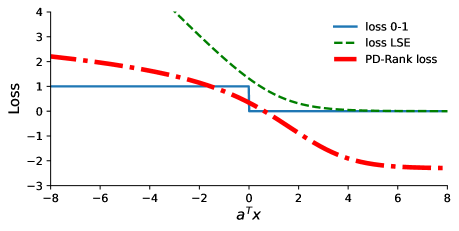
Figure 1: Comparison between 0-1 loss, LSE and PD-Rank loss. On the horizontal axis is the value difference between two items, according to the observed label. If this value is positive, the current ranking respects this label, otherwise, the order is incorrect according to the label. While the 0-1 loss just distinguishes between correct and incorrect ordering, both approximations penalize according to the "degree of correctness". However, we note that for values closer to and less than 0, the proposed PD-Rank loss is a tighter approximation on the 0-1 loss.

If early applications of the ranking problem were focused on voting scenarios [17, 14] and later on ranking of a small set of items where experts consider weighted ratios between pairs of items [33], modern needs call for the rank of a large number of items with noisy labels and missing information, as it is not feasible to retrieve all possible pairwise comparisons for these large scale scenarios. We can find a wide number of applications raging from ranking players in different kinds of competitions [5], document retrieval [9], recommender systems [25], selection of patients [21] or mapping urban safety perception [34].

In order to rank a set of items, we need predefined labels ranking subsets of the whole set. Those labels are incomplete, possibly noisy orderings between groups of elements or just pairs. Even if the latter contains less information and requires more observations, it is appealing as it is easier and faster to obtain, and leads to fewer human assessment errors [37]. Obtaining labels from pairwise comparisons is thus an interesting data collection mechanism for the case where we need to obtain labeling from humans, or the number of items to rank is too large. In this sense, our work distinguishes from others considering access to a ranking of larger subsets of orderings [12, 20].

Furthermore, the labels can be obtained from one single assessor or from several annotators. The latter is useful as in a lot of cases it is impractical or even impossible to get all comparisons from a single annotator. This motivates tools such as the Amazon Mechanical Turk, where large sets of pairwise comparisons from different annotators can be obtained at a low cost. This, however, brings new challenges: different annotators will classify the same pair with different labels (either because it is a subjective comparison or there are inevitable assessment errors), entailing that the labels are subject to noise. This gives rise to the so-called rank aggregation problem, where we are presented with several rankings of the same items and aim at building a unique one.

When considering noisy labels, a question arises in how to include a noise model in the ranking method. A widespread view is to parametrically model the relationship between noise and the true scores of items, e.g., by using a random utility model (RUM). In particular, we say that if two items are more distant in their scores, their labels will be subjected to less noise, and vice-versa. A popular model is the Thurstone’s model [39] or the Bradley-Terry (BT) model [6], and it is possible to find a large body of pairwise rank aggregation methods under this parametric assumption [13, 36, 12]. However, this assumption does not necessarily hold for all applications, and sometimes there is the need for a more general modeling of the noise [32, 7, 41, 30] — the approach we take in this work. This model considers that noise is the same for any comparison, regardless of the ranking of the items being compared. Another non-parametric approach is the Borda Count, recently analyzed in [35]. Here the items are simply ranked by the number of pairwise comparison probabilities won and this simple approach leads to a much lower computational load. Nonetheless, a disadvantage of the non-parametric model is that one obtains only a ranking (ordered items) and not a rating (scores for each item), so our method is aimed exclusively at the ranking of items. We note that there are also approaches focusing on robustness of parametric models in the presence of adversarial corruption [1], but this is not our setting.

Finally, a major focus of the current work is to obtain a method suitable for datasets with a large collection of items, as this is a current need of emerging applications. In the ranking context, we can find two main trends: either to carefully sample the observations so that a smaller number of them provides more information [11, 26, 43, 23], or to use suitable optimization procedures, able to handle large data. The latter is mostly found for the solution of pairwise comparison matrices in general [40], which is a slightly different problem: it is assumed that we have a ratio between each pair of items, instead of a given number of annotators providing labels — this, for instance, makes it difficult to include annotator behavior. The former employs active learning techniques to sequentially pick informative pairs. Except for the work in [23], where the number of comparisons won at one step is used to select the next pairs to be compared, the other authors employ parametric assumptions. Both Crowd-BT [11] and Hybrid-MST [26] are based on the Bradley-Terry model, with the latter having smaller time complexity and the former including modeling of annotator behavior. Hodge-active [43] employs the HodgeRank model as well as the Bayesian information maximization to actively select the pair. Apart from the latter [43], which presents an unsupervised approach, the previous methods all assume that the pairs can be selected in an active manner, which may not always be the case. This is a motivation to look for other approaches, considering also that they are not mutually exclusive. However, active selection is not the focus of the current work.

An important distinction when proposing ranking aggregation methods for large scale lies in theier goal. While there has been a growing interest in methods tailored for Top-K rank [12, 27, 38], i.e. the retrieval of highest K items of a set, we focus on retrieving the full rank. Therefore, compared to these methods, our proposal may be unnecessarily complex if the application demands only a choice of highest preferences, for instance. However, when one wishes to have a full rank the assumptions employed for Top-K are no longer applicable. It is also relevant to point out that there is also extensive research on the related problem of learning to rank [31, 24]. However, this is a different problem as it aims at predicting the ranking of unseen items given a set of features, while we just wish to rank the observed items.

To summarize, in this work we focus on developing a principled model and an optimization method suitable for large data, for the ranking problem from possibly noisy pairwise comparisons, made by multiple annotators. In the following subsection, we review in more detail the closely related approaches.

1.1 Further considerations on related work

Looking in more detail at the non-parametric line of work [32, 7, 41, 30], where the data model is similar to ours, the approaches diverge in the kind of underlying assumptions. One can consider that all possible comparisons are available (or not) and that we have access to repeated observations (or not). For modern applications, it seems more reasonable to assume that we have access to repeated observations (as argued above, the case of multiple annotators), but do not necessarily contemplate all possibilities (given the large number of items being compared). In [7] the authors assume all possible pairs of comparisons are known, without resampling, while in [41] they do not assume access to all comparisons, but still do not consider resampling. In [30], the data model is the same as ours, as they allow for resampling and consider only partial access to the observations, thus making it appealing for large scale item datasets. However, their formulation with a pairwise matrix aggregates all comparisons for the same pair, while ours allows for a specification of a different level of confidence on each pair. While this contributes to ranking accuracy it makes our approach dependent on the number of available comparisons, while [30] only depends on the number of items. Finally, we look into SVM-RankAggregation [32], as the closest approach both in terms of data model and problem formulation.

In SVM-RankAggregation [32] the authors provide conditions on the pairwise comparison matrix, and determine when do some common methods converge to the optimal ranking when the observed data matches those conditions. They propose an SVM algorithm, which is proved to converge to the optimal ranking under their most general condition, so-called generalized low-noise (GNL). If the pairwise matrix satisfies this condition, then the induced dataset is linearly separable and a hard-margin SVM is used, otherwise a soft-margin one with a suitable regularization parameter. However, the experiments are performed for a small number of items and comparisons. Besides, we test our method in a more general setting than the GNL.

1.2 Contributions

Our main contributions are: (1) we propose a new formulation for the ranking problem, based on a well-defined data model. Furthermore, the formulation is generic enough to allow for personalized annotator behavior (Section 2); (2) we propose a sum of quasi-convex approximation thus avoiding the drawbacks of the original optimization; (3) an algorithm that scales well with the number of items: an increase from 1000 to 8000 items only leads to an increase of one order of magnitude in time (seconds), while the benchmark methods increase by two (Section 3); (4) we provide a measure of confidence on each pairwise comparison, obtained from the weights in the iterative reweighed optimization (Section3.2); (5) when compared with state-of-the-art active learning methods, we can achieve a lower computational time by at least one order of magnitude in seconds, when aiming at Kendall tau higher than $0.85$; compared with the closely related model of SVM-Rank Aggregation, PD-Rank shows higher Kendall tau up to at least 10 standard trials and lower computational time (Section 4).

2 The PD-Rank Model

2.1 Model with toggle noise independent of scores

Given $M$ elements and $N$ pairwise comparisons between them, the goal is to retrieve their true unknown ranking encoded by $x\in\mathbb{R}^{M}$. Note that elements are given in an arbitrary order, which must not be confused with their ranking, i.e., $x[i]$ is the ranking of element $i$. Comparison $n$ between item $i$ and item $j$, for $i>j$ is encoded in a sparse vector $c_{n}\in\mathbb{R}^{M}$, with

$$c_{n}^{(i)}=1,\qquad c_{n}^{(j)}=-1,$$

and the remaining elements set to zero. Each vector $c_{n}$ corresponds to one comparison, with a total of $N$ vectors. Multiple observations between the same elements are allowed. The observed label we have access to is only an ordering of the two items, that is,

$$y_{n}^{TRUE}=\mathrm{sign}(c_{n}^{T}x).$$

where $\mathrm{sign}(x)$ is the sign function. Meaning that, if item $i$ has larger ranking than $j$, then $y_{n}=1$; if there is a tie $y_{n}=0$; and if $j$ ranks lower, then $y_{n}=-1$. However, we do not have access to this label but rather to noisy ones, according to the assumptions expressed in the previous section. Therefore, we model the noise $z_{n}\in\{-1,1\}$ as an independently and identically distributed Bernoulli random variable, where the probability of a toggle error is $\delta_{n}$, such that

$$\mathbb{P}(z_{n}=-1)=\delta_{n},\qquad\mathbb{P}(z_{n}=1)=1-\delta_{n}.$$ (1)

Therefore, the noisy observed labels are given as $y_{n}=\mathrm{sign}(c_{n}^{T}x)z_{n}$.

2.2 Maximum likelihood estimation

Given the previous model, we formulate the problem as finding the maximum likelihood estimator for the ranking $x$, given a set of $N$ observations $y_{n}$. Under the assumption that the comparisons are i.i.d. and stacking them in a vector $y=(y_{1},\cdots,y_{N})$, the likelihood is given as

$$p(y|x)=\prod_{n=1}^{N}p(y_{n}|x),$$

where the likelihood for each observation is

$$\begin{split}p(y_{n}|x)&=p(y_{n}|x,z=1)\mathbb{P}(z_{n}=1)+\\ &p(y_{n}|x,z=-1)\mathbb{P}(z_{n}=-1).\end{split}$$

The conditional probabilities translate to the probability of observing a given label if an error occurred or not, given the ranking knowledge. This corresponds to either $0$ or $1$, depending on whether $y_{n}$ corresponds to the true comparison $c_{n}^{T}x$ or not. We express this with an indicator function

$$\mathbb{I}_{S}(u)=\begin{cases}1&\mathrm{if}\quad u\in S\\ 0&\mathrm{if}\quad\mathrm{otherwise}.\end{cases}$$

Therefore, and considering the error probabilities as given in (1), we write the likelihood as

$$\begin{split}p(y_{n}|x)=\mathbb{I}_{\mathrm{sign}(c_{n}^{T}x)}(y_{n})(1-\delta_{n})+\mathbb{I}_{-\mathrm{sign}(c_{n}^{T}x)}(y_{n})\delta_{n}\end{split}$$

and the maximum likelihood estimator of (2.2) is given as

$$\hat{x}_{ML}\in\mathrm{argmax}_{x}\sum_{n=1}^{N}\log\left\{p(y_{n}|x)\right\}.$$ (2)

Our goal is to find an approximate solution for this optimization problem.

3 Solving the PD-Rank Problem

3.1 Reformulation: Equivalence to 0-1 loss

In this section we describe our proposed algorithm: PD-Rank. We first note that our problem can be reformulated into the well-known 0-1 loss. Problem (2) can be reformulated (see Appendix A for further details) as

$$\operatornamewithlimits{minimize}_{x}\sum_{n=1}^{N}\log\Big{(}\frac{1-\delta_{n}}{\delta_{n}}\Big{)}[1-\mathbb{I}_{\geq 0}(y_{n}c_{n}^{T}x)].$$

We will introduce a variable $w_{n}=\log\Big{(}\frac{1-\delta_{n}}{\delta_{n}}\Big{)}$, now representing the confidence on each observation, instead of the noise associated to it. We will also introduce $a_{n}=y_{n}c_{n}$, corresponding to the noisy data received from annotators. Therefore, we will obtain

$$\operatornamewithlimits{minimize}_{x}\sum_{n=1}^{N}w_{n}[1-\mathbb{I}_{\geq 0}(a_{n}^{T}x)],$$ (3)

which is the formulation of the well-known 0-1 loss.

3.2 Approximation

Problem (3) is nonconvex and discontinuous, and thus difficult to optimize. One way to approach this problem is to use a convex approximation, desirably as tight to the nonconvex one as possible. A common convex surrogate of the 0-1 loss in the Hinge loss [2], given as

$$\operatornamewithlimits{minimize}_{x}\sum_{n=1}^{N}w_{n}\max\{0,1-a_{n}^{T}x\}.$$

However, given the nature of our problem, where $a_{n}^{T}x$ is always the difference between two terms of $x$, this cost will favor smaller values of $x_{n}$ instead of the correct rank. That is, in the presence of opposite labels for the same pair, one of them will necessarily lead to $a_{n}x<0$, regardless of the values in $x$. On the other hand, the minimum of each term is $0$, so we strongly penalize large differences in wrong ranks but equally benefit from any difference in correct rank.

Given that this surrogate is not appropriate for our setting, we propose a different approximation using the logarithm of the Log-Sum-Exp (LSE) function ($LSE(t)=\log(1+e^{t})$), moving away from convexity but attaining continuity and differentiability. We notice that using the LSE would lead to a similar model as the one found in BT, but in order to stay closer to our noise assumptions we take the logarithm of LSE, which is a tighter approximation to the 0-1 loss (we refer the reader to Figure 1 for a more detailed comparison between the original cost and the two approximations). Consequently, we can overcome the problems with the hinge loss in a related manner to the BT while staying closer to our noise model (and as we will in Section 4 this will have a positive effect on the ranking accuracy).

At this point, we leave $w_{n}$ temporarily aside (i.e. we consider constant and equal $w_{n}$ for all terms) and propose the following approximation for the the second factor of (3)

$$\begin{split}\operatornamewithlimits{minimize}_{x}&\sum_{n=1}^{N}\log\Big{[}\log\big{(}1+e^{1-a_{n}^{T}x}\big{)}+\epsilon\Big{]}+\gamma\|x\|^{2}_{2}\\ \operatornamewithlimits{\text{subject to }}&\quad\textbf{1}^{T}x=0,\end{split}$$ (4)

where $\epsilon>0$ is small and the constraint is added to anchor the solution (without it, adding any constant to $x$ still leads to a solution of the problem). The regularization term $\gamma\|x\|^{2}_{2}$ is also added to prevent the unbounded increase of distance between the elements in $x$, with the regularization weight $\gamma$ set to a small value.

To solve the approximation we will use an iterative re-weighted approach [10, 15, 29, 4, 16], where the weights are taken as a measure of confidence in our observation. We take this approach due to the quasi convexity of the sum of $\log\log$ terms in (4), that will be linearly approximated in the sequence, similarly to the approach in the sparse reconstruction with $L_{p}$ ($0<p<1$) quasi norms literature. We linearize the $\log$ term in (4), while leaving the regularization term untouched, as it does not present the same complexity. So, taking the Taylor expansion of the $n$-th $\log\log$ cost term we get

$$\log\Big{[}LSE(1-a_{n}^{T}x)+\epsilon\Big{]}\approx\frac{\log\big{(}1+e^{1-a_{n}^{T}x}\big{)}}{\log\big{(}1+e^{1-a_{n}^{T}x^{k}}\big{)}+\epsilon}.$$

Therefore, according to [10], our algorithm is given as

$$x^{k}\in\begin{array}[]{l}\operatornamewithlimits{argmin}_{x\in{\mathbb{R}}^{m}}\sum_{n=1}^{N}\omega_{n}^{k}\log\left(1+e^{1-a_{n}^{T}x}\right)+\gamma\|x\|^{2}_{2}\\ \vspace{5pt}\text{subject to }\mathbf{1}^{T}x=0,\end{array}$$ (5)

where

$$\omega_{n}^{k}=\frac{1}{LSE(1-a_{n}^{T}x^{k-1})+\epsilon}.$$ (6)

We prove in Proposition 2 (Appendix C) that Problem (5) has always a unique minimizer. This entails that whenever the algorithm is run with a given dataset, the ranking variable $x$ returned will always be the same for the same data.

We now note that $\omega_{n}$ and $w_{n}$ evolve in the same way, taking into account the uncertainty associated with observation $n$. That is, for small $\delta_{n}$, $w_{n}=\log\Big{(}\frac{1-\delta_{n}}{\delta_{n}}\Big{)}$ will take higher values, growing to $+\infty$, while for larger values (up to $1/2$) it will decrease to zero. So, $w_{n}\in\big{[}0,+\infty\big{]}$ giving a lower weight to terms with high uncertainty and vice-versa. In the same way, when $a_{n}^{T}x^{k}$ takes increasingly negative values (corresponding to increased uncertainty with the majority of the data), $\omega_{n}^{k}$ will tend to $0$, while in the opposite case it will go to $+\infty$. Therefore, it is reasonable to establish a connection between both these terms, and we will interpret $w_{n}$ according to $\omega_{n}$, the final iterate of $\omega_{n}^{k}$ (visual support of this explanation can be found in Appendix B).

Finally, note that all coherent observations of the same pair (i.e. attribute the same ordering of those two items) will have the same weight. Therefore, they can be replaced by a single term with an additional weight factor corresponding to the number of times it was observed. Essentially this means that repeated observations will not contribute to added computational time. So, the algorithm has a general formulation easily suited for both the setting of annotator behavior modeling and the one without it, allowing for less computational complexity in the latter. The next section will detail the algorithm used to solve each sub-problem (5).

3.3 Primal-Dual Hybrid Gradient

3.3.1 Background

A useful tool to solve large-scale convex problems is the Primal-Dual Hybrid Gradient (PDHG) algorithm [19]. It tackles problems of the form

$$\operatornamewithlimits{minimize}_{x\in\mathbb{R}^{m}}g(Ax)+f(x),$$ (7)

where $g$ and $f$ are closed proper convex functions and $A\in\mathbb{R}^{n\times m}$. The steps to solve the previous problem are given as

$$\begin{split}&p_{n}=\textrm{prox}_{\tau f}(x_{n}-\tau(A^{T}v_{n}))\\ &q_{n}=\textrm{prox}_{\sigma g^{*}}(v_{n}+\sigma A(2p_{n}-x_{n}))\\ &(x_{n+1},v_{n+1})=(x_{n},v_{n})+\lambda_{n}((p_{n},q_{n})-(x_{n},v_{n})).\end{split}$$ (8)

Convergence guarantees are given for step sizes $\tau\sigma\leq\frac{1}{\|A\|^{2}_{S}}$ and $(\lambda_{n})_{n\in\mathcal{N}}\in(0,2)$, where $\|A\|_{S}$ is the spectral norm of $A$.

3.3.2 Reformulation of our problem

Problem (5) can be expressed as

$$\begin{split}\operatornamewithlimits{minimize}_{x}&\quad g(Ax)+\gamma\|x\|^{2}_{2}\\ \operatornamewithlimits{\text{subject to }}&\quad\textbf{1}^{T}x=0.\end{split}$$ (9)

where $g(y)=\sum_{n=1}^{N}\omega_{n}\log(1+e^{1-e_{n}^{T}y})$ and $A$ is the matrix with row $n$ corresponding to $a_{n}$ and $e_{n}\in\mathbb{R}^{M}$ is a vector of zeros with a $1$ the $n$-th position. Finally, we can have the equivalent problem

$$\operatornamewithlimits{minimize}_{x}\quad g(Ax)+f(x),$$ (10)

where $f(x)=i_{\{u:\textbf{1}^{T}u=0\}}(x)+\gamma\|x\|^{2}_{2}$, with

$$i_{s}(u)=\begin{cases}0&\mathrm{if}\quad u\in S\\ +\infty&\quad\mathrm{otherwise}.\end{cases}$$ (11)

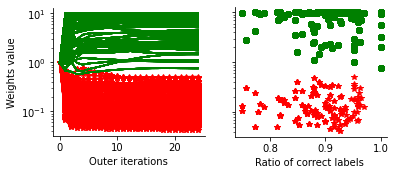
(a) For 30 standard trials

(b) For 3 standard trials

Figure 2: For each figure, on the left we find the evolution of weights for each comparison, over the outer iterations. In green the correct labels and in red the noisy ones. It is noticeable that incorrect observations attain values lower than one, while correct ones tend to $1/\epsilon$. On the right, each point represents the final weight of pair $i$ versus the ratio of correct labels over all available labels of pair $i$.

3.3.3 Application of PDHG

Problem (10) is in the form of (7), so we can directly apply the steps in (LABEL:eq:PDHG_algo). The proximal operators are given in Proposition 1, with the respective proof found in Appendix D.

Proposition 1.

The proximal operators $\textrm{prox}_{\tau f}(x)$ and $\textrm{prox}_{\sigma g^{*}}(x)$ of functions $f$ as defined in (11) and $g$ as defined in (9) are respectively given as

$$\begin{split}\textrm{prox}_{\tau f}(x)&=x^{\prime}-\bar{\textbf{x}^{\prime}}\\ \textrm{prox}_{\sigma g^{*}}(x)&=x-\tau(\textrm{prox}_{\tilde{w}_{n}\tilde{g}_{n}}(\tilde{x}_{n}))_{n=1}^{N},\end{split}$$

where $x^{\prime}=\frac{x}{1+2\gamma}$, $\bar{\textbf{x}}$ is the mean value of $x$, $\tilde{x}_{n}=x_{n}/\sigma$, $\tilde{w}_{n}=w_{n}/\sigma$ and $(f_{n}(x_{n}))_{n=1}^{N}$ is defined as the concatenation of function $f_{n}$ evaluated at component $n$ of $x$, for its N elements. Furthermore, $\textrm{prox}_{\tilde{w}_{n}\tilde{g}_{n}}(\tilde{x}_{n})$ is the solution of the following equation

$$\frac{-e^{1-u}}{1+e^{1-u}}+\frac{u-\tilde{x}_{n}}{\tilde{w}_{n}}=0.$$

4 Experiments

We split this section into 3 different parts. In Section 4.1, we focus on the internal behavior of our algorithm, looking at the weights and the stopping criteria for each stage of our algorithm. In Section 4.2, we compare our method with the state-of-the-art, simulating data according to different models. In Section 4.3 we test the methods with real-world data.

4.1 Performance of the algorithm

Setting.

We generate simulated data with $m$ items, where the ranking corresponds to a random permutation of integers between $1$ and $m$. Then, we randomly select $n$ pairs, with the possibility of selecting repeated pairs. For each pair we take its true label $y_{n}^{TRUE}$ and create a noisy one by multiplying toggle noise with probability $\delta_{n}$. The standard setting for all experiments considers 16 items, with $\delta_{n}=0.1$. The regularization weight $\gamma$ is set to $0.01$. We express the number of observations $n$ in terms of standard trials. One standard trial corresponds to all possible pairings of the $m$ items, given as $m(m-1)/2$. Note that due to repetitions 1 standard trial does not necessarily mean that we observe all possible pairs. For each simulation, we run 100 Monte Carlo trials. When appropriate we compare our algorithm with the solution obtained from a standard solver – CVXPY [18] – iteratively applied to Problem (5).

Weights as a measure of confidence.

We first look into the evolution of weights over the outer iterations. Figure 2 shows two distinct situations. The first exemplifies a scenario where there are enough comparisons to produce a completely accurate ranking. In this case, all incorrect labels have a weight lower than one and vice-versa. The second scenario contemplates fewer observations and we can see that some of the pairs have incorrect weights. Nonetheless, we see that their value is in general closer to 1 than to the extremities, thus providing a measure of uncertainty.

Stopping criteria.

The stopping criterion for the PDHG algorithm (i.e. the inner cycle) is taken as the difference in cost between consecutive iterations, as a fraction of the first, smaller than $\epsilon_{in}$. For the outer cycle, we take either the stabilization of the weight values or the existence of a large enough interval around 1 for their values, corresponding to the two situations in Figure 2. In Figure 3, we can see that $\epsilon_{in}$ has a large impact on the computation time of our algorithm, but it can be increased up to $0.01$ with minimal decrease in the accuracy. It is also evident the advantage we obtain in using our algorithm compared to a naive implementation.

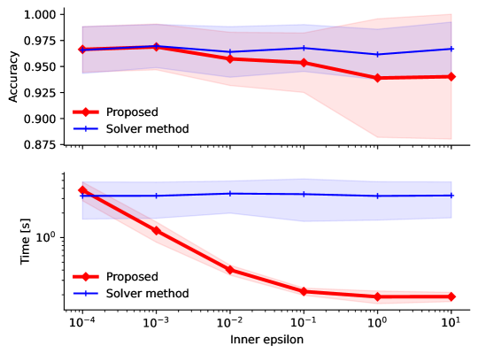
Figure 3: Variation of label accuracy and total computation time with $\epsilon_{in}$. The top figure depicts the accuracy of predicted labels for each observation with respect to the true labels. The shaded area corresponds to $1$ standard deviation.

4.2 Simulated data

Setting.

When testing with simulated data, we wish to compare methods with different underlying assumptions. Therefore, we compare against Borda Count [35], Bradley-Terry (BT) [6] and SVM-RankAggregation [32]. We also run simulations with data produced both according to the scores independent noise model (Section 2.1) and to the BT, where noise is correlated with the scores, with the remaining setting equal to the previous section. Since we do not aim at retrieving the correct rating score, but only the ranking, we choose Kendall’s Tau coefficient as a metric of closeness between the achieved and true ranking. Given the ground truth ranking ($r_{GT}$) and the resulting order given by each method ($r_{pred}$), Kendall’s tau is given as

$$\tau(r_{GT},r_{pred})=\frac{P-Q}{P+Q}$$

where $P$ is the number of concordant pairs and $Q$ the number of discordant pairs. A value closer to $1$ implies a better predicted ranking.

Simulations.

The results from simulations with the noise independent of scores can be found in Figure 4. We see that PD-Rank particularly stands out in moderate values of $n$, between 1 and 6 standard trials, while for very high values most models show similar performance except for the Borda Count. When it comes to noise variation, the larger advantage is seen up to $\delta=0.2$, after this point BT provides similar performance, but both still show a better ranking than SVM and Borda.

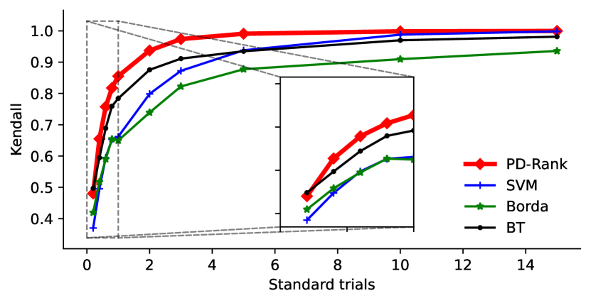
(a) Variation with number of comparisons

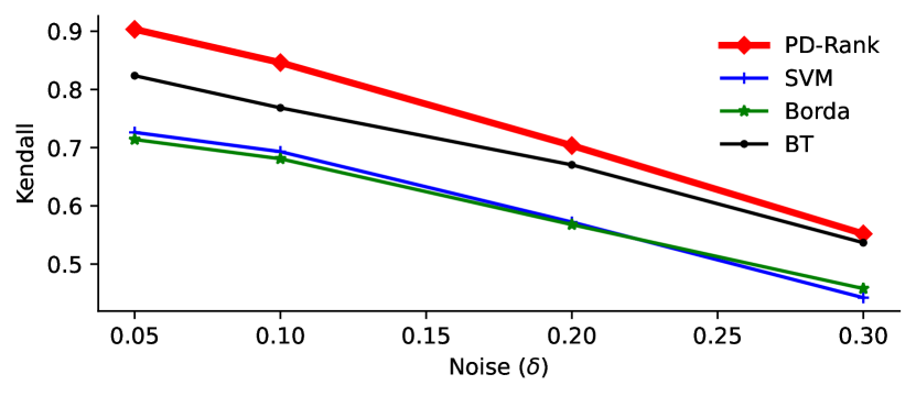
(b) Variation with noise level

Figure 4: Kendall coefficient for simulated data with noise independent of scores.

Given that the data in the latter experiment was produced according to the assumptions in our model, a better performance from PD-Rank was expected. So, in Figure 5, we show the results of simulations with data from the BT model. Even in this case, PD-Rank has a similar or higher performance than BT for lower values of comparisons. This makes it highly suitable for a large data setting, where a limited amount of labels can be obtained, often smaller than one standard trial. For a larger number of comparisons, BT is the best performer, particularly in closer score values.

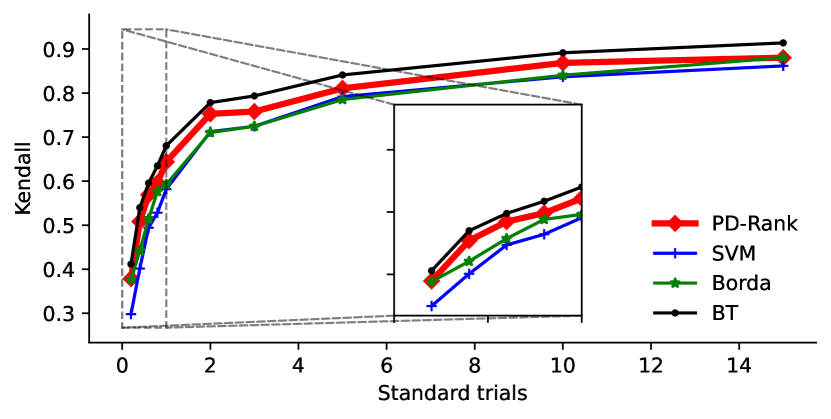
(a) BT model: scores 1 to 5

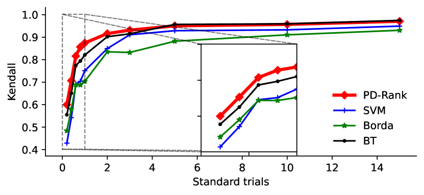
(b) BT model: scores 1 to 20

Figure 5: Kendall coefficient for simulated data according to the BT model. For the BT model, the value of scores influences the number of noisy observations, in the same way as of our $\delta$, and so we test for a small range and a larger one.

Large data scenario.

For the large data scenario, we want to see how PD-Rank handles an increase in $m$ and low values of $n$. For comparison, we will take the Borda Count, due to its extremely low computational complexity and Multistage Sorting (MS) [30], since it is also aimed at this setting and lies under the same data model. We increase the number of items $m$, while considering two settings for the observations: in the first $n$ increases as a fixed ratio ($0.1$) of the standard trial for the respective $m$, while in the second we keep $n$ fixed at an absolute value of $100000$. From a practical point of view, the latter is more realistic, as it is difficult to obtain the number of comparisons considered in the former. The results in Figure 6 show that PD-Rank scales very well with the number of items and tends to perform better in terms of Kendall coefficient, thus demonstrating its potential for ranking of datasets with a large collection of items.

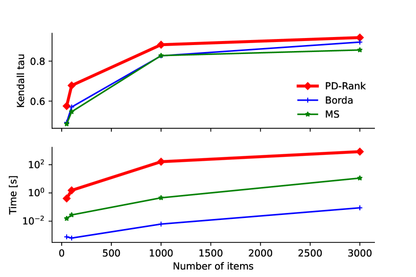
(a) Number of comparisons set to $0.1$ standard trial

(b) Number of comparisons set constant at $100000$

Figure 6: Large data setting, with variation of number of items $m$. On top we see the performance in terms of the Kendall coefficient and on the bottom the respective computation time.

4.3 Real-world datasets

Dataset description and setting.

We use two real-world common examples taken for the rank aggregation problem, for the pairwise comparison of distorted videos and images. The Image Quality Assessment (IQA) dataset is taken from the LIVE database [22] and [8] by the authors in [44] and the Video Quality Assessment(VQA) dataset from [28] by the authors in [42]. Both cases have original reference images or videos, respectively, with additional distorted versions, from which the authors produce a dataset of pairwise comparisons.

We compare PD-Rank with Borda Count (our implementation) and state-of-the-art active learning methods: Hodge-active [43] and Hybrid-MST [26] (authors implementation). Since there is no available ground truth (GT) for these datasets it is common practice to take GT as the ranking obtained with the full dataset (e.g. 32 standard trials for one IQA reference set). Note that we will take the BT solution as GT, as it is the golden standard, but this brings some unfairness to Borda Count and PD-Rank, as they are usually not able to reach Kendall of 1.0, since the GT according to all methods is not the same.

Simulations.

Figure 7 depicts the results for Reference 1 of IQA dataset. PD-Rank is the best option in computation time if one wishes to achieve higher accuracy with less computational time. Active learning methods arrive at a higher Kendall with less available comparisons, but they require more time, as they must be run sequentially. Borda Count is always faster than any other candidate but it requires a much larger data sample, being a better option for cases where it is easy to retrieve multiple standard trials.

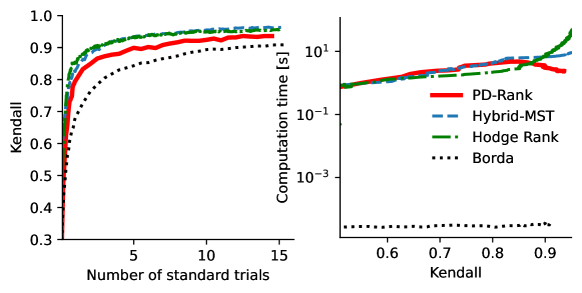
Figure 7: Results for Reference 1 of IQA-dataset. On the left plot, we can see the evolution of ranking accuracy with the observed samples. On the right we show the evolution of computation time with the achieved Kendall coefficient: lines above PD-Rank require more time for the same accuracy and vice-versa.

5 Conclusion

We defined a new model for the ranking problem, leading to a non-convex and discontinuous optimization problem. We obtained a continuous nonconvex approximation and solved it with PD-Rank, an algorithm based on iteratively re-weighted minimization and the Primal-Dual Hybrid Gradient. The method competes in accuracy with the state-of-the-art under simulated and real-world data experiments, and its speed makes PD-Rank particularly suitable for large data scenarios. Future directions include the study of theoretical guarantees regarding our approximation; the impact of including prior knowledge on annotator behavior and possibly the combination with active learning, especially taking advantage of the information provided by the confidence weights.

Appendix A Equivalence to 0-1 Loss

Considering that in (2.2) one of the indicator function terms will always be $1$ and the other $0$, we can reformulate the problem as

$$\begin{split}\operatornamewithlimits{maximize}\sum_{n=1}^{N}\mathbb{I}_{\mathrm{sign}(c_{n}^{T}x)}(y_{n})\log(1-\delta_{n})+\mathbb{I}_{-\mathrm{sign}(c_{n}^{T}x)}(y_{n})\log(\delta_{n})\end{split}$$

Besides, since $\mathbb{I}_{\mathrm{sign}(c_{n}^{T}x)}(y_{n})=\mathbb{I}_{\geq 0}(y_{n}c_{n}^{T}x)$ and $\mathbb{I}_{-\mathrm{sign}(c_{n}^{T}x)}(y_{n})=-\mathbb{I}_{\geq 0}(y_{n}c_{n}^{T}x)$, we can further obtain

$$\operatornamewithlimits{maximize}_{x}\sum_{n=1}^{N}\log\Big{(}\frac{1-\delta_{n}}{\delta_{n}}\Big{)}\mathbb{I}_{\geq 0}(y_{n}c_{n}^{T}x).$$

The previous maximization is naturally equivalent to

$$\operatornamewithlimits{minimize}_{x}\sum_{n=1}^{N}\log\Big{(}\frac{1-\delta_{n}}{\delta_{n}}\Big{)}(1-\mathbb{I}_{\geq 0}(y_{n}c_{n}^{T}x)),$$

which is the well-known 0-1 loss.

Appendix B Further insight into weights

Visual support for the explanation of the correspondence between $w$ and $\omega$ in Section 3.2.

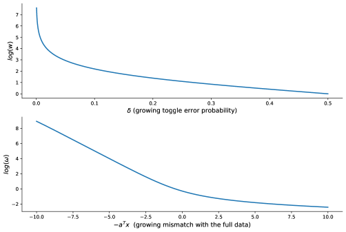
Figure 8: Comparison between variation of $w$ and $\omega$. On the top we vary $\delta$, the noise, between $0$ and $0.5$, depicting the correspondent evolution of $w$. On the bottom we vary the different between two items according to the proposed ranking, with the correponding $\omega$, according to (6).

Appendix C Existence and uniqueness of the minimizer of problem (5)

Proposition 2 (Existence and uniqueness of the minimizer of problem (5)).

Let problem (5), be one instance for a generic $k>0$, and define $\omega^{0}=(\omega_{1}^{0},\cdots,\omega_{N}^{0})$ as the vector collecting all the initialization weights for the iterative reweighting optimization scheme such that $\omega^{0}=\mathbf{1}$. Define the comparison noisy data $a_{n}=z_{n}c_{n}$, a small regularization constant $\gamma>0$, and $\omega_{n}^{k}$ defined as in (6).

Then, the $\operatornamewithlimits{argmin}$ set is a nonempty singleton set, i.e., problem (5) always has a solution and the solution is unique.

Proof.

The result follows easily from convexity of the summation terms, where $\omega_{n}^{k}\log\left(1+e^{1-a_{n}^{T}x}\right)$ is the product of a positive number and the convex log-sum-exp, and the $\gamma$-strong convexity of the second term $\gamma\|x\|^{2}_{2}$. ∎

Appendix D Proof of Proposition 1

We derive the proximal operators of $f(x)$ and $g^{*}(x)$ in subsections D.2 and D.3, respectively. For ease of the reader, in subsection D.1, we restate some basic background on proximal operators.

D.1 Proximal operators: background

Definition 1 (Proximal operator).

Given a function $f$, the proximal operator $\operatorname{prox}_{f}:\mathbb{R}^{n}\to\mathbb{R}^{n}$ of $f$ is defined as

$$\operatorname{prox}_{f}(x)=\operatornamewithlimits{argmin}_{u}\Big{(}f(u)+\frac{1}{2}\|u-x\|^{2}_{2}\Big{)}$$ (12)

and the proximal operator of the scaled function $\lambda f$, where $\lambda>0$ is expressed as

$$\operatorname{prox}_{\lambda f}(x)=\operatornamewithlimits{argmin}_{u}\Big{(}f(u)+\frac{1}{2\lambda}\|u-x\|^{2}_{2}\Big{)}.$$ (13)

Proposition 3 (Prox operator of the indicator function).

Given $f(x)=i_{C}(u)$, where $i_{C}(u)$ is the indicator function defined as

$$i_{S}(u)=\begin{cases}1&\mathrm{if}\quad u\in C\\ +\inf&\quad\mathrm{otherwise},\end{cases}$$ (14)

and $C$ is a nonempty, closed and convex set, the proximal operator of $f(x)$ exists and is unique, and it is given by the orthogonal projection operator onto the same set, denoted as $P_{C}(x)$, so

$$\operatorname{prox}_{f}(x)=P_{C}(x).$$ (15)

Proposition 4 (Prox operator with regularization).

Given $f(x)=\phi(x)+(\rho/2)\|x-a\|_{2}^{2}$, the proximal operator of $f(x)$ is given as

$$\operatorname{prox}_{\lambda f}(v)=\operatorname{prox}_{\tilde{\lambda}\phi}((\tilde{\lambda}/\lambda)v+(\rho\tilde{\lambda})a),$$ (16)

with $\tilde{\lambda}=\lambda/(1+\lambda\rho)$.

Proposition 5 (Prox operator of the Log-Sum-Exp function).

Given $f(x)=\log(1+e^{1-x})$, the proximal operator of $f$, $\operatorname{prox}_{\lambda f}(x)$, is given as the solution of the following equation with respect to $u$

$$\frac{-e^{1-u}}{1+e^{1-u}}+\frac{u-x}{\lambda}=0.$$ (17)

Note that the proximal operator is given by the minimization

$$\operatorname{prox}_{\lambda f}(x)=\operatornamewithlimits{argmin}_{u}\Big{(}\log(1+e^{1-u})+\frac{1}{2\lambda}\|u-x\|^{2}_{2}\Big{)}.$$ (18)

By taking the derivative of (18) with respect to $u$ and equating to $0$, we obtain (17).

D.2 Proximal operator of $f$

Proposition 6.

Given $f(x)$ defined as $f(x)=i_{\{u:\textbf{1}^{T}u=0\}}(x)$, where $i_{S}(u)$ is an indicator function of set $S$, as defined in (14), the proximal operator of $f(x)$ is given as

$$\operatorname{prox}_{f}(x)=x-\bar{\textbf{x}},$$ (19)

where $\bar{x}$ is the mean of $x$.

By (15), the proximal operator of an indicator function is given as

$$\operatorname{prox}_{f}(x)=P_{S}(x).$$

In this case $S=\{u:\textbf{1}^{T}u=0\}$, so this is an affine set. It is known that the orthogonal projection onto an affine set $C_{1}=\{u:Au=b\}$ is given as

$$P_{C_{1}}(x)=x-A^{T}(AA^{T})^{-1}(Ax-b).$$

Taking $A=\textbf{1}^{T}$ and $b=0$, we obtain

$$P_{S}(x)=x-\textbf{1}\Big{[}\frac{\textbf{1}^{T}x}{M}\Big{]},$$

where we note that the second term is the mean of x, denoted as $\bar{x}$. Consequently, we have

$$\operatorname{prox}_{f}(x)=x-\bar{\textbf{x}}.$$

Now, taking $g(x)=f(x)+\gamma\|x\|_{2}^{2}$ and by (16), the proximal operator of $g(x)$ is given as

$$\operatorname{prox}_{g}(x)=\operatorname{prox}_{f}\Bigg{(}\frac{1}{1+2\gamma}x\Bigg{)}.$$

D.3 Proximal operator of $g^{*}(x)$

Proposition 7.

Given $g(x)$ defined as $g(x)=\sum_{n=1}^{N}w_{n}\textrm{LSE}(1-e_{n}^{T}x)$, where $\textrm{LSE}(t)=\log(1+e^{t})$, the proximal operator of the conjugate function $g^{*}(x)$ is given as

$$\operatorname{prox}_{\tau g^{*}}(x)=x-\tau(\operatorname{prox}_{\tilde{w}_{n}\tilde{g}_{n}}(\tilde{x}_{n}))_{n=1}^{N},$$ (20)

where $\tilde{x}_{n}=x_{n}/\tau$, $\tilde{w}_{n}=w_{n}/\tau$, $\tilde{g}_{n}(y_{n})=\textrm{LSE}(1-y_{n})$, and $\textrm{prox}_{\tilde{w}_{n}\tilde{g}_{n}}(\tilde{x}_{n})$ is the solution of

$$\frac{-e^{1-u}}{1+e^{1-u}}+\frac{u-\tilde{x}_{n}}{\tilde{w}_{n}}=0$$

with respect to $u$.

By Moreau decomposition (see [3], for instance), we have that

$$\operatorname{prox}_{\tau g^{*}}(x)=x-\tau\operatorname{prox}_{\tau^{-1}g}(x/\tau).$$

and since $g$ is separable we have

$$\operatorname{prox}_{\tau g^{*}}(x)=x-\tau(\operatorname{prox}_{\tau^{-1}g_{n}}(x_{n}/\tau))_{n=1}^{N},$$

where $g_{n}(y_{n})=w_{n}\textrm{LSE}(1-y_{n})$. Then, for each component, we have that

$$\operatorname{prox}_{\tau^{-1}g_{n}}(x_{n}/\tau)=\operatorname{prox}_{w_{n}/\tau\tilde{g}_{n}}(x_{n}/\tau),$$

where $\tilde{g}_{n}(y_{n})=\textrm{LSE}(1-y_{n})$ and $w_{n}>0$. Then, defining $x_{n}/\tau$ as $\tilde{x}_{n}$ and $w_{n}/\tau$ as $\tilde{w}_{n}$, we can obtain

$$\operatorname{prox}_{\tilde{w}_{n}\tilde{g}_{n}}(\tilde{x}_{n})$$

from the solution of Equation 17.Therefore, we have that

$$\operatorname{prox}_{\tau g^{*}}(x)=x-\tau(\operatorname{prox}_{\tilde{w}_{n}\tilde{g}_{n}}(\tilde{x}_{n}))_{n=1}^{N}.$$

Appendix E Additional Experiments

We include some additional references for datasets VQA (Figure 9) and IQA (Figure 10), that reinforce the conclusions obtained in the main paper. Recall that we are taking as ground truth (GT) the solution obtained with the Bradley-Terry model for the full dataset and this brings some unfairness to Borda Count and PD-Rank, as they are usually not able to reach Kendall of 1.0, since the GT according to all methods is not the same. We confirm that for higher accuracies (over $0.85$) PD-rank achieves the same Kendall as Hybrid-MST and Hodge Rank with less computation time. The latter two, being active learning methods arrive at a higher Kendall tau with less available comparisons, but they require more time, as they must be run sequentially. Borda Count is always faster than any other candidate by several orders of magnitude, but it requires a much larger data sample and often does not reach high enough values of Kendall tau.

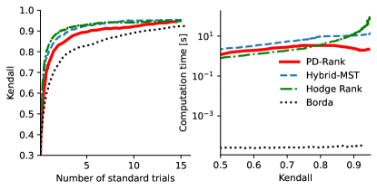
(a)

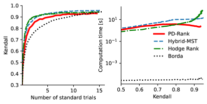
(b)

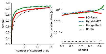
(c)

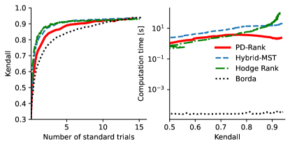
(d)

Figure 9: Additional results for simulations with VQA-dataset. For each subfigure, on the left plot, we can see the evolution of ranking accuracy with the observed samples. Observed samples are expressed in terms of standard trials, where 1 standard trial is defined as $m(m-1)/2$, for $m$ items. On the right, we show the evolution of computation time with the achieved Kendall coefficient: lines above PD-Rank require more time for the same accuracy and vice-versa.

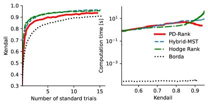
(a)

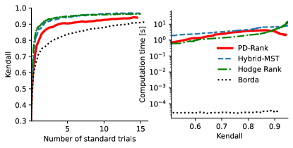
(b)

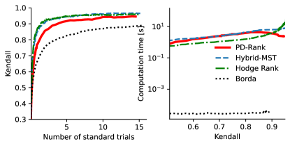
(c)

(d)

Figure 10: Additional results for simulations with IQA-dataset. For each subfigure, on the left plot, we can see the evolution of ranking accuracy with the observed samples. Observed samples are expressed in terms of standard trials, where 1 standard trial is defined as $m(m-1)/2$, for $m$ items. On the right, we show the evolution of computation time with the achieved Kendall coefficient: lines above PD-Rank require more time for the same accuracy and vice-versa.

References

- [1] A. Agarwal, S. Agarwal, S. Khanna, and P. Patil, Rank aggregation from pairwise comparisons in the presence of adversarial corruptions, in Proceedings of the 37th International Conference on Machine Learning, vol. 119, PMLR, 13–18 Jul 2020, pp. 85–95.
- [2] P. L. Bartlett, M. I. Jordan, and J. D. McAuliffe, Convexity, classification, and risk bounds, Journal of the American Statistical Association, 101 (2006), pp. 138–156.
- [3] A. Beck, Chapter 6: The Proximal Operator, Society for Industrial and Applied Mathematics, Philadelphia, PA, 2017, pp. 129–177.
- [4] J. M. Bioucas-Dias and M. A. T. Figueiredo, A new twist: Two-step iterative shrinkage/thresholding algorithms for image restoration, IEEE Transactions on Image Processing, 16 (2007), pp. 2992–3004.
- [5] S. Bozóki, L. Csato, and J. Temesi, An application of incomplete pairwise comparison matrices for ranking top tennis players, European Journal of Operational Research, 248 (2016), pp. 211–218.
- [6] R. A. Bradley and M. E. Terry, Rank analysis of incomplete block designs: I. the method of paired comparisons, Biometrika, 39 (1952), pp. 324–345.
- [7] M. Braverman and E. Mossel, Noisy sorting without resampling, Proceedings of the Annual ACM-SIAM Symposium on Discrete Algorithms, (2007).
- [8] P. L. Callet and F. Autrusseau, Subjective quality assessment irccyn/ivc database. http://www.irccyn.ec-nantes.fr/ivcdb/, 2005.
- [9] Z. Cao, T. Qin, T.-Y. Liu, M.-F. Tsai, and H. Li, Learning to rank: From pairwise approach to listwise approach, in Proceedings of the 24th International Conference on Machine Learning, vol. 227, 01 2007, pp. 129–136.
- [10] R. Chartrand and W. Yin, Iteratively reweighted algorithms for compressive sensing, in 2008 IEEE International Conference on Acoustics, Speech and Signal Processing, 2008, pp. 3869–3872.
- [11] X. Chen, P. Bennett, K. Collins-Thompson, and E. Horvitz, Pairwise ranking aggregation in a crowdsourced setting, in WSDM 2013 - Proceedings of the 6th ACM International Conference on Web Search and Data Mining, 02 2013, pp. 193–202.
- [12] X. Chen, Y. Li, and J. Mao, A nearly instance optimal algorithm for top-k ranking under the multinomial logit model, in Proceedings of the Twenty-Ninth Annual ACM-SIAM Symposium on Discrete Algorithms, SODA ’18, USA, 2018, Society for Industrial and Applied Mathematics, p. 2504–2522.
- [13] Y. Chen and C. Suh, Spectral MLE: Top-K rank aggregation from pairwise comparisons, in 32nd International Conference on Machine Learning, 2015, pp. 371–380.
- [14] M. Condorcet, Éssai sur l’application de l’analyse à la probabilité des décisions rendues à la pluralité des voix, l’Imprimerie Royale, Paris, (1785).
- [15] I. Daubechies, R. DeVore, M. Fornasier, and C. S. Gü ntürk, Iteratively reweighted least squares minimization for sparse recovery, Communications on Pure and Applied Mathematics: A Journal Issued by the Courant Institute of Mathematical Sciences, 63 (2010), pp. 1–38.
- [16] I. Daubechies, R. DeVore, M. Fornasier, and S. Gunturk, Iteratively re-weighted least squares minimization: Proof of faster than linear rate for sparse recovery, in 2008 42nd Annual Conference on Information Sciences and Systems, 2008, pp. 26–29.
- [17] J. de Borda, Mémoire sur les élections au scrutin, Histoire de l’Académie Royale des Sciences, Paris, (1781).
- [18] S. Diamond and S. Boyd, CVXPY: A Python-embedded modeling language for convex optimization, Journal of Machine Learning Research, 17 (2016), pp. 1–5.
- [19] E. Esser, X. Zhang, and T. Chan, A general framework for a class of first order primal-dual algorithms for convex optimization in imaging science, SIAM Journal of Imaging Sciences, 3 (2010), pp. 1015–1046.
- [20] D. Fotakis, A. Kalavasis, and K. Stavropoulos, Aggregating incomplete and noisy rankings, in 24th International Conference on Artificial Intelligence and Statistics, 2021.
- [21] R. Freedman, J. Schaich Borg, W. Sinnott-Armstrong, J. Dickerson, and V. Conitzer, Adapting a kidney exchange algorithm to align with human values, Artificial Intelligence, 283 (2020), p. 103261.
- [22] L. C. H. Sheikh, Z. Wang and A. Bovik, Live image quality assessment database release 2. http://live.ece.utexas.edu/research/quality, 2008.
- [23] R. Heckel, N. B. Shah, K. Ramchandran, and M. J. Wainwright, Active ranking from pairwise comparisons and when parametric assumptions do not help, The Annals of Statistics, 47 (2019), pp. 3099 – 3126.
- [24] J. Hu and P. Li, Improved and scalable bradley-terry model for collaborative ranking, in 2016 IEEE 16th International Conference on Data Mining (ICDM), 2016, pp. 949–954.
- [25] A. Karatzoglou, L. Baltrunas, and Y. Shi, Learning to rank for recommender systems, in RecSys 2013 - Proceedings of the 7th ACM Conference on Recommender Systems, 10 2013, pp. 493–494.
- [26] J. Li, R. K. Mantiuk, J. Wang, S. Ling, and P. L. Callet, Hybrid-MST: A hybrid active sampling strategy for pairwise preference aggregation, in Proceedings of the 32nd International Conference on Neural Information Processing Systems, 2018, p. 3479–3489.
- [27] K. Li, X. Zhang, and G. Li, A rating-ranking method for crowdsourced top-k computation, 05 2018, pp. 975–990.
- [28] LIVE video quality assessment database. http://live.ece.utexas.edu/research/quality/, 2008.
- [29] Z. Lu, Iterative reweighted minimization methods for lp regularized unconstrained nonlinear programming, Mathematical Programming, 147 (2014), pp. 277–307.
- [30] C. Mao, J. Weed, and P. Rigollet, Minimax rates and efficient algorithms for noisy sorting, in Proceedings of Algorithmic Learning Theory, 2018, pp. 821–847.
- [31] D. Park, J. Neeman, J. Zhang, S. Sanghavi, and I. Dhillon, Preference completion: Large-scale collaborative ranking from pairwise comparisons, in Proceedings of the 32nd International Conference on Machine Learning, vol. 37, 07 2015, pp. 1907–1916.
- [32] A. Rajkumar and S. Agarwal, A statistical convergence perspective of algorithms for rank aggregation from pairwise data, in Proceedings of the 31st International Conference on Machine Learning, vol. 1, 01 2014, pp. 206–227.
- [33] T. L. Saaty, A scaling method for priorities in hierarchical structures, Journal of Mathematical Psychology, 15 (1977), pp. 234–281.
- [34] P. Salesses, K. Schechtner, and C. Hidalgo, The collaborative image of the city: Mapping the inequality of urban perception, PLoS ONE, 8 (2013), p. e68400.
- [35] N. B. Shah and M. J. Wainwright, Simple, robust and optimal ranking from pairwise comparisons, Journal of Machine Learning Research, 18 (2018), pp. 1–38.
- [36] E. Simpson and I. Gurevych, Scalable Bayesian preference learning for crowds, Machine Learning, 109 (2020), pp. 689–718.
- [37] C. N. Stewart N, Brown GD, Absolute identification by relative judgment, Psychological Review, 112(4) (2005), pp. 881–911.
- [38] C. Suh, V. Y. F. Tan, and R. Zhao, Adversarial top-K ranking, IEEE Transactions on Information Theory, 63 (2017), pp. 2201–2225.
- [39] L. L. Thurstone, A law of comparative judgment, Psychological Review, 34 (1927), pp. 273–286.
- [40] H. Wang, G. Kou, and Y. Peng, An iterative algorithm to derive priority from large-scale sparse pairwise comparison matrix, IEEE Transactions on Systems, Man, and Cybernetics: Systems, (2021), pp. 1–14.
- [41] F. Wauthier, M. Jordan, and N. Jojic, Efficient ranking from pairwise comparisons, in Proceedings of the 30th International Conference on Machine Learning, vol. 28 of Proceedings of Machine Learning Research, 2013, pp. 109–117.
- [42] Q. Xu, T. Jiang, Y. Yao, Q. Huang, B. Yan, and W. Lin, Random partial paired comparison for subjective video quality assessment via hodgerank, in Proceedings of the 19th ACM international conference on Multimedia, 11 2011, pp. 393–402.
- [43] Q. Xu, J. Xiong, X. Chen, and Y. Yao, HodgeRank with information maximization for crowdsourced pairwise ranking aggregation, in Proceedings of the Thirty-Second AAAI Conference on Artificial Intelligence and Thirtieth Innovative Applications of Artificial Intelligence Conference and Eighth AAAI Symposium on Educational Advances in Artificial Intelligence, 11 2018.
- [44] P. Ye and D. Doermann, Active sampling for subjective image quality assessment, in Proceedings of the IEEE Computer Society Conference on Computer Vision and Pattern Recognition, 06 2014, pp. 4249–4256.