Abstract

In gauge-Higgs unification (GHU), gauge symmetry is dynamically broken by an Aharonov-Bohm (AB) phase, $\theta_{H}$, in the fifth dimension. We analyze $SU(2)$ GHU with an $SU(2)$ doublet fermion in flat $M^{4}\times(S^{1}/Z_{2})$ spacetime and in the Randall-Sundrum (RS) warped space. With orbifold boundary conditions the $U(1)$ part of gauge symmetry remains unbroken at $\theta_{H}=0$ and $\pi$. The fermion multiplet has chiral zero modes at $\theta_{H}=0$, which become massive at $\theta_{H}=\pi$. In other words chiral fermions are transformed to vectorlike fermions by the AB phase $\theta_{H}$. Chiral anomaly at $\theta_{H}=0$ continuously varies as $\theta_{H}$ and vanishes at $\theta_{H}=\pi$. We demonstrate this intriguing phenomenon in the RS space in which there occurs no level crossing in the mass spectrum and everything varies smoothly. The flat spacetime limit is singular as the AdS curvature of the RS space diminishes, and reproduces the result in the flat spacetime. Anomalies appear for various combinations of Kaluza-Klein excitation modes of gauge fields as well. Although the magnitude of anomalies depends on $\theta_{H}$ and the warp factor of the RS space, it does not depend on the bulk mass parameter of the fermion field controlling its mass and wave function at general $\theta_{H}$.

1 Introduction

In gauge-Higgs unification (GHU), gauge symmetry is dynamically broken by an Aharonov-Bohm (AB) phase, $\theta_{H}$, in the fifth dimension.[1]-[7] In the analysis of finite temperature behavior of grand unified theory (GUT) inspired $SO(5)\times U(1)_{X}\times SU(3)_{C}$ GHU models in the Randall-Sundrum (RS) warped space, it has been observed that chiral quarks and leptons at $\theta_{H}=0$ are transformed to vectorlike fermions at $\theta_{H}=\pi$.[8] As $\theta_{H}$ varies from 0 to $\pi$, $SU(2)_{L}\times U(1)_{Y}\times SU(3)_{C}$ gauge symmetry is smoothly converted to $SU(2)_{R}\times U(1)_{Y^{\prime}}\times SU(3)_{C}$ gauge symmetry. Chiral fermions appearing as zero modes of fermion multiplets in the spinor representation of $SO(5)$ at $\theta_{H}=0$ become massive fermions having vectorlike gauge couplings at $\theta_{H}=\pi$.

Chiral fermions in four dimensions, in general, give rise to chiral anomalies.[9, 10, 11] What would be a fate of those anomalies if fermions are converted to massive vectorlike fermions at $\theta_{H}=\pi$? Do anomalies disappear as $\theta_{H}$ changes from 0 to $\pi$? How can it happen? These are the questions and issues addressed in this paper.

To keep arguments in clarity, we analyze $SU(2)$ GHU with an $SU(2)$ doublet fermion both in flat $M^{4}\times(S^{1}/Z_{2})$ spacetime and in the RS warped space with orbifold boundary conditions breaking $SU(2)$ to $U(1)$. We shall see that $U(1)$ gauge symmetry survives at $\theta_{H}=0$ and $\pi$, and that the fermion multiplet has chiral zero modes at $\theta_{H}=0$ which become massive at $\theta_{H}=\pi$. We determine 4D couplings of all Kaluza-Klein (KK) modes of gauge fields and fermion fields at general $\theta_{H}$, and evaluate triangle chiral anomalies.

In the flat $M^{4}\times(S^{1}/Z_{2})$ spacetime all gauge couplings are determined analytically, but the mass spectrum of gauge and fermion fields exhibit level crossing as $\theta_{H}$ varies. In the RS spacetime there occurs no level crossing in the spectrum, and gauge couplings are evaluated numerically. It will be seen that 4D gauge couplings of fermions in the RS space smoothly changes as $\theta_{H}$, and that the chiral anomaly associated with the zero mode of gauge fields at $\theta_{H}=0$ smoothly varies and vanishes at $\theta_{H}=\pi$. The flat space limit gives singular behavior of the anomaly as a function of $\theta_{H}$, reproducing the analytical result in the flat spacetime. We will also see that anomalies appear in various combinations of KK modes of gauge fields.

In Section 2 $SU(2)$ GHU models are introduced both in flat $M^{4}\times(S^{1}/Z_{2})$ spacetime and in the RS space. As functions of the AB phase $\theta_{H}$ the mass spectra of KK modes of gauge and fermion fields are obtained. It will be seen that there occurs no level crossing in the spectrum in the RS space. In Section 3 gauge couplings and anomalies are evaluated in the flat $M^{4}\times(S^{1}/Z_{2})$ spacetime. In Section 4 gauge couplings and anomalies are evaluated in the RS space. It is shown that the magnitude of anomalies smoothly changes as $\theta_{H}$. The dependence of those anomalies on the warp factor $z_{L}$ of the RS space and the bulk mass parameter $c$ of fermion fields is also investigated. It is seen that the flat space limit $z_{L}\rightarrow 1$ of anomalies is singular. It is also seen by numerical evaluation that the magnitude of anomalies does not depend on the bulk mass parameter $c$. Section 5 is devoted to a summary and discussion.

2 $SU(2)$ GHU models

The action in $SU(2)$ GHU in flat $M^{4}\times(S^{1}/Z_{2})$ spacetime with coordinate $x^{M}$ ($M=0,1,2,3,5$, $x^{5}=y$) is given by

$$I_{\rm flat} =\int d^{4}x\int_{0}^{L}dy\,{\cal L}_{\rm flat}~{},$$ (2.1)

$${\cal L}_{\rm flat} =-\frac{1}{2}{\rm Tr}\,F_{MN}F^{MN}+\overline{\Psi}\gamma^{M}D_{M}\Psi+\overline{\Psi}{}^{\prime}\gamma^{M}D_{M}\Psi^{\prime}~{},$$ (2.2)

where ${\cal L}_{\rm flat}(x^{\mu},y)={\cal L}_{\rm flat}(x^{\mu},-y)={\cal L}_{\rm flat}(x^{\mu},y+2L)$. Here $F_{MN}=\partial_{M}A_{N}-\partial_{N}A_{N}-ig_{A}[A_{M},A_{N}]$, $A_{M}=\hbox{$\frac{1}{2}$}\sum_{a=1}^{3}A^{a}_{M}\tau^{a}$ where $\tau^{a}$’s are Pauli matrices. We have introduced two types of $SU(2)$ doublet fermions $\Psi,\Psi^{\prime}$ with $D_{M}=\partial_{M}-ig_{A}A_{M}$. The metric is $\eta_{MN}={\rm diag}\,(-1,1,1,1,1)$ and $\overline{\Psi}=i\Psi^{\dagger}\gamma^{0}$. Orbifold boundary conditions are given, with $(y_{0},y_{1})=(0,L)$, by

$$\begin{pmatrix}A_{\mu}\cr A_{y}\end{pmatrix}(x,y_{j}-y) =P_{j}\begin{pmatrix}A_{\mu}\cr-A_{y}\end{pmatrix}(x,y_{j}+y)P_{j}^{-1}~{},$$ (2.3)

$$\Psi(x,y_{j}-y) =P_{j}\gamma^{5}\Psi(x,y_{j}+y)~{},$$ (2.4)

$$\Psi^{\prime}(x,y_{j}-y) =(-1)^{j}P_{j}\gamma^{5}\Psi^{\prime}(x,y_{j}+y)~{},$$ (2.5)

$$P_{0}=P_{1} =\tau^{3}~{}.$$ (2.6)

The $SU(2)$ symmetry is broken to $U(1)$ by the boundary conditions (2.6). $A^{3}_{\mu},A^{1,2}_{y}$ are parity even at both $y_{0}$ and $y_{1}$, and have constant zero modes. Let us denote doublet fields as $\Psi=(u,d)^{t}$ and $\Psi^{\prime}=(u^{\prime},d^{\prime})^{t}$. $u_{R}$ and $d_{L}$ are parity even at both $y_{0}$ and $y_{1}$, and have zero modes, leading to chiral structure.

The KK expansions of gauge fields around the configuration $A_{M}=0$ are given, with $L=\pi R$, by

$$A_{\mu}^{1,2}(x,y) =\sqrt{\frac{2}{\pi R}}\sum_{n=1}^{\infty}A_{\mu}^{1,2\,(n)}(x)\,\sin\frac{ny}{R}~{},$$ (2.7)

$$A_{\mu}^{3}(x,y) =\frac{1}{\sqrt{\pi R}}A_{\mu}^{3\,(0)}(x)+\sqrt{\frac{2}{\pi R}}\sum_{n=1}^{\infty}A_{\mu}^{3\,(n)}(x)\,\cos\frac{ny}{R}~{},$$ (2.8)

$$A_{y}^{1,2}(x,y) =\frac{1}{\sqrt{\pi R}}A_{y}^{1,2\,(0)}(x)+\sqrt{\frac{2}{\pi R}}\sum_{n=1}^{\infty}A_{y}^{1,2\,(n)}(x)\,\cos\frac{ny}{R}~{},$$ (2.9)

$$A_{y}^{3}(x,y) =\sqrt{\frac{2}{\pi R}}\sum_{n=1}^{\infty}A_{y}^{3\,(n)}(x)\,\sin\frac{ny}{R}~{}.$$ (2.10)

Gauge coupling of 4D $U(1)$ gauge fields $A_{\mu}^{3\,(0)}(x)$ is given by

$$g_{4}=\frac{g_{A}}{\sqrt{L}}~{}.$$ (2.11)

The zero modes $A_{y}^{1,2\,(0)}$ may develop a nonvanishing expectation value, which leads to an AB phase $\theta_{H}$ along the fifth dimension. Without loss of generality one may assume that $\langle A_{y}^{1\,(0)}\rangle=0$. Then

$$P\exp\bigg{\{}ig_{A}\int_{0}^{2L}dy\,\langle A_{y}\rangle\bigg{\}}=e^{i\theta_{H}\tau^{2}}=\begin{pmatrix}\cos\theta_{H}&\sin\theta_{H}\cr-\sin\theta_{H}&\cos\theta_{H}\end{pmatrix}~{},$$ (2.12)

$$\theta_{H}=g_{4}L\,\langle A_{y}^{2\,(0)}\rangle~{}.$$ (2.13)

The AB phase $\theta_{H}$ is a physical quantity. It couples to fields, affecting their mass spectrum. It will be shown shortly that the mode expansions in (2.10) do not correspond to mass eigenstates for $\theta_{H}\not=0$ and need to be improved.

One can change the value of $\theta_{H}$ by a gauge transformation, which also alters boundary conditions. Consider a large gauge transformation given by

$$\tilde{A}_{M} =\Omega A_{M}\Omega^{-1}+\frac{i}{g_{A}}\Omega\partial_{M}\Omega^{-1}~{},~{}~{}\tilde{\Psi}=\Omega\Psi~{},~{}~{}\tilde{\Psi}^{\prime}=\Omega\Psi^{\prime}~{},$$ (2.14)

$$\Omega =\exp\Big{(}\frac{i}{2}\theta(y)\tau^{2}\Big{)}~{},~{}~{}\theta(y)=\theta_{H}\Big{(}1-\frac{y}{L}\Big{)}$$ (2.15)

under which $\tilde{\theta}_{H}=0$ and boundary condition matrices become

$$\tilde{P}_{j} =\Omega(y_{j}-y)P_{j}\Omega^{-1}(y_{j}+y)~{},$$ (2.16)

$$\tilde{P}_{0} =\begin{pmatrix}\cos\theta_{H}&-\sin\theta_{H}\cr-\sin\theta_{H}&-\cos\theta_{H}\end{pmatrix},~{}~{}\tilde{P}_{1}=\tau^{3}~{}.$$ (2.17)

Although the AB phase $\tilde{\theta}_{H}$ vanishes, boundary conditions become nontrivial. Physics remains the same. This gauge is called the twisted gauge.[12, 13]

In the twisted gauge $\tilde{\theta}_{H}=0$ so that fields satisfy free equations. The boundary condition at $y=L$ remains the same as in the original gauge so that mode functions take the form

$$\tilde{P}_{1}=+ :\quad C_{\lambda}(y)=\cos\lambda(y-L)~{},$$ (2.18)

$$\tilde{P}_{1}=- :\quad S_{\lambda}(y)=\sin\lambda(y-L)~{}.$$ (2.19)

At $y=0$, $\tilde{A}_{\mu}^{1}$ and $\tilde{A}_{\mu}^{3}$ intertwine with each other. Their general eigenmodes can be written in the form

$$\begin{pmatrix}\tilde{A}_{\mu}^{1}\cr\tilde{A}_{\mu}^{3}\end{pmatrix} =\begin{pmatrix}\alpha S_{\lambda}(y)\cr\beta C_{\lambda}(y)\end{pmatrix}B_{\mu}^{(\lambda)}(x)~{}.$$ (2.20)

Note that

$$\begin{pmatrix}A_{\mu}^{1}\cr A_{\mu}^{3}\end{pmatrix} =\begin{pmatrix}\cos\theta(y)&\sin\theta(y)\cr-\sin\theta(y)&\cos\theta(y)\end{pmatrix}\begin{pmatrix}\tilde{A}_{\mu}^{1}\cr\tilde{A}_{\mu}^{3}\end{pmatrix}~{}.$$ (2.21)

Hence the boundary conditions at $y=0$, which may be expressed as $A_{\mu}^{1}(x,0)=0$ and $(\partial A_{\mu}^{3}/\partial y)(x,0)=0$, lead to the condition

$$\begin{pmatrix}c_{H}S_{\lambda}(0)&s_{H}C_{\lambda}(0)\cr-s_{H}S_{\lambda}^{\prime}(0)&c_{H}C_{\lambda}^{\prime}(0)\end{pmatrix}\begin{pmatrix}\alpha\cr\beta\end{pmatrix}=0~{},$$ (2.22)

where $c_{H}=\cos\theta_{H}$ and $s_{H}=\sin\theta_{H}$. Eigenvalues $\lambda$ must satisfy $c_{H}^{2}S_{\lambda}C_{\lambda}^{\prime}+s_{H}^{2}C_{\lambda}S_{\lambda}^{\prime}|_{y=0}=0$, or

$$\sin^{2}\lambda\pi R-\sin^{2}\theta_{H}=0~{},$$ (2.23)

which leads to the spectrum for $\lambda$; $\{R^{-1}(n\pm\theta_{H}/\pi)\geq 0;\,n:{\rm integers})\}$. Zero ($\lambda=0$) modes appear for $\sin\theta_{H}=0$. Coefficients $\alpha,\beta$ for each mode are determined by (2.22) as well. KK expansions for $\tilde{A}_{\mu}^{1},\,\tilde{A}_{\mu}^{3}$ are expressed in the form

$$\begin{pmatrix}\tilde{A}_{\mu}^{1}(x,y)\cr\kern 5.0pt\cr\tilde{A}_{\mu}^{3}(x,y)\end{pmatrix} =\sum_{n=-\infty}^{\infty}B_{\mu}^{\langle n\rangle}(x)\frac{1}{\sqrt{\pi R}}\begin{pmatrix}\sin\Big{[}\frac{\displaystyle ny}{\displaystyle R}-\theta(y)\Big{]}\cr\cos\Big{[}\frac{\displaystyle ny}{\displaystyle R}-\theta(y)\Big{]}\end{pmatrix}.$$ (2.24)

The mass of the $B_{\mu}^{\langle n\rangle}(x)$ mode is $m_{n}(\theta_{H})=R^{-1}\big{|}n+\frac{\theta_{H}}{\pi}\big{|}$. In flat space the KK expansion takes a simpler form in the original gauge;

$$\begin{pmatrix}A_{\mu}^{1}(x,y)\cr\kern 5.0pt\cr A_{\mu}^{3}(x,y)\end{pmatrix} =\sum_{n=-\infty}^{\infty}B_{\mu}^{\langle n\rangle}(x)\frac{1}{\sqrt{\pi R}}\begin{pmatrix}\sin\frac{\displaystyle ny}{\displaystyle R}\cr\cos\frac{\displaystyle ny}{\displaystyle R}\end{pmatrix}.$$ (2.25)

The field $A_{\mu}^{2}(x,y)$ is not affected by $\theta_{H}$, whose KK expansion is given by that in (2.10).

The fermion field $\Psi$ in the twisted gauge

$$\tilde{\Psi}=\begin{pmatrix}\tilde{u}\cr\tilde{d}\end{pmatrix}=\begin{pmatrix}\cos\hbox{$\frac{1}{2}$}\theta(y)&\sin\hbox{$\frac{1}{2}$}\theta(y)\cr-\sin\hbox{$\frac{1}{2}$}\theta(y)&\cos\hbox{$\frac{1}{2}$}\theta(y)\end{pmatrix}\begin{pmatrix}u\cr d\end{pmatrix}$$ (2.26)

satisfies free equations in the bulk region $0<y<L$ and the original boundary condition at $y=L$ so that its eigen mode takes the form

$$\begin{pmatrix}\tilde{u}_{R}\cr\tilde{d}_{R}\end{pmatrix}(x,y) =\begin{pmatrix}\alpha_{R}C_{\lambda}(y)\cr\beta_{R}S_{\lambda}(y)\end{pmatrix}f_{\lambda,R}(x)~{},$$ (2.27)

$$\begin{pmatrix}\tilde{u}_{L}\cr\tilde{d}_{L}\end{pmatrix}(x,y) =\begin{pmatrix}\alpha_{L}S_{\lambda}(y)\cr-\beta_{L}C_{\lambda}(y)\end{pmatrix}f_{\lambda,L}(x)~{},$$ (2.28)

$$\bar{\sigma}^{\mu}\partial_{\mu}f_{\lambda,R}(x) =\lambda f_{\lambda,L}(x)~{},~{}~{}\sigma^{\mu}\partial_{\mu}f_{\lambda,L}(x)=\lambda f_{\lambda,R}(x)~{},$$ (2.29)

where $\sigma^{\mu}=(I_{2},\vec{\sigma})$ and $\bar{\sigma}^{\mu}=(-I_{2},\vec{\sigma})$. It follows from the equations of motion in the bulk that $(\alpha_{R},\beta_{R})=(\alpha_{L},\beta_{L})$. The boundary conditions $(\partial u_{R}/\partial y)(x,0)=0$ and $d_{R}(x,0)=0$ lead to

$$\begin{pmatrix}\bar{s}_{H}C_{\lambda}(0)&\bar{c}_{H}S_{\lambda}(0)\cr\bar{c}_{H}C_{\lambda}^{\prime}(0)&-\bar{s}_{H}S_{\lambda}^{\prime}(0)\end{pmatrix}\begin{pmatrix}\alpha_{R}\cr\beta_{R}\end{pmatrix}=0~{},$$ (2.30)

where $\bar{c}_{H}=\cos\hbox{$\frac{1}{2}$}\theta_{H}$ and $\bar{s}_{H}=\sin\hbox{$\frac{1}{2}$}\theta_{H}$. Eigenvalues $\lambda$ must satisfy

$$\sin^{2}\lambda\pi R-\sin^{2}\hbox{$\frac{1}{2}$}\theta_{H}=0~{},$$ (2.31)

which leads to the spectrum for $\lambda$; $\{R^{-1}(n\pm\theta_{H}/2\pi)\geq 0;\,n:{\rm integers})\}$. Zero ($\lambda=0$) modes appear for $\sin\hbox{$\frac{1}{2}$}\theta_{H}=0$. Coefficients $\alpha_{R},\beta_{R}$ for each mode are determined by (2.30). KK expansion for $\tilde{\Psi}$ is given by

$$\begin{pmatrix}\tilde{u}_{R}(x,y)\cr\kern 5.0pt\cr\tilde{d}_{R}(x,y)\end{pmatrix} =\sum_{n=-\infty}^{\infty}\psi_{R}^{\langle n\rangle}(x)\frac{1}{\sqrt{\pi R}}\begin{pmatrix}\cos\Big{[}\frac{\displaystyle ny}{\displaystyle R}-\hbox{$\frac{1}{2}$}\theta(y)\Big{]}\cr\sin\Big{[}\frac{\displaystyle ny}{\displaystyle R}-\hbox{$\frac{1}{2}$}\theta(y)\Big{]}\end{pmatrix},$$ (2.32)

$$\begin{pmatrix}\tilde{u}_{L}(x,y)\cr\kern 5.0pt\cr\tilde{d}_{L}(x,y)\end{pmatrix} =\sum_{n=-\infty}^{\infty}\psi_{L}^{\langle n\rangle}(x)\frac{1}{\sqrt{\pi R}}\begin{pmatrix}\sin\Big{[}\frac{\displaystyle ny}{\displaystyle R}-\hbox{$\frac{1}{2}$}\theta(y)\Big{]}\cr-\cos\Big{[}\frac{\displaystyle ny}{\displaystyle R}-\hbox{$\frac{1}{2}$}\theta(y)\Big{]}\end{pmatrix}.$$ (2.33)

$\psi_{R}^{\langle n\rangle}$ and $\psi_{L}^{\langle n\rangle}$ combine to form the $\psi^{\langle n\rangle}(x)$ mode, whose mass is given by $m_{n}(\theta_{H})=R^{-1}\big{|}n+\frac{\theta_{H}}{2\pi}\big{|}$. In the original gauge the KK expansion takes the form

$$\begin{pmatrix}u_{R}(x,y)\cr\kern 5.0pt\cr d_{R}(x,y)\end{pmatrix} =\sum_{n=-\infty}^{\infty}\psi_{R}^{\langle n\rangle}(x)\frac{1}{\sqrt{\pi R}}\begin{pmatrix}\cos\frac{\displaystyle ny}{\displaystyle R}\cr\sin\frac{\displaystyle ny}{\displaystyle R}\end{pmatrix},$$ (2.34)

$$\begin{pmatrix}u_{L}(x,y)\cr\kern 5.0pt\cr d_{L}(x,y)\end{pmatrix} =\sum_{n=-\infty}^{\infty}\psi_{L}^{\langle n\rangle}(x)\frac{1}{\sqrt{\pi R}}\begin{pmatrix}\sin\frac{\displaystyle ny}{\displaystyle R}\cr-\cos\frac{\displaystyle ny}{\displaystyle R}\end{pmatrix}.$$ (2.35)

The KK expansion for the fermion field $\Psi^{\prime}$ is found in a similar manner. The spectrum is determined, instead of (2.31), by

$$\sin^{2}\lambda\pi R-\cos^{2}\hbox{$\frac{1}{2}$}\theta_{H}=0~{},$$ (2.36)

leading to the spectrum for $\lambda$; $\{R^{-1}(n+\hbox{$\frac{1}{2}$}\pm\theta_{H}/2\pi)\geq 0;\,n:{\rm integers})\}$. The KK expansion becomes

$$\begin{pmatrix}u_{R}^{\prime}(x,y)\cr\kern 5.0pt\cr d_{R}^{\prime}(x,y)\end{pmatrix} =\sum_{n=-\infty}^{\infty}\psi_{R}^{\prime\,{\langle n+\frac{1}{2}\rangle}}(x)\frac{1}{\sqrt{\pi R}}\begin{pmatrix}\cos\frac{\displaystyle(n+\hbox{$\frac{1}{2}$})y}{\displaystyle R}\cr\sin\frac{\displaystyle(n+\hbox{$\frac{1}{2}$})y}{\displaystyle R}\end{pmatrix},$$ (2.37)

$$\begin{pmatrix}u_{L}^{\prime}(x,y)\cr\kern 5.0pt\cr d_{L}^{\prime}(x,y)\end{pmatrix} =\sum_{n=-\infty}^{\infty}\psi_{L}^{\prime\,{\langle n+\frac{1}{2}\rangle}}(x)\frac{1}{\sqrt{\pi R}}\begin{pmatrix}\sin\frac{\displaystyle(n+\hbox{$\frac{1}{2}$})y}{\displaystyle R}\cr-\cos\frac{\displaystyle(n+\hbox{$\frac{1}{2}$})y}{\displaystyle R}\end{pmatrix}.$$ (2.38)

$\ \psi_{R}^{\prime\,{\langle n+\frac{1}{2}\rangle}}$ and $\psi_{L}^{\prime\,{\langle n+\frac{1}{2}\rangle}}$ combine to form the $\psi^{\prime\,{\langle n+\frac{1}{2}\rangle}}(x)$ mode with a mass $m_{n+\frac{1}{2}}(\theta_{H})=R^{-1}\big{|}n+\hbox{$\frac{1}{2}$}+\frac{\theta_{H}}{2\pi}\big{|}$.

The spectrum of $B_{\mu}^{\langle n\rangle}$ and $\psi^{\langle n\rangle}$ modes is depicted in Fig. 1 in the range $0\leq\theta_{H}\leq 2\pi$. The spectrum of $\psi^{\prime\,\langle n+\frac{1}{2}\rangle}$ modes is obtained from that of $\psi^{\langle n\rangle}$ modes by shifting $\theta_{H}$ by $\pi$. The KK mass scale is $m_{{\rm KK}}=1/R$ in flat space. The spectrum of $B_{\mu}$ modes has periodicity with a period $\pi$, whereas the spectrum of $\psi$ and $\psi^{\prime}$ modes has periodicity with a period $2\pi$. In flat space the level crossing occurs at $\theta_{H}=0,\hbox{$\frac{1}{2}$}\pi,\pi,\frac{3}{2}\pi$ for $B_{\mu}$, and at $\theta_{H}=0,\pi$ for $\psi$ and $\psi^{\prime}$.

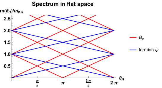
Figure 1: The mass spectrum of gauge fields $B_{\mu}^{\langle n\rangle}$ and fermion fields $\psi^{\langle n\rangle}$ in flat $M^{4}\times(S^{1}/Z_{2})$ spacetime is displayed. Level crossings in the spectrum are seen.

Next we examine $SU(2)$ GHU in the RS space whose metric is given by [14]

$$ds^{2}=e^{-2\sigma(y)}\eta_{\mu\nu}dx^{\mu}dx^{\nu}+dy^{2}$$ (2.39)

where $\eta_{\mu\nu}=\mbox{diag}(-1,+1,+1,+1)$, $\sigma(y)=\sigma(y+2L)=\sigma(-y)$ and $\sigma(y)=ky$ for $0\leq y\leq L$. It has the same topology as $M^{4}\times(S^{1}/Z_{2})$. In the fundamental region $0\leq y\leq L$ the metric can be written, in terms of the conformal coordinate $z=e^{ky}$, as

$$ds^{2}=\frac{1}{z^{2}}\bigg{(}\eta_{\mu\nu}dx^{\mu}dx^{\nu}+\frac{dz^{2}}{k^{2}}\bigg{)}\quad(1\leq z\leq z_{L}=e^{kL})~{}.$$ (2.40)

$z_{L}$ is called the warp factor of the RS space. The action in RS is

$$I_{\rm RS} =\int d^{5}x\sqrt{-\det G}\,{\cal L}_{\rm RS}~{},$$ (2.41)

$${\cal L}_{\rm RS} =-\frac{1}{2}{\rm Tr}\,F_{MN}F^{MN}+\overline{\Psi}{\cal D}(c)\Psi+\overline{\Psi}{}^{\prime}{\cal D}(c^{\prime})\Psi^{\prime}~{},$$ (2.42)

$${\cal D}(c) =\gamma^{A}{e_{A}}^{M}\bigg{(}D_{M}+\frac{1}{8}\omega_{MBC}[\gamma^{B},\gamma^{C}]\bigg{)}-c\,k\quad{\rm for}~{}1\leq z\leq z_{L}~{}.$$ (2.43)

Note ${\cal L}_{\rm RS}(x^{\mu},y)={\cal L}_{\rm RS}(x^{\mu},-y)={\cal L}_{\rm RS}(x^{\mu},y+2L)$. Fields $A_{M}$, $\Psi$ and $\Psi^{\prime}$ satisfy the same boundary conditions (2.6) as in the flat space. The dimensionless bulk mass parameter $c$ in ${\cal D}(c)$ controls the mass and wave function of fermion fields. The KK mass scale is given by

$$m_{{\rm KK}} =\frac{\pi k}{z_{L}-1}$$ (2.44)

which becomes $1/R$ in the flat spacetime limit $k\rightarrow 0$.

In the KK expansion $A_{z}^{a}(x,z)=k^{-1/2}\sum A_{z}^{a(n)}(x)h_{n}(z)$, the zero mode $A_{z}^{2(0)}$ has a wave function $h_{0}(z)=\sqrt{2/(z_{L}^{2}-1)}\,z$. In the $y$-coordinate $A_{y}^{2(0)}$ has a wave function $v_{0}(y)=ke^{ky}h_{0}(z)$ for $0\leq y\leq L$ and $v_{0}(-y)=v_{0}(y)=v_{0}(y+2L)$. The AB phase $\theta_{H}$ in (2.13) becomes

$$\theta_{H} =\frac{\langle A_{z}^{2(0)}\rangle}{f_{H}}~{},~{}~{}f_{H}=\frac{1}{g_{4}}\sqrt{\frac{2k}{L(z_{L}^{2}-1)}}~{}.$$ (2.45)

The twisted gauge [12, 13], in which $\tilde{\theta}_{H}=0$, is related to the original gauge by a large gauge transformation

$$\Omega(z) =e^{i\theta(z)\tau^{2}/2}~{},~{}~{}\theta(z)=\theta_{H}\,\frac{z_{L}^{2}-z^{2}}{z_{L}^{2}-1}~{}.$$ (2.46)

In the $y$-coordinate it is written as

$$\Omega(y) =\exp\bigg{\{}i\theta_{H}\sqrt{\frac{2}{z_{L}^{2}-1}}\int_{y}^{L}dy\,v_{0}(y)\cdot\frac{\tau^{2}}{2}\bigg{\}}.$$ (2.47)

The boundary conditions in the twisted gauge are given by (2.17).

With the boundary conditions at $z=z_{L}$ eigenmodes of $\tilde{A}_{\mu}^{1}$ and $\tilde{A}_{\mu}^{3}$ are given in the form

$$\begin{pmatrix}\tilde{A}_{\mu}^{1}\cr\tilde{A}_{\mu}^{3}\end{pmatrix} =\begin{pmatrix}\alpha S(z;\lambda)\cr\beta C(z;\lambda)\end{pmatrix}Z_{\mu}^{(\lambda)}(x)$$ (2.48)

where $S(z;\lambda)$ and $C(z;\lambda)$ are expressed in terms of Bessel functions and are given by (A.5). The boundary conditions at $z=1$ lead to a condition obtained from (2.22) by substituting $S_{\lambda}(0),C_{\lambda}(0)$ etc. by $S(1;\lambda),C(1;\lambda)$ etc. As $(CS^{\prime}-SC^{\prime})(z;\lambda)=\lambda z$, the spectrum is determined by

$$SC^{\prime}(1;\lambda_{n})+\lambda_{n}\sin^{2}\theta_{H}=0~{}.$$ (2.49)

The corresponding mass is $m_{n}=k\lambda_{n}$. We label $\{\lambda_{n}\}$ from the bottom such that $\lambda_{0}(\theta_{H})<\lambda_{1}(\theta_{H})<\lambda_{2}(\theta_{H})<\cdots$. There is no level crossing. The spectrum is periodic with a period $\pi$, and is displayed in Fig. 2.

For a fermion field $\Psi(x,z)$ it is most convenient to express its KK expansion for $\check{\Psi}(x,z)=z^{-2}\Psi(x,z)$. Note that Neumann boundary conditions at $z=(z_{0},z_{1})=(1,z_{L})$, corresponding to even parity, for left- and right-handed components are given by

$$D_{+}(c)\check{\Psi}_{L}\big{|}_{z_{j}}=0~{},~{}~{}D_{-}(c)\check{\Psi}_{R}\big{|}_{z_{j}}=0~{},~{}~{}D_{\pm}(c)=\pm\frac{d}{dz}+\frac{c}{z}~{}.$$ (2.50)

In the twisted gauge $\tilde{\check{\Psi}}$ satisfies free equations in the bulk. With the boundary conditions at $z=z_{L}$ eigenmodes of $\check{\Psi}$ are written in the form

$$\begin{pmatrix}\tilde{\check{u}}_{R}\cr\tilde{\check{d}}_{R}\end{pmatrix}(x,z) =\begin{pmatrix}\alpha_{R}C_{R}(z;\lambda,c)\cr\beta_{R}S_{R}(z;\lambda,c)\end{pmatrix}f_{\lambda,R}(x)~{},$$ (2.51)

$$\begin{pmatrix}\tilde{\check{u}}_{L}\cr\tilde{\check{d}}_{L}\end{pmatrix}(x,z) =\begin{pmatrix}\alpha_{L}S_{L}(z;\lambda,c)\cr\beta_{L}C_{L}(z;\lambda,c)\end{pmatrix}f_{\lambda,L}(x)~{},$$ (2.52)

where functions $C_{R/L}$ and $S_{R/L}$ are given in (A.14). It follows from the equations of motion that $(\alpha_{R},\beta_{R})=(\alpha_{L},\beta_{L})$. The boundary conditions at $z=1$, $D_{-}\check{u}_{R}=0$ and $\check{d}_{R}=0$, lead to

$$\begin{pmatrix}\bar{s}_{H}C_{R}(1)&\bar{c}_{H}S_{R}(1)\cr\bar{c}_{H}S_{L}(1)&-\bar{s}_{H}C_{L}(1)\end{pmatrix}\begin{pmatrix}\alpha_{R}\cr\beta_{R}\end{pmatrix}=0~{},$$ (2.53)

where $C_{R}(1)=C_{R}(1;\lambda,c)$ etc. and the relation $D_{-}(c)(C_{R},S_{R})=\lambda(S_{L},C_{L})$ has been used. As $C_{L}C_{R}-S_{L}S_{R}=1$, the spectrum is determined by

$$S_{L}S_{R}(1;\lambda_{n},c)+\sin^{2}\hbox{$\frac{1}{2}$}\theta_{H}=0~{}.$$ (2.54)

The corresponding mass is $m_{n}=k\lambda_{n}$. As in the case of the gauge field, we label $\{\lambda_{n}\}$ from the bottom such that $\lambda_{0}(\theta_{H})<\lambda_{1}(\theta_{H})<\lambda_{2}(\theta_{H})<\cdots$. There is no level crossing. The spectrum is periodic with a period $2\pi$, and is displayed in Fig. 2.

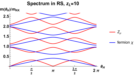
Figure 2: The mass spectrum of gauge fields $Z_{\mu}^{(n)}$ and fermion fields $\chi^{(n)}$ in the RS warped space is displayed. The warp factor is $z_{L}=10$ and the bulk mass parameter of $\Psi$ is $c=0.25$. There is no level crossing in the spectrum.

Formulas for a fermion field $\Psi^{\prime}$ are obtained in a similar manner. With the boundary conditions at $z=z_{L}$ eigenmodes of $\check{\Psi}^{\prime}$ are written in the form (2.52). The boundary conditions at $z=1$ imply that $\check{u}_{R}^{\prime}=0$ and $D_{-}\check{d}_{R}^{\prime}=0$ so that the spectrum determining equation becomes

$$S_{L}S_{R}(1;\lambda_{n},c^{\prime})+\cos^{2}\hbox{$\frac{1}{2}$}\theta_{H}=0~{}.$$ (2.55)

There appear massless modes at $\theta_{H}=\pi$.

In Fig. 2 the mass spectrum of gauge fields $Z_{\mu}^{(n)}$ and fermion fields $\chi^{(n)}$ in RS is depicted. A distinct feature is that there occurs no level crossing in the RS warped space. As the AB phase varies, the massless gauge fields $Z_{\mu}^{(0)}$ at $\theta_{H}=0$ smoothly changes to become massless gauge fields at $\theta_{H}=\pi$. The massless mode $\chi^{(0)}$ at $\theta_{H}=0$, on the other hand, becomes massive at $\theta_{H}=\pi$. Chiral fermions are transformed to vectorlike fermions by an AB phase. We shall confirm it in Section 4 by showing how gauge couplings change as $\theta_{H}$. We also stress that the spectrum in the RS space in Fig. 2 converges to the spectrum in $M^{4}\times(S^{1}/Z_{2})$ in Fig. 1 in the limit $k\rightarrow 0$ ($z_{L}\rightarrow 1$).

3 Anomaly flow in $M^{4}\times(S^{1}/Z_{2})$

4D gauge couplings of fermion fields in flat $M^{4}\times(S^{1}/Z_{2})$ spacetime are obtained by inserting the KK expansions for $A_{\mu}^{a}$ and $\Psi$ into $-ig_{A}\int d^{4}xdy\,\bar{\Psi}\gamma^{M}A_{M}\Psi$ and integrating over $y$. It is most convenient to evaluate the couplings in the original gauge as wave functions of KK modes do not depend on $\theta_{H}$ in flat spacetime.

The spectrum and KK expansion of $A_{\mu}^{2}(x,y)$ are not affected by $\theta_{H}$, and therefore

$$-\frac{ig_{A}}{2}\int_{0}^{L}dy\,A_{\mu}^{2}\big{\{}u_{R}^{\dagger}\bar{\sigma}^{\mu}d_{R}-u_{L}^{\dagger}\sigma^{\mu}d_{L}-d_{R}^{\dagger}\bar{\sigma}^{\mu}u_{R}+d_{L}^{\dagger}\sigma^{\mu}u_{L}\big{\}}$$ (3.1)

$$=-\frac{ig_{4}}{2\sqrt{2}}\sum_{n=1}^{\infty}A_{\mu}^{2(n)}\sum_{\ell=-\infty}^{\infty}\Big{\{}\psi_{R}^{\langle\ell\rangle\,\dagger}\bar{\sigma}^{\mu}\psi_{R}^{\langle\ell+n\rangle}-\psi_{R}^{\langle\ell+n\rangle\,\dagger}\bar{\sigma}^{\mu}\psi_{R}^{\langle\ell\rangle}$$ (3.2)

$$\hskip 113.81102pt-\psi_{L}^{\langle\ell\rangle\,\dagger}\sigma^{\mu}\psi_{L}^{\langle\ell+n\rangle}+\psi_{L}^{\langle\ell+n\rangle\,\dagger}\sigma^{\mu}\psi_{L}^{\langle\ell\rangle}\Big{\}}.$$ (3.3)

Here $\sigma^{\mu}=(I_{2},\vec{\sigma})$ and $\bar{\sigma}^{\mu}=(-I_{2},\vec{\sigma})$. All of $A_{\mu}^{2(n)}$ couplings do not depend on $\theta_{H}$ in the above basis. Note that the zero modes $\psi_{R}^{\langle 0\rangle}$ and $\psi_{L}^{\langle 0\rangle}$ have chiral structure in (2.35).

Couplings of $B_{\mu}^{\langle n\rangle}$ modes are evaluated similarly. By inserting the KK expansions (2.25) and (2.35), one finds

$$-\frac{ig_{A}}{2}\int_{0}^{L}dy\,\big{\{}A_{\mu}^{1}(\bar{u}\gamma^{\mu}d+\bar{d}\gamma^{\mu}u)+A_{\mu}^{3}(\bar{u}\gamma^{\mu}u-\bar{d}\gamma^{\mu}d)\big{\}}$$ (3.4)

$$=\frac{g_{4}}{2}\sum_{n=-\infty}^{\infty}B_{\mu}^{\langle n\rangle}\sum_{\ell=-\infty}^{\infty}\Big{\{}\psi_{R}^{\langle n-\ell\rangle\,\dagger}\bar{\sigma}^{\mu}\psi_{R}^{\langle\ell\rangle}+\psi_{L}^{\langle n-\ell\rangle\,\dagger}\sigma^{\mu}\psi_{L}^{\langle\ell\rangle}\Big{\}}$$ (3.5)

$$=\frac{g_{4}}{2}\sum_{n=-\infty}^{\infty}B_{\mu}^{\langle n\rangle}\sum_{\ell=-\infty}^{\infty}\bar{\psi}^{\langle n-\ell\rangle}\,i\gamma^{5}\gamma^{\mu}\psi^{\langle\ell\rangle}~{}.$$ (3.6)

In the $B_{\mu}^{\langle n\rangle}$ basis the couplings $B_{\mu}^{\langle n\rangle}\psi_{R}^{\langle m\rangle\,\dagger}\psi_{R}^{\langle\ell\rangle}$ and $B_{\mu}^{\langle n\rangle}\psi_{L}^{\langle m\rangle\,\dagger}\psi_{L}^{\langle\ell\rangle}$ take a simple form. They are $\hbox{$\frac{1}{2}$}g_{4}\,\delta_{n,m+\ell}$.

At $\theta_{H}=0$ the $n=0$ mode of $B_{\mu}^{\langle n\rangle}$ is the massless gauge field of the unbroken $U(1)$. It has axial-vector couplings $\sum_{\ell=-\infty}^{\infty}\bar{\psi}^{\langle-\ell\rangle}\,i\gamma^{5}\gamma^{\mu}\psi^{\langle\ell\rangle}$. The coupling to the $\ell=0$ modes leads to a triangle chiral anomaly of three $B_{\mu}^{\langle 0\rangle}$ legs with an anomaly coefficient $(g_{4}/2)^{3}(1+1)$, reflecting the chiral structure of $u_{R}^{(0)}$ and $d_{L}^{(0)}$. Note that off-diagonal couplings do not contribute to this anomaly. At $\theta_{H}=\pi$ the $B_{\mu}^{\langle-1\rangle}$ mode becomes the massless gauge field of the unbroken $U(1)$. It has axial-vector couplings $\sum_{\ell=-\infty}^{\infty}\bar{\psi}^{\langle-\ell-1\rangle}\,i\gamma^{5}\gamma^{\mu}\psi^{\langle\ell\rangle}$. There arises no chiral anomaly associated with three $B_{\mu}^{\langle-1\rangle}$ legs.

To investigate the structure of anomalies let us write $B_{\mu}$ couplings as

$$\frac{g_{4}}{2}\sum_{n=-\infty}^{\infty}\sum_{m=-\infty}^{\infty}\sum_{\ell=-\infty}^{\infty}B_{\mu}^{\langle n\rangle}\Big{\{}s^{R}_{nm\ell}\,\psi_{R}^{\langle m\rangle\,\dagger}\bar{\sigma}^{\mu}\psi_{R}^{\langle\ell\rangle}+s^{L}_{nm\ell}\,\psi_{L}^{\langle m\rangle\,\dagger}\sigma^{\mu}\psi_{L}^{\langle\ell\rangle}\Big{\}}$$ (3.7)

where, in the current case, $s^{R}_{nm\ell}=s^{L}_{nm\ell}=\delta_{n,m+\ell}$. The anomaly coefficient associated with three legs of $B_{\mu_{1}}^{\langle n_{1}\rangle}B_{\mu_{2}}^{\langle n_{2}\rangle}B_{\mu_{3}}^{\langle n_{3}\rangle}$ is given by

$$b_{n_{1}n_{2}n_{3}}=b_{n_{1}n_{2}n_{3}}^{R}+b_{n_{1}n_{2}n_{3}}^{L}~{},$$ (3.8)

$$b_{n_{1}n_{2}n_{3}}^{R}={\rm Tr}\,S^{R}_{n_{1}}S^{R}_{n_{2}}S^{R}_{n_{3}}~{},~{}~{}(S^{R}_{n})_{m\ell}=s^{R}_{nm\ell}~{},$$ (3.9)

$$b_{n_{1}n_{2}n_{3}}^{L}={\rm Tr}\,S^{L}_{n_{1}}S^{L}_{n_{2}}S^{L}_{n_{3}}~{},~{}~{}(S^{L}_{n})_{m\ell}=s^{L}_{nm\ell}~{}.$$ (3.10)

It follows that

$$b_{n_{1}n_{2}n_{3}}=\begin{cases}2&\hbox{for~{}}n_{1}+n_{2}+n_{3}=\hbox{even},\cr\kern 5.0pt\cr 0&\hbox{for~{}}n_{1}+n_{2}+n_{3}=\hbox{odd}.\end{cases}$$ (3.11)

Note that $b_{011},b_{200},b_{211},\cdots=2\not=0$. Anomalies arise even for massive KK excited gauge bosons in external legs. Triangle diagrams, for instance, in which fermions $\psi^{\langle 0\rangle}$, $\psi^{\langle 0\rangle}$ and $\psi^{\langle 1\rangle}$ ($\psi^{\langle 1\rangle}$, $\psi^{\langle 1\rangle}$ and $\psi^{\langle-1\rangle}$) are running, contribute to $b_{011}$ ($b_{200}$) in perturbation theory. The divergence of the current $J^{\langle n\rangle}_{\mu}$ associated with $B_{\mu}^{\langle n\rangle}$ has anomalous terms proportional to $\sum_{m\ell}b_{nm\ell}\,{\epsilon}^{\mu\nu\rho\sigma}F^{\langle m\rangle}_{\mu\nu}F^{\langle\ell\rangle}_{\rho\sigma}$ where $F^{\langle m\rangle}_{\mu\nu}=\partial_{\mu}B_{\nu}^{\langle m\rangle}-\partial_{\nu}B_{\mu}^{\langle m\rangle}$.

In the $B_{\mu}$ basis $b_{n_{1}n_{2}n_{3}}$ is $\theta_{H}$-independent. The anomaly does not seem to flow with $\theta_{H}$ in the flat space. However, the level crossing in the spectrum occurs in the flat space. The $B_{\mu}^{\langle 0\rangle}$ mode corresponds to the lowest mode for $0\leq\theta_{H}<\hbox{$\frac{1}{2}$}\pi$, but becomes the first excited KK mode for $\hbox{$\frac{1}{2}$}\pi<\theta_{H}<\pi$. In the RS space there is no level crossing. The lowest gauge field mode remains as the lowest mode for any value of $\theta_{H}$. When the AdS curvature of the RS space is very small, namely for $k\ll m_{{\rm KK}}$, the anomaly associated with three legs of the lowest gauge field must approach to $b_{nnn}$ with $n=-1$ (namely zero) for $\hbox{$\frac{1}{2}$}\pi<\theta_{H}<\pi$. In other words the anomaly must flow from 2 to 0 as $\theta_{H}$ varies from 0 to $\pi$. We are going to see in the next section how this happens.

Contributions of the $\Psi^{\prime}$ field to anomalies are evaluated in a similar manner. With the KK expansion (2.38), $B_{\mu}$ couplings are given by

$$\frac{g_{4}}{2}\sum_{n=-\infty}^{\infty}\sum_{m=-\infty}^{\infty}\sum_{\ell=-\infty}^{\infty} B_{\mu}^{\langle n\rangle}\Big{\{}s^{\prime R}_{nm\ell}\,\psi_{R}^{\prime\langle m+\frac{1}{2}\rangle\,\dagger}\bar{\sigma}^{\mu}\psi_{R}^{\prime\langle\ell+\frac{1}{2}\rangle}+s^{\prime L}_{nm\ell}\,\psi_{L}^{\prime\langle m+\frac{1}{2}\rangle\,\dagger}\sigma^{\mu}\psi_{L}^{\prime\langle\ell+\frac{1}{2}\rangle}\Big{\}}~{},$$ (3.12)

$${\rm where~{}}~{}s^{\prime R}_{nm\ell}=s^{\prime L}_{nm\ell}=\delta_{n,m+\ell+1}~{}.$$ (3.13)

The anomaly coefficient associated with $B_{\mu_{1}}^{\langle n_{1}\rangle}B_{\mu_{2}}^{\langle n_{2}\rangle}B_{\mu_{3}}^{\langle n_{3}\rangle}$ is given by formulae similar to (3.10) where all quantities are replaced by primed ones, e.g. $b_{nm\ell}\rightarrow b_{nm\ell}^{\prime}$ and $s^{R}_{nm\ell}\rightarrow s^{\prime R}_{nm\ell}$ etc. One sees that

$$b_{n_{1}n_{2}n_{3}}^{\prime}=\begin{cases}0&\hbox{for~{}}n_{1}+n_{2}+n_{3}=\hbox{even},\cr\kern 5.0pt\cr 2&\hbox{for~{}}n_{1}+n_{2}+n_{3}=\hbox{odd}.\end{cases}$$ (3.14)

4 Anomaly flow in RS

The KK expansion of gauge fields $A_{\mu}^{1,3}$ becomes

$$\begin{pmatrix}\tilde{A}_{\mu}^{1}(x,z)\cr\kern 5.0pt\cr\tilde{A}_{\mu}^{3}(x,z)\end{pmatrix} =\sqrt{k}\sum_{n=0}^{\infty}Z_{\mu}^{(n)}(x)\,{\bf h}_{n}(z)~{},$$ (4.1)

where mode functions are given by

$${\bf h}_{0}(z) =\bar{\bf h}_{0}^{a}(z)~{},$$ (4.2)

$${\bf h}_{2\ell-1}(z) =(-1)^{\ell}\begin{cases}\bar{\bf h}_{2\ell-1}^{a}(z)&{\rm for}-\frac{1}{2}\pi<\theta_{H}<\frac{1}{2}\pi\cr\bar{\bf h}_{2\ell-1}^{b}(z)&{\rm for~{}}0<\theta_{H}<\pi\cr-\bar{\bf h}_{2\ell-1}^{a}(z)&{\rm for~{}}\frac{1}{2}\pi<\theta_{H}<\frac{3}{2}\pi\cr-\bar{\bf h}_{2\ell-1}^{b}(z)&{\rm for~{}}\pi<\theta_{H}<2\pi\cr\bar{\bf h}_{2\ell-1}^{a}(z)&{\rm for~{}}\frac{3}{2}\pi<\theta_{H}<\frac{5}{2}\pi\end{cases}~{}~{}(\ell=1,2,3,\cdots),$$ (4.3)

$${\bf h}_{2\ell}(z) =(-1)^{\ell}\begin{cases}\bar{\bf h}_{2\ell}^{b}(z)&{\rm for}-\frac{1}{2}\pi<\theta_{H}<\frac{1}{2}\pi\cr-\bar{\bf h}_{2\ell}^{a}(z)&{\rm for~{}}0<\theta_{H}<\pi\cr-\bar{\bf h}_{2\ell}^{b}(z)&{\rm for~{}}\frac{1}{2}\pi<\theta_{H}<\frac{3}{2}\pi\cr\bar{\bf h}_{2\ell}^{a}(z)&{\rm for~{}}\pi<\theta_{H}<2\pi\cr\bar{\bf h}_{2\ell}^{b}(z)&{\rm for~{}}\frac{3}{2}\pi<\theta_{H}<\frac{5}{2}\pi\end{cases}~{}(\ell=1,2,3,\cdots).$$ (4.4)

Here

$$\bar{\bf h}_{n}^{a}(z)=\frac{1}{\sqrt{r^{a}_{n}}}\begin{pmatrix}-s_{H}\hat{S}(z;\lambda_{n})\cr c_{H}C(z;\lambda_{n})\end{pmatrix},$$ (4.5)

$$\bar{\bf h}_{n}^{b}(z)=\frac{1}{\sqrt{r^{b}_{n}}}\begin{pmatrix}c_{H}S(z;\lambda_{n})\cr s_{H}\check{C}(z;\lambda_{n})\end{pmatrix},$$ (4.6)

$$r_{n}=\int_{1}^{z_{L}}\frac{dz}{z}\big{\{}|h_{n}(z)|^{2}+|k_{n}(z)|^{2}\big{\}}\quad{\rm for}~{}\begin{pmatrix}h_{n}(z)\cr k_{n}(z)\end{pmatrix}.$$ (4.7)

$\hat{S}$ and $\check{C}$ are given in (A.12). The spectrum determining equation (2.49) can be written as $CS^{\prime}(1;\lambda_{n})-\lambda_{n}\cos^{2}\theta_{H}=0$. At $\theta_{H}=0$ and $\pi$, $S(1;\lambda_{n})=0$ for even $n$ and $C^{\prime}(1;\lambda_{n})=0$ for odd $n$. At $\theta_{H}=\hbox{$\frac{1}{2}$}\pi$ and $\frac{3}{2}\pi$, $S^{\prime}(1;\lambda_{n})=0$ for even $n$ and $C(1;\lambda_{n})=0$ for odd $n$. This is why the connection formulas are necessary in (4.4). The expression $\bar{\bf h}_{2\ell-1}^{a}(z)$, for instance, fails to make sense at $\theta_{H}=\frac{1}{2}\pi$ as both $\hat{S}(z;\lambda_{2\ell-1})$ and $c_{H}$ vanish there. In deriving the connection formulas, we have made use of an identity

$$\begin{pmatrix}s_{H}\hat{S}(z;\lambda_{n})\cr-c_{H}C(z;\lambda_{n})\end{pmatrix}=K\begin{pmatrix}c_{H}S(z;\lambda_{n})\cr s_{H}\check{C}(z;\lambda_{n})\end{pmatrix},$$ (4.8)

$$K=\frac{s_{H}C(1;\lambda_{n})}{c_{H}S(1;\lambda_{n})}=-\frac{c_{H}C^{\prime}(1;\lambda_{n})}{s_{H}S^{\prime}(1;\lambda_{n})}~{},$$ (4.9)

valid at $|\theta_{H}|\not=0,\hbox{$\frac{1}{2}$}\pi,\pi,\cdots$. As a consequence, $\bar{\bf h}_{2\ell-1}^{a}(z)=\bar{\bf h}_{2\ell-1}^{b}(z)$ for $0<\theta_{H}<\hbox{$\frac{1}{2}$}\pi$ and $\bar{\bf h}_{2\ell-1}^{a}(z)=-\bar{\bf h}_{2\ell-1}^{b}(z)$ for $\hbox{$\frac{1}{2}$}\pi<\theta_{H}<\pi$ in (4.4). In numerical evaluation of anomalies we have used, for instance, ${\bf h}_{2\ell-1}(z)=(-1)^{\ell}\bar{\bf h}_{2\ell-1}^{a}(z)$ for $-\frac{1}{4}\pi<\theta_{H}\leq\frac{1}{4}\pi$, $(-1)^{\ell}\bar{\bf h}_{2\ell-1}^{b}(z)$ for $\frac{1}{4}\pi<\theta_{H}\leq\frac{3}{4}\pi$ and so on. ${\bf h}_{0}(z)$ is periodic in $\theta_{H}$ with a period $2\pi$, whereas all other modes ${\bf h}_{n}(z)$ ($n\geq 1$) have a period $\pi$.

Mode functions of the fermion field $\Psi$ are found in a similar manner. In the KK expansions

$$\begin{pmatrix}\tilde{\check{u}}_{R}(x,z)\cr\kern 5.0pt\cr\tilde{\check{d}}_{R}(x,z)\end{pmatrix} =\sqrt{k}\sum_{n=0}^{\infty}\chi_{R}^{(n)}(x)\,{\bf f}_{Rn}(z)~{},$$ (4.10)

$$\begin{pmatrix}\tilde{\check{u}}_{L}(x,z)\cr\kern 5.0pt\cr\tilde{\check{d}}_{L}(x,z)\end{pmatrix} =\sqrt{k}\sum_{n=0}^{\infty}\chi_{L}^{(n)}(x)\,{\bf f}_{Ln}(z)~{},$$ (4.11)

mode functions are given, for $c>0$, by

$${\bf f}_{R,2\ell}(z) =\begin{cases}\bar{\bf f}_{R,2\ell}^{a}(z)&{\rm for~{}}-\pi<\theta_{H}<\pi\cr\bar{\bf f}_{R,2\ell}^{b}(z)&{\rm for~{}}0<\theta_{H}<2\pi\cr-\bar{\bf f}_{R,2\ell}^{a}(z)&{\rm for~{}}\pi<\theta_{H}<3\pi\cr-\bar{\bf f}_{R,2\ell}^{b}(z)&{\rm for~{}}2\pi<\theta_{H}<4\pi\cr\bar{\bf f}_{R,2\ell}^{a}(z)&{\rm for~{}}3\pi<\theta_{H}<5\pi\cr\end{cases}~{}(\ell=0,1,2,\cdots),$$ (4.12)

$${\bf f}_{R,2\ell-1}(z) =\begin{cases}\bar{\bf f}_{R,2\ell-1}^{c}(z)&{\rm for~{}}-\pi<\theta_{H}<\pi\cr\bar{\bf f}_{R,2\ell-1}^{d}(z)&{\rm for~{}}0<\theta_{H}<2\pi\cr-\bar{\bf f}_{R,2\ell-1}^{c}(z)&{\rm for~{}}\pi<\theta_{H}<3\pi\cr-\bar{\bf f}_{R,2\ell-1}^{d}(z)&{\rm for~{}}2\pi<\theta_{H}<4\pi\cr\bar{\bf f}_{R,2\ell-1}^{c}(z)&{\rm for~{}}3\pi<\theta_{H}<5\pi\cr\end{cases}~{}(\ell=1,2,3,\cdots),$$ (4.13)

and

$${\bf f}_{L0}(z) =\bar{\bf f}_{L0}^{a}(z),$$ (4.14)

$${\bf f}_{L,2\ell-1}(z) =\begin{cases}\bar{\bf f}_{L,2\ell-1}^{a}(z)&{\rm for~{}}-\pi<\theta_{H}<\pi\cr\bar{\bf f}_{L,2\ell-1}^{b}(z)&{\rm for~{}}0<\theta_{H}<2\pi\cr-\bar{\bf f}_{L,2\ell-1}^{a}(z)&{\rm for~{}}\pi<\theta_{H}<3\pi\cr-\bar{\bf f}_{L,2\ell-1}^{b}(z)&{\rm for~{}}2\pi<\theta_{H}<4\pi\cr\bar{\bf f}_{L,2\ell-1}^{a}(z)&{\rm for~{}}3\pi<\theta_{H}<5\pi\cr\end{cases}~{}(\ell=1,2,3,\cdots),$$ (4.15)

$${\bf f}_{L,2\ell}(z) =\begin{cases}\bar{\bf f}_{L,2\ell}^{c}(z)&{\rm for~{}}-\pi<\theta_{H}<\pi\cr\bar{\bf f}_{L,2\ell}^{d}(z)&{\rm for~{}}0<\theta_{H}<2\pi\cr-\bar{\bf f}_{L,2\ell}^{c}(z)&{\rm for~{}}\pi<\theta_{H}<3\pi\cr-\bar{\bf f}_{L,2\ell}^{d}(z)&{\rm for~{}}2\pi<\theta_{H}<4\pi\cr\bar{\bf f}_{L,2\ell}^{c}(z)&{\rm for~{}}3\pi<\theta_{H}<5\pi\cr\end{cases}~{}(\ell=1,2,3,\cdots),$$ (4.16)

Here

$$\bar{\bf f}_{Rn}^{a}(z)=\frac{1}{\sqrt{r^{a}_{n}}}\begin{pmatrix}\bar{c}_{H}C_{R}(z;\lambda_{n},c)\cr-\bar{s}_{H}\hat{S}_{R}(z;\lambda_{n},c)\end{pmatrix},~{}~{}\bar{\bf f}_{Rn}^{b}(z)=\frac{1}{\sqrt{r^{b}_{n}}}\begin{pmatrix}\bar{s}_{H}C_{R}(z;\lambda_{n},c)\cr\bar{c}_{H}\check{S}_{R}(z;\lambda_{n},c)\end{pmatrix},$$ (4.17)

$$\bar{\bf f}_{Rn}^{c}(z)=\frac{1}{\sqrt{r^{c}_{n}}}\begin{pmatrix}\bar{s}_{H}\hat{C}_{R}(z;\lambda_{n},c)\cr\bar{c}_{H}S_{R}(z;\lambda_{n},c)\end{pmatrix},~{}~{}\bar{\bf f}_{Rn}^{d}(z)=\frac{1}{\sqrt{r^{d}_{n}}}\begin{pmatrix}-\bar{c}_{H}\check{C}_{R}(z;\lambda_{n},c)\cr\bar{s}_{H}S_{R}(z;\lambda_{n},c)\end{pmatrix},$$ (4.18)

$$\bar{\bf f}_{Ln}^{a}(z)=\frac{1}{\sqrt{r^{a}_{n}}}\begin{pmatrix}\bar{s}_{H}\hat{S}_{L}(z;\lambda_{n},c)\cr\bar{c}_{H}C_{L}(z;\lambda_{n},c)\end{pmatrix},~{}~{}\bar{\bf f}_{Ln}^{b}(z)=\frac{1}{\sqrt{r^{b}_{n}}}\begin{pmatrix}-\bar{c}_{H}\check{S}_{L}(z;\lambda_{n},c)\cr\bar{s}_{H}C_{L}(z;\lambda_{n},c)\end{pmatrix},$$ (4.19)

$$\bar{\bf f}_{Ln}^{c}(z)=\frac{1}{\sqrt{r^{c}_{n}}}\begin{pmatrix}\bar{c}_{H}S_{L}(z;\lambda_{n},c)\cr-\bar{s}_{H}\hat{C}_{L}(z;\lambda_{n},c)\end{pmatrix},~{}~{}\bar{\bf f}_{Ln}^{d}(z)=\frac{1}{\sqrt{r^{d}_{n}}}\begin{pmatrix}\bar{s}_{H}S_{L}(z;\lambda_{n},c)\cr\bar{c}_{H}\check{C}_{L}(z;\lambda_{n},c)\end{pmatrix},$$ (4.20)

$$\hbox{where}~{}r_{n}=\int_{1}^{z_{L}}dz\big{\{}|f_{n}(z)|^{2}+|g_{n}(z)|^{2}\big{\}}\quad{\rm for}~{}\begin{pmatrix}f_{n}(z)\cr g_{n}(z)\end{pmatrix}.$$ (4.21)

Functions $\hat{S}_{R/L},\check{S}_{R/L}$ etc. are defined in (A.23). At $\theta_{H}=0$ the $n=0$ mode is massless; $\lambda_{0}=0$. Its wave function has chiral structure. $\chi_{R}^{(0)}$ is $u$-type, whereas $\chi_{L}^{(0)}$ is $d$-type. It is seen below that the $n=0$ mode becomes vectorlike as $\theta_{H}$ varies to $\pi$. At $\theta_{H}=0$, $S_{L}(1;\lambda_{n},c)=0$ for even $n$ whereas $S_{R}(1;\lambda_{n},c)=0$ for odd $n$. At $\theta_{H}=\pi$, $C_{R}(1;\lambda_{n},c)=0$ for even $n$ whereas $C_{L}(1;\lambda_{n},c)=0$ for odd $n$. This is why the connection formulas are necessary in (4.13) and (4.16). The wave function of the $\chi_{L}^{(0)}$ mode, ${\bf f}_{L0}(z)$, is periodic in $\theta_{H}$ with a period $4\pi$. Wave functions of all other modes are periodic in $\theta_{H}$ with a period $2\pi$. Wave functions for $c<0$ are tabulated in Appendix B.

The four-dimensional part of the gauge interactions for the $\Psi$ field is given by

$$g_{A}\int d^{4}x\int_{1}^{z_{L}}\frac{dz}{k}\,\Big{\{}\tilde{\check{\Psi}}_{R}^{\dagger}\bar{\sigma}^{\mu}\tilde{A}_{\mu}\tilde{\check{\Psi}}_{R}-\tilde{\check{\Psi}}_{L}^{\dagger}\sigma^{\mu}\tilde{A}_{\mu}\tilde{\check{\Psi}}_{L}\Big{\}}~{}.$$ (4.22)

To find the $Z_{\mu}^{(n)}$ couplings of fermion modes, we write

$${\bf h}_{n}(z)=\begin{pmatrix}h_{n}(z)\cr k_{n}(z)\end{pmatrix},~{}~{}{\bf f}_{Rn}(z)=\begin{pmatrix}f_{Rn}(z)\cr g_{Rn}(z)\end{pmatrix},~{}~{}{\bf f}_{Ln}(z)=\begin{pmatrix}f_{Ln}(z)\cr g_{Ln}(z)\end{pmatrix}.$$ (4.23)

By inserting the KK expansions (4.1) and (4.11) into (4.22), the $Z_{\mu}^{(n)}$ couplings of the $\chi_{n}$ fields are found to be

$$\frac{g_{4}}{2}\sum_{n=0}^{\infty}\sum_{\ell=0}^{\infty}\sum_{m=0}^{\infty}Z_{\mu}^{(n)}(x)\Big{\{}t^{R}_{n\ell m}\,\chi_{R}^{(\ell)}(x)^{\dagger}\bar{\sigma}^{\mu}\chi_{R}^{(m)}(x)+t^{L}_{n\ell m}\,\chi_{L}^{(\ell)}(x)^{\dagger}\sigma^{\mu}\chi_{L}^{(m)}(x)\Big{\}},$$ (4.24)

$$\hskip 28.45274ptt^{R}_{n\ell m}=\sqrt{kL}\int_{1}^{z_{L}}dz\,\Big{\{}h_{n}(z)\big{(}f_{R\ell}^{*}(z)g_{Rm}(z)+g_{R\ell}^{*}(z)f_{Rm}(z)\big{)}$$ (4.25)

$$\hskip 128.0374pt+k_{n}(z)\big{(}f_{R\ell}^{*}(z)f_{Rm}(z)-g_{R\ell}^{*}(z)g_{Rm}(z)\big{)}\Big{\}},$$ (4.26)

$$\hskip 28.45274ptt^{L}_{n\ell m}=-\sqrt{kL}\int_{1}^{z_{L}}dz\,\Big{\{}h_{n}(z)\big{(}f_{L\ell}^{*}(z)g_{Lm}(z)+g_{L\ell}^{*}(z)f_{Lm}(z)\big{)}$$ (4.27)

$$\hskip 128.0374pt+k_{n}(z)\big{(}f_{L\ell}^{*}(z)f_{Lm}(z)-g_{L\ell}^{*}(z)g_{Lm}(z)\big{)}\Big{\}}.$$ (4.28)

The anomaly coefficient associated with three legs of $Z_{\mu_{1}}^{(n_{1})}Z_{\mu_{2}}^{(n_{2})}Z_{\mu_{3}}^{(n_{3})}$ is given by

$$a_{n_{1}n_{2}n_{3}}=a_{n_{1}n_{2}n_{3}}^{R}+a_{n_{1}n_{2}n_{3}}^{L}~{},$$ (4.29)

$$a_{n_{1}n_{2}n_{3}}^{R}={\rm Tr}\,T^{R}_{n_{1}}T^{R}_{n_{2}}T^{R}_{n_{3}}~{},~{}~{}(T^{R}_{n})_{m\ell}=t^{R}_{nm\ell}~{},$$ (4.30)

$$a_{n_{1}n_{2}n_{3}}^{L}={\rm Tr}\,T^{L}_{n_{1}}T^{L}_{n_{2}}T^{L}_{n_{3}}~{},~{}~{}(T^{L}_{n})_{m\ell}=t^{L}_{nm\ell}~{}.$$ (4.31)

Unlike $s^{R/L}_{nm\ell}$ in the flat space, $t^{R/L}_{nm\ell}$ is $\theta_{H}$-dependent. The anomaly coefficient $a_{n_{1}n_{2}n_{3}}$ also becomes $\theta_{H}$-dependent, exhibiting the anomaly flow.

Let us first examine $a_{000}(\theta_{H})$ at $\theta_{H}=0$ and $\pi$, where the gauge field $Z_{\mu}^{(0)}$ becomes massless. At $\theta_{H}=0$, $h_{0}(z)=0$ and $k_{0}(z)=1/\sqrt{kL}$. The fermion zero mode is chiral, $g_{L0},f_{R0}\not=0$ and $g_{R0}=f_{L0}=0$. All other modes are vectorlike; $f_{R\,2\ell-1}=f_{L\,2\ell-1}=g_{R\,2\ell}=g_{L\,2\ell}=0$ for $\ell=1,2,3,\cdots$. It follows from the ortho-normality conditions that $t^{R}_{0m\ell},t^{L}_{0m\ell}=0$ for $m\not=\ell$. It is seen that $t^{R}_{000}=t^{L}_{000}=1$ and $t^{R}_{0nn}=-t^{L}_{0nn}=(-1)^{n}$ for $n\geq 1$. Hence $a_{000}(0)=2$, which is the same value as $b_{000}(0)=2$ in the flat space.

At $\theta_{H}=\pi$, $h_{0}(z)=0$ and $k_{0}(z)=-1/\sqrt{kL}$. All of the fermion modes are vectorlike; $g_{R\,2\ell}=g_{L\,2\ell}=f_{R\,2\ell+1}=f_{L\,2\ell+1}=0$ for $\ell=0,1,2,\cdots$. Further $t^{R}_{0m\ell},t^{L}_{0m\ell}=0$ for $m\not=\ell$, and $-t^{R}_{0nn}=t^{L}_{0nn}=(-1)^{n}$ for $n\geq 0$. It follows that $a_{000}(\pi)=0$, which agrees with $b_{-1,-1,-1}(\pi)=0$ in the flat space.

The $\theta_{H}$-dependence of the coupling constants $t^{R}_{000}$, $t^{L}_{000}$ and anomaly coefficients $a_{000}$, $a^{R}_{000}$, $a^{L}_{000}$ is displayed in Figs. 3 and 4 for $z_{L}=10$ and $c=0.25$. All of them smoothly changes as $\theta_{H}$. The coupling constants of the fermion zero modes are maximally chiral at $\theta_{H}=0$, but become purely vectorlike at $\theta_{H}=\pi$. The anomaly is exactly cancelled among the right-handed and left-handed components at $\theta_{H}=\pi$. We note that for the anomaly coefficient $a_{n_{1}n_{2}n_{3}}$ off-diagonal gauge couplings $t^{R/L}_{nm\ell}$ also contribute in (4.31). In the previous section we have seen that in the flat space off-diagonal gauge couplings $s^{R/L}_{nm\ell}=\delta_{n,m+\ell}$ are important to $b_{n_{1}n_{2}n_{3}}$. In the RS space the couplings $t^{R/L}_{nm\ell}(\theta_{H})$ are more involved, giving rise to the nontrivial $\theta_{H}$-dependence of $a_{nm\ell}$.

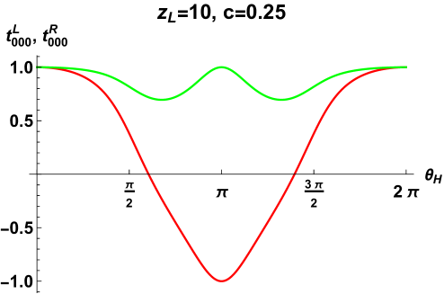
Figure 3: The coupling constants $t^{R}_{000}(\theta_{H})$ (red) and $t^{L}_{000}(\theta_{H})$ (green) in (4.28) are displayed for the warp factor $z_{L}=10$ and the bulk mass parameter $c=0.25$.

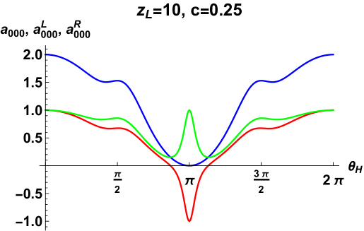
Figure 4: The anomaly coefficients $a_{000}(\theta_{H})$ (blue), $a^{R}_{000}(\theta_{H})$ (red) and $a^{L}_{000}(\theta_{H})$ (green) in (4.31) are displayed for the warp factor $z_{L}=10$ and the bulk mass parameter $c=0.25$.

Anomalies appear for various combinations of external gauge fields. In Fig. 5 anomalies $a_{111}$, $a_{222}$, $a_{001}$, and $a_{002}$ are displayed. In the RS space gauge couplings of the first excited gauge boson $Z_{\mu}^{(1)}$ to fermions become larger. Anomaly coefficients associated with $Z_{\mu}^{(1)}$ become larger as the warp factor $z_{L}$ becomes larger. Each coefficient has nontrivial $\theta_{H}$-dependence.

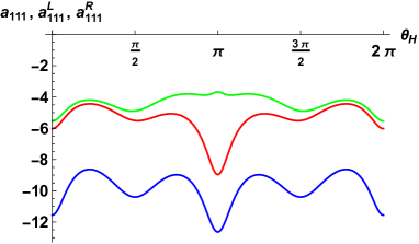
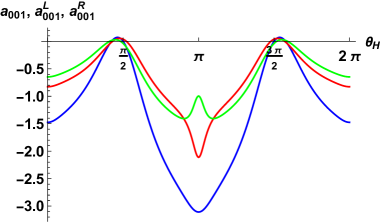
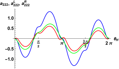
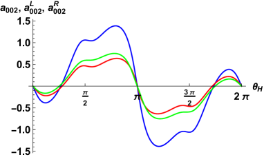
Figure 5: The anomaly coefficients $a_{111}(\theta_{H})$, $a_{001}(\theta_{H})$, $a_{222}(\theta_{H})$, $a_{002}(\theta_{H})$ in (4.31) are displayed for the warp factor $z_{L}=10$ and the bulk mass parameter $c=0.25$. Blue, red, and green lines correspond to $a_{n\ell m}$, $a_{n\ell m}^{R}$, and $a_{n\ell m}^{L}$, respectively.

The anomaly coefficient $a_{n_{1}n_{2}n_{3}}(\theta_{H})$ depends on the warp factor $z_{L}$ and the bulk mass parameter $c$ as well. The couplings $t_{000}^{R}$ and $t_{000}^{L}$ and the anomaly coefficients $a_{000}$, $a_{000}^{R}$ and $a_{000}^{L}$ for $c=0.8$ and $z_{L}=10$ are displayed in Fig. 6. The couplings of right-handed and left-handed fermions exhibit large $c$-dependence. It is seen, however, that the total anomaly coefficient $a_{000}(\theta_{H})$ is independent of $c$, being universal. In the numerical evaluation of anomalies we have incorporated contributions of fermions $\chi^{(n)}$ ($n=0,\cdots,n_{\rm max}$). In Fig. 7, $\Delta a_{000}(\theta_{H})=a_{000}(\theta_{H})_{c=0.25}-a_{000}(\theta_{H})_{c=0.8}$ is plotted with $n_{\rm max}=6,10$ and 14 for $z_{L}=10$. As $n_{\rm max}$ is increased, the difference $\Delta a_{000}(\theta_{H})$ diminishes, approaching to zero. The maximum of $|\Delta a_{000}(\theta_{H})|$ is about 0.000153 at $\theta_{H}=\frac{7}{20}\pi$ and $\frac{33}{20}\pi$ for $n_{\rm max}=14$. It is expected that $a_{000}(\theta_{H})$ becomes $c$-independent in the $n_{\rm max}\rightarrow\infty$ limit. We stress that the $c$-independence of $a_{n\ell m}(\theta_{H})$ is highly nontrivial as the gauge couplings $t_{n\ell m}^{R/L}$ depend on $c$.

For negative $c$ the role of left-handed and right-handed fermions are interchanged. In other words $t_{n\ell m}^{R}|_{-c}=t_{n\ell m}^{L}|_{c}$ and $a_{n\ell m}^{R}|_{-c}=a_{n\ell m}^{L}|_{c}$, and therefore $a_{n\ell m}(\theta_{H})_{-c}=a_{n\ell m}(\theta_{H})_{c}$.

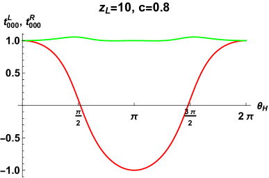
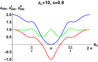
Figure 6: Left: The couplings $t_{000}^{L}$ (green) and $t_{000}^{R}$ (red). Right: The anomaly coefficients $a_{000}$ (blue), $a_{000}^{L}$ (green) and $a_{000}^{R}$ (red). Both plots are for $z_{L}=10$ and $c=0.8$. $a_{000}(\theta_{H})$ shows little dependence on $c$.

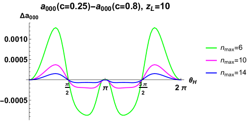
Figure 7: The dependence of the anomaly coefficient $a_{000}(\theta_{H})$ on the bulk mass parameter $c$. $a_{000}(\theta_{H})_{c=0.25}-a_{000}(\theta_{H})_{c=0.8}$ for $z_{L}=10$ evaluated by taking account of fermion modes $\chi^{(n)}$ ($n=0,\cdots,n_{\rm max}$) is shown for $n_{\rm max}=6$ (green), 10 (magenta) and 14 (blue). The result indicates $a_{000}(\theta_{H})$ becomes $c$-independent as $n_{\rm max}\rightarrow\infty$.

The $z_{L}$-dependence is investigated similarly. For large $z_{L}=e^{kL}\gg 1$ the qualitative behavior does not change very much. In Fig. 8 the couplings $t_{000}^{R}$ and $t_{000}^{L}$ and the anomaly coefficients $a_{000}$, $a_{000}^{R}$ and $a_{000}^{L}$ for $z_{L}=10^{5}$ and $c=0.25$ are displayed. Compared to the case of $z_{L}=10$ and $c=0.25$, the behavior of the anomaly coefficients becomes milder.

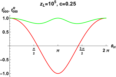
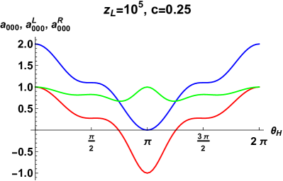
Figure 8: Left: The couplings $t_{000}^{L}$ (green) and $t_{000}^{R}$ (red). Right: The anomaly coefficients $a_{000}$ (blue), $a_{000}^{L}$ (green) and $a_{000}^{R}$ (red). Both plots are for $z_{L}=10^{5}$ and $c=0.25$.

The flat space limit, $k/m_{{\rm KK}}=(z_{L}-1)/\pi\rightarrow 0$, exhibits singular behavior. In the flat space, $M^{4}\times(S^{1}/Z_{2})$, anomaly coefficients $b_{n\ell m}(\theta_{H})$ are constant. It implies that except at the points of level crossings, $\theta_{H}=0,\pm\hbox{$\frac{1}{2}$}\pi,\pm\pi$, $a_{n\ell m}$ must approach to a constant value in the flat space limit, and therefore must show step-function type behavior. In Fig. 9 the anomaly coefficients $a_{000}(\theta_{H})$, $a_{222}(\theta_{H})$ and $a_{012}(\theta_{H})$ with $c=0.25$ are plotted for various values of $z_{L}$. It is seen that all of them approach to step functions with singularities at $\theta_{H}=0,\hbox{$\frac{1}{2}$}\pi,\pi$ or $\frac{3}{2}\pi$ as $z_{L}\rightarrow 1$.

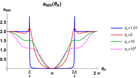
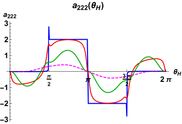
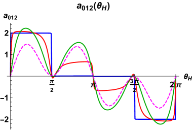
Figure 9: The anomaly coefficients $a_{000}(\theta_{H})$, $a_{222}(\theta_{H})$ and $a_{012}(\theta_{H})$ with $c=0.25$ are displayed for $z_{L}=1.01,2,10$ and $10^{5}$. The flat space limit corresponds to $k\rightarrow 0$ and $z_{L}\rightarrow 1$.

At this juncture it is appropriate to look at the correspondence between $B_{\mu}^{\langle n\rangle}$ and $Z_{\mu}^{(n)}$ in the flat space limit, which can be found from the mass spectra displayed in Fig. 1 and Fig. 2, the mode functions of $B_{\mu}^{\langle n\rangle}$ in (2.24), and the mode functions of $Z_{\mu}^{(n)}$ in (4.4). The result for $Z_{\mu}^{(n)}$ ($n=0,1,2,3$) is tabulated in Table 1. With the use of the relationships in Table 1, the anomaly coefficients in the flat space limit are easily found. For instance,

$$\lim_{k\rightarrow 0}a_{000}(\theta_{H}) =\begin{cases}b_{000}\cr\frac{1}{2\sqrt{2}}(b_{000}+b_{-1-1-1}+3b_{0-1-1}+3b_{00-1})\cr b_{-1-1-1}\cr\frac{1}{2\sqrt{2}}(b_{-1-1-1}+b_{-2-2-2}+3b_{-1-2-2}+3b_{-1-1-2})\cr b_{-2-2-2}\end{cases}$$ (4.32)

$$=\begin{cases}2&{\rm for~{}}0\leq\theta_{H}<\frac{1}{2}\pi\cr 2\sqrt{2}&{\rm for~{}}\theta_{H}=\frac{1}{2}\pi\cr 0&{\rm for~{}}\frac{1}{2}\pi<\theta_{H}<\frac{3}{2}\pi\cr 2\sqrt{2}&{\rm for~{}}\theta_{H}=\frac{3}{2}\pi\cr 2&{\rm for~{}}\frac{3}{2}\pi<\theta_{H}\leq 2\pi\end{cases}~{}.$$ (4.33)

In Table 2, some of the anomaly coefficients in the flat space limit are tabulated.

$\theta_{H}$	$Z^{(0)}$	$Z^{(1)}$	$Z^{(2)}$	$Z^{(3)}$
$0$	$B^{\langle 0\rangle}$	$\frac{1}{\sqrt{2}}(B^{\langle 1\rangle}+B^{\langle-1\rangle})$	$\frac{1}{\sqrt{2}}(B^{\langle 1\rangle}-B^{\langle-1\rangle})$	$\frac{1}{\sqrt{2}}(B^{\langle 2\rangle}+B^{\langle-2\rangle})$
$(0,\frac{1}{2}\pi)$	$B^{\langle 0\rangle}$	$B^{\langle-1\rangle}$	$B^{\langle 1\rangle}$	$B^{\langle-2\rangle}$
$\frac{1}{2}\pi$	$\frac{1}{\sqrt{2}}(B^{\langle-1\rangle}+B^{\langle 0\rangle})$	$\frac{1}{\sqrt{2}}(B^{\langle-1\rangle}-B^{\langle 0\rangle})$	$\frac{1}{\sqrt{2}}(B^{\langle-2\rangle}+B^{\langle 1\rangle})$	$\frac{1}{\sqrt{2}}(B^{\langle-2\rangle}-B^{\langle 1\rangle})$
$(\frac{1}{2}\pi,\pi)$	$B^{\langle-1\rangle}$	$-B^{\langle 0\rangle}$	$B^{\langle-2\rangle}$	$-B^{\langle 1\rangle}$
$\pi$	$B^{\langle-1\rangle}$	$\frac{-1}{\sqrt{2}}(B^{\langle-2\rangle}+B^{\langle 0\rangle})$	$\frac{1}{\sqrt{2}}(B^{\langle-2\rangle}-B^{\langle 0\rangle})$	$\frac{-1}{\sqrt{2}}(B^{\langle-3\rangle}+B^{\langle 1\rangle})$
$(\pi,\frac{3}{2}\pi)$	$B^{\langle-1\rangle}$	$-B^{\langle-2\rangle}$	$-B^{\langle 0\rangle}$	$-B^{\langle-3\rangle}$
$\frac{3}{2}\pi$	$\frac{1}{\sqrt{2}}(B^{\langle-1\rangle}+B^{\langle-2\rangle})$	$\frac{1}{\sqrt{2}}(B^{\langle-1\rangle}-B^{\langle-2\rangle})$	$\frac{-1}{\sqrt{2}}(B^{\langle 0\rangle}+B^{\langle-3\rangle})$	$\frac{1}{\sqrt{2}}(B^{\langle 0\rangle}-B^{\langle-3\rangle})$
$(\frac{3}{2}\pi,2\pi)$	$B^{\langle-2\rangle}$	$B^{\langle-1\rangle}$	$-B^{\langle-3\rangle}$	$B^{\langle 0\rangle}$
$2\pi$	$B^{\langle-2\rangle}$	$\frac{1}{\sqrt{2}}(B^{\langle-1\rangle}+B^{\langle-3\rangle})$	$\frac{1}{\sqrt{2}}(B^{\langle-1\rangle}-B^{\langle-3\rangle})$	$\frac{1}{\sqrt{2}}(B^{\langle 0\rangle}+B^{\langle-4\rangle})$
$(2\pi,\frac{5}{2}\pi)$	$B^{\langle-2\rangle}$	$B^{\langle-3\rangle}$	$B^{\langle-1\rangle}$	$B^{\langle-4\rangle}$

Table 1: The correspondence between $B_{\mu}^{\langle n\rangle}$ and $Z_{\mu}^{(n)}$ in the flat space limit is shown.

$\theta_{H}$	$a_{000}$	$a_{111}$	$a_{222}$	$a_{001}$	$a_{011}$	$a_{002}$	$a_{022}$	$a_{012}$
$0$	2	0	0	0	4	0	0	0
$(0,\frac{1}{2}\pi)$	2	0	0	0	2	0	2	2
$\frac{1}{2}\pi$	$2\sqrt{2}$	$-2\sqrt{2}$	$2\sqrt{2}$	0	0	$2\sqrt{2}$	$2\sqrt{2}$	0
$(\frac{1}{2}\pi,\pi)$	0	$-2$	2	$-2$	0	2	0	0
$\pi$	0	$-4\sqrt{2}$	0	$-2\sqrt{2}$	0	0	0	0
$(\pi,\frac{3}{2}\pi)$	0	$-2$	$-2$	$-2$	0	$-2$	0	0
$\frac{3}{2}\pi$	$2\sqrt{2}$	$-2\sqrt{2}$	$-2\sqrt{2}$	0	0	$-2\sqrt{2}$	$2\sqrt{2}$	0
$(\frac{3}{2}\pi,2\pi)$	2	0	0	0	2	0	2	$-2$
$2\pi$	2	0	0	0	4	0	0	0

Table 2: The anomaly coefficients $a_{n\ell m}(\theta_{H})$ due to the $\Psi$ field in the flat space limit are shown. Singular behavior is observed at $\theta_{H}=0,\frac{1}{2}\pi,\pi$ and $\frac{3}{2}\pi$.

The behavior of the anomaly coefficients for $z_{L}=1.01$ depicted in Fig.  9 is understood from the limiting values tabulated in Table 2. In the RS space the anomaly coefficients $a_{n\ell m}(\theta_{H})$ smoothly vary in $\theta_{H}$. In the flat space limit, however, they exhibit singular behavior at $\theta_{H}=0,\frac{1}{2}\pi,\pi$ and $\frac{3}{2}\pi$. This phenomenon is tightly connected with the emergence of the level crossings in the mass spectrum of the gauge and fermion fields at those points.

Contributions of the $\Psi^{\prime}$ field to anomalies are evaluated in a similar manner. The spectrum of the $\Psi^{\prime}$ field is given by (2.55). Mode functions ${\bf f}_{Rn}^{\prime}(z)$ and ${\bf f}_{Ln}^{\prime}(z)$ are obtained from ${\bf f}_{Rn}(z)$ and ${\bf f}_{Ln}(z)$ in (4.13) and (4.16) by making a shift $\theta_{H}\rightarrow\theta_{H}+\pi$. For instance, ${\bf f}_{R,2\ell}^{\prime}(z)$ is given by ${\bar{\bf f}}_{R,2\ell}^{\prime a}(z)={\bar{\bf f}}_{R,2\ell}^{b}(z)|_{\theta_{H}\rightarrow\theta_{H}+\pi}$ for $-\pi<\theta_{H}<\pi$ and ${\bar{\bf f}}_{R,2\ell}^{\prime b}(z)=-{\bar{\bf f}}_{R,2\ell}^{a}(z)|_{\theta_{H}\rightarrow\theta_{H}+\pi}$ for $\pi<\theta_{H}<2\pi$. As in the case of the anomaly coefficients $a_{nm\ell}$ coming from the $\Psi$ field, the anomaly coefficients $a_{nm\ell}^{\prime}$ coming from the $\Psi^{\prime}$ field exhibit singular behavior in the flat space limit. In Table 3, some of the anomaly coefficients $a_{nm\ell}^{\prime}$ in the flat space limit are tabulated.

$\theta_{H}$	$a_{000}^{\prime}$	$a_{111}^{\prime}$	$a_{222}^{\prime}$	$a_{001}^{\prime}$	$a_{011}^{\prime}$	$a_{002}^{\prime}$	$a_{022}^{\prime}$	$a_{012}^{\prime}$
$0$	0	$4\sqrt{2}$	0	$2\sqrt{2}$	0	0	0	0
$(0,\frac{1}{2}\pi)$	0	$2$	$2$	$2$	0	$2$	0	0
$\frac{1}{2}\pi$	$2\sqrt{2}$	$2\sqrt{2}$	$2\sqrt{2}$	0	0	$2\sqrt{2}$	$2\sqrt{2}$	0
$(\frac{1}{2}\pi,\pi)$	2	0	0	0	2	0	2	$-2$
$\pi$	2	0	0	0	4	0	0	0
$(\pi,\frac{3}{2}\pi)$	2	0	0	0	2	0	2	2
$\frac{3}{2}\pi$	$2\sqrt{2}$	$2\sqrt{2}$	$-2\sqrt{2}$	0	0	$-2\sqrt{2}$	$2\sqrt{2}$	0
$(\frac{3}{2}\pi,2\pi)$	0	$2$	$-2$	$2$	0	$-2$	0	0
$2\pi$	0	$4\sqrt{2}$	0	$2\sqrt{2}$	0	0	0	0

Table 3: The anomaly coefficients $a_{n\ell m}^{\prime}(\theta_{H})$ due to the $\Psi^{\prime}$ field in the flat space limit are shown. Singular behavior is observed at $\theta_{H}=0,\frac{1}{2}\pi,\pi$ and $\frac{3}{2}\pi$. $a_{n\ell m}^{\prime}(\theta_{H})$ is related to $a_{n\ell m}(\theta_{H})$ in Table 2 by $a_{n\ell m}^{\prime}(\theta_{H})=a_{n\ell m}(\theta_{H}+\pi)$ or $-a_{n\ell m}(\theta_{H}+\pi)$.

5 Summary and discussion

In this paper we have shown that chiral triangle anomalies smoothly flow in the scheme of $SU(2)$ GHU models in the RS space as the AB phase $\theta_{H}$ in the fifth dimension varies. Zero modes of $SU(2)$ doublet fermions $\Psi$ have chiral gauge couplings at $\theta_{H}=0$. Those gauge couplings smoothly change as $\theta_{H}$, and they become vectorlike at $\theta_{H}=\pi$. Although everything changes smoothly in the RS space, the flat space limit becomes singular at $\theta_{H}=0,\frac{1}{2}\pi,\pi$ and $\frac{3}{2}\pi$ where the level crossings in the mass spectrum occur in the flat $M^{4}\times(S^{1}/Z_{2})$ spacetime.

The anomaly coefficients $a^{R}_{n\ell m}(\theta_{H})$ and $a^{L}_{n\ell m}(\theta_{H})$ in the RS space depend on the warp factor $z_{L}$ and the bulk mass parameter $c$ of the fermion field. We have confirmed by numerical evaluation that the total anomaly coefficients $a_{n\ell m}(\theta_{H})=a^{R}_{n\ell m}(\theta_{H})+a^{L}_{n\ell m}(\theta_{H})$ are independent of the value of $c$. This may have profound implications for realistic GHU models in the RS space. In the $SO(5)\times U(1)\times SU(3)$ GHU [15, 16, 17], for instance, quark-lepton multiplets are introduced such that all gauge anomalies are cancelled at $\theta_{H}=0$. Each quark or lepton multiplet has its own bulk mass parameter $c$. In the vacuum $\theta_{H}\not=0$ and the electroweak symmetry is dynamically broken. Typically $\theta_{H}\sim 0.1$ and $z_{L}=10^{5}\sim 10^{10}$. Gauge couplings of right- and left-handed quark or lepton change slightly at $\theta_{H}\not=0$, depending on $c$. The universality of $a_{n\ell m}(\theta_{H})$ implies that all gauge anomalies remain cancelled even at $\theta_{H}\not=0$.[18, 19]

Anomalies flow by an AB phase. It is known that anomalies in four dimensions are related to global topology of the space through the index theorem.[20, 21] It is challenging to understand the anomaly flow by an AB phase from the viewpoint of the index theorem.[22, 23] Gauge theory in the RS space or in the flat $M^{4}\times(S^{1}/Z_{2})$ spacetime can be formulated as gauge theory on an interval $(0\leq y\leq L)$ in the fifth dimension with a special class of orbifold boundary conditions at $y=0$ and $L$. In the twisted gauge in GHU the AB phase $\theta_{H}$ appears as a phase parameter specifying orbifold boundary conditions. Anomaly and the index theorem in orbifold gauge theory with nonvanishing $\theta_{H}$ have not been well understood so far. To elucidate the anomaly flow by $\theta_{H}$ the RS space will provide a powerful tool as there occurs no level crossing in the mass spectrum and anomaly smoothly changes as $\theta_{H}$, quite in contrast to the behavior in the flat space.

Appendix A Basis functions

Wave functions of gauge fields and fermions are expressed in terms of the following basis functions. For gauge fields we introduce

$$C(z;\lambda) =\frac{\pi}{2}\lambda zz_{L}F_{1,0}(\lambda z,\lambda z_{L})~{},$$ (A.1)

$$S(z;\lambda) =-\frac{\pi}{2}\lambda zF_{1,1}(\lambda z,\lambda z_{L})~{},$$ (A.2)

$$C^{\prime}(z;\lambda) =\frac{\pi}{2}\lambda^{2}zz_{L}F_{0,0}(\lambda z,\lambda z_{L})~{},$$ (A.3)

$$S^{\prime}(z;\lambda) =-\frac{\pi}{2}\lambda^{2}zF_{0,1}(\lambda z,\lambda z_{L})~{},$$ (A.4)

$$F_{\alpha,\beta}(u,v) \equiv J_{\alpha}(u)Y_{\beta}(v)-Y_{\alpha}(u)J_{\beta}(v)~{},$$ (A.5)

where $J_{\alpha}(u)$ and $Y_{\alpha}(u)$ are Bessel functions of the first and second kind. They satisfy

$$-z\frac{d}{dz}\frac{1}{z}\frac{d}{dz}\begin{pmatrix}C\cr S\end{pmatrix}=\lambda^{2}\begin{pmatrix}C\cr S\end{pmatrix}~{},$$ (A.6)

$$C(z_{L};\lambda)=z_{L}~{},~{}~{}C^{\prime}(z_{L};\lambda)=0~{},$$ (A.7)

$$S(z_{L};\lambda)=0~{},~{}~{}S^{\prime}(z_{L};\lambda)=\lambda~{},$$ (A.8)

$$CS^{\prime}-SC^{\prime}=\lambda z~{}.$$ (A.9)

To express wave functions of KK modes of gauge fields, we make use of

$$\hat{S}(z;\lambda)=N_{0}(\lambda)S(z;\lambda)~{},~{}~{}\hat{C}(z;\lambda)=N_{0}(\lambda)^{-1}C(z;\lambda)~{},$$ (A.10)

$$\check{S}(z;\lambda)=N_{1}(\lambda)S(z;\lambda)~{},~{}~{}\check{C}(z;\lambda)=N_{1}(\lambda)^{-1}C(z;\lambda)~{},$$ (A.11)

$$\qquad N_{0}(\lambda)=\frac{C(1;\lambda)}{S(1;\lambda)}~{},~{}~{}N_{1}(\lambda)=\frac{C^{\prime}(1;\lambda)}{S^{\prime}(1;\lambda)}~{}.$$ (A.12)

For fermion fields with a bulk mass parameter $c$, we define

$$\begin{pmatrix}C_{L}\cr S_{L}\end{pmatrix}(z;\lambda,c) =\pm\frac{\pi}{2}\lambda\sqrt{zz_{L}}F_{c+\frac{1}{2},c\mp\frac{1}{2}}(\lambda z,\lambda z_{L})~{},$$ (A.13)

$$\begin{pmatrix}C_{R}\cr S_{R}\end{pmatrix}(z;\lambda,c) =\mp\frac{\pi}{2}\lambda\sqrt{zz_{L}}F_{c-\frac{1}{2},c\pm\frac{1}{2}}(\lambda z,\lambda z_{L})~{}.$$ (A.14)

These functions satisfy

$$D_{+}(c)\begin{pmatrix}C_{L}\cr S_{L}\end{pmatrix}=\lambda\begin{pmatrix}S_{R}\cr C_{R}\end{pmatrix},$$ (A.15)

$$D_{-}(c)\begin{pmatrix}C_{R}\cr S_{R}\end{pmatrix}=\lambda\begin{pmatrix}S_{L}\cr C_{L}\end{pmatrix},~{}~{}D_{\pm}(c)=\pm\frac{d}{dz}+\frac{c}{z}~{},$$ (A.16)

$$C_{R}=C_{L}=1~{},~{}~{}S_{R}=S_{L}=0\quad{\rm at~{}}z=z_{L}~{},$$ (A.17)

$$C_{L}C_{R}-S_{L}S_{R}=1~{}.$$ (A.18)

Also $C_{L}(z;\lambda,-c)=C_{R}(z;\lambda,c)$ and $S_{L}(z;\lambda,-c)=-S_{R}(z;\lambda,c)$ hold. To express wave functions of KK modes of fermion fields, we make use of

$$\hat{S}_{L}(z;\lambda,c)=N_{L}(\lambda,c)S_{L}(z;\lambda,c)~{},~{}~{}\hat{C}_{L}(z;\lambda,c)=N_{R}(\lambda,c)C_{L}(z;\lambda,c)~{},$$ (A.19)

$$\hat{S}_{R}(z;\lambda,c)=N_{R}(\lambda,c)S_{R}(z;\lambda,c)~{},~{}~{}\hat{C}_{R}(z;\lambda,c)=N_{L}(\lambda,c)C_{R}(z;\lambda,c)~{},$$ (A.20)

$$\check{S}_{L}(z;\lambda,c)=N_{R}(\lambda,c)^{-1}S_{L}(z;\lambda,c)~{},~{}~{}\check{C}_{L}(z;\lambda,c)=N_{L}(\lambda,c)^{-1}C_{L}(z;\lambda,c)~{},$$ (A.21)

$$\check{S}_{R}(z;\lambda,c)=N_{L}(\lambda,c)^{-1}S_{R}(z;\lambda,c)~{},~{}~{}\check{C}_{R}(z;\lambda,c)=N_{R}(\lambda,c)^{-1}C_{R}(z;\lambda,c)~{},$$ (A.22)

$$\qquad N_{L}(\lambda,c)=\frac{C_{L}(1;\lambda,c)}{S_{L}(1;\lambda,c)}~{},~{}~{}N_{R}(\lambda,c)=\frac{C_{R}(1;\lambda,c)}{S_{R}(1;\lambda,c)}~{}.$$ (A.23)

Appendix B Mode functions of fermion fields with $c<0$

When the bulk mass parameter $c$ of a fermion field $\Psi(x,z)$ is negative, the roles of right-handed and left-handed components are interchanged compared with those of a field with a positive $c$. In the KK expansions (4.11) mode functions ${\bf f}_{Rn}(z)$ and ${\bf f}_{Ln}(z)$ are given, for $c<0$, by

$${\bf f}_{R0}(z) =\bar{\bf f}_{R0}^{a}(z),$$ (B.1)

$${\bf f}_{R,2\ell-1}(z) =\begin{cases}\bar{\bf f}_{R,2\ell-1}^{a}(z)&{\rm for~{}}-\pi<\theta_{H}<\pi\cr\bar{\bf f}_{R,2\ell-1}^{b}(z)&{\rm for~{}}0<\theta_{H}<2\pi\cr-\bar{\bf f}_{R,2\ell-1}^{a}(z)&{\rm for~{}}\pi<\theta_{H}<3\pi\cr-\bar{\bf f}_{R,2\ell-1}^{b}(z)&{\rm for~{}}2\pi<\theta_{H}<4\pi\cr\bar{\bf f}_{R,2\ell-1}^{a}(z)&{\rm for~{}}3\pi<\theta_{H}<5\pi\cr\end{cases}~{}(\ell=1,2,3,\cdots),$$ (B.2)

$${\bf f}_{R,2\ell}(z) =\begin{cases}\bar{\bf f}_{R,2\ell}^{c}(z)&{\rm for~{}}-\pi<\theta_{H}<\pi\cr\bar{\bf f}_{R,2\ell}^{d}(z)&{\rm for~{}}0<\theta_{H}<2\pi\cr-\bar{\bf f}_{R,2\ell}^{c}(z)&{\rm for~{}}\pi<\theta_{H}<3\pi\cr-\bar{\bf f}_{R,2\ell}^{d}(z)&{\rm for~{}}2\pi<\theta_{H}<4\pi\cr\bar{\bf f}_{R,2\ell}^{c}(z)&{\rm for~{}}3\pi<\theta_{H}<5\pi\cr\end{cases}~{}(\ell=1,2,3,\cdots),$$ (B.3)

and

$${\bf f}_{L,2\ell}(z) =\begin{cases}\bar{\bf f}_{L,2\ell}^{a}(z)&{\rm for~{}}-\pi<\theta_{H}<\pi\cr\bar{\bf f}_{L,2\ell}^{b}(z)&{\rm for~{}}0<\theta_{H}<2\pi\cr-\bar{\bf f}_{L,2\ell}^{a}(z)&{\rm for~{}}\pi<\theta_{H}<3\pi\cr-\bar{\bf f}_{L,2\ell}^{b}(z)&{\rm for~{}}2\pi<\theta_{H}<4\pi\cr\bar{\bf f}_{L,2\ell}^{a}(z)&{\rm for~{}}3\pi<\theta_{H}<5\pi\cr\end{cases}~{}(\ell=0,1,2,\cdots),$$ (B.4)

$${\bf f}_{L,2\ell-1}(z) =\begin{cases}\bar{\bf f}_{L,2\ell-1}^{c}(z)&{\rm for~{}}-\pi<\theta_{H}<\pi\cr\bar{\bf f}_{L,2\ell-1}^{d}(z)&{\rm for~{}}0<\theta_{H}<2\pi\cr-\bar{\bf f}_{L,2\ell-1}^{c}(z)&{\rm for~{}}\pi<\theta_{H}<3\pi\cr-\bar{\bf f}_{L,2\ell-1}^{d}(z)&{\rm for~{}}2\pi<\theta_{H}<4\pi\cr\bar{\bf f}_{L,2\ell-1}^{c}(z)&{\rm for~{}}3\pi<\theta_{H}<5\pi\cr\end{cases}~{}(\ell=1,2,3,\cdots).$$ (B.5)

Here $\bar{\bf f}_{Rn}^{a}(z)$, $\bar{\bf f}_{Rn}^{b}(z)$ etc. are given in (4.21).

References