Fixed Points in Supersymmetric Extensions of the Standard Model

Abstract

We search for weakly interacting fixed points in extensions of the minimally supersymmetric standard model (MSSM). Necessary conditions lead to three distinct classes of anomaly-free extensions involving either new quark singlets, new quark doublets, or a fourth generation. While interacting fixed points arise prolifically in asymptotically free theories, their existence is significantly constrained as soon as some of the non-abelian gauge sectors are infrared free. Performing a scan over $\sim 200$k different MSSM extensions using matter field multiplicities and the number of superpotential couplings as free parameters, we find mostly infrared conformal fixed points, and a small subset with ultraviolet ones. All settings predict low-scale supersymmetry-breaking and a violation of $R$-parity. Despite of residual interactions, the running of couplings out of asymptotically safe fixed points is logarithmic as in asymptotic freedom. Some fixed points can be matched to the Standard Model though the matching scale comes out too low. Prospects for higher matching scales and asymptotic safety beyond the MSSM are indicated.

I Introduction

Supersymmetry (SUSY) continues to be an important driver for particle physics and model building. Over the past decades, a plethora of supersymmetric extensions have been constructed and scrutinised both in theory and experiment as appealing templates for the next Standard Model (SM). Thus far, however, the LHC has returned null results ParticleDataGroup:2020ssz , thereby strengthening earlier understandings from LEP Barbieri:2000gf . Clearly, this state of affairs requires to rethink model building paradigms and incentives, as well as vanilla parameter spaces for masses and couplings in the ongoing quest for SUSY at colliders and beyond, e.g. Arkani-Hamed:2004ymt ; Baer:2020kwz .

New directions for model building have arisen recently from the theory frontier thanks to the discovery of particle theories with interacting ultraviolet (UV) fixed points Bond:2016dvk ; Bond:2018oco ; Litim:2014uca ; Bond:2017tbw ; Bond:2019npq ; Bond:2021tgu ; Bond:2017lnq ; Bond:2017suy . UV fixed points are key for a fundamental definition of quantum field theory, in particular when asymptotic freedom is absent Bond:2016dvk ; Bond:2018oco . Without supersymmetry, they have by now been observed abundantly in settings with simple Litim:2014uca ; Bond:2017tbw ; Bond:2019npq ; Bond:2021tgu or semi-simple Bond:2017lnq gauge groups. Yukawa interactions are key for theories to become “asymptotically safe” (a term originally coined for the field-theoretic UV completion of gravity Weinberg:1980gg ) and lead to salient features such as the taming of Landau poles, vacuum stability, power-law running, and full conformal symmetry in the high-energy limit.

In a recent stream of works Bond:2017wut ; Kowalska:2017fzw ; Bissmann:2020lge ; Hiller:2019mou ; Hiller:2020fbu ; Bause:2021prv these new model building ideas have been used to construct concrete extensions of the SM, with further benefits: UV-safe SM extensions can broadly be probed at colliders Bond:2017wut ; Kowalska:2017fzw , introduce a characteristic novel type of flavor phenomenology Bissmann:2020lge , and explain naturally the discrepancies with the SM predictions in today’s data on the electron and muon anomalous magnetic moments Hiller:2019mou ; Hiller:2020fbu , or the intriguing flavor anomalies evidenced in rare $B$-meson decays Bause:2021prv , besides stabilizing the Higgs.

With supersymmetry, it was long believed that UV completions beyond asymptotic freedom may not exist Martin:2000cr ; Intriligator:2015xxa . However, a recent discovery Bond:2017suy has shown otherwise: Yukawa interactions (tri-linear superpotential terms) continue to be key Bond:2016dvk ; Bond:2018oco , except that gauge groups can no longer be simple and the gaussian must be a “saddle” (see Fig. 1). Accordingly, one is led to stable, unitary, and asymptotically safe SUSY theories with superconformal symmetry in the high-energy limit Bond:2017suy .

In this paper, we investigate whether concrete and weakly coupled superconformal theories in the UV can be found which connect with the known TeV-scale particle phenomenology at low energies. For this, the minimally supersymmetric SM (MSSM) provides an ideal starting point: its weak gauge sector is unstable and the scenario of Fig. 1 is naturally in reach, it offers basic ingredients for asymptotically safe SUSY theories such as several gauge groups and trilinear superpotential couplings Bond:2017suy , it is phenomenologically acceptable and consistent with SM observations at low energies, and it provides ample room for extensions which can be dialed-through in search for fixed points.

While we are particularly interested in UV fixed points, we will also search for IR (infrared) fixed points, which may coexist or arise independently. Finding weakly interacting UV and IR fixed points in supersymmetric theories is also of interest because they corresponds to non-trivial superconformal field theories Luty:2012ww . Moreover, IR fixed points and quasi IR fixed points have been known to exist in the MSSM for a long time, and have been explored in model building, including for third generation fermion masses Allanach:1996nj ; Lanzagorta:1995ai ; Kobayashi:1996zu ; Codoban:1999fp ; Aulakh:2008sn ; Abel:1998yi ; Huang:2000rn ; Nevzorov:2013ixa ; Casas:1998vh ; Barger:1993vu ; Bardeen:1993rv .

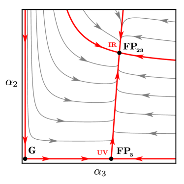
Figure 1: Template phase diagram for an MSSM-like quantum field theory with an interacting UV fixed point in the plane of the weak $(\alpha_{2})$ and strong $(\alpha_{3})$ gauge couplings, also showing an interacting IR fixed point, the free gaussian fixed point (G), and sample renormalisation group trajectories with arrows pointing towards the IR. Note that the gaussian must be a “saddle” with both relevant and irrelevant perturbations. Plot adopted from Bond:2017suy .

The outline of this paper is as follows. In Sec. II we review the renormalisation group equations for supersymmetric gauge theories with matter, and discuss necessary conditions and general features of perturbative fixed points. In Sec. III, we investigate UV and IR fixed points of the MSSM with conserved or broken $R$-parity. We further explain the rationale for several new types of MSSM extensions and determine their respective fixed points. In Sec. IV, we focus on the prospects of matching MSSM extensions with interacting UV fixed points to the SM at low energies. In Sec. V we discuss our results and conclude. Auxiliary information is provided in several appendices.

II Renormalisation Group for Supersymmetry

We consider $\mathcal{N}=1$ supersymmetric gauge theories with product gauge group

$$G=\prod_{a}G_{a}$$ (1)

and gauge couplings $g_{a}$, where the index $a$ runs over simple and abelian group factors. Throughout we scale loop factors into the definition of couplings and introduce

$$\alpha_{a}=g_{a}^{2}/(4\pi)^{2}\,.$$ (2)

We also consider chiral superfields $\Phi_{i}$, which may or may not carry local gauge charges, and which may further interact through a superpotential. Mass terms are of no relevance for this section and are neglected. Instead, we consider the most general superpotential with canonically marginal couplings but omit canonically irrelevant interactions, hence

$$W(\Phi)=\frac{1}{6}\,{Y}^{ijk}\,\Phi_{i}\,\Phi_{j}\,\Phi_{k}$$ (3)

with Yukawa couplings ${Y}^{ijk}$, ${Y}_{ijk}=({Y}^{ijk})^{*}$. Yukawa couplings are a necessity for asymptotically safe UV fixed points to occur at weak coupling Bond:2016dvk . We are particularly interested in theories which display interacting fixed points in the IR or UV. Conformal critical points correspond to free or interacting fixed points, which can be found using the renormalisation group equations.

A Renormalisation Group

In perturbation theory the renormalisation of the gauge couplings up to two-loop level in the $\overline{\text{DR}}$ scheme is given by Machacek:1983tz ; Martin:1993zk

$$\mu\frac{d\alpha_{a}}{d\mu}\equiv\beta_{a} = \alpha_{a}^{2}\left(-B_{a}\,+C_{ab}\,\alpha_{b}-2\,Y_{4,a}\right)\,,$$ (4)

with indices $a,b$ always referring to gauge couplings. The one-loop coefficients $B_{a}$ and the two-loop gauge coefficients $C_{ab}$ are given by

$$B_{a} =6\,C_{2}^{G_{a}}-2\,S^{R_{a}}_{2}\,,$$ (5)

$$C_{ab} =4\,C_{2}^{G_{a}}\left(S^{R_{a}}_{2}-3\,C_{2}^{G_{a}}\right)\delta_{ab}+8\,S^{R_{a}}_{2}\,C^{R_{b}}_{2}\,.$$ (6)

The subscripts $a,b$ on the quadratic Casimir $(C^{G}_{2})$ and on the Dynkin index ($S^{R}_{2}$) of the matter fields indicate the subgroup of $G$. Using (5) we may rewrite the two-loop term as

$$C_{ab}=8\,S^{R_{a}}_{2}\,C^{R_{b}}_{2}-2\,C_{2}^{G_{a}}\,B_{a}\,\delta_{ab}$$ (7)

in terms of the one-loop terms. Evidently, the mixing terms are manifestly non-negative ($C_{ab}\geq 0$ for $a\neq b$) for any semi-simple supersymmetric gauge theory. Also, for $B_{a}<0$ we have $C_{aa}>0$ (no sum) in any quantum field theory Bond:2016dvk .

The Yukawa couplings (3) contribute to the running of the gauge couplings (4) starting at the two-loop level, with

$$Y_{4,a} = Y_{ijk}\,Y^{ijk}\,{C}^{R_{a}}_{2}(k)/d(G_{a})\,,$$ (8)

and $d(G_{a})$ denotes the dimension of group $G_{a}$. Non-renormalisation theorems for the superpotential guarantee that the exact flow for the Yukawa couplings $\beta_{Y}=dY/d\ln\mu$ is given by

$$\mu\frac{d}{d\mu}Y^{ijk}=Y^{ij\ell}\,\gamma^{k}_{\ell}+(i\leftrightarrow k)+(j\leftrightarrow k)$$ (9)

to any order in perturbation theory. Here, $\gamma^{k}_{\ell}$ denote the anomalous dimension matrix of the chiral superfields. In perturbation theory, they read at one-loop

$$\begin{array}[]{rcl}\displaystyle\gamma{}^{(1)}{}^{k}_{\ell}&=&\displaystyle\frac{1}{2}Y_{ij\ell}\,Y^{ijk}-2\,\alpha_{a}\,C^{R_{a}}_{2}(k)\,\delta^{k}_{\ell}\,.\end{array}$$ (10)

B UV and IR Fixed Points

An important consistency condition arises through the flow of the superpotential couplings Martin:2000cr . Taking the sum of absolute values squared of all superpotential couplings, $|Y|^{2}=Y_{ijk}\,Y^{ijk}$, and also using (4), (10) we find

$$\frac{1}{12}\partial_{t}|Y|^{2} =d(R)|\gamma(R)|^{2}$$ (11)

$$+\alpha_{a}\,d(G_{a})\left(Y_{4,a}-4\,\alpha_{b}\,S^{R_{a}}_{2}\,C^{R_{b}}_{2}\right)\,,$$

with $t=\ln\mu$, $d(R)$ the dimension of the representation $R$, $\gamma(R)$ the chiral superfield anomalous dimension, and Yukawas rescaled as $Y_{ijk}\to Y_{ijk}/4\pi$. A fixed point requires the simultaneous vanishing of all beta functions. For the gauge couplings, $\beta_{a}=0$ implies

$$2Y_{4,a}^{*} =-B_{a}+C_{ab}\,\alpha_{b}^{*}\,,$$ (12)

see (4). Expressions with an ’$*$’ -superscript are understood as being evaluated at a fixed point. Using (7), (11), and (12), we then find from $\partial_{t}|Y|^{2}=0$ that

$$d(R)|\gamma_{*}(R)|^{2} =\mbox{\small{$\frac{1}{2}$}}\,B_{a}\,\alpha^{*}_{a}\,d(G_{a})\left(1+2\,C_{2}^{G_{a}}\,\alpha^{*}_{a}\right)$$ (13)

must hold true for any fixed point. Since the left-hand-side is by definition a positive number, positivity of the weighted sum

$$d(G_{a})\,B_{a}\,\alpha^{*}_{a}>0\quad\text{together with}\quad\alpha_{a}^{*}\geq 0$$ (14)

is a necessary condition for interacting fixed points Bond:2017suy . For theories with a single gauge group this implies that asymptotically non-free theories $(B_{a}<0)$ cannot develop interacting fixed points Martin:2000cr ; Bond:2017suy . However, for theories with several gauge groups, (14) mandates that at least one of the gauge factors is asymptotically free Bond:2017suy , illustrated in Fig. 1.

A useful simplification arises through choices in the Yukawa sector (see App.A for more details), in which case the set of Yukawa couplings $\{Y_{ij\ell}\}$ can be mapped onto a set $\{y_{i}\}$ such that the RG beta functions for the Yukawa couplings squared are proportional to themselves. We may then introduce the Yukawa couplings as

$$\alpha_{i}=y_{i}^{2}/(4\pi)^{2}\,,$$ (15)

and the beta functions (9) with (10) turn into

$$\mu\frac{\partial\alpha_{i}}{\partial\mu}\equiv\beta_{i}=\alpha_{i}\left[\sum_{j}E_{ij}\alpha_{j}-\sum_{a}F_{ia}\alpha_{a}\right]\;,$$ (16)

characterised by the one-loop matrix $E_{ij}$ from superpotential contributions and the one-loop matrix $F_{ia}$ of gauge field contributions. Throughout, indices $i,j$ relate to Yukawa couplings while indices $a,b$ relate to gauge couplings (to avoid confusion, we also have written out the required summations explicitly). Moreover, the two-loop Yukawa term (8) simplifies into a linear combination of the Yukawa couplings,

$$Y_{4,a}=\mbox{\small{$\frac{1}{2}$}}\sum_{i}D_{ai}\,\alpha_{i}$$ (17)

for some coefficients $D_{ai}>0$. In these conventions, the beta functions for the gauge couplings (4) reads

$$\beta_{a}=\alpha_{a}^{2}\left[-B_{a}+\sum_{b}C_{ab}\,\alpha_{b}-\sum_{i}D_{ai}\,\alpha_{i}\right]\;,$$ (18)

with the one-loop coefficients $B_{a}$, the two-loop matrix $C_{ab}$ of gauge field contributions and the two-loop matrix $D_{ai}$ from the superpotential. In general, the elements of the matrices $D,E$ and $F$ are positive or zero.

At weak coupling, theories may display Banks-Zaks (BZ) fixed points and/or gauge-Yukawa (GY) fixed points Bond:2016dvk . The former are always IR, while the latter can be IR or UV. BZ fixed points are the solutions to $\beta_{a}/\alpha_{a}^{2}=0$ with vanishing superpotential couplings $\alpha_{i}=0$, leading to

$$B_{a}=\sum_{b}C_{ab}\,\alpha_{b}^{*}$$ (19)

for each of the non-vanishing gauge couplings. Further, gauge-Yukawa fixed points additionally have non-vanishing superpotential couplings. In this case, assuming that the matrix $E$ can be inverted, we can solve $\beta_{i}/\alpha_{i}=0$ using (16) to find the nullcline relation

$$\alpha_{i}^{*}=\sum_{j,a}(E^{-1})_{ij}\,F_{ja}\,\alpha_{a}^{*}\,,$$ (20)

relating the non-vanishing Yukawa couplings to the gauge couplings. After inserting (20) into (18), and demanding that $\beta_{a}/\alpha_{a}^{2}=0$, we find the fixed point condition

$$B_{a}=\sum_{b}C^{\prime}_{ab}\,\alpha_{b}^{*}$$ (21)

for each of the non-vanishing gauge couplings. The matrix $C^{\prime}$ can be viewed as a Yukawa-shifted two-loop matrix,

$$C^{\prime}_{ab}=C_{ab}-\sum_{i,j}D_{ai}\,(E^{-1})_{ij}\,F_{jb}\;,$$ (22)

which follows from (7) and (18) after inserting (20). As such, the shift $C\to C^{\prime}$ takes into account the fact that the superpotential couplings achieve a simultaneous fixed point.

In the following it turns out to be convenient to introduce a notation to differentiate between different types of fixed points. If gauge couplings $\alpha_{a}$, $\alpha_{b},\cdots$ remain non-zero at a fixed point, we refer to it as ${\rm FP}_{ab\cdots}$, where the indices relate to the non-zero gauge couplings, see Tab. 1. Additionally, Yukawa couplings may or may not be non-zero.

C Two Gauge Sectors

To be concrete, we discuss a model with two gauge couplings $\alpha_{2}$ and $\alpha_{3}$ and a superpotential, and with (4). This serves as a template for the $SU(2)\times SU(3)$ sector of MSSM extensions which is the focus of the following sections. We are interested in interacting UV or IR fixed point in settings where asymptotic freedom is absent. Hence, (14) mandates

$$B_{3}>0>B_{2}\,,$$ (23)

or the other way around, but not both $B_{2,3}<0$. With (23), $\alpha_{2}$ is a marginally irrelevant coupling close to the Gaussian, but it may become (marginally) relevant close to an interacting fixed point $\alpha^{*}_{3}$. In this setting, the sole BZ fixed point (19) is given by

$$\alpha_{3}^{*}=\frac{B_{3}}{C_{33}}\,,\quad\alpha_{2}^{*}=0\,.$$ (24)

The option $\alpha_{2}^{*}>0$ is not available because $B_{2}<0$ with (7) entails $C_{22}>0$. In turn, two options arise for GY fixed points (21). First, the GY fixed point may be partially interacting $({\rm FP}_{3})$, in which case

$$\alpha_{3}^{*}=\frac{B_{3}}{C^{\prime}_{33}}\,,\quad\alpha_{2}^{*}=0$$ (25)

alongside a non-trivial superpotential coupling. It requires that the shifted two-loop coefficient $C^{\prime}_{33}$ is positive. For this partially interacting fixed point to become a UV fixed point, it is required that $\alpha_{2}$ becomes marginally relevant in its vicinity (see Fig. 1). Expanding $\beta_{2}$ for small $\alpha_{2}$ and in the vicinity of the interacting fixed point, we find

$$\beta_{2}\big{|}_{{\rm FP}_{3}}=B_{2,\rm eff}\,\alpha_{2}^{2}+{\cal O}(\alpha_{2}^{3})\,,$$ (26)

with the effective one-loop coefficient $B_{2,\rm eff}$ now given by

$$B_{2,\rm eff}=B_{2}-C^{\prime}_{23}\,\alpha_{3}^{*}\,.$$ (27)

Hence, the sufficient condition for the fixed point ${\rm FP}_{3}$ to be UV reads

$$B_{2,\rm eff}>0>B_{2}\,.$$ (28)

which requires $C^{\prime}_{23}<0$.

Second, the required fixed point may be fully interacting $({\rm FP}_{23})$. Using (21) one obtains

$$\alpha_{3}^{*} =\frac{B_{3}\,C^{\prime}_{22}-B_{2}\,C^{\prime}_{32}}{C^{\prime}_{33}\,C^{\prime}_{22}-C^{\prime}_{23}\,C^{\prime}_{32}}\,,$$ (29)

$$\alpha_{2}^{*} =\frac{B_{2}\,C^{\prime}_{33}-B_{3}\,C^{\prime}_{23}}{C^{\prime}_{33}\,C^{\prime}_{22}-C^{\prime}_{23}\,C^{\prime}_{32}}$$ (30)

to leading order in perturbation theory. Whether fixed points of this type are UV or IR depends on the eigenvalue spectrum of the stability matrix. Fig. 1 illustrates the scenario in which the partially interacting GY fixed point ${\rm FP}_{3}$ is UV, and the fully interacting ${\rm FP}_{23}$ is IR. Most notably, $\alpha_{2}$ has become marginally relevant owing to interactions at ${\rm FP}_{3}$.

Fixed Point	Gauge Couplings			Type
$\text{FP}_{0}$	$\alpha_{3}^{*}=0$	$\ \ \ \alpha_{2}^{*}=0\ \ \$	$\alpha_{1}^{*}=0$	free
$\text{FP}_{1}$	$\alpha_{3}^{*}=0$	$\alpha_{2}^{*}=0$	$\alpha_{1}^{*}>0$	interacting
$\text{FP}_{2}$	$\alpha_{3}^{*}=0$	$\alpha_{2}^{*}>0$	$\alpha_{1}^{*}=0$	interacting
$\text{FP}_{3}$	$\alpha_{3}^{*}>0$	$\alpha_{2}^{*}=0$	$\alpha_{1}^{*}=0$	interacting
$\text{FP}_{12}$	$\alpha_{3}^{*}=0$	$\alpha_{2}^{*}>0$	$\alpha_{1}^{*}>0$	interacting
$\text{FP}_{13}$	$\alpha_{3}^{*}>0$	$\alpha_{2}^{*}=0$	$\alpha_{1}^{*}>0$	interacting
$\text{FP}_{23}$	$\alpha_{3}^{*}>0$	$\alpha_{2}^{*}>0$	$\alpha_{1}^{*}=0$	interacting
$\text{FP}_{123}$	$\alpha_{3}^{*}>0$	$\alpha_{2}^{*}>0$	$\alpha_{1}^{*}>0$	interacting

Table 1: Classification of fixed points according to the values of gauge couplings. Fixed points may be UV provided one or more Yukawa couplings are non-vanishing at the fixed point.

III MSSM and Extensions

In this section we investigate fixed points of the MSSM with conserved (Sec. A) and broken $R$-parity (Sec. B). We then put forward strategies for interacting fixed points in MSSM extensions based on additional matter fields and Yukawa interactions (Sec. C), and analyse three characteristic types of extensions in full detail (Secs. D – F).

A MSSM with $R$-Parity

We consider the SM gauge group

$$G_{\text{SM}}=SU(3)_{C}\times SU(2)_{L}\times U(1)_{Y}$$ (31)

and denote the hypercharge, the weak and strong gauge couplings as $\alpha_{1},\alpha_{2},$ and $\alpha_{3}$, respectively, with $\alpha_{a}=g_{a}^{2}/(4\pi)^{2}$ $(a=1,2,3)$ and $g_{a}$ the gauge couplings. The (left-handed) chiral superfields of the MSSM are summarised in Tab. 2. Consequently, the MSSM one-loop and two-loop gauge beta coefficients in (18) are given by

$$\begin{array}[]{llll}B_{1}=-22\;,&C_{11}=\frac{398}{9}\;,&C_{12}=18\;,&C_{13}=\frac{176}{3}\;,\\ B_{2}=-2\;,&C_{21}=6\;,&C_{22}=50\;,&C_{23}=48\;,\\ B_{3}=6\;,&C_{31}=\frac{22}{3}\;,&C_{32}=18\;,&C_{33}=28\;.\end{array}$$ (35)

Notice that $B_{2}<0$ and $B_{1}<0$ imply that the hypercharge and the weak gauge sector are not asymptotically free, and imply that the running gauge couplings $\alpha_{1}$ and $\alpha_{2}$ may both terminate in UV Landau poles unless they run into a fixed point in the UV.

In principle, there may arise up to seven distinct classes of interacting fixed points depending on whether one, two, or three of the gauge couplings remain non-zero at the fixed point. For want of language, we distinguish these using the terminology of Tab. 1. For example, the class of fixed points FP₃ refers to all possible fixed points where the hypercharge and weak gauge couplings vanish, the strong gauge coupling remains non-zero, and none, some, or all of the Yukawa couplings are non-zero. Notice that for fixed points of any type to be UV, at least one of the Yukawa couplings must be non-zero.

Superfield	$\bm{SU(3)_{C}}$	$\bm{SU(2)_{L}}$	$\bm{U(1)_{Y}}$	Multiplicity
quark doublets $Q$	3	2	$+\frac{1}{6}$	$3$
up-quark singlets $\overline{u}$	$\overline{\textbf{3}}$	1	$-\frac{2}{3}$	$3$
down-quark singlets $\overline{d}$	$\overline{\textbf{3}}$	1	$+\frac{1}{3}$	$3$
lepton doublets $L$	1	2	$-\frac{1}{2}$	$3$
lepton singlets $\overline{e}$	1	1	$+1$	$3$
up-Higgs $H_{u}$	1	2	$+\frac{1}{2}$	$1$
down-Higgs $H_{d}$	1	2	$-\frac{1}{2}$	$1$

Table 2: Summary of left-handed superfields in the MSSM.

Next, we turn to the superpotential of the MSSM. Besides anomaly-cancellation, we also impose invariance under $R$-parity Farrar:1978xj ; Dreiner:1997uz , characterised by the global $\text{U}(1)$ symmetry

$$P_{R}=(-1)^{3(B-L)+2s}\,.$$ (36)

Here $B$ , $L$ and $s$ are baryon number, lepton number and spin, respectively. The $R$-parity conserving superpotential of the MSSM reads

$$\begin{aligned} W_{\text{MSSM}}=&\ Y_{d}^{ij}\overline{d}_{i}Q_{j}H_{d}+Y_{u}^{ij}\overline{u}_{i}Q_{j}H_{u}+Y_{e}^{ij}\overline{e}_{i}L_{j}H_{d}\\ &+\mu H_{u}H_{d}\;,\end{aligned}$$ (37)

where $i,j=1,2,3$ correspond to flavor degrees of freedom, while gauge indices have been suppressed. As such, the MSSM may have up to $N_{Y}=27$ in general complex-valued Yukawa couplings. In this work, we are mostly interested in the case where the Yukawa matrices $Y_{e}$, $Y_{d}$ and $Y_{u}$ in (37) are approximated by $Y_{e}\approx 0$, $Y_{d}\approx\text{diag}(0,0,y_{b})$, $Y_{u}\approx\text{diag}(0,0,y_{t})$ with $y_{b}$ and $y_{t}$ denoting the bottom and top Yukawa couplings, respectively. The $\mu$-term is a mass term and does not play any role in the high energy limit of the theory and can be ignored in our study. The MSSM superpotential therefore reads

$$W_{\text{MSSM}}\approx y_{b}\overline{d}_{3}Q_{3}H_{d}+y_{t}\overline{u}_{3}Q_{3}H_{u}\;.$$ (38)

It constitutes the backbone for the MSSM and MSSM extensions studied in the following.

We now turn to the fixed points of the MSSM with the $R$-parity conserving superpotential (38). In addition to the gauge beta functions we have the Yukawa beta functions for the bottom and top couplings $\alpha_{b,t}=|y_{b,t}|^{2}/(4\pi)^{2}$, thus a total of three gauge and two Yukawa couplings,

$$\{\alpha_{1},\alpha_{2},\alpha_{3},\alpha_{b},\alpha_{t}\}\;.$$ (39)

The beta functions (16) for the bottom and top Yukawas are given by

$$\begin{aligned} \beta_{b}&=\alpha_{b}\bigg{[}12\alpha_{b}+2\alpha_{t}-\frac{14}{9}\alpha_{1}-6\alpha_{2}-\frac{32}{3}\alpha_{3}\bigg{]}\;,\\ \beta_{t}&=\alpha_{t}\bigg{[}12\alpha_{t}+2\alpha_{b}-\frac{26}{9}\alpha_{1}-6\alpha_{2}-\frac{32}{3}\alpha_{3}\bigg{]}\;.\end{aligned}$$ (40)

The bottom and top Yukawa nullclines (20), defined as the relations of couplings along which the top and bottom Yukawa beta functions (40) vanish, are given by

$$\begin{aligned} &\alpha_{b}=\frac{29}{315}\alpha_{1}+\frac{3}{7}\alpha_{2}+\frac{16}{21}\alpha_{3}\,,\\ &\alpha_{t}=\frac{71}{315}\alpha_{1}+\frac{3}{7}\alpha_{2}+\frac{16}{21}\alpha_{3}\;.\end{aligned}$$ (41)

Inserting these into the gauge beta functions (18) with the MSSM coefficients (35), and also using the two-loop Yukawa corrections to the running of the gauge couplings in (18)

$$\begin{aligned} D_{1b}&=\frac{28}{3}\;,\;D_{1t}=\frac{52}{3}\;,\;\\ D_{2b}&=12\;,\;\;D_{2t}=12\;,\;\\ D_{3b}&=8\;,\;\;\;\;D_{3t}=8\ \;,\end{aligned}$$ (42)

we are able to identify fixed point candidates. Since the hypercharge and $SU(2)$ beta functions are both asymptotically non-free ($B_{1},B_{2}<0$), the only possibility for an interacting fixed point in perturbation theory requires $B_{3}\,\alpha_{3}^{*}>0$, see (14). We find that all interacting fixed point candidates of the type $\text{FP}_{13}$, $\text{FP}_{23}$, or $\text{FP}_{123}$ invariably imply either $\alpha_{1}^{*}<0$ or $\alpha_{2}^{*}<0$, which is unphysical. The only viable setting is a fixed point of the type $\text{FP}_{3}$, with trivial $(\alpha_{1},\alpha_{2})|_{*}=(0,0)$ and non-trivial coordinates

$$\begin{aligned} \left.(\alpha_{3},\alpha_{b},\alpha_{t})\right|_{*}&=(\mbox{\small{$\frac{63}{166}$}},\mbox{\small{$\frac{24}{83}$}},\mbox{\small{$\frac{24}{83}$}})\\ &\approx(0.38,0.29,0.29)\;.\end{aligned}$$ (43)

Notice that both Yukawa couplings come out non-zero and unified. The effective one-loop coefficients $B_{1,\text{eff}}$ and $B_{2,\text{eff}}$ (28) are negative

$$\begin{array}[]{rcl}B_{1,\text{eff}}&=&-\mbox{\small{$\frac{1102}{83}$}}\approx-13.3\;,\\ B_{2,\text{eff}}&=&-\mbox{\small{$\frac{4242}{83}$}}\approx-51.1\;,\end{array}$$ (44)

implying that the gauge-Yukawa fixed point of the MSSM is IR. We have also explicitly checked that this conclusion is robust against including the tau Yukawa coupling, and against further finite entries in $Y_{d}$, $Y_{u}$ and $Y_{e}$ of the MSSM superpotential (37).
 We conclude that the MSSM does not offer interacting UV fixed points to the leading orders in perturbation theory. For investigations of IR fixed points or quasi IR fixed points in the MSSM or MSSM GUTs, we refer to the studies in Allanach:1996nj ; Lanzagorta:1995ai ; Kobayashi:1996zu ; Codoban:1999fp ; Aulakh:2008sn ; Abel:1998yi ; Huang:2000rn ; Nevzorov:2013ixa ; Casas:1998vh ; Barger:1993vu ; Bardeen:1993rv .

B MSSM without $R$-Parity

We now turn to the $R$-parity violating (RPV) MSSM with superpotential

$$\begin{aligned} W_{\text{RPV}}&=W_{\text{MSSM}}+\lambda^{\prime ijk}\overline{d}_{i}Q_{j}L_{k}+\frac{1}{2}\lambda^{ijk}L_{i}L_{j}\overline{e}_{k}\\ &+\frac{1}{2}\lambda^{\prime\prime ijk}\overline{u}_{i}\overline{d}_{j}\overline{d}_{k}+\mu^{\prime i}L_{i}H_{u}\;.\end{aligned}$$ (45)

The first term in (45) is the MSSM superpotential provided earlier. The second and third terms change lepton number by one unit, $\Delta L=1$, and the fourth term changes baryon number by one unit, $\Delta B=1$. The $\mu^{\prime}$ term is a mass term irrelevant in the high energy limit. We therefore observe that the violation of $R$-parity results in lepton and baryon number violating processes, which may be relevant in processes like proton decay. Due to the non-observation of such processes, either the $\lambda$, $\lambda^{\prime}$, $\mu^{\prime}$ and $\lambda^{\prime\prime}$ couplings in (45) have to be small or superpartner masses are large Dawson:1985vr ; Barbieri:1985ty ; Barger:1989rk ; Godbole:1992fb ; Bhattacharyya:1995pq ; Dreiner:1997uz ; Domingo:2018qfg . The RPV MSSM may have up to $N_{Y}=108$ independent Yukawa couplings, four times as many as the $R$-parity preserving MSSM. Moreover, for each of the interacting fixed point classes of Tab. 1 may have up to $2^{N_{Y}}$ different fixed points, depending on which of the Yukawa couplings are vanishing or non-vanishing.

We now search for fixed points in the RPV MSSM. To avoid constraints due to proton decay, we concentrate on the $\lambda^{\prime}$ terms, with flavor indices $i,j,k=1,2,3$,

$$\lambda^{\prime ijk}\overline{d}_{i}Q_{j}L_{k}\;.$$ (46)

Hence, in addition to the top and bottom Yukawa couplings of the MSSM, we retain the RPV Yukawa couplings $\lambda^{\prime}_{ijk}$. For the sequel, we define

$$\alpha_{\lambda^{\prime}_{ijk}}=\frac{|\lambda^{\prime}_{ijk}|^{2}}{(4\pi)^{2}}\,.$$ (47)

To avoid models with non-linear nullcline conditions (see App.A) we limit ourselves here in the RPV MSSM and the MSSM extensions studied in Secs D – F to superpotentials with permutation flavor symmetries or with dangerous terms switched off by selection rules. Here, we introduce for each lepton species $k=1,2,3$ a universal matrix $(\lambda^{\prime k})_{ij}=\lambda^{\prime ijk}$, with

$$\mathbf{\lambda}^{\prime k}=\lambda^{\prime}\begin{pmatrix}\mathbf{M}&&0\\ 0&&0\\ \end{pmatrix}\,.$$ (48)

Here, $\mathbf{M}$ is a $2\times 2$ matrix with entries either one or zero. We denote by $I_{1}$ the number of times an entry ’1’ appears in $\mathbf{M}$, $1\leq I_{1}\leq 4$, excluding the MSSM-limit ($I_{1}=0$) and the symmetry-breaking case with $I_{1}=3$. The number of remaining different matrices is 11. To avoid non-linear Yukawa nullclines we do not allow for third generation quark couplings in $\lambda^{\prime k}$ as top and bottom already appear in $W_{\text{MSSM}}$. This leads to a set of $n=3I_{1}$ additional Yukawa couplings (47) which we denote as

$$\text{RPV Yukawa couplings: }\{\alpha_{4},\cdots,\alpha_{n+4}\}\;,$$

thus leading to a total of $3$ gauge and $2+n$ Yukawa couplings. In our analysis ($I_{1}\leq 4$), we have retained up to $n\leq 12$ RPV Yukawa couplings. The evolution of the Yukawa couplings are controlled by (40) together with

$$\begin{aligned} \beta_{\lambda^{\prime}}&=\alpha_{\lambda^{\prime}}\bigg{[}36I_{1}\alpha_{\lambda^{\prime}}-\frac{14}{9}\alpha_{1}-6\alpha_{2}-\frac{32}{3}\alpha_{3}\bigg{]}\;.\end{aligned}$$ (49)

Here, due to the symmetries of (48), the one-loop beta functions for $\alpha_{\lambda^{\prime}_{ijk}}\rightarrow\alpha_{\lambda^{\prime}}$ are identical, although their values do not need to be identical due to possibly different initial conditions.

Fixed points can be found from inserting the nullcline of (49) into the gauge beta functions (18) with the MSSM coefficients (35), and also noting that the two-loop Yukawa contributions to the running of the gauge couplings take the form

$$\begin{aligned} &D_{1b}=\frac{28}{3}\;,\;&D_{1t}&=\frac{52}{3}\;,\;&D_{1\lambda^{\prime}}&=28I_{1}\;,\\ &D_{2b}=12\;,\;&D_{2t}&=12\;,\;&D_{2\lambda^{\prime}}&=36I_{1}\;,\\[2.15277pt] &D_{3b}=8\;,\;&D_{3t}&=8\;,\;&D_{3\lambda^{\prime}}&=24I_{1}\;.\end{aligned}$$ (50)

We find that the only viable interacting fixed point is of the FP₃ type, with trivial $(\alpha_{1},\alpha_{2})|_{*}=(0,0)$ and

$$\begin{aligned} (\alpha_{3},\alpha_{b},\alpha_{t},\alpha_{\lambda^{\prime}})|_{*}&=(\mbox{\small{$\frac{189}{274}$}},\mbox{\small{$\frac{72}{137}$}},\mbox{\small{$\frac{72}{137}$}},\mbox{\small{$\frac{28}{137I_{1}}$}})\\ &\approx(0.69,0.53,0.53,\mbox{\small{$\frac{0.20}{I_{1}}$}})\;.\end{aligned}$$ (51)

Notice that $\alpha_{\lambda^{\prime}}^{*}$ now stands for any of the different RPV Yukawas, all of which take the same finite fixed point value. The fixed point is IR attractive and some of its couplings are large. We observe that the RPV MSSM is not offering interacting UV fixed points.

Superfield	$\bm{SU(3)_{C}}$	$\bm{SU(2)_{L}}$	$\bm{U(1)_{Y}}$	MSSM	Extension I	Extension II	Extension III
quark doublet $Q$	3	2	$+\mbox{\small{$\frac{1}{6}$}}$	$3$	$3$	$4$	$4$
anti-quark doublet $\overline{Q}$	$\overline{\textbf{3}}$	$\overline{\textbf{2}}$	$-\mbox{\small{$\frac{1}{6}$}}$	$0$	0	$1$	0
up-quark $\overline{u}$	$\overline{\textbf{3}}$	1	$-\mbox{\small{$\frac{2}{3}$}}$	$3$	$3+n_{u}$	$3$	$4$
down-quark $\overline{d}$	$\overline{\textbf{3}}$	1	$+\frac{1}{3}$	$3$	$3+n_{d}$	$3$	$4$
anti-up-quark $u$	3	1	$+\mbox{\small{$\frac{2}{3}$}}$	$0$	$n_{u}$	$0$	$0$
anti-down-quark $d$	3	1	$-\mbox{\small{$\frac{1}{3}$}}$	$0$	$n_{d}$	$0$	$0$
lepton doublet $L$	1	2	$-\mbox{\small{$\frac{1}{2}$}}$	$3$	$3+n_{L}$	$3+n_{L}$	$4+n_{L}$
anti-lepton doublet $\overline{L}$	1	$\overline{\textbf{2}}$	$+\mbox{\small{$\frac{1}{2}$}}$	$0$	$n_{L}$	$n_{L}$	$n_{L}$
lepton singlet $\overline{e}$	1	1	$+1$	$3$	3	3	$4$
up-Higgs $H_{u}$	1	2	$+\mbox{\small{$\frac{1}{2}$}}$	$1$	1	1	$1$
down-Higgs $H_{d}$	1	2	$-\mbox{\small{$\frac{1}{2}$}}$	1	1	$1$	$1$
gauge singlets $S$	1	1	0	$0$	$0$	$n_{S}$	$0$

Table 3: Field content of different types of MSSM extensions in comparison with the MSSM, also showing gauge charges of superfields under the SM gauge groups.

C Constructing MSSM Extensions

Next, we turn to extensions of the MSSM and the prospect for interacting UV or IR fixed points. One may hope to find an interacting UV fixed point provided that the Gaussian corresponds to a saddle point Bond:2017suy . Hence, at least one gauge sector should remain asymptotically free while another one should be infrared free. In our setting, the hypercharge one-loop gauge coefficient $(B_{1})$ is always negative, and remains negative in any extension. Further, for the MSSM, we are in the scenario where the non-Abelian gauge factors obey (23). Hence, the one-loop gauge coefficient of the weak coupling $(B_{2})$ is negative, and will remain negative in any extension. On the other hand, the one-loop coefficient of the strong coupling in the MSSM reads $B_{3}=6$, thus leaving room for a finite number of additional colored superfields.

Specifically, each additional superfield in the representation $R$ of $SU(3)_{C}$ lowers $B_{3}$ by $2S_{3}(R)$. For the fundamental or anti-fundamental representation holds $S_{3}=\frac{1}{2}$, of which one needs one each to avoid gauge anomalies. The sextet and anti-sextet representations have $S_{3}=\frac{5}{2}$, yet gauge anomaly cancellation dictates to include at least two of these, yielding a wrong-sign $B_{3}$ of $-4$. The representation with the next higher Dynkin index is the adjoint, which is real with $S_{3}=3$, however, a single one of them leads already to $B_{3}=0$. All other, higher representations have $S_{3}>3$ and are therefore not viable. We conclude that there are only two possibilities to add colored BSM superfields which keep $B_{3}$ positive, either one pair, or two pairs of (fundamental, anti-fundamental) $SU(3)_{C}$ chiral superfields. These arguments do not limit the number of colorless fields, such as leptons.

We are therefore led to three types of MSSM extensions:

• New quark singlets and new leptons. On top of the MSSM fields, type I models display $n_{u}$ additional pairs of up-quark singlets $(u,\overline{u})$, $n_{d}$ new down-quark singlets $(d,\overline{d})$, and $n_{L}$ additional lepton doublet pairs ($L$, $\overline{L}$).

• New quark doublets and new leptons. These models display two additional quark doublets ($Q_{4},\overline{Q}_{1}$), $n_{L}$ additional lepton and anti-lepton doublet pairs ($L$, $\overline{L}$).

• A fourth generation and new leptons. These extensions display a fourth generation with new superfields ($Q_{4}$, $\overline{u}_{4}$, $\overline{d}_{4}$, $L_{4}$), and $n_{L}$ new lepton and anti-lepton doublet pairs ($L$, $\overline{L}$).

In addition, we also have the liberty to add $n_{S}$ gauge singlet fields $S_{i}$ and suitable Yukawa couplings involving MSSM and BSM matter fields. We find that the impact of singlets for fixed points is subleading except in type II models, which is why we include them there and only there. The field content of the MSSM extensions is summarised in Tab. 3, also showing the SM gauge charges of matter fields. Note that we are not concerned with the $U(1)_{Y}$ sector, which remains infrared free. This is viable phenomenologically as long as the $U(1)_{Y}$ Landau pole arises beyond the Planck scale. Extensions which also aim at stabilising $U(1)_{Y}$ will be considered elsewhere. In the following, we investigate the availability of interacting fixed points for each of these settings in detail.

D New Quark Singlets and Leptons

We begin with the first type of MSSM extension by adding BSM quark singlets as well as lepton doublets to the MSSM. The BSM particle content (see Tab 3) is characterised, respectively, by the number of beyond-MSSM $(u,\bar{u})$, $(d,\bar{d})$ and $(L,\bar{L})$ pairs,

$$n_{u}\;,\;n_{d}\;,\;n_{L}\;,$$ (52)

Asymptotic freedom of the strong force is lost for $n_{u}+n_{d}\geq 3$. A priori, no upper limits apply on $n_{L}$. The number of matter fields beyond the MSSM is

$$N_{\text{BSM}}=N_{q,\text{BSM}}+N_{L,\text{BSM}}\,.$$ (53)

where $N_{q,\text{BSM}}=2(n_{u}+n_{d})$ and $N_{L,\text{BSM}}=2n_{L}$ are the new quark singlets and lepton doublets, respectively, and where we count fermions and anti-fermions separately. The most general gauge invariant and perturbatively renormalisable superpotential then reads

$$\begin{aligned} W_{1}=&\ Y^{ijk}\overline{d}_{i}Q_{j}L_{k}+\overline{Y}^{ijk}\overline{u}_{i}Q_{j}\overline{L}_{k}\\ &+x_{b}\,y_{b}\overline{d}_{3}Q_{3}H_{d}+x_{t}\,y_{t}\overline{u}_{3}Q_{3}H_{u}\;,\end{aligned}$$ (54)

with top and bottom Yukawas denoted by $y_{t}$ and $y_{b}$, and BSM Yukawas $Y^{ijk}$ and $\overline{Y}^{ijk}$. Here $i,j,k$ denote flavor indices, while gauge indices are suppressed. The parameters $x_{b,t}\in\{0,1\}$ allow us to switch the bottom and top Yukawas on and off. In terms of the BSM matter field multiplicities (52), the superpotential (54) has up to

$$N_{Y}^{\text{general}}=3(3+n_{d})(n_{L}+3)+3(3+n_{u})n_{L}+2$$ (55)

independent Yukawa couplings. In the fixed point search, we focus on a subset of all possible non-zero Yukawa couplings, parameterized by the following set of integers

$$x_{b}\,,\;x_{t}\,,\;I_{12}\,,\;I_{13}\,,\;I_{1d}\,,\;I_{2d}\,,\;I_{3d}\,,\;I_{1u}\,,\;I_{2u}\,,\;I_{3u}\,.$$ (56)

These integers, if positive, indicate which type of Yukawa couplings in (54) are taken to be non-zero, and how many of them are retained. Specifically, we are interested in superpotentials (54) which retain

$$\begin{aligned} \text{\text@underline{type of monomial}}&:\text{\text@underline{how many of them}}\\ y_{b}\,\overline{d}_{3}\,Q_{3}\,H_{d}&:x_{b}\;,\\ y_{t}\,\overline{u}_{3}\,Q_{3}\,H_{u}&:x_{t}\;,\\ y_{4}\,\overline{d}_{i}\,Q_{1}\,L_{k}+y_{6}\,\overline{d}_{i}\,Q_{2}\,L_{k^{\prime}}&:I_{12}\;,\\ y_{5}\,\overline{d}_{i}\,Q_{1}\,L_{k}&:I_{1d}\;,\\ y_{7}\,\overline{d}_{i}\,Q_{2}\,L_{k}&:I_{2d}\;,\\ y_{8}\,\overline{d}_{i}\,Q_{1}\,L_{k}+y_{9}\,\overline{d}_{i}\,Q_{3}\,L_{k^{\prime}}&:I_{13}\;,\\ y_{10}\,\overline{d}_{i}\,Q_{3}\,L_{k}&:I_{3d}\;,\\ y_{11}\,\overline{u}_{i}\,Q_{1}\overline{L}_{k}&:I_{1u}\;,\\ y_{12}\,\overline{u}_{i}\,Q_{2}\overline{L}_{k}&:I_{2u}\;,\\ y_{13}\,\overline{u}_{i}\,Q_{3}\overline{L}_{k}&:I_{3u}\;.\end{aligned}$$ (57)

We again label couplings as indicated in footnote ${}^{\ref{foot:4})}$. To avoid non-linear nullclines we also made choices as in the analysis of the RPV MSSM (Sec. B). Let us explain the construction principle leading to (57):

• The bottom and top quarks $\overline{d}_{3}$ and $\overline{u}_{3}$ are only allowed in the bottom or top Yukawa terms already present in the MSSM, see (38). They can be switched on and off individually with the parameters $x_{b},x_{t}\in\{1,0\}$.

• Superfields $\overline{d}_{i}$, $i\neq 3$ that is, any of them but not the third generation may appear in exactly one superpotential term. This can still be more than one term, one for each $i\neq 3$. The number of times any $\overline{d}_{i}$, $i\neq 3$, appears exactly once together with $Q_{1}$, $Q_{2}$, or $Q_{3}$ is given by $I_{1d}$, $I_{2d}$, and $I_{3d}$, respectively.

• The same as $(ii)$ but for up-type singlets: The number of times any $\overline{u}_{i}$, $i\neq 3$, appears exactly once together with $Q_{1}$, $Q_{2}$, or $Q_{3}$ is given by $I_{1u}$, $I_{2u}$, and $I_{3u}$, respectively.

• Down-type quarks $\overline{d}_{i}$, $i\neq 3$ may be present in two different Yukawa monomials. With $I_{12}$ ($I_{13})$ we count down quark superfields $\overline{d}_{i},i\neq 3$ appearing exactly twice, once with $Q_{1}$ and once with $Q_{2}$ ($Q_{3}$).

• Each lepton doublet $L$ and anti-lepton doublet $\overline{L}$ (both MSSM and BSM) is allowed at most once in the superpotential.

A concrete benchmark model where this machinery can be seen at work is given in Sec. A.

The reduced set of Yukawa interactions (57) is the result of an extensive trial and error search. In fact, we have initially performed scans within the much wider set of superpotentials (54), but noticed that viable fixed point candidates do not arise without down-quarks $\bar{d}_{i}$, $i\neq 3$ appearing twice in the superpotential. Moreover, we also noticed that ultraviolet fixed points cannot be found if we allow for lepton doublets to appear twice in the superpotential with each quark singlet appearing at most once. We believe that our selection of Yukawa structures are the simplest ones to enable viable fixed points.

As a result, in terms of (56) the number of independent Yukawa couplings retained in our investigations reads

$$N_{Y}=2(I_{12}+I_{13})+\sum\limits_{i=1}^{3}(I_{id}+I_{iu})+x_{b}+x_{t}\;.$$ (58)

This is only a small subset of the formally allowed superpotential terms (55), yet, suffices to identify interacting gauge-Yukawa fixed points.

By construction, the models are described by three gauge and $N_{Y}$ independent Yukawa couplings. Due to remaining flavor symmetries acting on quark singlets and on lepton doublets appearing in terms of the same Yukawa coupling type, we encounter at most 12 different types of Yukawa beta functions corresponding to those of the bottom and top Yukawas, and the 10 couplings $y_{i}$ introduced in (57), modulo copies thereof, see Sec. A for an example where symmetries reduce the number of independent beta functions. The beta functions for the Yukawa couplings are given in App.C.

Next, we detail the results of the fixed point search. The selection rules i) - v) still allow for infinitely many MSSM extensions. However, the number of new quark singlets is bounded from above ($N_{q,{\rm BSM}}=2(n_{u}+n_{d})\leq 4$, see Sec. C) or else weakly-interacting fixed points cannot arise in perturbation theory. Similarly, increasing the number of new leptons makes the weak gauge coupling more infrared-free, and it becomes increasingly challenging if not outright impossible to find ultraviolet fixed points. For these reasons, we limit new matter field multiplicities as follows

$$\begin{aligned} &0\leq n_{d}\leq 2-n_{u}\;,\\ &0\leq n_{u}\leq 2-n_{d}\;,\\ &0\leq n_{L}\leq 11\,.\end{aligned}$$ (59)

The set of Yukawa couplings is restricted by

$$\begin{aligned} &0\leq I_{1u}\leq I_{2u}\,,\\ &0\leq x_{b}\,,x_{t}\leq 1\,,\\ &0\leq I_{12}\,,\,I_{13}\,,\,I_{1d}\,,\,I_{2d}\,,\,I_{3d}\,,\,I_{1u}\,,\,I_{2u}\,,\,I_{3u}\leq 4\,.\end{aligned}$$ (60)

Overall, the above choices cover 112.600 different MSSM extensions with up to $N_{Y}=12$ independent Yukawa couplings. Amongst these, we find 109.926 settings with viable IR fixed points. Further, 114 models also show candidates for interacting UV fixed points. Also, a small set of models do not show interacting fixed point despite the strong gauge sector remaining asymptotically free. The reason for this is that the Yukawa-induced corrections are so strong that the fixed point becomes unphysical in pertubation theory $(\alpha_{3}<0)$. These settings would require a non-perturbative check.

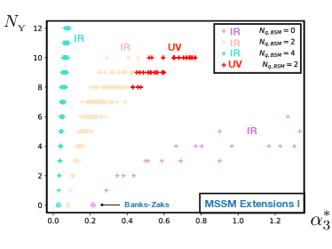
Figure 2: Fixed points of MSSM extensions (type I). Shown are the fixed point values $\alpha_{3}^{*}$ against the number of Yukawa couplings $N_{Y}$, corresponding to 109.926 models, see text. The color coding indicates the number of additional quark singlets $N_{q,\text{BSM}}=2(n_{u}+n_{d})$, and whether the fixed point is UV or IR. 114 models have an UV $\text{FP}_{3}$ (in red).

More specifically, in all models considered we find that fixed points, if they arise, remain interacting in the strong gauge sector with

$$0.027\approx\frac{3}{110}\lesssim\alpha_{3}^{*}\big{|}_{\text{FP}_{3}}\,,$$ (61)

in agreement with the analytical expression (109). The weak and hypercharge gauge interactions are either switched off (in which case fixed points are of the type $\text{FP}_{3}$), or the weak coupling remains non-zero as well (when fixed points are of the type $\text{FP}_{23}$), see Tab. 1. Fixed points with vanishing strong gauge coupling, that is, $\text{FP}_{1}$, $\text{FP}_{2}$, or $\text{FP}_{12}$, or fixed points with all gauge couplings non-zero ($\text{FP}_{123}$) do not arise (see App.B).

As an aside, we have verified explicitly that no interacting fixed points arise once $N_{q,{\rm BSM}}\geq 6$ by scanning 3.434.836 models including up to 4 pairs of singlet quarks, confirming the reasoning put forward in Sec. C.

All fixed points with both non-abelian gauge couplings interacting, i.e. $\alpha_{3}^{*}>0$ and $\alpha_{2}^{*}>0$, and trivial or non-trivial superpotential couplings turn out to be infrared. In turn, the fixed points of the type $\text{FP}_{3}$ are found to be either infrared or ultraviolet. If they are infrared, all gauge and non-trivial superpotential couplings are irrelevant. Most importantly, there are no outgoing RG trajectories along which the weak gauge coupling can be switched on. Moreover, none of the models with infrared $\text{FP}_{3}$ have a simultaneous fixed point of the type $\text{FP}_{23}$.

In Fig. 2, we show the strong gauge coupling for all fixed points of the type $\text{FP}_{3}$. Also displayed are the number of non-trivial Yukawa couplings $N_{Y}$. Different numbers of new quark singlets $N_{q,\text{BSM}}$ lead to different branches of fixed points. Their color-coding relates to $N_{q,\text{BSM}}$ and whether the fixed point is infrared (magenta: $N_{q,{\rm BSM}}=0$, yellow: $N_{q,{\rm BSM}}=2$, green: $N_{q,{\rm BSM}}=4$) or ultraviolet (red: $N_{q,{\rm BSM}}=2$).

For $N_{Y}=0$, and for any $0\leq N_{q,\text{BSM}}\leq 4$ we find an infrared Banks-Zaks fixed point. For $N_{Y}>0$, fixed points are of the gauge-Yukawa type and can be IR or UV. For fixed $N_{Y}$, we observe that the strong coupling becomes larger with increasing $N_{q,{\rm BSM}}$. For fixed $N_{q,\text{BSM}}$, we also observe that the strong gauge coupling tends to increase with increasing $N_{Y}$.

For each strand of models, Fig. 2 indicates that the Banks-Zaks fixed point provides a lower bound on the strong coupling. The reason for this is that non-trivial Yukawa couplings reduce the effective two-loop coefficient and enhance $\alpha_{3}^{*}$. To the leading orders in perturbation theory, the lower bounds are $\alpha_{3}^{*}\geq\mbox{\small{$\frac{3}{14}$}}\approx 0.214$ for $N_{q,\rm BSM}=0$, $\alpha_{3}^{*}\geq\mbox{\small{$\frac{3}{38}$}}\approx 0.089$ for $N_{q,\rm BSM}=2$, and $\alpha_{3}^{*}\geq\mbox{\small{$\frac{3}{110}$}}\approx 0.027$ as at the minimum (61) for $N_{q,\rm BSM}=4$. Moreover, the models with $N_{q,\text{BSM}}=4$ (green points) lead to weakly interacting IR fixed points, and the threshold towards UV fixed points is not crossed. For models with $N_{q,\text{BSM}}=0$ (magenta points), the fixed point is more strongly interacting, and once more a regime with UV fixed points is not reached. Inbetween, the models with $N_{q,\text{BSM}}=2$ lead to weakly interacting IR fixed points for any $N_{Y}\leq 7$, and for some $N_{Y}>7$ (yellow points). Overall fixed points are mostly perturbative ($\alpha_{3}^{*}\ll 1$) though with increasing $N_{Y}$ some of the fixed points become borderline perturbative $(\alpha_{3}^{*}<1)$ or even strongly coupled $(\alpha_{3}^{*}\approx 1)$ such as in the $N_{q,\text{BSM}}=0$ strand.

Finally, provided that $N_{q,\text{BSM}}=2$, that is, either a pair of additional up-singlets $(u,\bar{u})$, or a pair of down-type ones $(d,\bar{d})$, and $N_{Y}=8,9$ or $10$, we also find models where the fixed point is UV with $\alpha_{2}$ becoming marginally relevant due to quantum effects (red points).

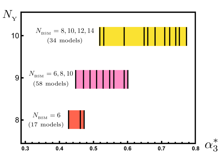
Figure 3: Spectroscopy of ultraviolet fixed points in type I models. Shown are the ranges of $\alpha_{3}^{*}$, sorted according to numbers of BSM Yukawa couplings $(N_{{}_{\rm Y}})$, and the number of BSM superfields $(N_{{}_{\rm BSM}})$ .

In Fig. 3 we show $\alpha_{3}^{*}$ at the UV fixed point as a function of the number of BSM Yukawa couplings $(N_{{}_{\rm Y}})$, and the number of BSM superfields $(N_{{}_{\rm BSM}})$. Evidently, the fixed point tends to become more strongly interacting the more independent Yukawa couplings are present. The settings with UV fixed points are further discussed in Sec. IV.

E New Quark Doublets and Leptons

For the second type of MSSM extensions, we introduce a quark doublet $Q_{4}$ and an anti-quark doublet $\overline{Q}_{1}$ as the new colored field content beyond the MSSM. Furthermore, we allow for $n_{L}$ pairs of BSM lepton and anti-lepton doublets $L$ and $\overline{L}$. We also include $n_{S}$ gauge singlet superfields $S$. The resulting superfield content (type II models) is summarized in Tab. 3. We study the superpotential

$$\begin{aligned} W_{2}&=Y^{ijk}\overline{d}_{i}Q_{j}L_{k}+\overline{Y}^{ijk}\overline{u}_{i}Q_{j}\overline{L}_{k}+Y^{i}_{S}S_{i}\overline{Q}_{1}Q_{4}\\ &+x_{b}y_{b}\overline{d}_{3}Q_{3}H_{d}+x_{t}y_{t}\overline{u}_{3}Q_{3}H_{u}\;,\end{aligned}$$ (62)

with $i,j,k$ summing over all flavor indices and $x_{b},x_{t}\in\{0,1\}$ are parameters which switch on and off the bottom and top Yukawa couplings. The first few terms of (62) resemble the non-MSSM terms of the superpotential (54) of model type I, with the difference that here $i$ and $j$ run over different numbers of flavors. We compensate for the smaller amount of quark singlets, present in the Yukawa terms of $Y^{ijk}$ and $\overline{Y}^{ijk}$, by including terms with Yukawa couplings $Y_{S}^{i}$ involving the new anti-quark doublet $\overline{Q}_{1}$. The number of generally possible non-zero Yukawa couplings in the superpotential (62) is

$$\begin{aligned} N_{Y}^{\text{general}}&=3\cdot 4\cdot(n_{L}+3)+3\cdot 4\cdot n_{L}+n_{S}+2\\ &=24n_{L}+38+n_{S}\;,\end{aligned}$$ (63)

with each term of the first line counts the number of Yukawa couplings in the respective term of the superpotential (62).

To parametrize different models efficiently, we introduce $n_{L}$ and $n_{S}$ to count leptons and singlets. Further, the non-zero Yukawa couplings in (62) are parametrised by the integers

$$I_{Q},\;I_{d}\;,\;I_{u}\;,\;x_{3}\;,\;\overline{x}_{3}\;,\;x_{4}\;,\;\overline{x}_{4}\;,\;x_{S}\;,\;x_{b}\;,\;x_{t}\;,$$ (64)

which count the different types of monomials appearing in the superpotential according to

$$\begin{aligned} \text{\text@underline{type of monomial}}&:\text{\text@underline{how many of them}}\\ y_{b}\,\overline{d}_{3}\,Q_{3}\,H_{d}&:x_{b}\;,\\ y_{t}\,\overline{u}_{3}\,Q_{3}\,H_{u}&:x_{t}\;,\\ y_{4}\,\overline{d}_{1,2}\,Q_{1,2}\,L_{k}&:I_{d}\cdot I_{Q}\;,\\ y_{5}\,\overline{u}_{1,2}\,Q_{1,2}\,\overline{L}_{k}&:I_{u}\cdot I_{Q}\;,\\ y_{6}\,\overline{d}_{3}\,Q_{1,2}\,L_{k}&:x_{3}\cdot I_{Q}\;,\\ y_{7}\,\overline{u}_{3}\,Q_{1,2}\,\overline{L}_{k}&:\overline{x}_{3}\cdot I_{Q}\;,\\ y_{8}\,\overline{d}_{1,2}\,Q_{4}\,L_{k}&:x_{4}\cdot I_{d}\;,\\ y_{9}\,\overline{u}_{1,2}\,Q_{4}\,\overline{L}_{k}&:\overline{x}_{4}\cdot I_{u}\;,\\ y_{10}\,S_{i}\,\overline{Q}_{1}\,Q_{4}&:x_{\text{S}}\cdot n_{\text{S}}\;.\end{aligned}$$ (65)

The selection of superpotentials with (64), (65) from general superpotentials (62) is similar in spirit to the choices we made previously for the MSSM with quark singlet extensions (type I). Further details including all RG beta functions are detailed in App.D.

To illustrate the construction principle, we consider a subset of terms from (62)

$$\begin{aligned} W_{2}\supset&\ Y^{111}\overline{d}_{1}Q_{1}L_{1}+Y^{142}\overline{d}_{1}Q_{4}L_{2}+\overline{Y}^{111}\overline{u}_{1}Q_{1}\overline{L}_{1}\\ &+Y^{313}\overline{d}_{3}Q_{1}L_{3}+\overline{Y}^{312}\overline{u}_{3}Q_{1}\overline{L}_{2}\\ &+Y_{S}^{1}S_{1}\overline{Q}_{1}Q_{4}+y_{b}\overline{d}_{3}Q_{3}H_{d}+y_{t}\overline{u}_{3}Q_{3}H_{u}\;.\end{aligned}$$ (66)

It corresponds to the parameters

$$\begin{aligned} &x_{3}=\overline{x}_{3}=x_{4}=x_{S}=x_{b}=x_{t}=1,\\ &\overline{x}_{4}=0\;,\ I_{d}=I_{u}=I_{Q}=n_{S}=1\;,\end{aligned}$$

with $n_{L}\geq 2$. The map from (66) to (65) is given by

$$\begin{aligned} &Y^{111}\leftrightarrow y_{4}\;,\;Y^{142}\leftrightarrow y_{8}\;,\;Y^{313}\leftrightarrow y_{6}\;,\;\\ &\overline{Y}^{111}\leftrightarrow y_{5}\;,\;\overline{Y}^{312}\leftrightarrow y_{7}\;,\;Y_{S}^{1}\leftrightarrow y_{10}\end{aligned}$$

and the expressions for the Yukawa and gauge beta functions (16), (18) can be found in App.D.

Within the general model setup (65) we scanned 79.920 models in the parameter ranges

$$\begin{aligned} &1\leq n_{S}\leq 5\;,\qquad\;\;0\leq n_{L}\leq 8\;,\\ &0\leq I_{d}\;,\;I_{u}\leq 2\;,\quad 1\leq I_{Q}\leq 2\;,\quad\\ &0\leq x_{3}\;,\;\overline{x}_{3}\;,\;x_{4}\;,\;\overline{x}_{4}\;,\;x_{S}\;,\;x_{b}\;,\;x_{t}\leq 1\;.\end{aligned}$$ (67)

We find that amongst all possible interacting fixed points (see Tab. 1) only those of the type $\text{FP}_{3}$ where $\alpha_{3}^{*}\neq 0$ are realised. $\text{FP}_{3}$ can be either of the Banks-Zaks type or of the gauge-Yukawa type (25). It exists for all models and is found to be IR and perturbative, with the strong gauge coupling fixed point in the range

$$0.027\lesssim\alpha_{3}^{*}\big{|}_{\text{FP}_{3}}\lesssim 0.08\;.$$ (68)

The numerical lower bound is in agreement with the bound dictated by the leading order in perturbation theory, (61). We do not find instances where the fixed point $\text{FP}_{3}$ becomes ultraviolet.

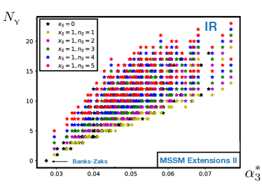
Figure 4: Fixed points of MSSM extensions (type II). Shown are the values for the strong coupling constant $\alpha_{3}^{*}$ at the $\text{FP}_{3}$ fixed point for all 79.920 MSSM extensions of type II given by the chiral superfields of Tab. 3 and superpotential (62). Fixed points are IR throughout. Also shown is the number of Yukawa couplings $N_{Y}$ (69). Fixed points become slightly more strongly interacting with increasing number of Yukawa couplings.

In Fig. 4, we compare the value of $\alpha_{3}$ at $\text{FP}_{3}$ against the number of Yukawa couplings $N_{Y}$ for all scanned models. We observe that gauge-Yukawa fixed points are more strongly interacting than the Banks-Zaks fixed point. Moreover, all fixed points are infrared and do not qualify as UV completions for the theory. Notice that our setup retains up to

$$\begin{aligned} N_{Y}&=(I_{d}+x_{3}+I_{u}+\overline{x}_{3})I_{Q}\\ &+x_{4}I_{d}+\overline{x}_{4}I_{u}+x_{S}n_{S}+x_{b}+x_{t}\;,\end{aligned}$$ (69)

different Yukawa couplings. Of these, the scan (67) covered models with up to $N_{Y}=23$. From Fig. 4, we learn that models tend to become more strongly interacting the more Yukawa couplings are switched on. Hence, although our scan only covered a small fraction of the $N_{Y,\text{scan}}^{\text{general}}=307$ different Yukawa couplings that could have been retained according to (63), (67), we do not expect that they would have opened a window for weakly coupled UV fixed points.

F Fourth Generation and New Leptons

Here, we turn to MSSM extensions involving fourth generation quark doublet $Q_{4}$, and quark singlets $\overline{d}_{4}$ and $\overline{u}_{4}$. To avoid gauge anomalies, a fourth lepton generation consisting of a lepton doublet $L_{4}$ and a lepton singlet $\overline{e}_{4}$ are added as well. In addition, we allow for $n_{L}$ pairs of leptons and anti-leptons $(L,\overline{L})$ (see Tab. 3). The superpotential reads

$$\begin{aligned} W_{3}=&\ Y^{ijk}\overline{d}_{i}Q_{j}L_{k}+\overline{Y}^{ijk}\overline{u}_{i}Q_{j}\overline{L}_{k}\\ &+y_{b}\overline{d}_{3}Q_{3}H_{d}+y_{t}\overline{u}_{3}Q_{3}H_{u}\;,\end{aligned}$$ (70)

which looks similar to (54) of type I models. The main difference is the presence of $Q_{4}$ in (70), and that non-trivial bottom- and top Yukawa interactions are considered from the outset. Note, possible terms $\bar{u}_{4}Q_{4}H_{u}$ and $\bar{d}_{4}Q_{4}H_{d}$ have not been included to avoid multiple appearances of the fourth generation, and corresponding challenges, see App.A. The maximal number of non-zero Yukawa couplings in $W_{3}$ is given by

$$\begin{aligned} N_{Y}^{\text{general}}&=4\cdot 4\cdot(n_{L}+4)+4\cdot 4\cdot n_{L}+2\\ &=32n_{L}+66\;.\end{aligned}$$ (71)

Our models are characterised by the number $n_{L}$ of BSM lepton pairs, and integers

$$I_{1d},\;I_{3d},\;I_{12},\;I_{13},\;I_{14},\;I_{1u},\;I_{4u}\;$$ (72)

characterising the Yukawa interactions in (70) as

$$\begin{aligned} \text{\text@underline{type of monomial}}&:\text{\text@underline{how many of them}}\\ y_{b}\overline{d}_{3}Q_{3}H_{d}&:1\,,\\ y_{t}\overline{u}_{3}Q_{3}H_{u}&:1\,,\\ y_{4}\overline{d}_{i}Q_{1}L_{k}+y_{5}\overline{d}_{i}Q_{2}L_{k^{\prime}}&:I_{12}\;,\\ y_{6}\overline{d}_{i}Q_{1}L_{k}+y_{7}\overline{d}_{i}Q_{3}L_{k^{\prime}}&:I_{13}\;,\\ y_{8}\overline{d}_{i}Q_{1}L_{k}+y_{9}\overline{d}_{i}Q_{4}L_{k^{\prime}}&:I_{14}\;,\\ y_{10}\overline{d}_{i}Q_{1}L_{k}&:I_{1d}\;,\\ y_{11}\overline{d}_{i}Q_{3}L_{k}&:I_{3d}\;,\\ y_{12}\overline{u}_{i}Q_{1}\overline{L}_{k}&:I_{1u}\;,\\ y_{13}\overline{u}_{i}Q_{4}\overline{L}_{k}&:I_{4u}\;.\end{aligned}$$ (73)

Flavor symmetries limit the number of different BSM beta functions in (73) to be at most 10 ($\beta_{4},...,\beta_{13}$). All beta functions, and further details are given in App.E.

Based on this ansatz, we have scanned 3.868 models within the ranges

$$\begin{aligned} &0\leq I_{12},I_{13},I_{14},I_{1d},I_{3d},I_{1u},I_{4u}\leq 3\;,\\ &0\leq n_{L}\leq 8\;.\end{aligned}$$ (74)

Once more, we find that only $\text{FP}_{3}$ arises, with any of the other fixed point candidates coming out as unphysical. Moreover, whenever it arises, $\text{FP}_{3}$ is numerically small with couplings in the range

$$0.027\lesssim\alpha_{3}^{*}|_{\text{FP}_{3}}\lesssim 0.10\;,$$ (75)

and in accord with the lower bound on the gauge coupling fixed point found to the leading orders in perturbation theory, (61). In total, we find that all 3.868 different models show conformal fixed points of the type $\text{FP}_{3}$, all of which are infrared. We neither find any other types of fixed points, nor candidates for ultraviolet fixed points.

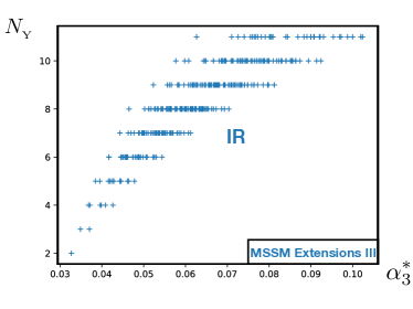
Figure 5: Fixed points of MSSM extensions (type III). Shown is $\alpha_{3}^{*}$ at the fixed point $\text{FP}_{3}$ for models with superpotential (70), corresponding to the 3.868 different models. All fixed points are IR and perturbative. Also shown is the number of Yukawa couplings $N_{Y}$ (76). The fixed point tends to become more strongly interacting with larger $N_{Y}$.

No.	$n_{u}$	$n_{d}$	$n_{L}$	$I_{12}$	$I_{13}$	$I_{1d}$	$I_{2d}$	$I_{3d}$	$I_{1u}$	$I_{2u}$	$I_{3u}$	$\bm{N}_{{}_{\rm\bf BSM}}$	$\bm{N}_{{}_{\rm\bf Y}}$	$\bm{\alpha_{{}_{3}}^{*}}$
1	0	1	2	0	1	1	1	0	0	1	1	6	8	0.431
2	0	1	2	1	0	0	2	0	1	1	0	6	8	0.431
3	0	1	2	1	0	1	1	0	0	2	0	6	8	0.431
4	0	1	2	0	1	0	1	1	1	1	0	6	8	0.431
5	0	1	2	0	1	1	0	1	0	2	0	6	8	0.431
6	0	1	2	1	0	2	0	0	1	1	0	6	8	0.431
7	0	1	2	0	1	0	2	0	1	1	0	6	8	0.458
8	0	1	2	0	1	1	1	0	0	2	0	6	8	0.458
9	0	1	2	1	0	0	1	1	1	1	0	6	8	0.458
10	0	1	2	1	0	1	0	1	0	2	0	6	8	0.458
11	0	1	2	1	0	1	0	1	1	1	0	6	8	0.458
12	0	1	2	1	0	1	1	0	0	1	1	6	8	0.458
13	0	1	2	1	0	2	0	0	0	1	1	6	8	0.458
14	0	1	2	0	1	1	1	0	1	1	0	6	8	0.473
15	0	1	2	1	0	1	1	0	1	1	0	6	8	0.473
16	0	1	2	1	0	2	0	0	0	2	0	6	8	0.473
17	0	1	2	0	1	2	0	0	0	2	0	6	8	0.473
18	0	1	2	0	2	1	0	0	1	1	0	6	9	0.452
19	0	1	2	2	0	0	1	0	0	2	0	6	9	0.468
20	0	1	2	0	2	0	0	1	0	2	0	6	9	0.468
21	0	1	2	0	2	0	1	0	0	1	1	6	9	0.468
22	0	1	2	2	0	0	1	0	0	0	2	6	9	0.488
23	0	1	2	2	0	1	0	0	0	0	2	6	9	0.488
24	0	1	2	2	0	0	0	1	0	1	1	6	9	0.488
25	0	1	2	1	1	0	0	1	0	2	0	6	9	0.514
26	0	1	2	1	1	0	1	0	0	1	1	6	9	0.514
27	0	1	2	1	1	0	1	0	0	2	0	6	9	0.514
28	1	0	3	1	1	0	0	0	0	2	1	8	9	0.514
29	1	0	3	1	1	0	0	0	0	3	0	8	9	0.514
30	0	1	3	1	1	0	0	1	0	2	0	8	9	0.514
31	0	1	3	1	1	0	1	0	0	1	1	8	9	0.514
32	0	1	3	1	1	0	1	0	0	2	0	8	9	0.514
33	0	1	2	0	2	0	1	0	0	2	0	6	9	0.526
34	0	1	2	2	0	0	0	1	0	2	0	6	9	0.526
35	0	1	2	2	0	0	1	0	0	1	1	6	9	0.526
36	1	0	3	0	2	0	0	0	0	3	0	8	9	0.526
37	0	1	3	0	2	0	1	0	0	2	0	8	9	0.526
38	1	0	3	2	0	0	0	0	0	2	1	8	9	0.526
39	0	1	3	2	0	0	0	1	0	2	0	8	9	0.526
40	0	1	3	2	0	0	1	0	0	1	1	8	9	0.526
41	0	1	2	1	1	0	0	1	1	1	0	6	9	0.528
42	0	1	2	1	1	1	0	0	0	1	1	6	9	0.528
43	1	0	3	1	1	0	0	0	1	1	1	8	9	0.528
44	0	1	3	1	1	0	0	1	1	1	0	8	9	0.528
45	0	1	3	1	1	1	0	0	0	1	1	8	9	0.528
46	0	1	2	1	1	1	0	0	1	1	0	6	9	0.547
47	0	1	3	1	1	1	0	0	1	1	0	8	9	0.547
48	0	1	2	2	0	1	0	0	1	1	0	6	9	0.561
49	0	1	3	2	0	1	0	0	1	1	0	8	9	0.561
50	0	1	2	0	2	0	1	0	1	1	0	6	9	0.561
51	0	1	2	0	2	1	0	0	0	2	0	6	9	0.561
52	0	1	2	2	0	0	1	0	1	1	0	6	9	0.561
53	0	1	2	2	0	1	0	0	0	2	0	6	9	0.561
54	1	0	3	0	2	0	0	0	1	2	0	8	9	0.561
55	0	1	3	0	2	0	1	0	1	1	0	8	9	0.561
56	0	1	3	0	2	1	0	0	0	2	0	8	9	0.561
57	1	0	3	2	0	0	0	0	1	2	0	8	9	0.561

No.	$n_{u}$	$n_{d}$	$n_{L}$	$I_{12}$	$I_{13}$	$I_{1d}$	$I_{2d}$	$I_{3d}$	$I_{1u}$	$I_{2u}$	$I_{3u}$	$\bm{N}_{{}_{\rm\bf BSM}}$	$\bm{N}_{{}_{\rm\bf Y}}$	$\bm{\alpha_{{}_{3}}^{*}}$
58	0	1	3	2	0	0	1	0	1	1	0	8	9	0.561
59	0	1	3	2	0	1	0	0	0	2	0	8	9	0.561
60	0	1	2	2	0	0	0	1	1	1	0	6	9	0.591
61	0	1	2	2	0	1	0	0	0	1	1	6	9	0.591
62	0	1	3	2	0	1	0	0	0	1	1	8	9	0.591
63	0	1	3	2	0	0	0	1	1	1	0	8	9	0.591
64	1	0	3	2	0	0	0	0	1	1	1	8	9	0.591
65	1	0	4	2	0	0	0	0	1	1	1	10	9	0.591
66	0	1	4	2	0	0	0	1	1	1	0	10	9	0.591
67	0	1	4	2	0	1	0	0	0	1	1	10	9	0.591
68	0	1	2	1	1	0	1	0	1	1	0	6	9	0.598
69	0	1	2	1	1	1	0	0	0	2	0	6	9	0.598
70	1	0	3	1	1	0	0	0	1	2	0	8	9	0.598
71	0	1	3	1	1	0	1	0	1	1	0	8	9	0.598
72	0	1	3	1	1	1	0	0	0	2	0	8	9	0.598
73	1	0	4	1	1	0	0	0	1	2	0	10	9	0.598
74	0	1	4	1	1	0	1	0	1	1	0	10	9	0.598
75	0	1	4	1	1	1	0	0	0	2	0	10	9	0.598
76	0	1	3	0	3	0	0	0	1	1	0	8	10	0.519
77	0	1	3	2	1	0	0	0	0	0	2	8	10	0.533
78	0	1	3	1	2	0	0	0	0	1	1	8	10	0.594
79	0	1	4	1	2	0	0	0	0	1	1	10	10	0.594
80	0	1	3	0	3	0	0	0	0	2	0	8	10	0.652
81	0	1	3	3	0	0	0	0	0	2	0	8	10	0.652
82	0	1	4	0	3	0	0	0	0	2	0	10	10	0.652
83	0	1	4	3	0	0	0	0	0	2	0	10	10	0.652
84	0	1	5	0	3	0	0	0	0	2	0	12	10	0.652
85	0	1	5	3	0	0	0	0	0	2	0	12	10	0.652
86	0	1	3	3	0	0	0	0	0	0	2	8	10	0.655
87	0	1	4	3	0	0	0	0	0	0	2	10	10	0.655
88	0	1	5	3	0	0	0	0	0	0	2	12	10	0.655
89	0	1	3	1	2	0	0	0	1	1	0	8	10	0.680
90	0	1	4	1	2	0	0	0	1	1	0	10	10	0.680
91	0	1	5	1	2	0	0	0	1	1	0	12	10	0.680
92	0	1	3	2	1	0	0	0	0	1	1	8	10	0.705
93	0	1	4	2	1	0	0	0	0	1	1	10	10	0.705
94	0	1	5	2	1	0	0	0	0	1	1	12	10	0.705
95	0	1	3	3	0	0	0	0	1	1	0	8	10	0.722
96	0	1	4	3	0	0	0	0	1	1	0	10	10	0.722
97	0	1	5	3	0	0	0	0	1	1	0	12	10	0.722
98	0	1	6	3	0	0	0	0	1	1	0	14	10	0.722
99	0	1	3	2	1	0	0	0	0	2	0	8	10	0.738
100	0	1	4	2	1	0	0	0	0	2	0	10	10	0.738
101	0	1	5	2	1	0	0	0	0	2	0	12	10	0.738
102	0	1	6	2	1	0	0	0	0	2	0	14	10	0.738
103	0	1	3	1	2	0	0	0	0	2	0	8	10	0.738
104	0	1	4	1	2	0	0	0	0	2	0	10	10	0.738
105	0	1	5	1	2	0	0	0	0	2	0	12	10	0.738
106	0	1	6	1	2	0	0	0	0	2	0	14	10	0.738
107	0	1	3	3	0	0	0	0	0	1	1	8	10	0.750
108	0	1	4	3	0	0	0	0	0	1	1	10	10	0.750
109	0	1	5	3	0	0	0	0	0	1	1	12	10	0.750
110	0	1	6	3	0	0	0	0	0	1	1	14	10	0.750
111	0	1	3	2	1	0	0	0	1	1	0	8	10	0.767
112	0	1	4	2	1	0	0	0	1	1	0	10	10	0.767
113	0	1	5	2	1	0	0	0	1	1	0	12	10	0.767
114	0	1	6	2	1	0	0	0	1	1	0	14	10	0.767

Table 4: Overview of the UV fixed points candidates in type I models obtained in Sec. D. Shown is the number of left-handed up-type quark singlets $(n_{u})$, down-type quark singlets $(n_{d})$, and lepton $(n_{L})$ chiral superfields, the parameters (56) characterising the superpotential, the total number of superfields ${N}_{{}_{\rm\bf BSM}}$ beyond the MSSM, the total number of non-trivial Yukawa couplings ${N}_{{}_{\rm\bf Y}}$, and the fixed point values ${\alpha_{{}_{3}}^{*}}$ (see main text). Models are ordered according to increasing ${N}_{{}_{\rm\bf Y}}$, ${\alpha_{{}_{3}}^{*}}$, and ${N}_{{}_{\rm\bf BSM}}$. A benchmark, model 7, discussed further in Sec. A is highlighted in blue.

In Fig. 5, we show $\alpha_{3}^{*}$ at $\text{FP}_{3}$ for all scanned type III models versus the number of Yukawa couplings $N_{Y}$. Again, we observe that $\alpha_{3}^{*}$ tends to grow for a larger numbers of Yukawa couplings. In our scans, the number of Yukawa couplings equals

$$N_{Y}=2\sum\limits_{i=2}^{4}I_{1i}+I_{1d}+I_{3d}+I_{1u}+I_{4u}+2\;.$$ (76)

Hence the scanned parameter space (74) covers models with up to $11$ interacting Yukawa couplings. Based on the structure of results, and also in comparison with the previous two models, we do not expect to find UV fixed points by increasing the number of independent Yukawas.

IV Ultraviolet Completions

In this section, we focus on MSSM extensions with ultraviolet fixed points and the prospects for matching them to the Standard Model at low energies.

A Main Features and Benchmark

In Sec. D, we obtained MSSM extensions with ultraviolet fixed points (type I models). They are summarised in Tab. 4 showing for each model the number of left-handed up-type quark singlets $(n_{u})$, down-type quark singlets $(n_{d})$, and lepton $(n_{L})$ chiral superfields, the parameters (56) characterising the superpotential (57), the total number of superfields ${N}_{{}_{\rm\bf BSM}}$ beyond the MSSM, the total number of non-trivial Yukawa couplings ${N}_{{}_{\rm\bf Y}}$, and the fixed point value of the strong coupling ${\alpha_{{}_{3}}^{*}}$. The models are sorted according to increasing ${N}_{{}_{\rm\bf Y}}$, ${\alpha_{{}_{3}}^{*}}$, and ${N}_{{}_{\rm\bf BSM}}$, in this order. For all models, we observe that the superpotential parameters obey $I_{12}+I_{13}+I_{1d}+I_{2d}+I_{3d}+I_{1u}+I_{2u}+I_{3u}=5$, and $I_{12}+I_{13}$ is either 1, 2 or 3. Furthermore, we always find that the MSSM bottom and top Yukawa couplings are interacting in the UV, and that $n_{u}+n_{d}=1$.

Models with UV fixed points and vanishing $\alpha_{2}^{*}$ always come with an associated IR fixed point where $\alpha_{2}^{*}$ remains non-zero. In Fig. 6, we compare the corresponding values of the strong gauge coupling. They are in the range

$$0.43\lesssim\alpha_{3}^{*}\big{|}_{\text{UV}}<\alpha_{3}^{*}\big{|}_{\text{IR}}\,.$$ (77)

Note that fixed points are borderline perturbative. As such, they must be taken with a grain of salt as higher loop corrections Novikov:1983uc ; Novikov:1985rd or non-perturbative effects Intriligator:2003jj ; HLM22 may well be of a similar magnitude. In Fig. 6, the black horizontal line indicates the onset of strong coupling $(\alpha_{3}\geq 1)$, which is the case for a few IR fixed points.

Our results are in accord with more formal constraints such as the $a$-theorem, which states that the central charge $a=\frac{3}{32}\left[2d_{G}+\sum_{i}(1-R_{i})(1-3(1-R_{i})^{2})\right]$must be a decreasing function along RG trajectories in any $4d$ quantum field theory Anselmi:1997am . Here, $d_{G}$ denotes the dimension of the gauge groups, $i$ runs over all chiral superfields, and $\gamma_{i}$ and $R_{i}=\mbox{\small{$\frac{2}{3}$}}(1+\gamma_{i})$ the corresponding anomalous dimensions and $R$-charges, respectively. We find

$$\Delta a=a_{\text{UV}}-a_{\text{IR}}>0$$ (78)

on any of the UV-IR connecting trajectories. Had the IR limit been the Gaussian, validity of the $a$-theorem would imply strong coupling and non-perturbatively large $R$-charges in the UV, at least for some of the fields. In our models, this cannot arise because the Gaussian is a saddle and the IR is not free. Hence, no trajectories connect the UV to the Gaussian, which supports the weak form of the $a$-theorem as $a_{\text{UV}}-a_{\text{G}}<0$. We have also checked that fixed points are in accord with the positivity of central charges, the conformal collider bound, and constraints from unitarity Cardy:1988cwa ; Osborn:1989td ; Anselmi:1997am ; Hofman:2008ar ; Komargodski:2011vj .

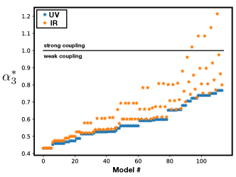
Figure 6: The strong gauge coupling $\alpha_{3}^{*}$ at the UV fixed point ($\text{FP}_{3}$) (blue stars) and the associated IR fixed point ($\text{FP}_{23}$) (orange stars) for type I models in Tab. 4. Models have two quark singlets beyond the MSSM, plus leptons.

Next, we focus on a benchmark, model 7 from Tab. 4 with blue background color, and matter content summarised in Tab. 5, and with the superpotential

$$\begin{aligned} W_{1}\supset&\,Y^{411}\overline{d}_{4}Q_{1}L_{1}+Y^{432}\overline{d}_{4}Q_{3}L_{2}+Y^{124}\overline{d}_{1}Q_{2}L_{4}\\ &+Y^{225}\overline{d}_{2}Q_{2}L_{5}+\overline{Y}^{211}\overline{u}_{2}Q_{1}\overline{L}_{1}\\ &+\overline{Y}^{122}\overline{u}_{1}Q_{2}\overline{L}_{2}+y_{b}\overline{d}_{3}Q_{3}H_{d}+y_{t}\overline{u}_{3}Q_{3}H_{u}\;.\end{aligned}$$ (79)

The model features the parameters

$$\begin{aligned} &I_{12}=I_{1d}=I_{3d}=I_{3u}=0\;,\\ &I_{13}=I_{1u}=I_{2u}=x_{b}=x_{t}=1\;,\\ &I_{2d}=2\;,n_{u}=0\;,\ n_{d}=1\;,\ n_{L}=2\;,\end{aligned}$$ (80)

see (57). Every term of the superpotential (79) contains exactly one superfield beyond the MSSM. Hence even though $R$-parity violation is a crucial feature of the superpotential (54), we can stay within experimental bounds in our benchmark model if the masses of these fields beyond the MSSM are large enough Dawson:1985vr ; Barbieri:1985ty ; Barger:1989rk ; Godbole:1992fb ; Bhattacharyya:1995pq ; Dreiner:1997uz ; Domingo:2018qfg . Further, the Yukawa couplings of (57) and (79) are related as

$$\begin{aligned} Y^{411}\rightarrow y_{8},\;\ Y^{432}\rightarrow y_{9},\;\ Y^{124}\rightarrow y_{7},\;\\ \overline{Y}^{211}\rightarrow y_{11},\;\overline{Y}^{122}\rightarrow y_{12},\;Y^{225}\rightarrow y_{7}\,,\end{aligned}$$ (81)

and $y_{4},y_{5},y_{6},y_{10},y_{13}=0$. Notice that the permutation flavor symmetry

$$(\overline{d}_{1},L_{4})\leftrightarrow(\overline{d}_{2},L_{5})\;.$$ (82)

implies that the RG beta functions for the couplings $Y^{124}$ and $Y^{225}$ are equivalent, and mapped onto the same type of beta function. The benchmark data is given in Tab. 6. All non-zero components of $\text{FP}_{23}$ are slightly larger than the corresponding couplings at $\text{FP}_{3}$.

Superfield	$\bm{SU(3)_{C}}$	$\bm{SU(2)_{L}}$	$\bm{U(1)_{Y}}$	Multiplicity
MSSM:   quark doublet $Q$	3	2	$+\mbox{\small{$\frac{1}{6}$}}$	$3$
up-quark singlet $\overline{u}$	$\overline{\textbf{3}}$	1	$-\mbox{\small{$\frac{2}{3}$}}$	$3$
down-quark singlet $\overline{d}$	$\overline{\textbf{3}}$	1	$+\mbox{\small{$\frac{1}{3}$}}$	$3$
lepton doublet $L$	1	2	$-\mbox{\small{$\frac{1}{2}$}}$	$3$
lepton singlet $\overline{e}$	1	1	$+1$	$3$
up-Higgs $H_{u}$	1	2	$+\mbox{\small{$\frac{1}{2}$}}$	$1$
down-Higgs $H_{d}$	1	2	$-\mbox{\small{$\frac{1}{2}$}}$	$1$
BSM:   quark singlet $\overline{d}_{4}$	$\overline{\textbf{3}}$	1	$+\mbox{\small{$\frac{1}{3}$}}$	$1$
anti-quark singlet $d_{1}$	3	1	$-\mbox{\small{$\frac{1}{3}$}}$	$1$
lepton doublets $L_{4,5}$	1	2	$-\mbox{\small{$\frac{1}{2}$}}$	$2$
anti-lepton doublets $\overline{L}_{1,2}$	1	$\overline{\textbf{2}}$	$+\mbox{\small{$\frac{1}{2}$}}$	$2$

Table 5: Summary of left-handed superfields in the benchmark model, also showing their gauge charges and multiplicity (model 7 of Tab. 4). The four bottom rows show the superfield content beyond the MSSM.

	$\bm{\alpha_{3}}$	$\bm{\alpha_{2}}$	$\bm{\alpha_{Y^{411}}}$	$\bm{\alpha_{Y^{432}}}$	$\bm{\alpha_{Y^{124}}}$	$\bm{\alpha_{Y^{225}}}$	$\bm{\alpha_{\overline{Y}^{211}}}$	$\bm{\alpha_{\overline{Y}^{122}}}$	$\bm{\alpha_{y_{t}}}$	$\bm{\alpha_{y_{b}}}$
$\bm{\text{\bf FP}_{3}}$	0.458	0	0.278	0.208	0.306	0.306	0.361	0.306	0.320	0.320
$\bm{\text{\bf FP}_{23}}$	0.474	0.025	0.296	0.222	0.326	0.326	0.385	0.326	0.341	0.341

Table 6: Coordinates of the UV and IR fixed points of the benchmark model (model 7 of Tab. 4).

Finally, we compare the benchmark superpotential (79) with a sample superpotential (66) which arises in models with additional quark doublets (see Sec. E). Neglecting hypercharge (so that $\overline{d}$ and $\overline{u}$ have the same gauge representations), we see that these two superpotentials differ in two aspects. Firstly, in (66), $\overline{u}_{3}$ appears once outside of $W_{\text{MSSM}}$, inducing a mixing with $y_{t}$ ($E_{t7}{\neq}0$ in App. D). Secondly, the term involving $\overline{Q}_{1}$ in (66) has its gauge indices contracted in a different manner than $Q_{2}$ in the superpotential (79), yielding a Yukawa self-coupling term of $E_{10,10}=16$ (see App. D) instead of $E_{12,12}=12$ (see App. C). While these differences are small in that they lead to only small differences in the beta functions, they suffice to alter the nature of the fixed point from UV to IR.

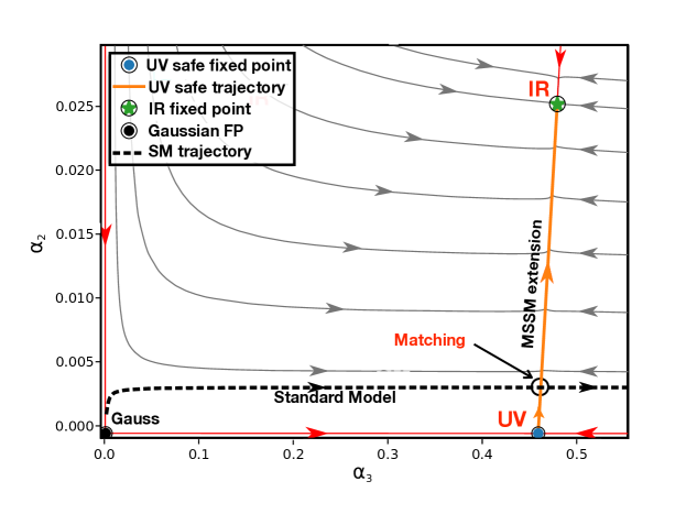
Figure 7: Shown are the RG flows of the benchmark model with particle content as in Tab. 5 and superpotential (79), projected onto the $(\alpha_{2},\alpha_{3})$ plane, and all Yukawas on their nullclines. Full dots show the Gaussian, the UV ($\text{FP}_{3}$), and the IR fixed point ($\text{FP}_{23}$), and arrows on trajectories point from the UV to the IR. We also indicate the SM running of gauge couplings (dashed black line), and the trajectory emanating from the UV fixed point (orange).

B Asymptotic Safety with Logarithmic Scaling and UV Critical Surface

In four dimensions, the free Gaussian fixed point of a gauge coupling corresponds to a double-zero of its beta function (4). This implies that the scaling dimension $\sim\partial_{\alpha}\beta(\alpha)|_{\alpha^{*}=0}$ vanishes, meaning that the running of asymptotically free gauge couplings becomes logarithmically slow close to the Gaussian. Conversely, interacting fixed points generically correspond to single zeros with $\partial_{\alpha}\beta(\alpha)|_{\alpha^{*}\neq 0}\neq 0$, which implies that the running of couplings becomes power law, and much faster.

Perhaps unexpectedly, however, it turns out that the RG scaling out of an interacting fixed point may still only be logarithmic in some cases. The reason for this is that fixed points may be partially interacting in gauge theories with product gauge groups, meaning that some of the gauge couplings are switched off at the fixed point. If so, the gauge couplings which vanish at the fixed point only run logarithmically, even if the other couplings achieve an interacting fixed point, $e.g.$ (26).

Here, this scenario is realised for all UV fixed points. Specifically, the weak gauge coupling vanishes in the UV, where it represents a marginally relevant interaction as in (26) with (27) and (28). In consequence, its RG running out of the fixed point is given by

$$\alpha_{2}(\mu)=\frac{\delta\alpha_{2}(\Lambda)}{1+B_{2,\rm eff}\,\delta\alpha_{2}\,\ln(\mu/\Lambda)}\,,$$ (83)

with $\delta\alpha_{2}(\Lambda)$ the sole free parameter of the theory at the high scale $\Lambda$, and $B_{2,\rm eff}>0$ the interaction-induced one-loop coefficient. Hence, despite of the theory being asymptotically safe with residual interactions in the UV, we find that the marginally relevant coupling $\alpha_{2}$ runs logarithmically as in asymptotic freedom. Further, dimensional transmutation leads to a RG invariant mass scale

$$\mu_{\rm tr}=\Lambda\exp\big{[}-{B_{2,\rm eff}\,\delta\alpha_{2}(\Lambda)}\big{]}^{-1}\,,$$ (84)

which is the analogue of the scale $\Lambda_{\rm QCD}$ in QCD, and independent of the high scale $\Lambda\gg\mu_{\rm tr}$ where the RG flow is started.

As an aside, we note that a power-law running of relevant perturbations out of a UV fixed point with supersymmetry can only arise if one or several of the asymptotically nonfree gauge couplings remain interacting in the UV. Here, this minimally requires an interacting fixed point of the type FP₂₃ with both $\alpha_{2}^{*}$ and $\alpha_{3}^{*}$ non-zero, and outgoing trajectories. Although this scenario does not arise in the models studied here (nor in the models of Bond:2017suy ) it would be useful to establish conditions under which power-law scaling becomes available.

Another feature of the fixed points is that the strong gauge coupling $\alpha_{3}$ and the non-trivial Yukawa couplings have become marginally irrelevant interactions in the UV. Their running is fully determined by the one of $\alpha_{2}$ along the outgoing trajectory, $\alpha_{3}(\mu)=F_{3}(\alpha_{2}(\mu))$ for the strong gauge coupling and $\alpha_{i}(\mu)=G_{i}(\alpha_{2}(\mu))$ for the non-trivial Yukawas, with $F_{3}(x)$ and $G_{i}(x)$ model-dependent functions. Close to the fixed point, this becomes

$$\alpha_{3}(\mu)=\alpha_{3}^{*}+A_{3}\,\alpha_{2}(\mu)$$ (85)

$$\alpha_{i}(\mu)=\alpha_{i}^{*}+B_{i}\,\alpha_{2}(\mu)$$

with $A_{3}$ and $B_{i}$ model-dependent parameters. Hence, all gauge and Yukawa couplings run logarithmically rather than power-law close to the partially interacting UV fixed point, which also percolates to other parameters including soft supersymmetry breaking terms or gaugino masses Martin:2000cr . Most notably, the UV critical surface has only one free parameter Bond:2017suy . This should be contrasted with asymptotic freedom where, instead, non-abelian gauge and Yukawa couplings are all marginally relevant. Hence, interacting UV fixed points with supersymmetry enhance the predictive power over asymptotically free models and over fixed point theories without supersymmetry Bond:2017suy .

C Matching to the Standard Model

We now discuss the phase diagram of the benchmark model, shown in Fig. 7, which is of the same form as anticipated in Fig. 1. Relevant perturbations such as $\delta\alpha_{2}$ can trigger outgoing RG flows. Specifically, Fig. 7 shows RG trajectories in the $(\alpha_{3},\alpha_{2})$ plane with Yukawas projected onto their nullcline values, and the various fixed points, which are the Gaussian, the UV ($\text{FP}_{3}$), and the IR fixed point ($\text{FP}_{23}$). Arrows on trajectories point from the UV to the IR, and coloured trajectories indicate separatrices between the various fixed points. The dashed black line indicates the SM running of gauge couplings, covering the range from MeV to Planckian energies. The UV safe trajectory emanating from the UV fixed point is depicted in orange. It would cross over into the IR fixed point provided all fields remain massless. Further, we note a bound for the IR fixed point value of the weak gauge coupling,

$$0.003<\alpha_{2}^{*}\big{|}_{\rm IR}\,,$$ (86)

or else the UV-IR connecting separatrix terminates at the IR fixed point before the SM line is ever reached. Then, to match the theory to the standard model, some fields need to decouple and become massive. If this happens at the appropriate energy scale, the UV safe trajectory can be matched to the SM, as indicated in Fig. 7.

Next, we determine the matching scale $\mu=\mu_{\rm SM}$. Recall that since the UV safe theory only has a single free parameter (83), $\alpha_{3}(\mu)$ is uniquely determined by $\alpha_{2}(\mu)$. Hence, the UV-safe trajectory relates the gauge couplings as $\alpha^{\rm UV}_{3}(\mu)\equiv\alpha_{3}(\alpha_{2}(\mu))$. Similarly, for the Standard Model we may express the RG running of the strong gauge coupling in terms of the weak gauge coupling and write $\alpha_{3}^{\rm SM}(\mu)\equiv\alpha_{3}^{\rm SM}(\alpha_{2}^{\rm SM}(\mu))$. The matching scale is then uniquely determined from the condition $\alpha_{3}^{\rm UV}=\alpha_{3}^{\rm SM}$, which has a unique solution for $\alpha_{2}(\mu_{\rm SM})$ (see Fig. 7). We find

$$\mu_{\rm SM}\lesssim\mathcal{O}($1\text{\,}\mathrm{GeV}\text{/}$)$$ (87)

for the benchmark model of Tab. 5, and, for that matter, for any of the models in Tab. 4. Hence, despite of the remarkable fact that the MSSM extension can be matched to the SM, the matching scale comes out too low to be in accord with observation. We conclude that the models cannot be taken as viable UV completions of the SM.

The result (87) can be understood from (77), which provides a lower bound on $\alpha_{3}$, and the fact that the corresponding IR fixed point is more strongly coupled. The latter implies that $\alpha_{3}(\mu)$ remains larger than its UV fixed point value along the trajectory down to the matching scale. Therefore, we conclude that $\alpha_{3}^{*}$ being numerically too large at the UV fixed point is the culprit for disallowing a successful matching of $\delta\alpha_{2}$ perturbations.

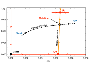
Figure 8: Template for the matching of an asymptotically safe MSSM extension with $10^{-2}\lesssim\alpha_{3}^{*}|_{\text{UV}}\lesssim\alpha_{3}^{*}|_{\text{IR}}$ to the SM at low energies (layout as in Fig. 7). Notice that the SM running dictates the bound (89) for the strong gauge coupling in the UV.

D Standard Hierarchy

Given the result (87), we now discuss prospects for MSSM extensions with UV fixed points where $\delta\alpha_{2}$ perturbations can be matched to the SM. It either requires lower values for $\alpha_{3}$ in the UV, or a tilt of the UV-IR connecting separatrix, or a combination of both.

The first scenario is illustrated in Fig. 8, where the black dashed line shows the SM running of couplings between the TeV and the Planck scale. Here, we assume that the standard hierarchy

$$\alpha^{*}_{3}|_{\rm UV}<\alpha^{*}_{3}|_{\rm IR}$$ (88)

is observed. Unlike in the benchmark model, however, we speculate that the fixed point coupling $\alpha^{*}_{3}$ is small enough to allow for a matching at TeV energies or above. More specifically, this would require that the gauge coupling fixed point sits within the range

$$0.001\lesssim\alpha_{3}^{*}\big{|}_{\rm UV}\lesssim 0.01\,,$$ (89)

and is smaller by at least one order of magnitude than what has been found in our models, see (77). To leading order in perturbation theory, we have observed the bound (61) for all our models. This technical constraint may be overcome at higher loop order, or non-perturbatively.

E Inverted Hierarchy

The second scenario questions the robustness of the hierarchy (88). Assuming that MSSM extensions can be found where the converse holds true,

$$\alpha^{*}_{3}|_{\rm UV}>\alpha^{*}_{3}|_{\rm IR}\,,$$ (90)

a matching to the SM would become a possibility owing to a “tilted” separatrix (Fig. 9) . Consequently, the separatrix may cross the SM line in the energy range where $\alpha_{3}$ is small.

Figure 9: Template for the matching of an asymptotically safe MSSM extension with $10^{-2}\ll\alpha_{3}^{*}|_{\text{UV}}$ to the SM at low energies (layout as in Fig. 7). A successful matching requires $\alpha_{3}^{*}|_{\text{IR}}\lesssim\alpha_{3}^{*}|_{\text{UV}}$ and a tilted separatrix in comparison to Fig. 8.

To check the feasibility of this in perturbation theory, we look into the general expressions for fixed points (25), (29) and (30) in terms of loop coefficients. After re-arranging terms, we find that the UV and IR fixed points are related as

$$\alpha_{3}^{*}\big{|}_{\text{IR}}=\alpha_{3}^{*}\big{|}_{\text{UV}}-\frac{C^{\prime}_{32}}{C^{\prime}_{33}}\,\alpha_{2}^{*}\big{|}_{\text{IR}}\,.$$ (91)

Hence, an inverted hierarchy requires $C^{\prime}_{32}/C^{\prime}_{33}>0$. For sufficiently small one-loop factor $B_{a}$, the diagonal entries $C^{\prime}_{aa}$ are always positive in any QFT, though they may become negative for larger positive $B_{a}$, while the off-diagonal terms $C^{\prime}_{ab}$ $(a\neq b)$ may have either sign for general $B_{a}$. Further, (23) together with the mandatory sign flip (27), (28) requires a negative $C^{\prime}_{23}<0$. Altogether, the necessary and sufficient conditions for an inverted hierarchy are

$$B_{2} <0\,,$$ (92)

$$B_{3}\,C^{\prime}_{23} <B_{2}\,C^{\prime}_{33}\,,$$

$$B_{2}\,C_{22}^{\prime} <B_{3}\,C^{\prime}_{32}\,,$$

$$0 <B_{3},C^{\prime}_{32},C^{\prime}_{33}\,.$$

They imply that the Yukawa-shifted off-diagonal two-loop coefficients must have opposite signs,

$$C^{\prime}_{23}<0<C^{\prime}_{32}\,.$$ (93)

Next, we check the conditions (93), and hence (92) for extensions of the MSSM with superpotentials $W$ involving quark singlets $\overline{q}$, quark doublets $Q$, lepton doublets $L$, and gauge singlets $S$, which we write schematically as

$$W\supset y_{i}(\overline{q}QL),\;y_{i}(S\overline{Q}Q)\;,$$ (94)

and where the index $i$ counts the different Yukawa terms. The gauge beta functions (18) are characterised by the two-loop matrix $C$,

$$C=\left(\begin{array}[]{c|c}\\ 7\sum\limits_{\text{SU}(2)}d_{3}(R)-48&16\sum\limits_{\text{SU}(3)\otimes\text{SU}(2)}1\\[17.22217pt] \hline\cr\\ 6\sum\limits_{\text{SU}(3)\otimes\text{SU}(2)}1&\;\;\frac{34}{3}\sum\limits_{\text{SU}(3)}d_{2}(R)-108\\ \end{array}\right)$$ (99)

where the sums account for the MSSM and BSM fields charged under the SM gauge groups with dimension $d_{2,3}(R)$. The off-diagonal entries, which are positive as in any quantum field theory, obey

$$C_{32}=\mbox{\small{$\frac{3}{8}$}}\,C_{23}\,.$$ (100)

Turning to the Yukawas, they contribute to the running of the gauge couplings with coefficients $D_{3i}=8$ and $D_{2i}=12$. The Yukawa beta functions (16) are characterised by the one-loop matrix $E$ (which we do not need to specify explicitly), and by the gauge contributions $F_{i3}=\frac{32}{3}$ and $F_{i2}=6$. The latter are known explicitly because the superpotential (94) has exactly two superfields in the fundamental representation of either $\text{SU}(3)_{C}$ and $\text{SU}(2)_{L}$. From (16), and in terms of (2) and (15) we find the Yukawa nullclines

$$\alpha_{i}=(\mbox{\small{$\frac{32}{3}$}}\alpha_{3}+6\alpha_{2})\sum\limits_{j}(E^{-1})_{ij}\,.$$ (101)

Note that while the matrix elements of $E$ are always positive, this does not need to hold true a priori for those of $E^{-1}$. However, for quantum field theories with physical perturbative fixed points, the sums $\sum_{j}(E^{-1})_{ij}$ must all be positive to ensure positivity for all squared Yukawa couplings $\alpha_{i}$ (we have checked explicitly that this is true for all models studied here). Consequently, we find the Yukawa-shifted two-loop matrix (22) as

$$C^{\prime}=C-\left(\begin{array}[]{ccc}72&&128\\ 48&&\frac{256}{3}\end{array}\right)\sum\limits_{ij}(E^{-1})_{ij}\,.$$ (102)

To test (93) we focus on the off-diagonal elements, which may take either sign. Most notably, the relation (100) continues to hold true for the matrix $C^{\prime}$ where Yukawa-induced shifts have been taken into account,

$$C^{\prime}_{32}=\mbox{\small{$\frac{3}{8}$}}\,C^{\prime}_{23}\,.$$ (103)

Thus, the condition (93), and hence (92), cannot be satisfied for any of the models involving the MSSM with additional quark singlets $\overline{q}$, quark doublets $Q$, and lepton doublets $L$ and superpotential (94) (In App.F we show that the result generalises for superfields in general representations.) We conclude that the hierarchy (88) is a rather robust feature of models and that scenarios with $\mu_{\rm SM}\gtrsim{\cal O}(1\,{\rm TeV})$ require either superpotentials different from those studied here, higher order loop corrections, or non-perturbative effects. We plan to explore these possibilities elsewhere.

V Discussion and Concluding Remarks

Motivated by the recent discovery of interacting ultraviolet fixed points in weakly-coupled supersymmetric theories Bond:2017suy , we have performed a comprehensive search for fixed points and asymptotic safety in extensions of the minimally supersymmetric Standard Model involving either new quark singlets, new quark doublets, or a fourth generation. We thereby have performed a scan over about 200k different MSSM extensions, most of which show infrared conformal fixed points (Figs. 2, 4 and 5), and about a hundred candidates with ultraviolet ones (Figs. 2, 3). All settings predict low-scale supersymmetry-breaking and a violation of $R$-parity.

While interacting fixed points can arise prolifically in asymptotically free gauge theories, here, we observe that their occurrence is much more constrained due the loss of asymptotic freedom in the weak gauge sector. The latter is an unavoidable consequence of supersymmetry, following from the already known charge carriers of the Standard Model. We expect that the availability of interacting fixed points will be equally constrained in other supersymmetric extensions including string-inspired models with many vectorlike representations, or supersymmetric grand unified theories.

By and large, in all models the fixed point couplings (61), (68), (75) are found to be small. Enhancing the number of independent superpotential couplings tends to enhance the values of fixed point couplings (Figs. 2, 3, 4 and  5). Thus, a reduction of flavor symmetry effectively requires stronger gauge interactions to achieve conformality. In some settings couplings may become borderline perturbative (Figs. 2, 6), which calls for higher loop studies Novikov:1983uc ; Novikov:1985rd or non-perturbative checks Intriligator:2003jj ; HLM22 . We further noticed that models with interacting UV fixed points always also display an interacting IR fixed point Bond:2017suy , while the converse is not the case. All our results are consistent with formal constraints such as the $a$-theorem, positivity of central charges, the conformal collider bound, and bounds from unitarity Cardy:1988cwa ; Osborn:1989td ; Anselmi:1997am ; Hofman:2008ar ; Komargodski:2011vj .

From a phenomenological perspective, the fixed point candidates in Tab. 4 are of interest as they may lead to ultraviolet completions of the Standard Model. Supersymmetry enhances the predictive power of interacting fixed points over non-interacting ones, leading to a smaller number of fundamentally free parameters. However, although fixed points can be matched to the Standard Model (Fig. 7) and the intrinsic $R$-parity violation can be tuned to stay within experimental bounds Dawson:1985vr ; Barbieri:1985ty ; Barger:1989rk ; Godbole:1992fb ; Bhattacharyya:1995pq ; Dreiner:1997uz ; Domingo:2018qfg , the matching scale comes out too low (87). The reason for this null result is that the strong gauge coupling $\alpha_{3}^{*}$ in the UV is simply not small enough, and that it grows along trajectories leaving the fixed point. Settings with fixed point couplings in the range (86), (89) can alleviate this impasse (Fig. 8), as can extensions where the UV-safe separatrix is tilted towards smaller couplings (Fig. 9). Either of these options require higher loops, non-perturbative effects, or interactions beyond those considered here. We have not been concerned with the $U(1)_{Y}$ sector which remains infrared free despite of interacting fixed points. This is viable phenomenologically because the $U(1)_{Y}$ Landau pole arises beyond the Planck scale for most of the fixed point scenarios discussed here. Still, it will be worth investigating whether MSSM extensions can also stabilise $U(1)_{Y}$.

A perhaps unexpected aspect of partially interacting UV fixed points is that the running of relevant perturbations may still be only logarithmic (83), (85) as in asymptotic freedom Bond:2017suy , rather than power-law. This feature percolates to the running of other parameters such as soft supersymmetry breaking terms, or gaugino masses. Therefore, and much unlike fully interacting UV fixed points in non-supersymmetric theories Litim:2014uca ; Bond:2017lnq , relevant supersymmetric perturbations would only show power-law running if at least one of the asymptotically nonfree gauge couplings remains interacting in the UV (meaning UV fixed points with $\alpha_{2}^{*},\alpha_{3}^{*}>0$ in our models). If this scenario is realised, gaugino masses will exhibit power-law running with scale, and may offer a possible solution to the supersymmetric flavor problem Martin:2000cr . Future work should clarify if this scenario can arise for semi-simple supersymmetric matter-gauge theories, because if it does, it may open up yet another route to UV-complete the Standard Model.

Acknowledgements.— This work is supported by the Science and Technology Facilities Council (STFC) under the Consolidated Grant ST/T00102X/1 (DL).

Appendices

A Yukawa nullclines

In this appendix, we have a look into Yukawa nullclines, motivated by the observation that the one loop beta functions of certain Yukawa couplings may not come out proportional to the Yukawa couplings themself, but, instead, be driven by inhomogeneous terms. Consider, for example, a model with the superpotential

$$W=y_{1}ABC+y_{2}ABD+y_{3}AEC+y_{4}AED,$$ (104)

involving chiral superfields $A,B,C,D$, and $E$. The one-loop Feynman diagram

(105)

contributes to the running of $y_{1}$ and yields a contribution $\propto y_{2}\,y_{4}^{*}\,y_{3}$. Hence, the coupling $y_{1}$ would seem unnatural tHooft:1979rat in that it can be switched on by fluctuations, as long as the other Yukawas are non-zero. Specifically, the system of Yukawa beta functions for the superpotential (104) reads

$$\begin{aligned} \beta_{y_{1}}&=y_{1}(3|y_{1}|^{2}+3|y_{2}|^{2}+|y_{3}|^{2}-A_{1})+y_{2}y_{4}^{*}y_{3}\,,\\ \beta_{y_{2}}&=y_{2}(3|y_{2}|^{2}+3|y_{1}|^{2}+|y_{4}|^{2}-A_{2})+y_{1}y_{3}^{*}y_{4}\,,\\ \beta_{y_{3}}&=y_{3}(3|y_{3}|^{2}+3|y_{4}|^{2}+|y_{1}|^{2}-A_{3})+y_{4}y_{2}^{*}y_{1}\,,\\ \beta_{y_{4}}&=y_{4}(3|y_{4}|^{2}+3|y_{3}|^{2}+|y_{2}|^{2}-A_{4})+y_{3}y_{1}^{*}y_{2}\,,\end{aligned}$$ (106)

where we absorbed the loop factor $4\pi$ into the couplings. The coefficients $A_{i}=A_{i}(g^{2})$ are positive and linear functions of the gauge coupling squares $g^{2}$ Bond:2016dvk . The Yukawa nullclines are found by solving $\beta_{y_{i}}=0$ in (106) for the Yukawas. In the absence of inhomogeneous terms, the nullcline conditions are linear functions of $|y_{i}|^{2}$. In the presence of inhomogeneous terms, the nullcline conditions become cubic functions of $y_{i}$. Note that enhanced symmetry, for instance $y_{1}=y_{2}=y_{3}=y_{4}$ in  (106), also lead to linear nullcline conditions.

In this work, we limit ourselves to superpotentials with linear nullcline conditions. In practice, this is achieved by permutation symmetries (as seen above), or by selecting superpotentials where any two trilinear terms have at most one superfield in common.

B Expressions for Fixed Points

General expressions for the partially interacting fixed points $\text{FP}_{3}$ and $\text{FP}_{23}$ have been given in the main text, see (24), (25), and (29), (30), respectively. Here, we provide formal expressions for the fixed point candidates $\text{FP}_{13}$ and $\text{FP}_{123}$ in terms of loop coefficients. For the fixed point $\text{FP}_{13}$, we have

$$\begin{aligned} \alpha_{3}^{*}\big{|}_{\text{FP}_{13}}&=\frac{B_{3}C_{11}^{\prime}-B_{1}C_{31}^{\prime}}{C_{11}^{\prime}C_{33}^{\prime}-C_{13}^{\prime}C_{31}^{\prime}}\;,\;\\ \alpha_{2}^{*}\big{|}_{\text{FP}_{13}}&=0\;,\;\\ \alpha_{1}^{*}\big{|}_{\text{FP}_{13}}&=\frac{B_{1}C_{33}^{\prime}-B_{3}C_{13}^{\prime}}{C_{11}^{\prime}C_{33}^{\prime}-C_{13}^{\prime}C_{31}^{\prime}}\;,\end{aligned}$$ (107)

while for $\text{FP}_{123}$, the expressions read

$$\begin{aligned} \alpha_{3}^{*}\big{|}_{\text{FP}_{123}}&=\frac{B_{3}(C_{12}^{\prime}C_{21}^{\prime}-C_{11}^{\prime}C_{22}^{\prime})-B_{1}(C_{21}^{\prime}C_{32}^{\prime}-C_{22}^{\prime}C_{31}^{\prime})-B_{2}(C_{12}^{\prime}C_{31}^{\prime}-C_{11}^{\prime}C_{32}^{\prime})}{C_{12}^{\prime}C_{21}^{\prime}C_{33}^{\prime}-C_{12}^{\prime}C_{23}^{\prime}C_{31}^{\prime}-C_{13}^{\prime}C_{21}^{\prime}C_{32}^{\prime}+C_{13}^{\prime}C_{22}^{\prime}C_{31}^{\prime}+C_{11}^{\prime}C_{23}^{\prime}C_{32}^{\prime}-C_{11}^{\prime}C_{22}^{\prime}C_{33}^{\prime}}\;,\;\\ \alpha_{2}^{*}\big{|}_{\text{FP}_{123}}&=\frac{B_{1}(C_{21}^{\prime}C_{33}^{\prime}-C_{23}^{\prime}C_{31}^{\prime})+B_{2}(C_{13}^{\prime}C_{31}^{\prime}-C_{11}^{\prime}C_{33}^{\prime})-B_{3}(C_{13}^{\prime}C_{21}^{\prime}-C_{11}^{\prime}C_{23}^{\prime})}{C_{12}^{\prime}C_{21}^{\prime}C_{33}^{\prime}-C_{12}^{\prime}C_{23}^{\prime}C_{31}^{\prime}-C_{13}^{\prime}C_{21}^{\prime}C_{32}^{\prime}+C_{13}^{\prime}C_{22}^{\prime}C_{31}^{\prime}+C_{11}^{\prime}C_{23}^{\prime}C_{32}^{\prime}-C_{11}^{\prime}C_{22}^{\prime}C_{33}^{\prime}}\;,\;\\ \alpha_{1}^{*}\big{|}_{\text{FP}_{123}}&=\frac{B_{1}(C_{23}^{\prime}C_{32}^{\prime}-C_{22}^{\prime}C_{33}^{\prime})+B_{2}(C_{12}^{\prime}C_{33}^{\prime}-C_{13}^{\prime}C_{32}^{\prime})-B_{3}(C_{12}^{\prime}C_{23}^{\prime}-C_{13}^{\prime}C_{22}^{\prime})}{C_{12}^{\prime}C_{21}^{\prime}C_{33}^{\prime}-C_{12}^{\prime}C_{23}^{\prime}C_{31}^{\prime}-C_{13}^{\prime}C_{21}^{\prime}C_{32}^{\prime}+C_{13}^{\prime}C_{22}^{\prime}C_{31}^{\prime}+C_{11}^{\prime}C_{23}^{\prime}C_{32}^{\prime}-C_{11}^{\prime}C_{22}^{\prime}C_{33}^{\prime}}\;.\end{aligned}$$ (108)

We emphasize that none of the studied models features a physical fixed point candidate of the type $\text{FP}_{1}$, $\text{FP}_{12}$, $\text{FP}_{13}$ or $\text{FP}_{123}$ with all couplings positive.
When interacting fixed point may exist, i.e., for $N_{q,{\rm BSM}}\leq 4$, see Sec. C, we can state a general lower bound on $\alpha_{3}^{*}\big{|}_{\text{FP}_{3}}=B_{3}/C^{\prime}_{33}$. From (22) it is clear that $C^{\prime}_{33}<C_{33}$ and with the expressions of App. C we can write

$$\alpha_{3}^{*}\big{|}_{\text{FP}_{3}}>\frac{6-N_{q,{\rm BSM}}}{28+\frac{34}{3}N_{q,{\rm BSM}}}>\frac{3}{110}\approx 0.027\;,$$ (109)

where $N_{q,{\rm BSM}}\leq 4$ has been used.

C Beta Functions: New Quark Singlets

Here, we summarise formulæ for the perturbative RG equations of type I of MSSM extensions introduced in Sec. D, with superpotential terms parametrised by (57). In terms of these parameters, the lower bounds on BSM matter fields (LABEL:eq:model1parameterscan) are given by

$$\begin{aligned} &n^{\text{min}}_{d}=\text{max}\{I_{12}+I_{13}+I_{d}-2\;,\;0\}\;,\\ &n^{\text{min}}_{u}=\text{max}\{I_{u}-2\;,\;0\}\;,\\ &n_{L}^{\text{min}}=\text{max}\{2(I_{12}+I_{13})+I_{d}-3\;,\;I_{u}\}\,,\end{aligned}$$ (110)

with $I_{d}=I_{1d}+I_{2d}+I_{3d}$ and $I_{u}=I_{1u}+I_{2u}+I_{3u}$. Using (15) for the reduced BSM Yukawas $(i=4,\cdots,13)$, we conclude that the RG running of all models with (57) is encoded by up to 15 different beta functions for the gauge couplings $\{\alpha_{1},\alpha_{2},\alpha_{3}\}$, and up to 12 Yukawa couplings given by the top and bottom Yukawas $\{\alpha_{t},\alpha_{b}\}$, and nine beyond MSSM Yukawas $\{\alpha_{4},\cdots,\alpha_{13}\}$, modulo additional copies due to flavor symmetries. The corresponding Yukawa beta functions are denoted as $\beta_{t},\beta_{b},\beta_{4},...,\beta_{13}$, with $\partial_{t}\alpha_{i}\equiv\beta_{i}$. The general beta functions for the Yukawa and gauge couplings are given in (16) and (18), respectively, involving the loop coefficients $B,C,D,E$ and $F$. Using the gauge couplings (2) and Yukawa couplings (15) with $\{y_{i}\}$ as in (57) the one-loop gauge coefficients $B$ read

$$B_{3} =6-2(n_{u}+n_{d})\;,\;$$ (111)

$$B_{2} =-2-2n_{L}\;,\;$$

$$B_{1} =-22-\mbox{\small{$\frac{16}{3}$}}n_{u}-\mbox{\small{$\frac{4}{3}$}}n_{d}-2n_{L}\;,$$

The two-loop matrices $C$ and $D$, and the one-loop matrices $E$ and $F$ in the Yukawa sector are given by

$$C =\left(\begin{array}[]{c|c|c}\frac{398}{9}+\frac{256}{27}n_{u}+\frac{16}{27}n_{d}+2n_{L}&\;\;18+6n_{L}&\;\frac{176}{3}+\frac{256}{9}n_{u}+\frac{64}{9}n_{d}\\[4.30554pt] \hline\cr 6+2n_{L}&50+14n_{L}&48\\[4.30554pt] \hline\cr\frac{22}{3}+\frac{32}{9}n_{u}+\frac{8}{9}n_{d}&18&28+\frac{68}{3}(n_{u}+n_{d})\\ \end{array}\right)\;,$$ (115)

$$D =\left(\setcounter{MaxMatrixCols}{12}\begin{smallmatrix}\frac{52}{3}x_{t}&\frac{28}{3}x_{b}&\frac{28}{3}I_{12}&\frac{28}{3}I_{1d}&\frac{28}{3}I_{12}&\frac{28}{3}I_{2d}&\frac{28}{3}I_{13}&\frac{28}{3}I_{13}&\frac{28}{3}I_{3d}&\frac{28}{3}I_{1u}&\frac{52}{3}I_{2u}&\frac{52}{3}I_{3u}\\[4.30554pt] 12x_{t}&12x_{b}&12I_{12}&12I_{1d}&12I_{12}&12I_{2d}&12I_{13}&12I_{13}&12I_{3d}&12I_{1u}&12I_{2u}&12I_{3u}\\[4.30554pt] 8x_{t}&8x_{b}&8I_{12}&8I_{1d}&8I_{12}&8I_{2d}&8I_{13}&8I_{13}&8I_{3d}&8I_{1u}&8I_{2u}&8I_{3u}\end{smallmatrix}\right)\;.$$ (116)

$$E {=}\left(\setcounter{MaxMatrixCols}{12}\begin{smallmatrix}{\scriptstyle 12}&2x_{b}&0&0&0&0&0&2I_{13}&2I_{3d}&0&0&2I_{3u}\\ 2x_{t}&{\scriptstyle 12}&0&0&0&0&0&2I_{13}&2I_{3d}&0&0&2I_{3u}\\ 0&0&{\scriptstyle 10{+}2I_{12}}&2I_{1d}&4&0&2I_{13}&0&0&2I_{1u}&0&0\\ 0&0&2I_{12}&{\scriptstyle 10{+}2I_{1d}}&0&0&2I_{13}&0&0&2I_{1u}&0&0\\ 0&0&4&0&{\scriptstyle 10{+}2I_{12}}&2I_{2d}&0&0&0&0&2I_{2u}&0\\ 0&0&0&0&2I_{12}&{\scriptstyle 10{+}2I_{2d}}&0&0&0&0&2I_{2u}&0\\ 0&0&2I_{12}&2I_{1d}&0&0&{\scriptstyle 10{+}2I_{13}}&4&0&2I_{1u}&0&0\\ 2x_{t}&2x_{b}&0&0&0&0&4&{\scriptstyle 10{+}2I_{13}}&2I_{3d}&0&0&2I_{3u}\\ 2x_{t}&2x_{b}&0&0&0&0&0&2I_{13}&{\scriptstyle 10{+}2I_{3d}}&0&0&2I_{3u}\\ 0&0&2I_{12}&2I_{1d}&0&0&2I_{13}&0&0&{\scriptstyle 10{+}2I_{1u}}&0&0\\ 0&0&0&0&2I_{12}&2I_{2d}&0&0&0&0&{\scriptstyle 10{+}2I_{2u}}&0\\ 2x_{t}&2x_{b}&0&0&0&0&0&2I_{13}&2I_{3d}&0&0&{\scriptstyle 10{+}2I_{3u}}\\ \end{smallmatrix}\right)\;,$$ (117)

$$F =\left(\setcounter{MaxMatrixCols}{12}\begin{smallmatrix}\frac{26}{9}&\frac{14}{9}&\frac{14}{9}&\frac{14}{9}&\frac{14}{9}&\frac{14}{9}&\frac{14}{9}&\frac{14}{9}&\frac{14}{9}&\frac{26}{9}&\frac{26}{9}&\frac{26}{9}\\[4.30554pt] 6&6&6&6&6&6&6&6&6&6&6&6\\[4.30554pt] \frac{32}{3}&\frac{32}{3}&\frac{32}{3}&\frac{32}{3}&\frac{32}{3}&\frac{32}{3}&\frac{32}{3}&\frac{32}{3}&\frac{32}{3}&\frac{32}{3}&\frac{32}{3}&\frac{32}{3}\end{smallmatrix}\right)^{\text{T}}\;.$$ (118)

D Beta Functions: New Quark Doublets

Here we summarise formulæ for the perturbative RG equations of all gauge and Yukawa couplings for type II of MSSM extensions Sec. E, up to two loop for the gauge and one loop for the Yukawa beta functions. We also give specifics for the selection of superpotential couplings (65):

• The parameters $0\leq x_{b},x_{t}\leq 1$ determine whether respectively the MSSM bottom- and top-Yukawa couplings are switched on ($x=1$) or off ($x=0$).

• The first- and second generation quark doublets $Q_{1}$ and $Q_{2}$ can appear in terms involving up- and down quark singlets $\overline{d}_{i}$, $\overline{u}_{i}$. The parameter $1\leq I_{Q}\leq 2$ indicates whether all terms containing $Q_{1}$ and quark singlets are present while $Q_{2}$ is absent ($I_{Q}=1$), or whether both doublets appear simultaneously ($I_{Q}=2$). Which quark singlets are available is determined by parameters introduced below.

• With $0\leq x_{4},\overline{x}_{4}\leq 1$, superpotential terms involving $Q_{4}$ and first- and second generation down quarks $\overline{d}_{1,2}$ ($x_{4}$) and up-quarks $\overline{u}_{1,2}$ ($\overline{x}_{4}$) are switched on ($x=1$) or off ($x=0$).

• The parameter $0\leq I_{d}\leq 2$ determines the first- and second generation down quark singlet content in the superpotential. For $I_{d}=0$, $\overline{d}_{1}$ and $\overline{d}_{2}$ are absent while for $I_{d}=1$ only $\overline{d}_{1}$ is present in terms involving the quark doublets $Q_{1}$, $Q_{2}$ and $Q_{4}$, depending on whether they are allowed according to the parameters $I_{Q}$, $x_{4}$ and $\overline{x}_{4}$. For $I_{d}=2$ the contruction is analogous to the case $I_{d}=1$ but this time all respective terms containing both $\overline{d}_{1}$ and $\overline{d}_{2}$ are present.

• With $0\leq I_{u}\leq 2$, the presence of superpotential terms analogous to $I_{d}$ in $(iv)$ is determined, but here concerning the up quark singlets $\overline{u}_{1,2}$.

• Terms containing the third generation quark singlets $\overline{d}_{3}$ and $\overline{u}_{3}$ as well as the first- and second generation quark doublets $Q_{1}$ and $Q_{2}$ are switched on and off with the parameters $x_{3},\overline{x}_{3}$. Here, $x_{3}$ determines whether such terms with $\overline{d}_{3}$ are present ($x_{3}=1$) or not ($x_{3}=0$), while $\overline{x}_{3}$ analogously is responsible for the presence of terms containing $\overline{u}_{3}$.

• Each admitted Yukawa term gets amended by a lepton $L$ or anti-lepton $\overline{L}$, with each of these appearing at most once in the superpotential. In consequence, the number of BSM leptons needs to be larger than $n_{L,\text{min}}=\text{max}\{(1+x_{4})I_{d}+x_{3}-3,(1+\overline{x}_{4})I_{u}+\overline{x}_{3}\}$.

• The presence of the $n_{S}$ Yukawa terms involving the gauge singletts $S_{i}$ are determined by the parameter $0\leq x_{S}\leq 1$. For $x_{S}=0$ these terms do not appear in the superpotential while for $x_{S}=1$ they do.

The one-loop gauge coefficients are given by $B_{3}=2\;,\;B_{2}=-14-2n_{L}\;,\;B_{1}=-\mbox{\small{$\frac{74}{3}$}}-2n_{L}\;.$ Further, the two-loop matrices $C$ and $D$, and the Yukawa matrices $E$ and $F$ as in (16) and (18) are given by

$$C =\left(\begin{array}[]{c|c|c}\frac{1358}{27}+2n_{L}&38+6n_{L}&\frac{368}{9}\\[4.30554pt] \hline\cr\frac{38}{3}+2n_{L}&134+14n_{L}&80\\[4.30554pt] \hline\cr\frac{70}{9}&30&\frac{220}{3}\\ \end{array}\right)\;,$$ (122)

$$D =\begin{pmatrix}\frac{52}{3}x_{t}&\frac{28}{3}x_{b}&\frac{28}{3}I_{d}I_{Q}&\frac{52}{3}I_{u}I_{Q}&\frac{28}{3}I_{Q}x_{3}&\frac{52}{3}I_{Q}\overline{x}_{3}&\frac{28}{3}I_{d}x_{4}&\frac{52}{3}I_{u}\overline{x}_{4}&\frac{4}{3}n_{S}x_{S}\\ 12x_{t}&12x_{b}&12I_{d}I_{Q}&12I_{u}I_{Q}&12x_{3}I_{Q}&12\overline{x}_{3}I_{Q}&12x_{4}I_{d}&12\overline{x}_{4}I_{u}&12x_{S}n_{S}\\ 8x_{t}&8x_{b}&8I_{d}I_{Q}&8I_{u}I_{Q}&8x_{3}I_{Q}&8\overline{x}_{3}I_{Q}&8x_{4}I_{d}&8\overline{x}_{4}I_{u}&8x_{S}n_{S}\\ \end{pmatrix}\;,$$ (123)

$$E =\left(\begin{smallmatrix}12&2x_{b}&0&0&0&4I_{Q}\overline{x}_{3}&0&0&0\\ 2x_{t}&12&0&0&4I_{Q}x_{3}&0&0&0&0\\ 0&0&(10{+}2I_{d})I_{Q}&2I_{u}I_{Q}&2I_{Q}x_{3}&2I_{Q}\overline{x}_{3}&4x_{4}&0&0\\ 0&0&2I_{d}I_{Q}&(10{+}2I_{u})I_{Q}&2I_{Q}x_{3}&2I_{Q}\overline{x}_{3}&0&4\overline{x}_{4}&0\\ 0&4x_{b}&2I_{d}I_{Q}&2I_{u}I_{Q}&12I_{Q}&2I_{Q}\overline{x}_{3}&0&0&0\\ 4x_{t}&0&2I_{d}I_{Q}&2I_{u}I_{Q}&2I_{Q}x_{3}&12I_{Q}&0&0&0\\ 0&0&4I_{Q}&0&0&0&10{+}2I_{d}&2I_{u}\overline{x}_{4}&2n_{S}x_{S}\\ 0&0&0&4I_{Q}&0&0&2I_{d}x_{4}&10{+}2I_{u}&2n_{S}x_{S}\\ 0&0&0&0&0&0&2I_{d}x_{4}&2I_{u}\overline{x}_{4}&16n_{S}\\ \end{smallmatrix}\right)\;,$$ (124)

$$F =\begin{pmatrix}\frac{26}{9}&\frac{14}{9}&\frac{14}{9}&\frac{26}{9}&\frac{14}{9}&\frac{26}{9}&\frac{14}{9}&\frac{26}{9}&\frac{2}{9}\\ 6&6&6&6&6&6&6&6&6\\ \frac{32}{3}&\frac{32}{3}&\frac{32}{3}&\frac{32}{3}&\frac{32}{3}&\frac{32}{3}&\frac{32}{3}&\frac{32}{3}&\frac{32}{3}\\ \end{pmatrix}^{\text{T}}\;.$$ (125)

E Beta Functions: Fourth Generation

We summarise formulæ for the perturbative RG equations of all gauge and Yukawa couplings for type III of the MSSM extensions introduced in Sec. F. The labelling of Yukawa couplings and the $I$-parameters is given by (73), with $i\neq 3$ and the top- and bottom Yukawas always present. The free parameters in (73) parameterize the superpotential as follows:

• The number of times down-quark singlets appear exactly once in the superpotentials in terms involving $Q_{1}$ (or $Q_{3}$) is denoted by $I_{1d}$ (or $I_{3d}$).

• Appearances of down-quarks in exactly two superpotential terms involving $Q_{1}$ and $Q_{2}$, or $Q_{1}$ and $Q_{3}$, or $Q_{1}$ and $Q_{4}$ are counted by the parameters $I_{12}$, $I_{13}$ and $I_{14}$, respectively.

• We let each up-quark $\overline{u}_{i}\neq\overline{u}_{3}$ appear at most once in our investigated superpotentials. Then, $I_{1u}$ counts the number of such terms additionally involving $Q_{1}$, and $I_{4u}$ those additionally involving $Q_{4}$, with $I_{1u}+I_{4u}\leq 3$.

• Each lepton doublet $L_{i}$ and each anti-lepton doublet $\overline{L}$ (both MSSM and BSM) may appear at most once. To accomodate for all Yukawa terms, the lepton number counting parameter needs to fulfill

  $$n_{L}\,\geq\,n_{L,\text{min}}$$ (126)

  with $n_{L,\text{min}}=\text{max}\{2I_{1}{+}I_{1d}{+}I_{3d}{-}4\;,I_{1u}{+}I_{4u}\}$ and $I_{1}=I_{12}{+}I_{13}{+}I_{14}$.

The one-loop gauge coefficients read $B_{3}=2\;,\;B_{2}=-6-2n_{L}\;,\;B_{1}=-\mbox{\small{$\frac{89}{3}$}}-2n_{L}\;,$ while for the two-loop matrices $C,D$, and the Yukawa matrices $E,F$, (16) and (18), we obtain

$$C =\left(\begin{array}[]{c|c|c}\frac{1574}{27}+2n_{L}&\;\;16+6n_{L}&\frac{704}{9}\\[4.30554pt] \hline\cr\frac{22}{3}+2n_{L}&71+14n_{L}&64\\[4.30554pt] \hline\cr\frac{88}{9}&24&\frac{220}{3}\end{array}\right)\;,$$ (130)

$$D =\left(\setcounter{MaxMatrixCols}{12}\begin{smallmatrix}\frac{52}{3}&\frac{28}{3}&\frac{28}{3}I_{12}&\frac{28}{3}I_{12}&\frac{28}{3}I_{13}&\frac{28}{3}I_{13}&\frac{28}{3}I_{14}&\frac{28}{3}I_{14}&\frac{28}{3}I_{1d}&\frac{28}{3}I_{32}&\frac{52}{3}I_{1u}&\frac{52}{3}I_{4u}\\[4.30554pt] 12&12&12I_{12}&12I_{12}&12I_{13}&12I_{13}&12I_{14}&12I_{14}&12I_{1d}&12I_{32}&12I_{1u}&12I_{4u}\\[4.30554pt] 8&8&8I_{12}&8I_{12}&8I_{13}&8I_{13}&8I_{14}&8I_{14}&8I_{1d}&8I_{32}&8I_{1u}&8I_{4u}\end{smallmatrix}\right)\;.$$ (131)

$$E {=}\left(\setcounter{MaxMatrixCols}{12}\begin{smallmatrix}12&2&0&0&0&2I_{13}&0&0&0&2I_{3d}&0&0\\ 2&12&0&0&0&2I_{13}&0&0&0&2I_{3d}&0&0\\ 0&0&{\scriptstyle 10{+}2I_{12}}&4&2I_{13}&0&2I_{14}&0&2I_{1d}I_{1d}&,0&2I_{1u}&0\\ 0&0&4&{\scriptstyle 10{+}2I_{12}}&0&0&0&0&0&0&0&0\\ 0&0&2I_{12}&0&{\scriptstyle 10{+}2I_{13}}&4&2I_{14}&0&2I_{1d}&0&2+I_{1u}&,0\\ 2&2&0&0&4&{\scriptstyle 10{+}2I_{13}}&0&0&0&2I_{3d}&0&0\\ 0&0&2I_{12}&0&2I_{13}&0&{\scriptstyle 10{+}2I_{14}}&4&2I_{1d}&0&2I_{1u}&0\\ 0&0&0&0&0&0&4&{\scriptstyle 10{+}2I_{14}}&0&0&0&2I_{4u}\\ 0&0&2I_{12}&0&2I_{13}&0&2I_{14}&0&{\scriptstyle 10{+}2I_{1d}}&0&2I_{1u}&0\\ 2&2&0&0&0&2I_{13}&0&0&0&{\scriptstyle 10{+}2I_{3d}}&0&0\\ 0&0&2I_{12}&0&2I_{13}&0&2I_{14}&0&2I_{1d}&0&{\scriptstyle 10{+}2I_{1u}}&0\\ 0&0&0&0&0&0&0&2I_{14}&0&0&0&{\scriptstyle 10{+}2I_{4u}}\\ \end{smallmatrix}\right)\;,$$ (132)

$$F =\left(\setcounter{MaxMatrixCols}{12}\begin{smallmatrix}\frac{26}{9}&\frac{14}{9}&\frac{14}{9}&\frac{14}{9}&\frac{14}{9}&\frac{14}{9}&\frac{14}{9}&\frac{14}{9}&\frac{14}{9}&\frac{14}{9}&\frac{26}{9}&\frac{26}{9}\\[4.30554pt] 6&6&6&6&6&6&6&6&6&6&6&6\\[4.30554pt] \frac{32}{3}&\frac{32}{3}&\frac{32}{3}&\frac{32}{3}&\frac{32}{3}&\frac{32}{3}&\frac{32}{3}&\frac{32}{3}&\frac{32}{3}&\frac{32}{3}&\frac{32}{3}&\frac{32}{3}\end{smallmatrix}\right)^{\text{T}}\;.$$ (133)

F Two-Loop Relations

In Sec. E, we have analysed a condition for a reverted hierarchy

$$\alpha_{3}^{*}|_{\text{UV}}>\alpha_{3}^{*}|_{\text{IR}}$$ (134)

to occur at two-loop order in perturbation theory, where $\alpha_{3}^{*}|_{\text{UV}}$ refers to the fixed point coupling at the partially interacting UV fixed point FP₃, and $\alpha_{3}^{*}|_{\text{IR}}$ refers to the fixed point coupling at the corresponding IR fixed point FP₂₃.

In this appendix, we study this relation in a more principled manner, starting with a semi-simple supersymmetric gauge theory with gauge group $G_{2}\times G_{3}$, coupled to matter and a superpotential involving superfields $A$, $B$, and $C$ which we write schematically as

$$W=\sum_{i}y_{i}(ABC)_{i}\;,$$ (135)

and $i$ counting the different Yukawa terms. We assume that $A$ and $B$ are charged under one of the gauge groups, and $B$ and $C$ are charged under the other. Then, from (6), we observe the ratio of off-diagonal two-loop gauge contributions $(a\neq b)$

$$\begin{aligned} \frac{C_{ab}}{C_{ba}}&=\frac{\sum\limits_{c}\frac{d_{c}}{d_{c}(R_{a})}S_{2}^{R_{a}}(c)C_{2}^{R_{b}}(c)}{\sum\limits_{c}\frac{d_{c}}{d_{c}(R_{b})}S_{2}^{R_{b}}(c)C_{2}^{R_{a}}(c)}\,.\end{aligned}$$ (136)

Here, $c$ counts all superfields simultaneously charged under the gauge groups $G_{a}$ and $G_{b}$ (without representation components), and $d_{c}$ is the product of all dimensionalities of groups under which the field counted by $c$ is charged. Using the identity $S_{2}^{R_{a}}(c)\,d(G_{a})=d_{c}(R_{a})\,C_{2}^{R_{a}}(c)$, the ratio (136) simplifies into

$$\begin{aligned} \frac{C_{ab}}{C_{ba}}&=\frac{d(G_{b})}{d(G_{a})}=\frac{N_{b}^{2}-1}{N_{a}^{2}-1}\end{aligned}$$ (137)

for $a\neq b$. We further specified to $G_{i}=\text{SU}(N_{i})$ gauge groups in the last step. Evidently, the general result (137) falls back onto (100) for $N_{2}=2$ and $N_{3}=3$, as it must.

Next, we are interested in the ratio of the off-diagonal Yukawa-shifted two-loop coefficients, which by definition (22) take the form

$$\frac{C^{\prime}_{ab}}{C^{\prime}_{ba}}=\frac{(C-DE^{-1}F)_{ab}}{(C-DE^{-1}F)_{ba}}\,.$$ (138)

Here, we assumed that the Yukawa and gauge beta functions can always be written as in (16), (18). The key observation is that for some superpotentials the off-diagonal Yukawa-induced shift terms $(DE^{-1}F)$ simplify into expressions of the form $(E^{-1})(DF)$, meaning that any dependence on the specifics of the Yukawa nullclines, encoded in the matrix $E^{-1}$, drop out in the ratio $(DE^{-1}F)_{ab}/(DE^{-1}F)_{ba}$. In our case, we are left with the loop coefficients

$$D_{ai} =\frac{4}{d(G_{a})}\sum\limits_{k}C_{2}^{R_{a}}(k)\;,$$ (139)

$$F_{ia} =4\sum\limits_{\tilde{k}}C_{2}^{R_{a}}(\tilde{k})\;,$$ (140)

where $D_{ai}$ as defined in (17) comes from the term $2Y_{4,a}$ in (4), and $F_{ia}$ comes from the second term of the anomalous dimensions (10). Both $D_{ai}$ and $F_{ia}$ are independent of the Yukawa index $i$, implying that any dependence on the structure of the Yukawa nullclines drops out,

$$\frac{(DE^{-1}F)_{ab}}{(DE^{-1}F)_{ba}}=\frac{(DF)_{ab}}{(DF)_{ba}}=\frac{d(G_{b})}{d(G_{a})}\;.$$ (141)

Hence, since the ratio of the off-diagonal elements (136) and the ratio of the shift terms (141) are identical, it follows that the shifted matrix elements (138), again, have the same ratio,

$$\frac{C_{ab}}{C_{ba}}=\frac{(DE^{-1}F)_{ab}}{(DE^{-1}F)_{ba}}=\frac{C^{\prime}_{ab}}{C^{\prime}_{ba}}\,.$$ (142)

Since $C_{ab}$ for $a\neq b$ are positive numbers in any quantum field theory, it follows that $C^{\prime}_{ab}<0<C^{\prime}_{ba}$ is strictly out of reach for these types of theories.

For other explicit examples of perturbatively controlled supersymmetric quantum field theories with interacting fixed points where the relations (137), (141), and (142) are realised in a large-$N$ Veneziano limit, we refer to the models in Bond:2017suy .

References

- (1) Particle Data Group collaboration, Review of Particle Physics, PTEP 2020 (2020) 083C01.
- (2) R. Barbieri and A. Strumia, The ’LEP paradox’, in 4th Rencontres du Vietnam: Physics at Extreme Energies (Particle Physics and Astrophysics), 7, 2000 [hep-ph/0007265].
- (3) N. Arkani-Hamed and S. Dimopoulos, Supersymmetric unification without low energy supersymmetry and signatures for fine-tuning at the LHC, JHEP 06 (2005) 073 [hep-th/0405159].
- (4) H. Baer, V. Barger, S. Salam, D. Sengupta and K. Sinha, Status of weak scale supersymmetry after LHC Run 2 and ton-scale noble liquid WIMP searches, Eur. Phys. J. ST 229 (2020) 3085 [2002.03013].
- (5) A.D. Bond and D.F. Litim, Theorems for Asymptotic Safety of Gauge Theories, Eur. Phys. J. C77 (2017) 429 [1608.00519].
- (6) A.D. Bond and D.F. Litim, Price of Asymptotic Safety, Phys. Rev. Lett. 122 (2019) 211601 [1801.08527].
- (7) D.F. Litim and F. Sannino, Asymptotic safety guaranteed, JHEP 12 (2014) 178 [1406.2337].
- (8) A.D. Bond, D.F. Litim, G. Medina Vazquez and T. Steudtner, UV conformal window for asymptotic safety, Phys. Rev. D 97 (2018) 036019 [1710.07615].
- (9) A.D. Bond, D.F. Litim and T. Steudtner, Asymptotic safety with Majorana fermions and new large equivalences, Phys. Rev. D 101 (2020) 045006 [1911.11168].
- (10) A.D. Bond, D.F. Litim and G.M. Vazquez, Conformal windows beyond asymptotic freedom, Phys. Rev. D 104 (2021) 105002 [2107.13020].
- (11) A.D. Bond and D.F. Litim, More asymptotic safety guaranteed, Phys. Rev. D 97 (2018) 085008 [1707.04217].
- (12) A.D. Bond and D.F. Litim, Asymptotic safety guaranteed in supersymmetry, Phys. Rev. Lett. 119 (2017) 211601 [1709.06953].
- (13) S. Weinberg, Ultraviolet divergences in quantum theories of gravitation, in: General Relativity: An Einstein centenary survey, Eds. Hawking, S.W., Israel, W; Cambridge University Press (1979) 790.
- (14) A.D. Bond, G. Hiller, K. Kowalska and D.F. Litim, Directions for model building from asymptotic safety, JHEP 08 (2017) 004 [1702.01727].
- (15) K. Kowalska, A. Bond, G. Hiller and D. Litim, Towards an asymptotically safe completion of the Standard Model, PoS EPS-HEP2017 (2017) 542.
- (16) S. Bißmann, G. Hiller, C. Hormigos-Feliu and D.F. Litim, Multi-lepton signatures of vector-like leptons with flavor, Eur. Phys. J. C 81 (2021) 101 [2011.12964].
- (17) G. Hiller, C. Hormigos-Feliu, D.F. Litim and T. Steudtner, Anomalous magnetic moments from asymptotic safety, Phys. Rev. D 102 (2020) 071901 [1910.14062].
- (18) G. Hiller, C. Hormigos-Feliu, D.F. Litim and T. Steudtner, Model Building from Asymptotic Safety with Higgs and Flavor Portals, Phys. Rev. D 102 (2020) 095023 [2008.08606].
- (19) R. Bause, G. Hiller, T. Höhne, D.F. Litim and T. Steudtner, B-anomalies from flavorful U(1)′ extensions, safely, Eur. Phys. J. C 82 (2022) 42 [2109.06201].
- (20) S.P. Martin and J.D. Wells, Constraints on Ultraviolet Stable Fixed Points in Supersymmetric Gauge Theories, Phys. Rev. D64 (2001) 036010 [hep-ph/0011382].
- (21) K. Intriligator and F. Sannino, Supersymmetric Asymptotic Safety is Not Guaranteed, JHEP 11 (2015) 023 [1508.07411].
- (22) M.A. Luty, J. Polchinski and R. Rattazzi, The -theorem and the Asymptotics of 4D Quantum Field Theory, JHEP 01 (2013) 152 [1204.5221].
- (23) B.C. Allanach, G. Amelino-Camelia and O. Philipsen, Infrared Fixed Point Structure Characterizing SUSY Symmetry Breaking, Phys. Lett. B 393 (1997) 349 [hep-ph/9611286].
- (24) M. Lanzagorta and G.G. Ross, Infrared Fixed Point Structure of Soft Supersymmetry Breaking Mass Terms, Phys. Lett. B 364 (1995) 163 [hep-ph/9507366].
- (25) T. Kobayashi and Y. Yamagishi, Quasiyukawa Fixed Point Due to Decoupling of SUSY Particles, Phys. Lett. B 381 (1996) 169 [hep-ph/9601374].
- (26) S. Codoban and D.I. Kazakov, Approximate Analytic Solutions of RG Equations for Yukawa and Soft Couplings in SUSY Models, Eur. Phys. J. C 13 (2000) 671 [hep-ph/9906256].
- (27) C.S. Aulakh and S.K. Garg, The New Minimal Supersymmetric GUT : Spectra, RG Analysis and Fermion Fits, Nucl. Phys. B 857 (2012) 101 [0807.0917].
- (28) S.A. Abel and B.C. Allanach, Ruling Out the MSSM at the Low Tan Beta Fixed Point, Phys. Lett. B 431 (1998) 339 [hep-ph/9803476].
- (29) C.-S. Huang, W. Liao, Q.-S. Yan and S.-H. Zhu, Renormalization Group Equations and Infrared Quasifixed Point Behaviors of Nonuniversal Soft Terms in MSSM, J. Phys. G 27 (2001) 833 [hep-ph/0008166].
- (30) R. Nevzorov, Quasifixed Point Scenarios and the Higgs Mass in the E6 Inspired Supersymmetric Models, Phys. Rev. D 89 (2014) 055010 [1309.4738].
- (31) J.A. Casas, J.R. Espinosa and H.E. Haber, The Higgs Mass in the MSSM Infrared Fixed Point Scenario, Nucl. Phys. B 526 (1998) 3 [hep-ph/9801365].
- (32) V.D. Barger, M.S. Berger, P. Ohmann and R.J.N. Phillips, Phenomenological Implications of the M(T) Rge Fixed Point for SUSY Higgs Boson Searches, Phys. Lett. B 314 (1993) 351 [hep-ph/9304295].
- (33) W.A. Bardeen, M. Carena, S. Pokorski and C.E.M. Wagner, Infrared Fixed Point Solution for the Top Quark Mass and Unification of Couplings in the MSSM, Phys. Lett. B 320 (1994) 110 [hep-ph/9309293].
- (34) M.E. Machacek and M.T. Vaughn, Two Loop Renormalization Group Equations in a General Quantum Field Theory. 1. Wave Function Renormalization, Nucl.Phys. B222 (1983) 83.
- (35) S.P. Martin and M.T. Vaughn, Two Loop Renormalization Group Equations for Soft Supersymmetry Breaking Couplings, Phys. Rev. D 50 (1994) 2282 [hep-ph/9311340].
- (36) S.P. Martin and M.T. Vaughn, Regularization Dependence of Running Couplings in Softly Broken Supersymmetry, Phys. Lett. B 318 (1993) 331 [hep-ph/9308222].
- (37) G.R. Farrar and P. Fayet, Phenomenology of the Production, Decay, and Detection of New Hadronic States Associated with Supersymmetry, Phys. Lett. B 76 (1978) 575.
- (38) H.K. Dreiner, An Introduction to Explicit R-Parity Violation, Adv. Ser. Direct. High Energy Phys. 21 (2010) 565 [hep-ph/9707435].
- (39) S. Dawson, R-Parity Breaking in Supersymmetric Theories, Nucl. Phys. B 261 (1985) 297.
- (40) R. Barbieri and A. Masiero, Supersymmetric Models with Low-Energy Baryon Number Violation, Nucl. Phys. B 267 (1986) 679.
- (41) V.D. Barger, G. Giudice and T. Han, Some New Aspects of Supersymmetry R-Parity Violating Interactions, Phys. Rev. D 40 (1989) 2987.
- (42) R.M. Godbole, P. Roy and X. Tata, Tau Signals of R-Parity Breaking at Lep-200, Nucl. Phys. B 401 (1993) 67 [hep-ph/9209251].
- (43) G. Bhattacharyya and D. Choudhury, D and Tau Decays: Placing New Bounds on R-Parity Violating Supersymmetric Coupling, Mod. Phys. Lett. A 10 (1995) 1699 [hep-ph/9503263].
- (44) F. Domingo, H.K. Dreiner, J.S. Kim, M.E. Krauss, M. Lozano and Z.S. Wang, Updating Bounds on -Parity Violating Supersymmetry from Meson Oscillation Data, JHEP 02 (2019) 066 [1810.08228].
- (45) V. Novikov, M.A. Shifman, A. Vainshtein and V.I. Zakharov, Exact Gell-Mann-Low Function of Supersymmetric Yang-Mills Theories from Instanton Calculus, Nucl. Phys. B 229 (1983) 381.
- (46) V. Novikov, M.A. Shifman, A. Vainshtein and V.I. Zakharov, The Beta Function in Supersymmetric Gauge Theories. Instantons Versus Traditional Approach, Sov. J. Nucl. Phys. 43 (1986) 294.
- (47) K.A. Intriligator and B. Wecht, The Exact superconformal R symmetry maximizes a, Nucl. Phys. B667 (2003) 183 [hep-th/0304128].
- (48) G. Hiller, D.F. Litim and K. Moch, in preparation, .
- (49) D. Anselmi, D. Freedman, M.T. Grisaru and A. Johansen, Nonperturbative Formulas for Central Functions of Supersymmetric Gauge Theories, Nucl. Phys. B 526 (1998) 543 [hep-th/9708042].
- (50) J.L. Cardy, Is There a c Theorem in Four-Dimensions?, Phys. Lett. B215 (1988) 749.
- (51) H. Osborn, Derivation of a Four-dimensional Theorem, Phys. Lett. B222 (1989) 97.
- (52) D.M. Hofman and J. Maldacena, Conformal collider physics: Energy and charge correlations, JHEP 05 (2008) 012 [0803.1467].
- (53) Z. Komargodski and A. Schwimmer, On Renormalization Group Flows in Four Dimensions, JHEP 12 (2011) 099 [1107.3987].
- (54) G. ’t Hooft, Naturalness, chiral symmetry, and spontaneous chiral symmetry breaking, NATO Sci. Ser. B 59 (1980) 135.