Introduction to The Dynamic Pickup and Delivery Problem Benchmark - ICAPS 2021 Competition

Abstract.

The Dynamic Pickup and Delivery Problem (DPDP) is an essential problem within the logistics domain. So far, research on this problem has mainly focused on using artificial data which fails to reflect the complexity of real-world problems. In this draft, we would like to introduce a new benchmark from real business scenarios as well as a simulator supporting the dynamic evaluation. The benchmark and simulator have been published and successfully supported the ICAPS 2021 Dynamic Pickup and Delivery Problem competition participated by 152 teams.

1. Introduction

Huawei, as one of the largest global communication device vendors, manufactures billions of products in hundreds of factories each year. A large amount of cargoes (including the raw materials, finished products and semi-finished products) need to be delivered among factories during the process of manufacturing. Due to the uncertainties of customers’ requirements and production processes, most delivery requirements cannot be fully decided in advance. The delivery orders, with the information including the pickup factories, delivery factories, the amount of cargoes and the time requirement, occur randomly and a fleet of homogeneous vehicles is periodically scheduled to serve these orders. Due to the large amount of deliver requests, even a small improvement of the logistics efficiency can bring significant benefits of finance. Therefore, it is of great significance to develop an efficient optimization algorithm to dispatch orders and plan the route of vehicles.

Masking historical datasets from real system is published with the simulator for algorithm development. The dataset contains 30 days of historical data, with 2000~5000 orders and 100~200 vehicles per day. An order can be served by several vehicles when its loading demand exceed the capacity of one vehicle. A simulator with result checking method is also provided to evaluate the performance of the algorithm over the planning horizon (e.g., one day). In the simulator, a day is split into several time intervals with the same duration (e.g., $T=144$ intervals and time interval $\Delta t=10\;min$). At the beginning of each time interval, the simulator will pass the latest environment information to the developed algorithm. After that, the scheduling results will be sent back to the simulator from the algorithm, to allow the simulator simulating the delivery process. The process will continuously be carried out until all orders are completed. To the best of our knowledge, this is the first set of dataset and simulator derived from real industrial scenes for the dynamic pickup and delivery problem, which enables related research more practical and efficient.

As mentioned above, to promote the research and application on real world problems, we organized the Dynamic Pickup and Delivery Problem competition at the 2021 International Conference on Automated Planning and Scheduling (ICAPS 2021 DPDP). In this competition, participants were expected to design algorithms from any perspectives (e.g., combinatorial optimization, heuristics methods, etc.) to schedule vehicles to serve orders generated dynamically which contain the demand to deliver cargoes from pickup factories to destinations. The overall objective is to minimize the overtime of orders as well as the average traveling distance of vehicles.

In Section 2, we will give detailed information for the benchmark, which contains detailed description for DPDP, the formulation and corresponding evaluation criteria of the problem, and the utilization methods of the benchmark. In Section 3, we will introduce the related work on this problem. In Section 4, a summary of ICAPS 2021 DPDP Competition is discussed.

2. Benchmark Description

2.1. Introduction to DPDP

Like information aforementioned, a large amount of cargoes need to be delivered among factories during the manufacturing, and each factory could be either pickup point or delivery point. Due to the uncertainties of customers’ requirements and production processes, most delivery requirements cannot be fully decided beforehand. The delivery orders, with the information including the pickup factories, delivery factories, the amount of cargoes and the time requirement, occur randomly and a fleet of homogeneous vehicles is periodically scheduled to serve these orders.

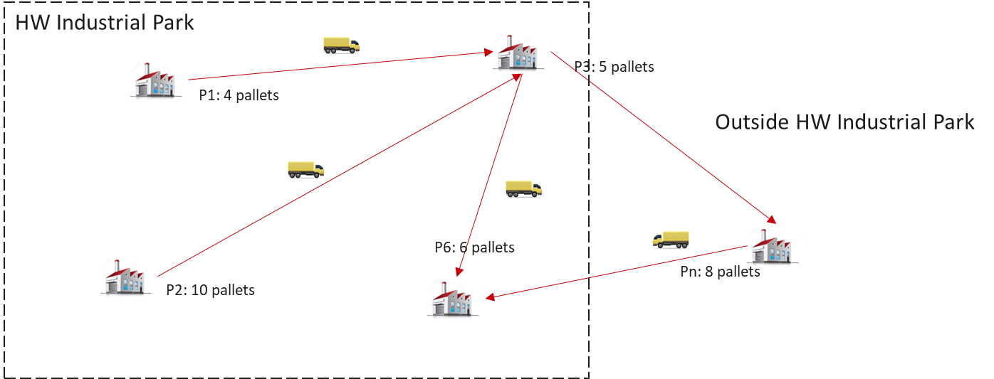
Figure 1. An Example of DPDP

Like shown in Figure 1, orders generate at factories, which contain cargoes to be sent from one factory to another. The algorithm developed should decide which vehicle is assigned to carry out this task, and also which route the vehicle should select.

2.2. DPDP Formulation and Evaluation

Generally, DPDP is formulated in several parts: input, output, constraints, and objective. Details are given below.
Input:

• A road network $G=(F,A)$, which is a complete directed graph. $F$ is the set which consists of multiple nodes (standing for factories in this competition): $\{F_{i}|i=1,\cdots,M\}$, and $A=\{(i,j)|i,j\in M\}$ is the arc set. Each arc $(i,j)$ is associated with a non-negative transportation distance $d_{ij}$ and transportation time $t_{ij}$ from node $i$ to node $j$.

• An order set $O=\{o_{i}|i=1,\cdots,N\}$, in which each order $o_{i}=(F_{p}^{i},F_{d}^{i},q^{i},t_{e}^{i},t_{l}^{i})$, where $F_{p}^{i}$ and $F_{d}^{i}$ represent the pickup and delivery node respectively, $q^{i}$ is the amount of cargoes to be delivered, which is expressed as: $q^{i}=(q_{standard}^{i},q_{small}^{i},q_{box}^{i})$, where $q_{standard}^{i}$ stands for the standard pallet amount, $q_{small}^{i}$ stands for the small pallet amount, and $q_{box}^{i}$ stands for the box amount, $t_{e}^{i}$ refers to the creation time and $t_{l}^{i}$ is the committed completion time (Note that the committed completion time refers to the competition time of each order, including the vehicle travel time, dock approaching time, dock queuing time and loading/unloading time). $1$ standard pallet equals $2$ small pallets, and $1$ small pallet equals $2$ boxes. These orders come randomly.

• A fleet of homogeneous vehicles $V=\{v_{k}|k=1,\cdots,K\}$. Each vehicle $v_{k}$ is associated with a loading capacity and work shift of drivers. The initial positions of vehicles are randomly assigned to nodes.

• $M$ nodes (factories) $\{F_{i}|i=1,\cdots,M\}$ . Each node has a limited number of cargo docks for loading and unloading, as well as work shift constraint. If all docks are in use, the newly arriving vehicles must wait for their release. And also the loading and the unloading operations can only be performed during work shift.

• Dock approaching time, the time for a vehicle between arrival at the factory and the allocation the dock without considering queuing, e.g., $30$ minutes.

• Loading and unloading time, e.g., if there are $q$ standard pallets in the vehicle, then the loading time $t_{p}=\omega\times q$ and unloading time $t_{d}=\omega\times q$,  $\omega=180\;seconds/standard\ pallet$.

Output:

• The order assignment plan and the route of each vehicle, e.g., for vehicle $v_{k}$, its route plan: $\prod_{k}=\left\{n_{1}^{k},\ n_{2}^{k},\cdots,\ n_{l_{k}}^{k}\right\}$, where $n_{i}^{k}$ is the $i$th factory the vehicle should visit.

Constraints:

• Order fulfillment. All orders need to be served.

• Committed completion time. Orders need to be completed within the committed completion time, e.g., $4$ hours. Otherwise, the penalty cost would arise.

• Order split. Splitting is only allowed for orders that exceed the vehicle’s loading capacity. The smallest unit of the order is not allowed to be divided. For example, if an order contains $13$ standard pallets, $7$ small pallets and $1$ box, the smallest units are $1$ standard pallet or $1$ small pallet or $1$ box.

• Loading capacity of the vehicle. For each vehicle $v_{k}$ , the total capacity of loaded cargoes cannot exceed the maximum loading capacity Q, e.g., $12$ standard pallets per vehicle.

• Work shift of drivers, e.g., $8:30-12:00,\ 13:30-18:00$.

• Last In First Out (LIFO) loading constraint. e.g., if orders $o_{1}$ and $o_{2}$ are assigned to the same vehicle $v_{k}$, where the pickup and delivery node of $o_{1}$ are $F_{p}^{1}$ and $F_{d}^{1}$, the pickup and delivery node of $o_{2}$ are $F_{p}^{2}$ and $F_{d}^{2}$, then the route plan $\left\{F_{p}^{1},\ F_{p}^{2},\ F_{d}^{1},\ F_{d}^{2}\right\}$ violates the LIFO constraint, while $\left\{F_{p}^{1},\ F_{p}^{2},\ F_{d}^{2},\ F_{d}^{1}\right\}$ does not.

• Limited number of cargo docks of each node: e.g., if node $F_{1}$ contains $3$ cargo docks and $4$ vehicles arrive, then the latest vehicle has to wait until one dock turns available.

• Loading and unloading is subject to the first come, first serve rule. If multiple vehicles arrive at the same node at the same time while the node has only one vacant cargo dock, then the node will randomly select one vehicle for loading and unloading. Note that the above situation will not happen in the reality, but may occur in the simulated environment.

Objectives:
This problem includes two objectives to optimize.

• The first objective is to minimize the total timeout of orders denoted as $f_{1}$:

  $$f_{1}=\sum_{i=1}^{N}\max(0,\ a_{d}^{i}-t_{l}^{i})$$

  Where $a_{d}^{i}$ and $t_{l}^{i}$ denote the arrival time to the destination and the committed completion time of order $o_{i}$ respectively, and $N$ is the total amount of orders.

• The second objective is to minimize the average traveling distance of vehicles denoted as $f_{2}$:

  $$f_{2}=\frac{1}{K}\sum_{k=1}^{K}\sum_{i=1}^{l_{k}-1}d_{n_{i}^{k},n_{i+1}^{k}}$$

  Considering that the route plan of vehicle $v_{k}$ is $\prod_{k}=\left\{n_{1}^{k},\ n_{2}^{k},\cdots,\ n_{l_{k}}^{k}\right\}$, where $l_{k}$ is the total amount of factories vehicle $v_{k}$ should visit, and $d_{n_{i}^{k},n_{i+1}^{k}}$ is the distance from node $n_{i}^{k}$ to node $n_{i+1}^{k}$

• The overall objective is acquired via:

  $$\min f=\lambda\times f_{1}+f_{2}$$

  Where $\lambda$ is a pretty large positive constant, i.e., we focus much more on the optimization of $f_{1}$

2.3. Utilization of the Benchmark

We’d like to introduce the utilization of our simulator and dataset in this part. For downloading and supplementary information for them, please access via this link: DPDP Simulator and Dataset.
Description of the Dataset:
The dataset is divided into several data types: orders, vehicles, route map, and factory information.

• Orders
  Each order file contains one day’s order information, with a file name in format ”order_count + file_number”. order_count denotes the order quantity, and file_number is used to differentiate the order data for different days. For example, file 50_1 means that this is the first file with $50$ orders per day. The order_count is ranging from $50$ to $4000$ which helps the users test their algorithm in different order quantities. The attributes in order file are explained in Table 1.

  Table 1. Description of Order Data

  Column	Description	Example
  order_id	ID of order	0003480001
  q_standard	Standard pallet amount	1
  q_small	Small pallet amount	2
  q_box	Box amount	1
  demand	Total standard pallet amount, calculated as: $q\_standard+0.5\times$ $q\_small+0.25\times q\_box$	1.75
  creation_time	Order creation time (%H:%M:%S)	00:03:48
  committed_ completion_time	Order committed completion time (%H:%M:%S)	04:03:48
  load_time	Order loading time (unit: second)	120
  unload_time	Order unloading time (unit: second)	120
  pickup_id	ID of pickup factory	2445d4bd004c457d 95957d6ecf77f759
  delivery_id	ID of delivery factory	b6dd694ae05541db a369a2a759d2c2b9

• Vehicles
  Each file contains available vehicles information, with a file name in format ”vehicle_info + vehicle_count”. vehicle_count denotes the number of vehicles available which is ranging from $5$ to $100$, make it convenient for users to test their algorithm in different vehicle quantities. The attributes are explained in Table 2.

  Table 2. Description of Vehicle Data

  Column	Description	Example
  car_num	ID of vehicle	V_1
  capacity	Capacity of vehicle (unit: standard pallet)	15
  operation_time	Operation time of vehicle (unit: hour)	24
  gps_id	ID of GPS equipment	G_1

• Route Map
  The route_map file offers the distance and travel time between each pair of factories. Details are given in Table 3.

  Table 3. Description of Route Map

  Column	Description	Example
  route_code	ID of route	e7eeb0e4-a7c7 -11eb-8344- 84a93e824626
  start_factory_id	Departure factory ID of the route	7782ed919d8f4dd6 a1fb220dacd73445
  end_factory_id	Terminal factory ID of the route	43a4215be06543c1 985c1e9460dec52d
  distance	Distance of the route (unit: km)	76.0
  time	Transportation time of the route (unit: second)	10140

• Factory Information
  The factory_info file gives the location and port (dock) information. Details are given in Table 4.

  Table 4. Description of Factory Data

  Column	Description	Example
  factory_id	ID of factory	9829a9e1f6874f28 b33b57a7a42bb49f
  longitude	Longitude of factory	116.6259
  latitude	Latitude of factory	40.2204
  port_num	Number of ports used for loading and unloading of vehicle cargoes	6

Description of the simulator:
The simulator with result checking function is provided to evaluate the performance of the algorithm over the planning horizon, e.g., one day. In the simulator, a day is split into $T$ time intervals of the same duration, e.g., $T=144$ intervals and time interval $\Delta t=10\;min$. A flowchart is given in Figure 2 for reference and the directory structure of the simulator is displayed in Figure 3.

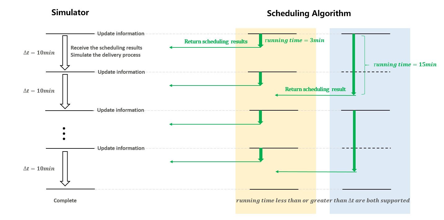
Figure 2. Interaction between the Simulator and Algorithm

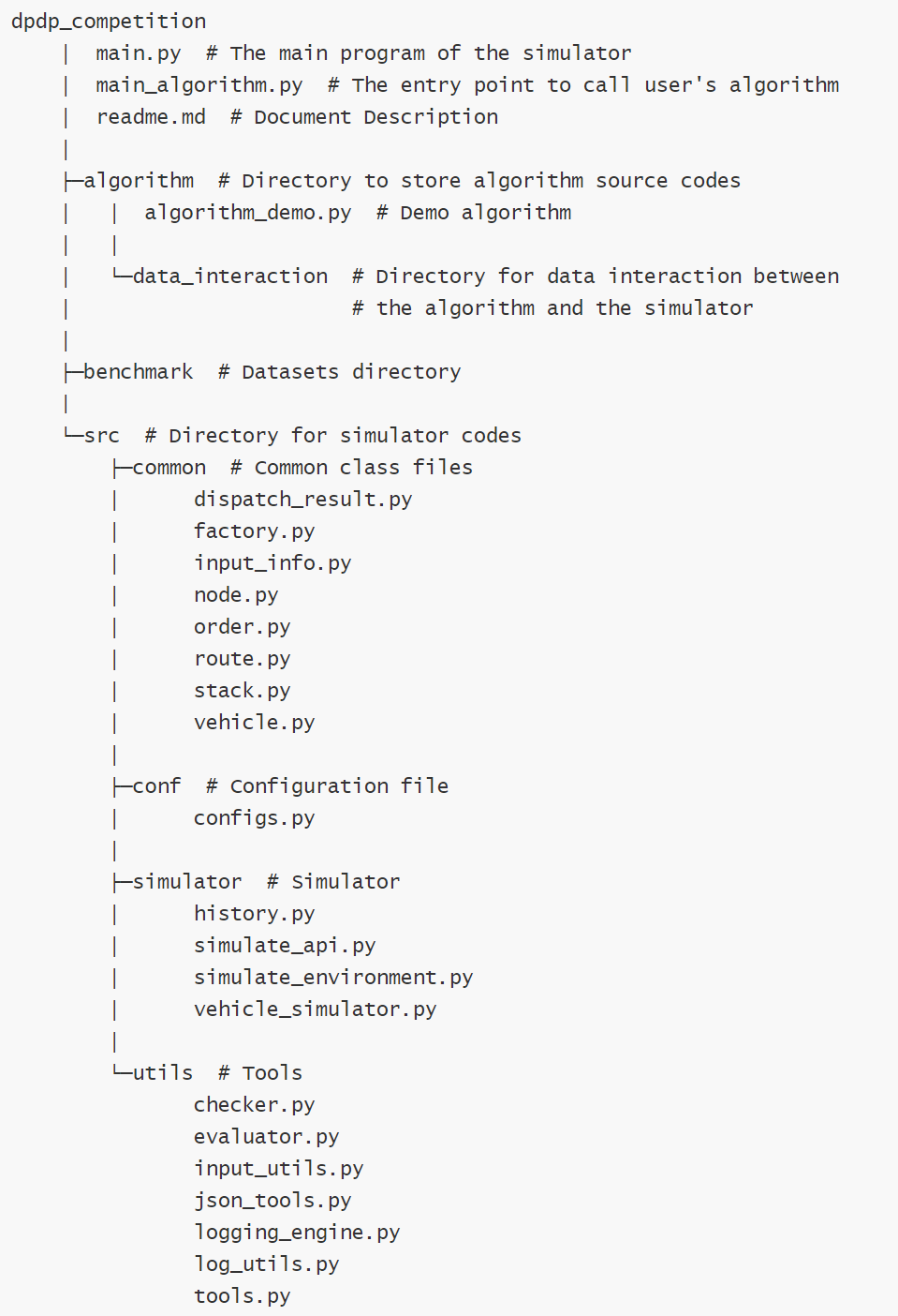
Figure 3. Directory Structure of the Simulator

Below is detailed description for utilization of the simulator from simulator perspective.

• Interaction between Algorithm and Simulator
  To start with, the simulator reads the selected test instances which can be modified in Configs.py. Then the simulator performs simulation at a fixed interval of 10 minutes until all orders in the instance are completed.
  In each round of simulation, the simulator outputs the vehicle and the order data required by the algorithm to the algorithm/data_interaction folder in JSON format. Next, it calls the main program of the algorithm prefixed with ”main_algorithm”, e.g., main_algorithm.py, main_algorithm.java, etc. When the algorithm runs, it starts to read JSON files, dispatch orders and output the dispatch result to the algorithm/data_interaction folder in JSON format and prints string ”SUCCESS” to the console as the indicator for the simulator to determine whether the algorithm is successfully executed. If the successful indicator is obtained, the simulator would read the output JSON files and do the verification. After passing the verification, it continues to simulate next round.
  The running time of the algorithm per round is limited to 10 minutes. The simulator will exit once the algorithm times out.

And below describes the interaction methods from algorithm perspective.

• Read the Input JSON Files
  The simulator outputs the latest vehicle information in vehicle_info.json, order items to be allocated in unallocated_order_items.json and ongoing order items in ongoing_order_items.json. Apparently, unallocated_order_items.json and ongoing_order_items.json have the same format. The details of these files are in Table 5 and Table 6. Some key concepts are explained here:

  • Item, which refers to the smallest indivisible unit in an order. For example, if an order contains 2 standard pallets and 1 small pallets, there are 3 individual items totally: item 1 containing one standard pallet, item 2 containing one standard pallet and item 3 containing 1 small pallet.

  • Item status 0 means initialization.

  • Item status 1 means the item is generated.

  • Item status 2 means the item has been loaded.

  • Item status 3 means the item is delivered.

  • Order status, which is the minimum value of all corresponding items statuses. For example, an order includes two items, namely, item 1 containing 1 small pallet and item 2 containing 1 box. The status of item 1 is 3 and item 2 is 2, so the overall order status is 2.
    

  Table 5. Details of vehicle_info.json

  Column	Description	Type
  id	ID of vehicle	str
  operation_time	Operation time of vehicle (unit: hour)	int
  capacity	Capacity of vehicle (unit: standard pallet)	int
  update_time	Update time of the current position and status of the vehicle (unit: Unix timestamp)	int
  cur_factory_id	Factory ID where the vehicle is currently located. Value is ”” if the vehicle is currently not in any factory.	str
  arrive_time_at_ current_factory	Time when the vehicle arrives at the current factory (unit: Unix timestamp)	int
  leave_time_at_ current_factory	Time when the vehicle leaves the current factory (unit: Unix timestamp)	int
  carrying_items	List of items loaded on the vehicle in the order of loading	[str, str,$\cdots$]
  destination	Current destination of the vehicle. Once determined, the destination cannot be changed until the vehicle has arrived. The destination is None when the vehicle is parked.	dict

  Table 6. Details of Order Items JSON File

  Column	Description	Type
  id	ID of item	str
  type	Pallet type	str
  order_id	ID of order	str
  demand	Total amount of the order in standard pallet unit	double
  pickup_factory_id	ID of pickup factory	str
  delivery_factory_id	ID of delivery factory	str
  creation_time	Creation time of the corresponding order (unit: Unix timestamp)	int
  committed_ completion_time	Committed completion time of the corresponding order (unit: Unix timestamp)	int
  load_time	Loading time of item (unit: second)	int
  unload_time	Unloading time of item (unit: second)	int
  delivery_state	Item status 0~3	int

• Dispatch Orders

  • When the vehicle $v$ arrives at the factory $f$, the pickup and delivery list of $v$ in $f$ will be generated immediately. The vehicle can only be loaded and unloaded according to the list. We can only change the pickup and delivery items of $v$ in $f$ when the corresponding pickup and delivery list is not generated.

  • Algorithm can reallocate the item to different vehicles as long as this item is not displayed on the pickup and delivery list.

  • Considering that the input is the items, the algorithm needs to pay attention to the order splitting constraint. If the order does not exceed the vehicle’s capacity (vehicles are homogeneous), the order cannot be split.

  • The algorithm can control the order release. For example, if order A is generated at $t_{1}$, the algorithm can delay the allocation until $t_{2}<=t_{1}+4h$. Note: If an order has been generated for more than 4 hours but is still not dispatched, the simulator will exit.

  • The traveling distance and time required for the algorithm can be obtained only from the distance and time matrix between factories in the benchmark. Do not calculate the distance and time based on the longitude and latitude. If the vehicle $v$ is in transit, $v$ must have a destination factory $f$, and the simulator will give the estimated time for $v$ to arrive at $f$. The algorithm can plan the route of vehicle $v$ based on the destination $f$.

  • Assume that the simulator sends the latest status information of all vehicles to the algorithm at $t_{1}$, and the algorithm returns the dispatching result at $t_{2}$. If the algorithm runs for a long time, the status of vehicles will change greatly after passing the time interval $[t_{1},t_{2}]$. As a result, the dispatching result is inconsistent with the actual situation, which affects the running of vehicles. Currently, the running time of the algorithm is limited to 10 minutes.
    

• Output Required JSON Files
  The algorithm needs to output two JSON files: output_destination.json and output_route.json. These two files have similar format, which could be explored through the readme file of the simulator. The attributes of them are explained in Table 7.

  Table 7. Attribute of Output files

  Column	Description	Type
  factory_id	ID of factory	str
  lng	Longitude of factory	double
  lat	Latitude of factory	double
  delivery_item_list	List of items unloaded from the vehicle	[str, str, $\cdots$]
  pickup_item_list	List of items loaded on the vehicle	[str, str, $\cdots$]
  arrive_time	Time to reach the factory	int
  leave_time	Time to leave the factory	int

3. Related Works

In academic aspect, DPDP is a complex variant of Vehicle Routing Problem (VRP), which has been proved to be a NP-Hard combinatorial optimization problem (Toth and Vigo, 2014). Compared to VRP, DPDP is more complex considering there are various constraints like vehicle capacity constrain, Last-In-First-Out constraint, time window constrain, split demand constraint, etc. On top of this, the orders come in a random manner which is hard to predict and acquire beforehand. There are two popular methods to solve DPDP. The first one is exact methods, which consumes too much time and doesn’t meet the need for problems at large scales (Savelsbergh and Sol, 1998). The other one is heuristic methods, which divide the problem into a series of static problems and conquer them individually (Gendreau et al., 2006; Mitrovic-Minic et al., 2004). However, a series of sub-optimal solutions don’t mean an optimal solution globally. Some methods predict the distribution of future orders to improve the solution in sub-problem (Thomas, 2007; Ghiani et al., 2009). With the development of deep learning and reinforcement learning, some researchers design learning-based methods to solve DPDP. (Ma et al., 2021) proposes a novel novel bi-level reinforcement learning agents optimization framework. The upper-level agents determines whether to release orders of the given static problem to the lower-level agent and the lower-level agent is responsible for order dis-patching and vehicle routing planning by improving an initial solution iteratively. (Li et al., 2021) designs and end-to-end reinforcement learning solution using double deep graph networks incorporating attention-based graph embedding at industrial scale.

4. Brief Summary of ICAPS 2021 Dynamic Pickup and Delivery Problem Competition

This competition was organized by Huawei Noah’s Ark Lab with Sun Yat-sen University at 2021 International Conference on Automated Planning and Scheduling. To the best of our knowledge, this competition is the first one to offer comprehensive support, from simulator, dataset to execution platform, in this field.
Totally 843 participants world-widely joined the competition and 152 teams were formed. In general, our participants used miscellaneous methods like heuristic methods, combinatorial optimization, reinforcement learning, and so on and so forth. Actually these methods are common ones often explored by both academic and industrial fields. Though in many cases heuristic methods are relatively easy to find out good acceptable solutions in a highly efficient manner, we are delighted to see there are still many participants trying in other perspectives like reinforcement learning, and we hope this could be a promising start to encourage more people to discover different aspects and core of the problem via sorts of methods.
Finally, 3 teams outperformed all other teams to win the prizes, whose algorithms utilize heuristic methods mainly. One of the awarded teams utilized Variable Neighbourhood Search method for finding out the route plans of vehicles. Generally, they continuously swap the nodes order among route plans of different vehicles and also exchange the orders inside a route plan for better result. The runner-up team develops the algorithm from the perspective of threshold check, i.e., allocating the orders by checking whether they reached the threshold of delivery time and vehicle capacity, if so, those orders would be allocated. Besides, the team also implement some trick strategies like assigning the orders to the incoming vehicles for a hitch ride. The second runner-up team sets up an additional term about docking time in the optimization goal for better regulating the time cost. They also dispatch the orders based on some specific rules like urgency rank of unallocated orders.
From the description above, one can notice that heuristic methods still dominate the problem among all kinds of algorithms, and the majority of them are bonded tightly to specific scenes, i.e., many tricky strategies are applied to fit for the problem settings. Although one kind of algorithm works well in one scene, it might fail to perform well when being transferred directly to another one. Therefore, generalization is definitely a challenging but valuable direction for algorithms development in the future. If such kind of algorithms was successfully found, even though it might not guarantee a global optimal solution, it would not only solve lots of realistic industrial problems, but could also help us understand the key points of the problem from theoretical perspective.
We have made the tech talk videos and the source codes of awarded teams publicly available, which together with other information about this competition could be found here: ICAPS 2021 DPDP Competition (ICA, 2021).
Though the competition is over, our work and effort on building an ecosystem based on DPDP have not finished yet. Recently, more and more research works have been focusing on machine learning aided optimization and scheduling algorithms. The combination of the advanced data-driven techniques and conventional solutions might bring a technique breakthrough in the near future for DPDP. To promote the research activities and industrial applications on this field incessantly, we decided to build the DPDP problem as a long-term competition at Huawei Competition Platform. Therefore, we also decided to keep the simulator and the dataset publicly available for any users who are interested in this field. We encourage any users, no matter you are from research institutes, universities or enterprises, to cite and use our simulator and dataset for improving the algorithm to solve DPDP problem. The long-term competition link can be found here: Long-term DPDP Competition (Lon, 2021).

References

- (1)
- ICA (2021) 2021. ICAPS 2021 Dynamic Pickup and Delivery Problem Competition. https://competition.huaweicloud.com/information/1000041411/introduction. (2021).
- Lon (2021) 2021. Long-term Dynamic Pickup and Delivery Problem Competition. https://competition.huaweicloud.com/information/1000041601/introduction. (2021).
- Gendreau et al. (2006) Michel Gendreau, Francois Guertin, Jean-Yves Potvin, and René Séguin. 2006. Neighborhood search heuristics for a dynamic vehicle dispatching problem with pick-ups and deliveries. Transportation Research Part C: Emerging Technologies 14, 3 (2006), 157–174.
- Ghiani et al. (2009) Gianpaolo Ghiani, Emanuele Manni, Antonella Quaranta, and Chefi Triki. 2009. Anticipatory algorithms for same-day courier dispatching. Transportation Research Part E: Logistics and Transportation Review 45, 1 (2009), 96–106.
- Li et al. (2021) Xijun Li, Weilin Luo, Mingxuan Yuan, Jun Wang, Jiawen Lu, Jie Wang, Jinhu Lu, and Jia Zeng. 2021. Learning to Optimize Industry-Scale Dynamic Pickup and Delivery Problems. (2021). arXiv:cs.AI/2105.12899
- Ma et al. (2021) Yi Ma, Xiaotian Hao, Jianye HAO, Jiawen Lu, Xing Liu, Xialiang Tong, Mingxuan Yuan, Zhigang Li, Jie Tang, and Zhaopeng Meng. 2021. A Hierarchical Reinforcement Learning Based Optimization Framework for Large-scale Dynamic Pickup and Delivery Problems. https://openreview.net/forum?id=2F_wnaioS6. In Thirty-Fifth Conference on Neural Information Processing Systems.
- Mitrovic-Minic et al. (2004) Snezana Mitrovic-Minic, Ramesh Krishnamurti, Gilbert Laporte, et al. 2004. Double-horizon based heuristics for the dynamic pickup and delivery problem with time windows. Transportation Research Part B: Methodological 38, 8 (2004), 669–685.
- Savelsbergh and Sol (1998) Martin Savelsbergh and Marc Sol. 1998. Drive: Dynamic routing of independent vehicles. Operations Research 46, 4 (1998), 474–490.
- Thomas (2007) Barrett W Thomas. 2007. Waiting strategies for anticipating service requests from known customer locations. Transportation Science 41, 3 (2007), 319–331.
- Toth and Vigo (2014) Paolo Toth and Daniele Vigo. 2014. Vehicle routing: problems, methods, and applications. SIAM.