A transiting, temperate mini-Neptune orbiting the M dwarf TOI-1759 unveiled by TESS

Abstract

We report the discovery and characterization of TOI-1759 b, a temperate (400 K) sub-Neptune-sized exoplanet orbiting the M dwarf TOI-1759 (TIC 408636441). TOI-1759 b was observed by TESS to transit on sectors 16, 17 and 24, with only one transit observed per sector, creating an ambiguity on the orbital period of the planet candidate. Ground-based photometric observations, combined with radial-velocity measurements obtained with the CARMENES spectrograph, confirm an actual period of $18.85019\pm 0.00014$ d. A joint analysis of all available photometry and radial velocities reveal a radius of $3.17\pm 0.10\,R_{\oplus}$ and a mass of $10.8\pm 1.5\,M_{\oplus}$. Combining this with the stellar properties derived for TOI-1759 ($R_{\star}=0.597\pm 0.015\,R_{\odot}$; $M_{\star}=0.606\pm 0.020\,M_{\odot}$; $T_{\textrm{eff}}=4065\pm 51$ K), we compute a transmission spectroscopic metric (TSM) value of over 80 for the planet, making it a good target for transmission spectroscopy studies. TOI-1759 b is among the top five temperate, small exoplanets ($T_{\textrm{eq}}<500$ K, $R_{p}<4\,R_{\oplus}$) with the highest TSM discovered to date. Two additional signals with periods of 80 d and $>$ 200 d seem to be present in our radial velocities. While our data suggest both could arise from stellar activity, the later signal’s source and periodicity are hard to pinpoint given the $\sim 200$ d baseline of our radial-velocity campaign with CARMENES. Longer baseline radial-velocity campaigns should be performed in order to unveil the true nature of this long period signal.

1 Introduction

One of the most exciting astronomical developments in the last decade, triggered by improved instrumentation and survey designs, is the detection and characterization of small ($R_{p}<4\,R_{\oplus}$) exoplanets. The study of transiting, relatively low-temperature small worlds, in particular, promises to provide key information to understand how different environments (e.g. incident stellar fluxes or initial composition) might impact on their bulk properties, and how those might in turn change their atmospheric and interior structures (Dorn et al., 2017; Neil & Rogers, 2020; Ma & Ghosh, 2021). In addition, these cooler worlds allow us to make connections with the planets in our own Solar System, all of which have equilibrium temperatures smaller than $500$ K (hereon referred to as “temperate” exoplanets). These connections, in turn, have key implications for the search for life outside the Solar System, and have the potential to help us improve and refine the concept of planetary habitability itself (Tasker et al., 2017; Meadows & Barnes, 2018; Seager et al., 2021).

Detecting these small, temperate exoplanets is, however, challenging. The relatively longer orbital periods needed to have small irradiation levels makes them difficult to detect from the ground using the transit technique, which is why most of the known temperate worlds were detected by the transit survey with the longest continuous time-baseline: the Kepler mission (Borucki et al., 2010). While revolutionary in the search and discovery of small worlds — revealing that they are, in fact, among the most abundant population of exoplanets in our galaxy (at least for close-in exoplanets; Fulton & Petigura, 2018; Hsu et al., 2019) — the mission provided few systems amenable for further radial-velocity and/or atmospheric characterization, due to the inherent faintness of the stars it surveyed. This detailed characterization is fundamental to understand the overall make-up of these small, distant worlds, and help us understand and uncover their different sub-populations (see, e.g. Zeng et al., 2019; Gupta & Schlichting, 2021; Schlichting & Young, 2021; Yu et al., 2021). It is also important to understand fundamental exoplanet demographic questions such as why these small worlds are the most numerous in our galaxy (see, e.g. Kite et al., 2019).

The Transiting Exoplanet Survey Satellite (Ricker et al., 2015, TESS) has been crucial to the search for small transiting exoplanets amenable for detailed characterization. To date, it has already doubled the known sample of small, temperate worlds for which masses have been measured with follow-up observations. And after three years of operation, the mission is just starting to exploit its long-time baselines, allowing the discovery of exoplanets on long orbital periods. In this work, we present the detection and characterization of one such system: TOI-1759 b, an 18.85-day sub-Neptune ($R_{p}=3.14\,R_{\oplus}$, $M_{p}=10.8\,M_{\oplus}$), orbiting a M dwarf star.

This paper is structured as follows. In § 2 we describe the data that was obtained to understand this new exoplanetary system, which includes photometric, spectroscopic and high-resolution imaging data. In § 3 we present the analysis of these data, including the stellar and planetary properties of the system. We discuss our results in § 4, and summarize our main conclusions from this work in § 5.

2 Observations

2.1 TESS

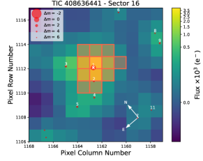
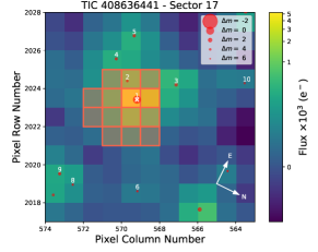
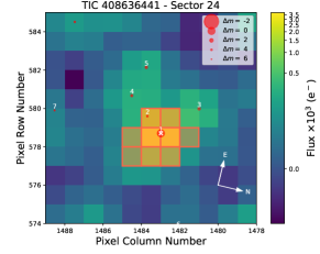
Figure 1: TESS target pixel files (TPFs) for TOI-1759 from the different sectors from which data were gathered with the mission (Sector 16 left; 17 center; 24, right). TOI-1759 is marked with a white cross on top of a red point, and is numbered as 1. Smaller numbered red points are the closest stars to the target (drawn from Gaia) with Gaia magnitude differences with the target of $|\Delta G|<6$ mag. Contamination is not a problem for TOI-1759, as most nearby targets are very faint. Plot made using tpfplotter (Aller et al., 2020).

Observations from TESS for TOI-1759 (TYC 4266-736-1, TIC408636441) were obtained during its second year of operation in its high-cadence, 2-minute exposure mode on Sectors 16 (September to October, 2019), 17 (October to November, 2019) and 24 (April to May, 2020 — see Figure 1 and 2; the data are also presented in Table 6.).

The 2-minute cadence data were processed in the TESS Science Processing Operations Center (SPOC; Jenkins et al., 2016) photometry and transit search pipelines (Jenkins, 2002; Jenkins et al., 2010) at NASA Ames Research Center. The TESS data validation reports (Twicken et al., 2018; Li et al., 2019) on TOI-1759 (Guerrero et al., 2021) show detections of a transiting exoplanet candidate at a 37.7 day period (although the data were also consistent with a planet at half this period, i.e. 18.85 days) and a transit depth of about 2700 ppm. To perform further analyses on this target, we retrieved the Pre-Data-Conditioning (PDC)-corrected photometry (Stumpe et al., 2012, 2014; Smith et al., 2012) from all sectors from the Mikulski Archive for Space Telescopes (MAST) archive, as this is the highest quality photometry from the three TESS sectors mentioned above. After removing the transits of the planet candidate, we ran the Transit Least Squares (TLS; Hippke & Heller, 2019) algorithm on these photometric time series and found no extra significant signals (i.e., signals with a signal-to-noose ratio $>$ 5) in the data.

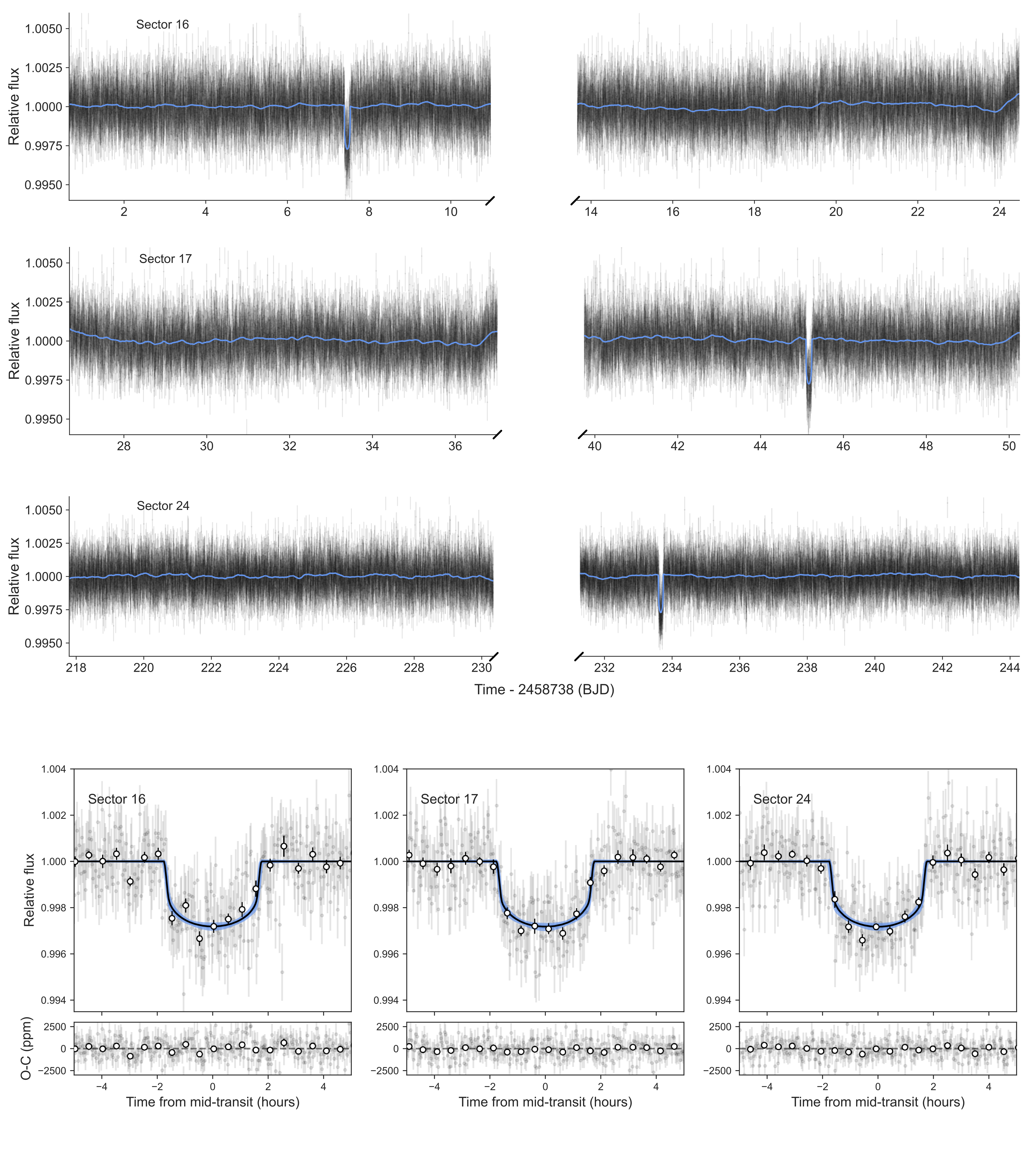
Figure 2: TESS transits of TOI-1759 b. The top panels present the TESS photometry of TOI-1759 in Sectors 16, 17 and 24 as a function of time (black points with errorbars), along with the best-fit model which consists of a transit model plus a Gaussian process (blue curve). Note there is only a single transit observed in each sector. The bottom panels shows a close-up to each of those transits, which have been phased around the time-of-mid transit (grey points with errorbars); the Gaussian process component has been removed from this photometry. The black line in these panels show the best-fit transit model; blue bands represent the 68% and 95% credibility bands of the model.

2.2 Spectroscopy

2.2.1 CARMENES

We monitored TOI-1759 with the CARMENES instrument located at the 3.5 m telescope at the Calar Alto Observatory in Almería, Spain, from July 24, 2020 to January 17, 2021. Our data covered a time span of about 175 d, over which we were able to detect significant radial-velocity signals. The spectra were processed following the standard CARMENES data flow (Caballero et al., 2016) that has been extensively used by previous works (e.g. Zechmeister et al., 2018; Morales et al., 2019; Trifonov et al., 2020). In our analyses, we only used radial-velocities from the visual (VIS) channel which had mean errors of 2.6 m/s. A total of 57 radial-velocity datapoints were used for our analysis, which are presented in Table 5. The spectra used to derive those have a median signal-to-noise ratio of 95 at 840 nm. Data from our infrared channel was not used as their precision (mean error of 10 m/s) was not enough to put meaningful constraints on the radial-velocity variations observed in the VIS channel.

Figure 3a shows the radial-velocity as a function of time as observed through the VIS channel, which covers the spectral range 520–960 nm with a spectral resolution of $\mathcal{R}$ = 94 600 (Quirrenbach et al., 2014, 2018). Our campaign allowed us to clearly detect a signal at about 18.5 d (consistent with half the period of the transiting exoplanet detected in the TESS photometry, already discussed in Section 2.1) on top of an additional long-term trend radial-velocity signal. We discuss the details of our analysis of these signals in Section 3.

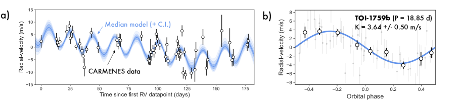
Figure 3: CARMENES radial-velocity follow-up of TOI-1759. a) Our CARMENES radial-velocity campaign (white points with black errorbars; first point corresponding to $2459054.56851$) had a total duration of about 6 months, over which we were able to detect both a radial-velocity variation at 18.85 d, along with a long-term signal here modeled as a GP. The blue line with transparent bands around it indicate our full (GP + planetary) median signal, along with its 68, 95 and 99% credibility intervals, respectively. b) Phase-folded radial-velocity curve at the period of the transiting exoplanet TOI-1759 b ($P=18.85$ d; grey points, binned datapoints covering about 2 d plotted as white points with black errorbars). The semi-amplitude we obtain for this signal is $3.64\pm 0.50$ m s^-1.

2.3 Ground-based photometry

Ground-based photometric follow-up observations were performed as part of the TESS Follow-up Program’s (TFOP) Subgroup 1 (SG1). Among the observations, a transit of TOI-1759 b in May 21, 2020, was captured by three independent telescopes/observatories: the OAA telescope in the Observatori Astronòmic Albanyà (Albanyà, Spain; 4 hours of total observing time, per point precision of 1140 ppm at 1-minute cadence; $R$-filter observations), the RCO telescope in the Grand-Pra observatory (Valais Sion, Switzerland; 6 hours of total observing time, per point precision of 1080 ppm at 1.3-minute cadence; $i_{p}$-filter observations), and the OMC telescope in the Montcabrer observatory (Barcelona, Spain; 5 hours of total observing time, per point precision of 1500 ppm at 1.9-minute cadence; $I_{c}$-filter observations). Data reduction for the OAA and OMC observations was performed in a two-step process: the MaximDL image processing software was used to perform image calibration (bias, darks, flats), while differential photometry was obtained using the AstroImageJ software (Collins et al., 2017). For the RCO observations, image calibration and differential photometry were both performed using AstroImageJ. The data, along with a best-fit model transit after subtracting the best-fit systematics model for each dataset (see Section 3 for details), is presented in Figure 4. The data are also presented in Table 6.

The observed transits by these three independent observatories on May 21, 2020 not only confirmed that the event observed by TESS was on-target (i.e., happened on TOI-1759), but in practice confirmed that the real period of the event was 18.85 d (i.e., half the period proposed by the TESS data validation reports), with the duration and depth detected by those observatories being consistent with the duration and depth observed in the TESS transit events.

Long-term photometric monitoring was also performed from the ground using the 0.8 m Joan Oró telescope (TJO; Colomé et al., 2010) at the Montsec Observatory in Lleida, Spain and the 90-cm telescope at the Sierra Nevada Observatory (SNO; Amado et al., 2021). For the TJO observations, the data were obtained from June 2020 to April 2021, spanning for more than 300 d and covering 107 different nights. We obtained a total of 1331 images with an exposure time of 40 seconds using the Johnson $R$ filter of the LAIA imager, a 4k×4k CCD with a field of view of 30^′ and a scale of 0.4^′′/pixel. The SNO data were obtained from April to August, 2021, spanning 135 d and collecting observations on 55 different nights. Each night, 20 exposures per filter were obtained using both Johnson $V$ and $R$ filters, with exposure times of 60 and 40 seconds, respectively. The photometry from these exposures was averaged to obtain a single photometric value per filter each night. These data were obtained with a VersArray 2k×2k CCD camera with a field of view of 13.2x13.2 arcmin² and a scale of 0.4 arcsec/pixel as well.

The TJO CCD images were calibrated with darks, bias and flat fields with the ICAT pipeline (Colome & Ribas, 2006). The differential photometry was extracted with AstroImageJ (Collins et al., 2017) using the aperture size that minimized the rms of the resulting relative fluxes, and a selection of the 30 brightest comparison stars in the field which did not show variability. Then, we used our own pipelines to remove outliers and measurements affected by poor observing conditions or presenting a low signal-to-noise ratio. This resulted in a total of 1087 measurements in the final data set with an rms of 6 ppt (parts per thousand).

In a similar way, the SNO resulting light curves were obtained by the method of synthetic aperture photometry. Each CCD frame was also corrected in a standard way for bias and flat-fielding. Different aperture sizes were tested in order to choose the best one for our observations. A number of nearby and relatively bright stars within the frames were selected as reference stars to produce differential photometry of TOI-1759. Finally, outliers due to poor observing conditions or very high airmass were removed. This resulted in a total of 1029 and 1027 individual data points in filters V and R, respectively, with rms of 6.1 and 6.4 ppt.

Both the TJO and SNO datasets are presented in Table 7. An analysis of these datasets is presented in Section 3.2.

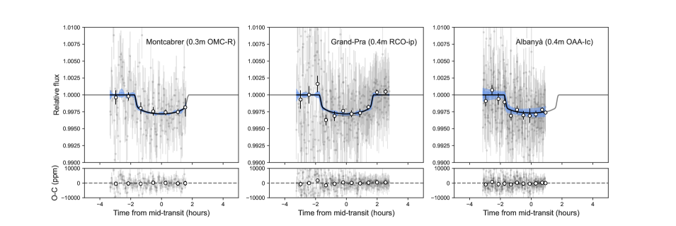
Figure 4: Ground-based follow-up transit photometry of TOI-1759 b. Transit of TOI-1759 b on May 21, 2020, captured by three different observatories: the OAA telescope in the Observatori Astronòmic Albanyà, the RCO telescope in the Grand-Pra Observatory and the OMC telescope in the Motcabrer Observatori. The duration and depth of the event is consistent between instruments.

2.4 High-resolution imaging

To help rule out stellar multiplicity and close blends with nearby stars and to obtain more precise planetary radii by accounting for close-in stellar blends (Ciardi et al., 2015; Schlieder et al., 2021), we observed TOI-1759 with both the ’Alopeke speckle imaging camera (Scott & Howell, 2018) on the 8 m Gemini North telescope and the NIRC2 near-infrared adaptive-optics fed camera on the 10 m Keck-II telescope. The optical and NIR high resolution imaging complement each other with higher resolution in the optical but deeper sensitivity (especially to low-mass stars) in the infrared.

’Alopeke obtains diffraction-limited imaging in two simultaneously-imaged narrow bands centered at 562 and 832 nm. Due to the relative faintness of the target star at these wavelengths, we obtained five exposures in each channel, with integration times of 60 ms each. We reduced the data using standard techniques using the methods described by Matson et al. (2019). The resulting contrast curves and reconstructed 832 nm image, all shown in Fig. 5. The optical speckle observations show no evidence of an additional stellar companion.

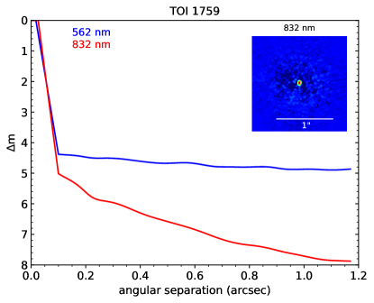
Figure 5: High spatial resolution imaging of TOI-1759. Two-band speckle imaging observations obtained with the Alopeke speckle imaging camera on the 8 m Gemini North telescope for TOI-1759 reveal no close-companion down to $0.1$”, dimmer than about $\Delta m=$ 4-5 mag than the target.

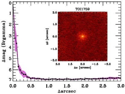
Figure 6: Near-infrared high spatial resolution imaging of TOI-1759. NIRC2 imaging observations obtained for TOI-1759 on Keck-II reveals no close-companion down to $0.1\,\arcsec$, dimmer than about $\Delta m=$ 4-5 mag than the target.

TOI-1759 was also observed with the NIRC2 instrument on Keck-II behind the natural guide star AO system (Wizinowich et al., 2000). The observations were made on 2020 Sep 09 UT in the standard 3-point dither pattern that is used with NIRC2 to avoid the left lower quadrant of the detector which is typically noisier than the other three quadrants. The dither pattern step size was $3\arcsec$ and was repeated twice, with each dither offset from the previous dither by $0.5\arcsec$. The camera was in the narrow-angle mode with a full field of view of $\sim 10\arcsec$ and a pixel scale of approximately $0.0099\arcsec$ per pixel. The observations were made in the narrow-band $Br$-$\gamma$ filter $(\lambda_{o}=2.1686;\Delta\lambda=0.0326\mu$m) with an integration time of 1 seconds with one coadd per frame for a total of 9 seconds on target.

The AO data were processed and analyzed with a custom set of IDL tools. The science frames were flat-fielded and sky-subtracted. The flat fields were generated from a median average of dark subtracted flats taken on-sky, and the flats were normalized such that the median value of the flats is unity. Sky frames were generated from the median average of the 9 dithered science frames; each science image was then sky-subtracted and flat-fielded. The reduced science frames were combined into a single combined image using a intra-pixel interpolation that conserves flux, shifts the individual dithered frames by the appropriate fractional pixels, and median-coadds the frames. The final resolution of the combined dithers was determined from the full-width half-maximum of the point spread function; 0.049″. The sensitivities of the final combined AO image were determined by injecting simulated sources azimuthally around the primary target every $20^{\circ}$ at separations of integer multiples of the central source’s FWHM (Furlan et al., 2017). The brightness of each injected source was scaled until standard aperture photometry detected it with $5\sigma$ significance. The resulting brightness of the injected sources relative to the target set the contrast limits at that injection location. The final $5\sigma$ limit at each separation was determined from the average of all of the determined limits at that separation and the uncertainty on the limit was set by the rms dispersion of the azimuthal slices at a given radial distance. The final combined image and sensitivity curve are shown in Fig. 6

Both the optical speckle and the near-infrared adaptive optics observations find no additional stars (down to 0.1” dimmer than about 4-5 magnitudes than the target in the optical and near-infrared) and so further strengthen the case for TOI-1759 b being a bona fide planet.

3 Analysis

3.1 Stellar parameters

We obtained the photospheric parameters $T_{\rm eff}$, $\log{g}$  and ${\rm[Fe/H]}$ of TOI-1759 following Passegger et al. (2019) by fitting PHOENIX synthetic spectra to the combined (co-added) CARMENES VIS spectrum described in Section 2.2.1, which has a signal-to-noise ratio in the VIS channel of $\approx$ 200. We used $v\sin{i}=2$ km s^-1, which was measured by Marfil et al. (2021) as an upper limit. We derived its luminosity following Cifuentes et al. (2020) by using the latest parallactic distance from Gaia EDR3 (Gaia Collaboration et al., 2021), and by integrating Gaia, 2MASS (Skrutskie et al., 2006) and AllWISE (Cutri et al., 2014) photometry covering the full spectral energy distribution with the Virtual Observatory Spectral energy distribution Analyser (Bayo et al., 2008). The stellar radius follows from Stefan-Boltzmann’s law and the stellar mass by using the linear mass-radius relation from Schweitzer et al. (2019).

TOI-1759’s pseudo equivalent width of the H$\alpha$ line as defined by Schöfer et al. (2019) is pEW${}^{\prime}({{\rm H}\alpha})<-0.3$ Å (Marfil et al., 2021), classifying it as an H$\alpha$ inactive star. Furthermore, Marfil et al. (2021) assign it to the Galactic thin disc population, which has a maximum age of about 8 Gyr (Fuhrmann, 1998). Using these two properties as age indicators, we conclude that its age is between 1 Gyr (the typical minimum age for field stars) and 8 Gyr without being able to be more precise. All collected and derived parameters are presented in Table 3.1.

Table 1: Stellar properties of TOI-1759.

Parameter	Value	Reference
Names	TIC 408636441	TIC
	2MASS J1472477+6245139	2MASS
	TYC 4266-00736-1	Tycho-2
	WISEA J214724.51+624513.8	AllWISE
RA (J2000)	21h47m24$\fs$39	Gaia EDR3
DEC (J2000)	62°45′13$\farcs$7	Gaia EDR3
Spectral type	M0.0 V	Lep13
$\mu_{\alpha}\cos{\delta}$ [mas yr-1]	–173.425 $\pm$ 0.012	Gaia EDR3
$\mu_{\delta}$ [mas yr-1]	–10.654 $\pm$ 0.011	Gaia EDR3
$\pi$ [mas]	24.922 $\pm$ 0.010	Gaia EDR3
$d$ [pc]	40.112 $\pm$ 0.016	Gaia EDR3
$G_{BP}$ [mag]	11.7164 $\pm$ 0.0029	Gaia EDR3
$G$ [mag]	10.8386 $\pm$ 0.0028	Gaia EDR3
$T$ [mag]	9.9284 $\pm$ 0.0073	TIC
$G_{RP}$ [mag]	9.9174 $\pm$ 0.0038	Gaia EDR3
$J$ [mag]	8.771 $\pm$ 0.043	2MASS
$H$ [mag]	8.114 $\pm$ 0.059	2MASS
$K_{s}$ [mag]	7.930 $\pm$ 0.020	2MASS
$W1$ [mag]	7.825 $\pm$ 0.027	AllWISE
$W2$ [mag]	7.886 $\pm$ 0.020	AllWISE
$W3$ [mag]	7.787 $\pm$ 0.018	AllWISE
$W4$ [mag]	7.643 $\pm$ 0.111	AllWISE
$L_{\star}$ [10-4 ${\rm L}_{\odot}$]	876.7 $\pm$ 6.3	This work
$T_{\rm eff}$  [K]	4065 $\pm$ 51	This work
$\log{g}$  [dex]	4.65 $\pm$ 0.04	This work
${\rm[Fe/H]}$  [dex]	0.05 $\pm$ 0.16	This work
$v\sin{i}$ [km s-1]	$\leq$ 2	Mar21
$M_{\star}$  [${\rm M}_{\odot}$]	0.606 $\pm$ 0.020	This work
$R_{\star}$  [${\rm R}_{\odot}$]	0.597 $\pm$ 0.015	This work
Age [Gyr]	1–8	This work
$\rho_{\star}$  [kg m-3]	3949 $\pm$ 323	This work

References. — 2MASS (Skrutskie et al., 2006), AllWISE (Cutri et al., 2014), Gaia EDR3 (Gaia Collaboration et al., 2021), Lep13 (Lépine et al., 2013), Mar21 (Marfil et al., 2021), TIC (Stassun et al., 2019), Tycho-2 (Høg et al., 2000).

3.2 Radial-velocity analysis

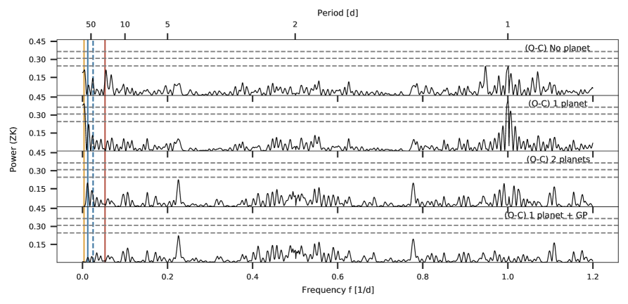
Figure 7: Generalized Lomb-Scargle (GLS) periodograms of the CARMENES radial-velocity data after subtracting different models. The power at each frequency corresponds to the one defined in Zechmeister & Kürster (2009, ZK in the labels above). The period of the transiting planet, $P=18.85$ d, is marked by the red solid line and the stellar rotation period, $P\approx 80$ d, and its first harmonic with the blue solid and dashed lines respectively. Further, the additional present long term periodicity with $P\approx 270$ d is marked by the yellow solid line. The horizontal dashed grey lines show the analytical false alarm probabilities (FAP) of 10, 1, and 0.1%. The top panel corresponds to the mean-substracted CARMENES radial-velocity dataset.

We performed a detailed analysis on the radial-velocities described in Section 2.2.1 in order to constrain the possible signals arising from these data. To this end, we performed a suite of model fits to the radial-velocity data using juliet (Espinoza et al., 2019), in order to measure the evidence for a planet in the data using Bayesian evidences, $Z=P(\textnormal{Model}|\textnormal{Data})$. The fits were performed using the Dynamic Nested Sampling algorithm implemented in the dynesty library (Speagle, 2020).

We considered three main types of radial velocity models. The first was a “no planet” model, namely, a set of models in which it is assumed there is no planetary signal present in the radial-velocity data, and which thus assumes the data are either consistent with a flat line or with correlated noise modeled through a Gaussian process (GP). The second class were “1-planet” models; these considered the presence of a planetary signal in the radial-velocity data (modeled as a circular orbit), and a suite of possible extra signals, such as linear or quadratic trends, or a (quasi-periodic) GP. Finally, we also considered the possibility that the data was best explained by a “2-planet” model, as a sum of two circular orbits and a suite of possible extra signals, such as a linear, quadratic or a GP trend.

We first performed “blind” fits to the data — that is, fits in which we assumed no strong prior knowledge on the signal(s) present on our radial-velocities. For our GP, we assumed a quasi-periodic kernel of the form

$$k(t_{i},t_{j})=\sigma^{2}_{GP}\exp\left(-\alpha\tau^{2}-\Gamma\sin^{2}\left[\frac{\pi\tau}{P_{rot}}\right]\right),$$

where $\tau=|t_{i}-t_{j}|$. We set log-uniform priors for $\sigma_{GP}$, $\alpha$ and $\Gamma$, with lower and upper limits of $(0.01,100)$ m s^-1, $(10^{-10},1)$ d^-1 and $(0.01,100)$ respectively, based on the experiments performed with this kernel in Stock et al. (2020a) and Stock et al. (2020b), and a uniform prior for $P_{rot}$ between 0.5 (half the best sampling in our radial-velocities) and 350 d (two-times our time-baseline). The linear and quadratic trends both had uniform priors on the coefficients of $(10^{-3},10^{3})$. As for the circular orbits, we set a uniform prior on the period of the first one from $0.5$ to 50 d (so as to cover the 18 and 36-day periods which could possibly originate from the transiting exoplanet), and a uniform prior on the period of the second one from 50 to 350 d. Uniform priors were set for the time of inferior conjunction for both covering the entire time-baseline of our observations, the semi-amplitude — between 0 and 100 m s^-1 — and the systematic radial velocity — between -100 and 100 m s^-1. A jitter term, $\sigma_{w}$ was added to all our fits with a log-uniform prior between 0.01 and 100  m s^-1.

In our “blind” fits, we found that all models considering a periodic component were consistent with a prominent signal at $\sim 18.5$ d, which corresponds to the transit signal implied by the TESS photometry presented in Section 2.1 and the ground-based transits presented in Section 2.3. The model with the highest evidence in our set of fits was one composed of a sinusoid plus a quasi-periodic GP ($|\Delta\log Z|\approx 4.3$, compared with the no-planets model). Given the high-resolution imaging data presented in Section 2.4, the ground-based transit detected on-target presented in 2.3 and the fact that the period of the planetary signal for the model with the highest evidence ($18.49^{+0.23}_{-0.21}$ d) agrees with the period implied by the photometric data ($18.8480\pm 0.0010$ d), we consider that this 18-day period signal in both photometry and radial-velocities is, indeed, a bona fide transiting exoplanet.

Having concluded that the 18-day period signal is indeed a bona fide transiting exoplanet, we then focused on finding the best model that explains the radial-velocity dataset. We considered the same class of models and priors as the ones presented above, but now for the first planet we fixed the period and transit center to the values defined by a photometric fit made to the data using juliet (see Section 3.3 for details on the priors of that fit): period $P=18.85008\pm 0.00018$ d, and time-of-transit center $t_{0}=2458745.4651\pm 0.0015$ d. A compilation of the log-evidences for each of the fits we performed is presented in Table 2. As can be seen, the model with the highest evidence is once again a 1-planet + GP model. Interestingly, however, this model is in practice indistinguishable ($|\Delta\log Z|<2$; Trotta, 2008) from most of the 2-planet models (except the 2-planet + linear trend model). It is also indistinguishable from all those models considering either one or both of them having eccentric orbits.

Table 2: Log-evidence differences $\Delta Z$ between different models considered for our radial-velocity-only analysis, assuming one of the Keplerian signals to have the same ephemerides as those implied by the observed transits. Below, a flat-line model includes only a systematic radial-velocity and a jitter term. The GP refers to a Gaussian Process with a quasi-periodic kernel. See text for details on the priors.

Model	$\ln\Delta Z$
No planet models
Flat line	–9.4
GP	–6.6
1 planet models
1 planet + linear trend	–23.6
1 planet + quadratic trend	–9.1
1 planet	–8.8
1 planet + GP	0
2 planet models
2 planet + linear trend	–12.6
2 planet	–1.6
2 planet + GP	–1.4
2 planet + quadratic trend	–1.3

It is interesting to note that the posterior distribution function of the GP rotation period of the 1-planet + GP model, $P_{\textrm{rot}}$, shows a bimodal distribution, with peaks at $\sim 80$ d and $>150$ d. In the 2-planet + GP model, the latter long periodic signal is picked up by the second sinusoid and is constrained to be about $270\pm 60$ d, while the quasi-periodic component of the GP shows again an accumulation of samples with higher likelihood at $\sim 80$ d. A Generalized Lomb-Scargle (GLS, Zechmeister & Kürster, 2009) periodogram analysis of the residuals of each of those models is presented in Figure 7, in order to further explore the nature of these long-period signals. If the signal of the transiting planet is subtracted (second panel), a significant power excess is apparent at $\sim 270$ d (which is above the baseline of our observations, which was 175 d) and next to it, even though insignificant, a peak at $\sim 80$ d. The latter is independent of the long term variation, as it is still present after fitting the transiting planet together with the $\sim 270$ d signal (third panel).

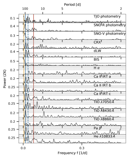
Figure 8: GLS periodograms of the TJO photometry, SNO photometry and the CARMENES spectral activity indicators. Analogous to the periodograms of the RVs, the period of the transiting planet, $P=18.85$ d and the additional present long term periodicity with $P\approx 270$ d are marked by the solid red and yellow lines, respectively. The stellar rotation period, $P\approx 80$ d, and its first harmonic are indicated by the blue solid and dashed lines. The horizontal dashed grey lines show the analytical false alarm probabilities (FAP) of 10, 1, and 0.1%.

To find out whether the $\sim 80$ d signal or the $\sim 270$ d power excess could be attributed to stellar activity, we investigated the activity indicators that are routinely derived from the CARMENES spectra (see Zechmeister et al., 2018; Schöfer et al., 2019; Lafarga et al., 2020, for the full list of indicators and how they are calculated). In Figure 8 we show the GLS periodograms of several activity indicators and the long term photometry presented in Section 2.3. Almost all indicators, as well as the photometry, show consistent signals around 80 and/or 40 d, which would explain the $\sim 80$ d seen in the RVs as the stellar rotation period. If indeed the rotation period of the star is 80 days, the 40-day signal could be interpreted as spots at opposite longitudes and/or a by-product of the not-strictly-periodic nature of the signal. Further, the TJO data, the BIS and the Ca ii IRT b and c also show a long term trend, which might be related with the $\sim 270$ d power excess.

Given that we could not rule out a stellar origin for the $\sim 80$ d signal and the $\sim 270$ d power excess, and that the 1-planet + GP model has the highest evidence for our RV data and can account for all significant signals in the data (see the residuals in the last panel of Figure 7), we consider this model for the global modelling of the data which we present in the next subsection. We note that we also tested fitting our global model using the rest of the models in Table 2 which are indistinguishable to the one being selected here, and all of them gave rise to similar constraints in the final parameters of the transiting exoplanet.

3.3 Global modeling

We performed a global modelling of the radial-velocity and photometric data using the juliet library (Espinoza et al., 2019) in order to jointly constrain the planetary properties from the photometry and radial-velocity datasets outlined in previous sections. As in the radial-velocity analysis presented in 3.2, we once again use the Dynamic Nested Sampling algorithm implemented in the dynesty library (Speagle, 2020).

For the TESS photometry, we decided to use a GP to consider residual systematic trends in the PDC lightcurves under use in this work. We used an Exponential-Matérn kernel (i.e., the product of an exponential and a Matérn 3/2 kernel) as implemented in the celerite library (Foreman-Mackey et al., 2017) via juliet, with hyperparameters (GP amplitude, $\sigma_{GP}$, and two time-scales: one for the Matèrn 3/2 part of the kernel, $\rho$, and another for the exponential part of the kernel, $T$) which are individual to each of the sectors; a jitter term is also added in quadrature to the covariance matrix for each sector. A quadratic law is used to constrain limb-darkening, where the coefficients are shared between the different sectors; we use the parametrization of Kipping (2013) instead of fitting for the limb-darkening coefficients directly. For the ground-based photometry, we found that airmass was a very good predictor of the long-term trends in the data, and so we added this as a linear regressor in our fit — weighted by a coefficient $\theta$, which is different for each instrument and is jointly fit with the rest of the parameters of the global fit. In addition, we observed that this linear regressor was insufficient to model all the correlated noise leftover on the OMC and RCO datasets. We thus decided to fit those with an additional Matèrn 3/2 kernel. A linear limb-darkening law was used for all ground-based instruments, as a higher order law was not necessary given the lower photometric precision (see, e.g. Espinoza & Jordán, 2016). An individual jitter term was added to the diagonal of the covariance matrix on each of to those datasets as well. For the radial-velocities, following our results in Section 3.2, we consider a 1-planet model plus a quasi-periodic GP as the model to be fit in our joint analysis. We set a wide prior for the systemic radial-velocity, as well as for the jitter term and the hyperparameters of the GP — in particular, for the period of the quasi-periodic GP $P_{\textrm{rot}}$, we use a wide period between 20 and 350 d in order to cover the two possible periods for this parameter observed in Section 3.2. The full definition of the priors and corresponding posteriors of our joint fit are given in Table 3.

Table 3: Prior and posterior parameters of the global fit performed to TOI-1759. For the priors, $N(\mu,\sigma^{2})$ stands for a normal distribution with mean $\mu$ and variance $\sigma^{2}$, $TN(\mu,\sigma^{2};a,b)$ is a truncated normal distribution with lower and upper limits given by $a$ and $b$, respectively; $U(a,b)$ and $\log U(a,b)$ stands for a uniform and log-uniform distribution between $a$ and $b$, respectively.

Parameter	Prior	Posterior
Stellar & planetary parameters
$P_{1}$ [d]	$N(18.85,0.1^{2})$	$18.85019\pm 0.00013$
$t_{0,1}$ (BJD)	$N(2458745.45,0.1^{2})$	$2458745.4654\pm 0.0011$
$R_{p,1}/R_{\star}$	$U(0.0,1.0)$	$0.0483\pm 0.0010$
$b_{1}=(a/R_{\star})\cos(i)$	$U(0.0,1.0)$	$0.21^{+0.09}_{-0.10}$
$K_{1}$ [m s-1]	$U(0,100)$	$3.64^{+0.50}_{-0.51}$
$e_{1}$	fixed	0
$\omega_{1}$	fixed	90
$\rho_{\star}$ [kg m-3]	$TN(3949,323^{2};1000,10000)$	$3970^{+218}_{-233}$
TESS photometry instrumental parameters
$q_{1,TESS}^{a}$	$U(0,1)$	$0.32^{+0.24}_{-0.14}$
$q_{2,TESS}^{a}$	$U(0,1)$	$0.46^{+0.28}_{-0.25}$
$m_{\textnormal{flux,16}}$ [ppm]	$U(0,10^{5})$	$851^{+7916}_{-7770}$
$m_{\textnormal{flux,17}}$ [ppm]	$U(0,10^{5})$	$-1598^{+8062}_{-8089}$
$m_{\textnormal{flux,24}}$ [ppm]	$U(0,10^{5})$	$428^{+7904}_{-7797}$
$\sigma_{\textnormal{w,16}}$ [ppm]	$\log U(0.1,10^{5})$	$1.8^{+7.5}_{-1.5}$
$\sigma_{\textnormal{w,17}}$ [ppm]	$\log U(0.1,10^{5})$	$2.9^{+15.1}_{-2.5}$
$\sigma_{\textnormal{w,24}}$ [ppm]	$\log U(0.1,10^{5})$	$1.9^{+7.7}_{-1.6}$
$\sigma_{\textnormal{GP,16}}$ [ppm]	$\log U(10^{-4},10^{2})$	$0.000104^{+0.000047}_{-0.0000026}$
$\sigma_{\textnormal{GP,17}}$ [ppm]	$\log U(10^{-4},10^{2})$	$0.000106^{+0.000067}_{-0.0000040}$
$\sigma_{\textnormal{GP,24}}$ [ppm]	$\log U(10^{-4},10^{2})$	$0.000100^{+0.000030}_{-0.0000017}$
$\rho_{\textnormal{GP,16}}$ [d]	$\log U(10^{-3},10^{2})$	$73^{+16}_{-17}$
$\rho_{\textnormal{GP,17}}$ [d]	$\log U(10^{-3},10^{2})$	$74^{+15}_{-18}$
$\rho_{\textnormal{GP,24}}$ [d]	$\log U(10^{-3},10^{2})$	$76^{+14}_{-17}$
$T_{\textnormal{GP,16}}$ [d]	$\log U(10^{-3},10^{2})$	$0.0010^{+0.000047}_{-0.000026}$
$T_{\textnormal{GP,17}}$ [d]	$\log U(10^{-3},10^{2})$	$0.0011^{+0.000081}_{-0.000045}$
$T_{\textnormal{GP,24}}$ [d]	$\log U(10^{-3},10^{2})$	$0.0010^{+0.000034}_{-0.000019}$
Ground-based photometry instrumental parameters
$q_{1,OAA}$	$U(0,1)$	$0.41^{+0.27}_{-0.24}$
$q_{1,OMC}$	$U(0,1)$	$0.55^{+0.27}_{-0.31}$
$q_{1,RCO}$	$U(0,1)$	$0.50^{+0.30}_{-0.29}$
$m_{\textnormal{flux,OAA}}$ [ppm]	$U(0,10^{5})$	$-2148^{+214}_{-216}$
$m_{\textnormal{flux,OMC}}$ [ppm]	$U(0,10^{5})$	$7936^{+6471}_{-6203}$
$m_{\textnormal{flux,RCO}}$ [ppm]	$U(0,10^{5})$	$-979^{+6296}_{-5945}$
$\sigma_{\textnormal{w,OAA}}$ [ppm]	$\log U(0.1,10^{5})$	$3395^{+146}_{-140}$
$\sigma_{\textnormal{w,OMC}}$ [ppm]	$\log U(0.1,10^{5})$	$3123^{+202}_{-190}$
$\sigma_{\textnormal{w,RCO}}$ [ppm]	$\log U(0.1,10^{5})$	$4143^{+165}_{-158}$
$\theta_{\textnormal{OAA}}$ [d]	$U(-10,10)$	$0.00112^{+0.00022}_{-0.00021}$
$\theta_{\textnormal{OMC}}$ [d]	$U(-10,10)$	$-0.0036^{+0.015}_{-0.015}$
$\theta_{\textnormal{RCO}}$ [d]	$U(-10,10)$	$0.013^{+0.015}_{-0.015}$
$\sigma_{\textnormal{GP,OMC}}$ [ppm]	$\log U(10^{-4},10^{2})$	$0.117^{0.022}_{-0.012}$
$\rho_{\textnormal{GP,OMC}}$ [d]	$\log U(10^{-3},10^{2})$	$0.438^{+0.040}_{-0.059}$
$\sigma_{\textnormal{GP,RCO}}$ [ppm]	$\log U(10^{-4},10^{2})$	$0.117^{0.019}_{-0.011}$
$\rho_{\textnormal{GP,RCO}}$ [d]	$\log U(10^{-3},10^{2})$	$0.438^{+0.039}_{-0.051}$
Radial-velocity instrumental/activity parameters
$\mu_{\rm CARMENES}$ [m s-1]	$U(-100,100)$	$0.1^{+4.7}_{-4.0}$
$\sigma_{w,\rm CARMENES}$ [m s-1]	$\log U(0.01,100)$	$1.85^{+0.50}_{-0.49}$
$\sigma_{\textnormal{GP,\rm CARMENES}}$ [m s-1]	$\log U(0.01,10^{2})$	$5.8^{+7.3}_{-2.5}$
$\alpha_{\textnormal{GP,\rm CARMENES}}$ (d-1)	$\log U(10^{-10},1)$	$0.000011^{+0.000433}_{-0.000011}$
$\Gamma_{\textnormal{GP,\rm CARMENES}}$	$\log U(0.01,100)$	$0.5^{+2.8}_{-0.5}$
$P_{\textnormal{GP,\rm Rot}}$	$U(20,350)$	$237^{+67}_{-103}$

Table 4: Derived properties for TOI-1759 b.

Parameter	Posterior	Description
$R_{p}$ [$R_{\oplus}$]	$3.14\pm 0.10$	Planetary radius
$M_{p}$ [$M_{\oplus}$]	$10.8\pm 1.5$	Planetary mass
$i$ [deg]	$89.72\pm 0.13$	Orbital inclination
$T_{14}$ [hours]	$3.23\pm 0.13$	Transit duration
$a$ [au]	$0.1177\pm 0.0038$	Semi-major axis of the orbit
$T_{eq,0}$ [K]	$443\pm 7$	Equilibrium temperaturea
		(assuming 0 albedo)
$T_{eq,0.3}$ [K]	$405\pm 6$	Equilibrium temperaturea
		(assuming 0.3 albedo)
$S_{p}$ [$S_{\oplus}$]	$6.39\pm 0.41$	Stellar irradiation
		on the planet
$\rho_{p}$ [g cm-3]	$1.91\pm 0.32$	Planetary bulk density
$g_{p}$ [m s-2]	$10.7\pm 1.6$	Planetary surface gravity

The resulting best-fit models and corresponding credibility bands are presented in Figure 2 for the TESS photometry, in Figure 4 for the ground-based photometry and in Figure 3 for the radial-velocities. The constraints from our radial-velocity follow-up allowed us to obtain a precise ($>5\sigma$ above 0) measurement of the semi-amplitude imprinted by TOI-1759 b on its star of $K=3.64^{+0.50}_{-0.51}$ m s^-1, which is an over 7-sigma detection of the semi-amplitude. Joining the derived transit and radial-velocity parameters, along with the stellar properties presented in Table 3.1, we derive the fundamental parameters of TOI-1759 b in Table 4. As can be observed, TOI-1759 b is a relatively cool (443 K equilibrium temperature assuming 0 albedo) sub-Neptune-sized exoplanet ($R_{p}=3.14\pm 0.10\,R_{\oplus}$). Coupling these numbers with our estimated mass of $M_{p}=10.8\pm 1.5M_{\oplus}$, we derive a planetary bulk density ($\rho_{p}=1.91\pm 0.32$ g cm^-3) and gravity ($g_{p}=10.7\pm 1.6$  m s^-2) which are strikingly similar to those of Neptune (1.64 g cm^-3 and 11.15 m s^-2, respectively). We discuss the properties of TOI-1759 b in context of other discovered systems in the next section.

4 Discussion

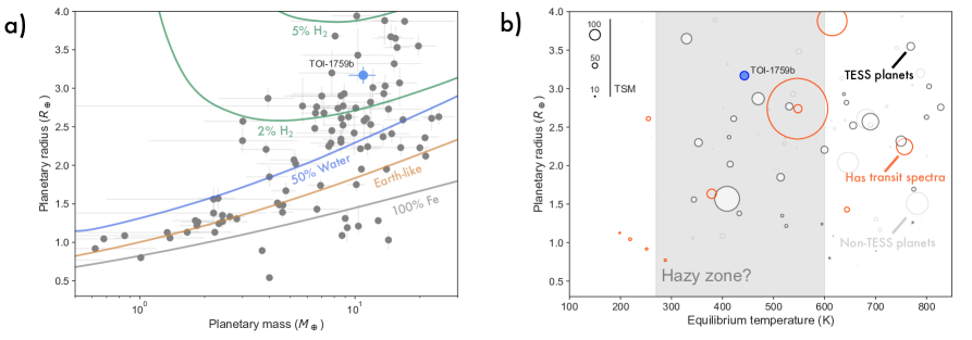
Figure 9: Properties of TOI-1759 b as compared to previously small, known exoplanets with measured mass and radius. a) Mass-radius diagram of all known small ($R_{p}<4\,R_{\oplus}$) exoplanets with $T_{\textnormal{eq}}<1000$ K (grey) and TOI-1759 b (blue). The mass-radius models are from Zeng et al. (2016) and show 100% Fe (grey), an Earth-like composition (32.5% Fe, 67.5% MgSiO₃ by mass, brown), a 50% Earth-like and 50% water-by-mass composition (blue) and Earth-like composition models with 2% and 5% H₂ on top of it (green). Water-rich models with 2% and 5% H₂ on top (i.e., Neptune-like compositions) are not shown, but would be indistinguishable with the green models in this panel given the size of the errorbars. b) Equilibrium temperature (assuming zero albedo) versus radius diagram for the same cuts made for panel a), showing the location of TESS planets (white markers), non-TESS planets (white transparent markers), planets that have previously been characterized via transmission spectroscopy with HST/WFC3 (red markers) and TOI-1759 b (blue). The size of the markers represents the value of the transmission spectroscopy metric (TSM Kempton et al., 2018); grey band shows the proposed region of hazy exoplanets by (Yu et al., 2021, see text for discussion).

In order to put TOI-1759 b in context with the known sample of small exoplanets, we query the properties of all such exoplanets that (a) have both a measured mass and radius, (b) are smaller than $R_{p}<4\,R_{\oplus}$ and (c) have equilibrium temperatures cooler than $1000$ K from the NASA Exoplanet Archive (NASA Exoplanet Science Institute, 2020) — i.e., a cut similar to that presented in Guo et al. (2020), but updated with the latest exoplanetary systems as of July 23, 2021. In Figure 9, we show the location of TOI-1759 b in both the planetary mass versus radius plane and the equilibrium temperature versus planetary radius plane.

In terms of its mass and radius, Figure 9a shows that TOI-1759 b is consistent with having a $2-5\%$ H₂ envelope, and an interior composition ranging from being an Earth-like one to being a scaled-down version of Neptune. Figure 9b, on the other hand, shows how TOI-1759 b adds up to the increasing number of small ($R_{p}<4\,R_{\oplus}$) worlds with measured mass and radius at relatively low equilibrium temperatures. In particular, TOI-1759 b falls on the very interesting region where the work of Yu et al. (2021) recently proposed exoplanet atmospheres to be hazy due to the lack of haze-removal processes at temperatures between about 300-600 K. It is interesting to note that TOI-1759 b falls exactly at the equilibrium temperature where Yu et al. (2021) predict the haziest exoplanets should be ($T_{eq,0.3}\sim 400$ K, where $T_{eq,0.3}$ means an equilibrium temperature calculated assuming an albedo of 0.3; see Table 4). The proposed trend presented in that work seems to be in line with observed transmission spectra for planets hotter than about 500 K (Crossfield & Kreidberg, 2017). For example, GJ 1214 b (550 K, Kreidberg et al., 2014, biggest red circle in Figure 9a) shows a significantly muted water feature, whereas HAT-P-11 b (750 K, Fraine et al., 2014, not shown in Figure 9a as $R_{p}=4.3\,R_{\oplus}$ for this exoplanet) has a $3-$scale height water amplitude in its transmission spectrum. However, the hypothesis is harder to test for temperate exoplanets ($<500$ K), as good targets for atmospheric characterization have remained scarce, in particular for small ($R_{p}<4\,R_{\oplus}$) planets.

TOI-1759 b is among the best temperate targets to perform transmission spectroscopy based on its Transmission Spectroscopy Metric (TSM Kempton et al., 2018). Following the work of Kempton et al. (2018), we estimate a TSM of $81\pm 14$, which puts it among the top five targets for atmospheric characterization to date at equilibrium temperatures lower than 500 K, together with L 98-59 d (TSM of 233; Cloutier et al., 2019; Kostov et al., 2019; Pidhorodetska et al., 2021), TOI-178 g (TSM of 114; Leleu et al., 2021), TOI-1231 b (TSM of 97; Burt et al., 2021) and LHS 1140 b (TSM of 89; Dittmann et al., 2017; Ment et al., 2019) — the latter having actually been recently characterized by HST/WFC3 (Edwards et al., 2021), reporting weak evidence for water absorption in its planetary atmosphere.

For a quantitative assessment of TOI-1759 b’s atmospheric characterization with JWST, we investigated a suite of atmospheric scenarios and calculated their JWST synthetic spectra using the photo-chemical model ChemKM (Molaverdikhani et al., 2019, 2020a), the radiative transfer model petitRADTRANS (Mollière et al., 2019, 2020), and ExoTETHyS (Morello et al., 2021) for uncertainty estimations.

Assuming an isothermal atmosphere with a temperature of 400 K and a constant vertical mixing of $K_{zz}$=$10^{6}$  cm² s^-1 results in persisting water and methane features in the transmission spectra of TOI-1759 b, see Figure 10. But such atmospheric features are expected to be suppressed in a high-metallicity atmosphere, see bottom panel in Figure 10. Considering haze in the atmosphere of TOI-1759 b further mutes the features and hence a hazy, high-metallicity atmosphere is expected to show a nearly flat transmission spectrum, see the blue line in Figure 10 bottom panel.

The PandExo package (Batalha et al., 2017) was used to determine the best configurations to observe with the NIRISS SOSS (0.6-2.8 $\mu$m), NIRSpec G395M (2.88-5.20 $\mu$m) and MIRI LRS (5-12 $\mu$m) instrumental modes. Then we used ExoTETHyS to compute the simulated spectra. The wavelength bins were specifically determined to have similar counts, leading to nearly uniform error bars per spectral point. Note that the minimal error bars output by ExoTETHyS have been multiplied by the reciprocal of the square root of the observing efficiency and a conservative factor 1.2 that accounts for correlated noise. The resulting error bars are equal to or slightly larger than those obtained with PandExo for the same wavelength bins. In particular, the spectral error bars estimated for just one transit observation per instrument configuration are 25-30 ppm at wavelengths $<$5 $\mu$m, and 45-50 ppm at wavelengths $>$5 $\mu$m, with several points to sample each molecular feature as shown in Figure 10). Comparing these uncertainties with the expected water and methane features of $\sim$200 ppm significance suggests the possibility of differentiating these scenarios during one transit only.

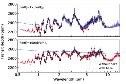
Figure 10: Synthetic JWST transmission atmospheric spectra of TOI-1759 b. Top : Fiducial models with solar abundance, Bottom : Enhanced metallicity by a factor of 100, by considering haze opacity (solid blue lines) and without haze opacity (solid red lines). Estimated uncertainties are shown for the observation of one transit with JWST NIRISS-SOSS, NIRSpec-G395M, and MIRI-LRS configurations.

TOI-1759 b, along with TOI-178 g ($R_{p}=2.87\,R_{\oplus}$, $T_{eq,0}=470$ K), TOI-1231 b ($R_{p}=3.65\,R_{\oplus}$, $T_{eq,0}=330$ K) and the (now) iconic K2-18 b ($R_{p}=2.61\,R_{\oplus}$, $T_{eq,0}=255$ K, Benneke et al., 2019; Tsiaras et al., 2019) form an excellent sample of sub-Neptunes to perform atmospheric characterization via transmission spectroscopy at equilibrium temperatures below 500 K. A sample that can be used to put the prediction of both proposed haze removal (Yu et al., 2021) and methane removal (Molaverdikhani et al., 2020b) processes to the test.

5 Conclusions

We have presented the discovery and characterization of the transiting exoplanet TOI-1759 b, a sub-Neptune ($R_{p}=3.14\pm 0.10\,R_{\oplus}$, $M_{p}=10.8\pm 1.5\,M_{\oplus}$) exoplanet on a 18.85-day orbit around an M dwarf star. The initial identification of the target was made thanks to precise TESS photometry, which unveiled three transits of the exoplanet in three different sectors with an ambigous period being consistent with both, a 18.85 and a 37.7-day period exoplanet. Thanks to ground-based photometric follow-up from different observatories, high-resolution spatial imaging and precise radial-velocities from the CARMENES high-resolution spectrograph, we were able to not only confirm TOI-1759 b as a bona fide transiting exoplanet and precisely measure its mass, but also constrain its true period to be $18.85019\pm 0.00013$ d.

TOI-1759 b adds to the growing number of temperate ($T_{\textnormal{eq}}<500$ K) exoplanets, and is a particularly promising target to perform atmospheric characterization on. Its equilibrium temperature ($T_{\textnormal{eq,0.3}}=405\pm 6$ K) puts it exactly where the work of Yu et al. (2021) predicts the haziest exoplanets to be, and thus provides an exciting system in which to test this proposal. In addition, our 6-month radial-velocity campaign revealed an 80-day periodicity in the data most likely arising from stellar activity, and a possible longer-term periodicity with a period $>200$ d. The current baseline of our CARMENES observations is insufficient to unveil the true nature of this latter long-period signal. However, a campaign spanning a longer baseline is needed in order to reveal the exact source and periodicity of this signal.

Appendix A Radial-velocity data

Our full CARMENES dataset for the VIS channel is presented in Table 5, along with the corresponding activity indicators at each epoch.

Table 5: Radial velocity measurements for the star along with activity indicators at each epoch.

Name	BJD	RV	$\sigma_{\rm RV}$	CRX	dLW	BIS	$\rm{H}_{\alpha}$	Ca II IRT a	Instrument	S/N
	-2450000	(m s-1)	(m s-1)	(m s-1 Np-1)	($10^{3}$ m2 s-2)	(km s-1)	(km s-1)	(km s-1)
TOI-1759	9054.56851	2.33	2.51	49.44	1.48	-0.0774	0.074	0.0094	CARMENES-VIS	119.4
TOI-1759	9067.60481	3.32	2.32	43.58	-0.04	-0.0646	0.082	0.0128	CARMENES-VIS	97.6
TOI-1759	9068.57556	1.86	1.86	29.70	-11.16	-0.0776	0.074	0.0290	CARMENES-VIS	94.3
TOI-1759	9069.59957	0.86	1.78	21.57	-5.31	-0.0635	0.054	0.0154	CARMENES-VIS	101.8
TOI-1759	9070.55690	2.17	1.85	7.88	-5.34	-0.0764	0.076	0.0237	CARMENES-VIS	111.2
TOI-1759	9076.57116	6.20	2.55	15.86	-22.86	-0.0763	0.078	0.0304	CARMENES-VIS	80.6
TOI-1759	9078.60935	8.44	2.01	18.62	-11.90	-0.0719	0.068	0.0068	CARMENES-VIS	103.2
TOI-1759	9079.59579	3.59	2.33	36.88	-16.68	-0.0677	0.079	0.0154	CARMENES-VIS	104.2
TOI-1759	9081.58773	6.10	2.47	-16.45	-19.67	-0.0604	0.079	0.0099	CARMENES-VIS	81.8
TOI-1759	9084.55634	0.35	1.48	-10.41	2.25	-0.0560	0.093	0.0120	CARMENES-VIS	103.7
TOI-1759	9087.59796	1.37	2.12	6.67	-1.17	-0.0517	0.069	0.0071	CARMENES-VIS	104.8
TOI-1759	9089.53629	-1.43	1.95	-8.83	-5.14	-0.0600	0.071	0.0110	CARMENES-VIS	109.4
TOI-1759	9090.55842	-3.51	2.75	-8.03	-14.72	-0.0490	0.069	0.0033	CARMENES-VIS	76.3
TOI-1759	9091.54399	-8.08	3.58	-32.14	-6.07	-0.0609	0.049	0.0216	CARMENES-VIS	48.5
					$\cdot\cdot\cdot$
TOI-1759	9173.30701	-3.00	2.43	-12.31	12.00	-0.0291	0.052	0.0104	CARMENES-VIS	93.4
TOI-1759	9174.31626	-2.65	1.89	-11.97	15.74	-0.0118	0.065	-0.0023	CARMENES-VIS	90.7
TOI-1759	9175.35015	6.53	2.21	-32.46	7.19	-0.0132	0.102	0.0127	CARMENES-VIS	77.8
TOI-1759	9176.32926	-10.27	2.28	-14.38	20.12	-0.0227	0.064	0.0020	CARMENES-VIS	114.3
TOI-1759	9177.32923	-1.93	1.78	-35.19	13.28	-0.0312	0.066	0.0014	CARMENES-VIS	111.0
TOI-1759	9178.28239	-11.01	1.90	-15.77	7.78	-0.0338	0.086	0.0099	CARMENES-VIS	95.8
TOI-1759	9183.29700	-10.37	2.20	-31.60	-2.18	-0.0157	0.071	0.0123	CARMENES-VIS	97.3
TOI-1759	9186.33693	-9.05	4.74	-45.55	-22.24	-0.0773	0.037	0.0161	CARMENES-VIS	27.1
TOI-1759	9187.30129	-1.25	3.31	-45.82	-24.91	-0.0299	0.103	-0.0038	CARMENES-VIS	50.3
TOI-1759	9193.27483	4.02	3.18	0.08	-0.95	-0.0247	0.084	-0.0052	CARMENES-VIS	64.2
TOI-1759	9196.26135	-8.36	2.97	-9.94	7.30	-0.0186	0.032	-0.0079	CARMENES-VIS	72.1
TOI-1759	9197.34852	-4.98	3.64	-22.89	-3.08	-0.0198	0.085	0.0218	CARMENES-VIS	57.4
TOI-1759	9209.39053	6.56	6.36	7.17	-27.90	-0.0371	0.026	0.0052	CARMENES-VIS	25.7
TOI-1759	9216.25949	1.84	5.71	-48.81	3.21	-0.0156	0.125	0.0121	CARMENES-VIS	38.2
TOI-1759	9218.29595	-5.22	2.45	-15.32	-17.68	-0.0126	0.082	0.0091	CARMENES-VIS	61.6
TOI-1759	9219.28687	-4.05	3.34	-61.08	-22.66	-0.0350	0.055	0.0109	CARMENES-VIS	47.8
TOI-1759	9231.28008	1.00	2.57	-4.70	3.51	-0.0059	0.052	-0.0024	CARMENES-VIS	92.8
TOI-1759	9232.28137	2.54	2.77	-4.43	10.19	-0.0298	0.052	-0.0001	CARMENES-VIS	96.4

Note. — Signal-to-noise ratio (S/N) for CARMENES-VIS data corresponds to the S/N at order 36 (at about $840$ nm). A sample of the full radial-velocity dataset and activity indicators are shown here. The entirety of this table is available in a machine-readable form in the online journal.

Appendix B Photometric data

Our full photometric dataset targeting transits of TOI-1759 is presented in Table 6. The long-term photometry is presented in Table 7.

Table 6: Photometric transits of the planet.

Name	BJD	Relative flux	Error	Instrument	Standarized airmass
	-2450000
TOI-1759	8738.65456	1.000458	0.001213	TESS - Sector 16	—
TOI-1759	8738.65594	0.999531	0.001211	TESS - Sector 16	—
TOI-1759	8738.65733	1.000397	0.001213	TESS - Sector 16	—
TOI-1759	8738.65872	1.001858	0.001212	TESS - Sector 16	—
TOI-1759	8738.66011	0.999702	0.001212	TESS - Sector 16	—
TOI-1759	8738.66150	0.999855	0.001212	TESS - Sector 16	—
TOI-1759	8738.66289	0.999816	0.001210	TESS - Sector 16	—
TOI-1759	8738.66428	0.999837	0.001209	TESS - Sector 16	—
TOI-1759	8738.66567	0.998040	0.001210	TESS - Sector 16	—
TOI-1759	8738.66706	0.998851	0.001212	TESS - Sector 16	—
TOI-1759	8738.66844	0.999615	0.001213	TESS - Sector 16	—
		$\cdot\cdot\cdot$
TOI-1759	8990.54955	0.995134	0.001107	Albanya-0.4m (OAA-Ic)	-1.372
TOI-1759	8990.55022	1.000704	0.001110	Albanya-0.4m (OAA-Ic)	-1.380
TOI-1759	8990.55090	0.998573	0.001110	Albanya-0.4m (OAA-Ic)	-1.388
TOI-1759	8990.55159	0.997527	0.001110	Albanya-0.4m (OAA-Ic)	-1.396
TOI-1759	8990.55225	0.999177	0.001110	Albanya-0.4m (OAA-Ic)	-1.403
TOI-1759	8990.55293	1.001281	0.001110	Albanya-0.4m (OAA-Ic)	-1.411
TOI-1759	8990.55360	0.998378	0.001107	Albanya-0.4m (OAA-Ic)	-1.419
TOI-1759	8990.55428	0.998890	0.001113	Albanya-0.4m (OAA-Ic)	-1.426
TOI-1759	8990.55496	0.998735	0.001113	Albanya-0.4m (OAA-Ic)	-1.434
TOI-1759	8990.55563	0.997969	0.001113	Albanya-0.4m (OAA-Ic)	-1.442

Note. — The Standarized Airmass column corresponds to the airmass values substracted by their mean and divided by their standard deviation. A sample of the full photometric dataset is shown here. The entirety of this table is available in a machine-readable form in the online journal or the source file used to generate this compiled PDF version.

Table 7: Long-term photometric measurements of TOI-1759.

Name	BJD	Relative flux	Error	Instrument
	-2450000
TOI-1759	9010.61701	0.993732	0.000714	Joan-Oro-0.8m (TJO)
TOI-1759	9010.61758	0.993128	0.000714	Joan-Oro-0.8m (TJO)
TOI-1759	9010.61813	0.991751	0.000714	Joan-Oro-0.8m (TJO)
TOI-1759	9010.61868	0.992962	0.000714	Joan-Oro-0.8m (TJO)
TOI-1759	9010.61923	0.992559	0.000714	Joan-Oro-0.8m (TJO)
TOI-1759	9010.61978	0.990158	0.000714	Joan-Oro-0.8m (TJO)
TOI-1759	9010.62033	0.990918	0.000714	Joan-Oro-0.8m (TJO)
TOI-1759	9010.62089	0.991625	0.000714	Joan-Oro-0.8m (TJO)
TOI-1759	9010.62145	0.992897	0.000719	Joan-Oro-0.8m (TJO)
TOI-1759	9010.62200	0.991557	0.000719	Joan-Oro-0.8m (TJO)
TOI-1759	9010.62255	0.991023	0.000719	Joan-Oro-0.8m (TJO)
		$\cdot\cdot\cdot$
TOI-1759	9457.65199	1.003121	0.001813	Sierra-Nevada-0.9m (SNO-V)
TOI-1759	9457.65339	1.005637	0.001809	Sierra-Nevada-0.9m (SNO-V)
TOI-1759	9457.65479	1.003229	0.001785	Sierra-Nevada-0.9m (SNO-V)
TOI-1759	9457.65619	1.003976	0.001838	Sierra-Nevada-0.9m (SNO-V)
TOI-1759	9457.65759	1.003824	0.001882	Sierra-Nevada-0.9m (SNO-V)
TOI-1759	9457.65899	1.006960	0.001844	Sierra-Nevada-0.9m (SNO-V)
TOI-1759	9457.66039	1.001677	0.001862	Sierra-Nevada-0.9m (SNO-V)
TOI-1759	9457.66320	1.000984	0.001788	Sierra-Nevada-0.9m (SNO-V)
TOI-1759	9457.66460	1.005191	0.001829	Sierra-Nevada-0.9m (SNO-V)
TOI-1759	9457.66600	1.002202	0.001869	Sierra-Nevada-0.9m (SNO-V)

Note. — A sample of the full photometric dataset is shown here. The entirety of this table is available in a machine-readable form in the online journal or the source file used to generate this compiled PDF version.

References

- Aller et al. (2020) Aller, A., Lillo-Box, J., Jones, D., Miranda, L. F., & Barceló Forteza, S. 2020, A&A, 635, A128
- Amado et al. (2021) Amado, P. J., Bauer, F. F., Rodríguez López, C., et al. 2021, A&A, 650, A188
- Batalha et al. (2017) Batalha, N. E., Mandell, A., Pontoppidan, K., et al. 2017, PASP, 129, 064501
- Bayo et al. (2008) Bayo, A., Rodrigo, C., Barrado Y Navascués, D., et al. 2008, A&A, 492, 277
- Benneke et al. (2019) Benneke, B., Wong, I., Piaulet, C., et al. 2019, ApJ, 887, L14
- Borucki et al. (2010) Borucki, W. J., Koch, D., Basri, G., et al. 2010, Science, 327, 977
- Burt et al. (2021) Burt, J. A., Dragomir, D., Mollière, P., et al. 2021, arXiv e-prints, arXiv:2105.08077
- Caballero et al. (2016) Caballero, J. A., Guàrdia, J., López del Fresno, M., et al. 2016, in Society of Photo-Optical Instrumentation Engineers (SPIE) Conference Series, Vol. 9910, Observatory Operations: Strategies, Processes, and Systems VI, ed. A. B. Peck, R. L. Seaman, & C. R. Benn, 99100E
- Ciardi et al. (2015) Ciardi, D. R., Beichman, C. A., Horch, E. P., & Howell, S. B. 2015, ApJ, 805, 16
- Cifuentes et al. (2020) Cifuentes, C., Caballero, J. A., Cortés-Contreras, M., et al. 2020, A&A, 642, A115
- Cloutier et al. (2019) Cloutier, R., Astudillo-Defru, N., Bonfils, X., et al. 2019, A&A, 629, A111
- Collins et al. (2017) Collins, K. A., Kielkopf, J. F., Stassun, K. G., & Hessman, F. V. 2017, AJ, 153, 77
- Colomé et al. (2010) Colomé, J., Francisco, X., Ribas, I., Casteels, K., & Martín, J. 2010, in Society of Photo-Optical Instrumentation Engineers (SPIE) Conference Series, Vol. 7740, Software and Cyberinfrastructure for Astronomy, ed. N. M. Radziwill & A. Bridger, 774009
- Colome & Ribas (2006) Colome, J., & Ribas, I. 2006, IAU Special Session, 6, 11
- Crossfield & Kreidberg (2017) Crossfield, I. J. M., & Kreidberg, L. 2017, AJ, 154, 261
- Cutri et al. (2014) Cutri et al., R. M. 2014, VizieR Online Data Catalog, 2328
- Dittmann et al. (2017) Dittmann, J. A., Irwin, J. M., Charbonneau, D., et al. 2017, Nature, 544, 333
- Dorn et al. (2017) Dorn, C., Venturini, J., Khan, A., et al. 2017, A&A, 597, A37
- Edwards et al. (2021) Edwards, B., Changeat, Q., Mori, M., et al. 2021, AJ, 161, 44
- Espinoza & Jordán (2016) Espinoza, N., & Jordán, A. 2016, MNRAS, 457, 3573
- Espinoza et al. (2019) Espinoza, N., Kossakowski, D., & Brahm, R. 2019, MNRAS, 490, 2262
- Foreman-Mackey et al. (2017) Foreman-Mackey, D., Agol, E., Angus, R., & Ambikasaran, S. 2017, AJ, 154, 220. https://arxiv.org/abs/1703.09710
- Fraine et al. (2014) Fraine, J., Deming, D., Benneke, B., et al. 2014, Nature, 513, 526
- Fuhrmann (1998) Fuhrmann, K. 1998, A&A, 338, 161
- Fulton & Petigura (2018) Fulton, B. J., & Petigura, E. A. 2018, AJ, 156, 264
- Fulton et al. (2018) Fulton, B. J., Petigura, E. A., Blunt, S., & Sinukoff, E. 2018, PASP, 130, 044504
- Furlan et al. (2017) Furlan, E., Ciardi, D. R., Everett, M. E., et al. 2017, AJ, 153, 71
- Gaia Collaboration et al. (2021) Gaia Collaboration, Smart, R. L., Sarro, L. M., et al. 2021, A&A, 649, A6
- Guerrero et al. (2021) Guerrero, N. M., Seager, S., Huang, C. X., et al. 2021, ApJS, 254, 39
- Guo et al. (2020) Guo, X., Crossfield, I. J. M., Dragomir, D., et al. 2020, AJ, 159, 239
- Gupta & Schlichting (2021) Gupta, A., & Schlichting, H. E. 2021, MNRAS, 504, 4634
- Hippke & Heller (2019) Hippke, M., & Heller, R. 2019, A&A, 623, A39
- Høg et al. (2000) Høg, E., Fabricius, C., Makarov, V. V., et al. 2000, A&A, 355, L27
- Hsu et al. (2019) Hsu, D. C., Ford, E. B., Ragozzine, D., & Ashby, K. 2019, AJ, 158, 109
- Jenkins (2002) Jenkins, J. M. 2002, ApJ, 575, 493
- Jenkins et al. (2010) Jenkins, J. M., Chandrasekaran, H., McCauliff, S. D., et al. 2010, in Society of Photo-Optical Instrumentation Engineers (SPIE) Conference Series, Vol. 7740, Software and Cyberinfrastructure for Astronomy, ed. N. M. Radziwill & A. Bridger, 77400D
- Jenkins et al. (2016) Jenkins, J. M., Twicken, J. D., McCauliff, S., et al. 2016, in Proc. SPIE, Vol. 9913, Software and Cyberinfrastructure for Astronomy IV, 99133E
- Kempton et al. (2018) Kempton, E. M. R., Bean, J. L., Louie, D. R., et al. 2018, PASP, 130, 114401
- Kipping (2013) Kipping, D. M. 2013, MNRAS, 435, 2152
- Kite et al. (2019) Kite, E. S., Fegley, Bruce, J., Schaefer, L., & Ford, E. B. 2019, ApJ, 887, L33
- Kostov et al. (2019) Kostov, V. B., Schlieder, J. E., Barclay, T., et al. 2019, AJ, 158, 32
- Kreidberg (2015) Kreidberg, L. 2015, PASP, 127, 1161
- Kreidberg et al. (2014) Kreidberg, L., Bean, J. L., Désert, J.-M., et al. 2014, Nature, 505, 69
- Lafarga et al. (2020) Lafarga, M., Ribas, I., Lovis, C., et al. 2020, A&A, 636, A36
- Leleu et al. (2021) Leleu, A., Alibert, Y., Hara, N. C., et al. 2021, A&A, 649, A26
- Lépine et al. (2013) Lépine, S., Hilton, E. J., Mann, A. W., et al. 2013, AJ, 145, 102
- Li et al. (2019) Li, J., Tenenbaum, P., Twicken, J. D., et al. 2019, PASP, 131, 024506
- Ma & Ghosh (2021) Ma, Q., & Ghosh, S. K. 2021, MNRAS, 505, 3853
- Marfil et al. (2021) Marfil, E., Tabernero, H. M., Montes, D., et al. 2021, arXiv e-prints, arXiv:2110.07329
- Matson et al. (2019) Matson, R. A., Howell, S. B., & Ciardi, D. R. 2019, AJ, 157, 211
- Meadows & Barnes (2018) Meadows, V. S., & Barnes, R. K. 2018, Factors Affecting Exoplanet Habitability, ed. H. J. Deeg & J. A. Belmonte, 57
- Ment et al. (2019) Ment, K., Dittmann, J. A., Astudillo-Defru, N., et al. 2019, AJ, 157, 32
- Molaverdikhani et al. (2020a) Molaverdikhani, K., Helling, C., Lew, B. W., et al. 2020a, Astronomy & Astrophysics, 635, A31
- Molaverdikhani et al. (2019) Molaverdikhani, K., Henning, T., & Mollière, P. 2019, The Astrophysical Journal, 883, 194
- Molaverdikhani et al. (2020b) —. 2020b, The Astrophysical Journal, 899, 53
- Mollière et al. (2019) Mollière, P., Wardenier, J., van Boekel, R., et al. 2019, Astronomy & Astrophysics, 627, A67
- Mollière et al. (2020) Mollière, P., Stolker, T., Lacour, S., et al. 2020, Astronomy & Astrophysics, 640, A131
- Morales et al. (2019) Morales, J. C., Mustill, A. J., Ribas, I., et al. 2019, Science, 365, 1441
- Morello et al. (2021) Morello, G., Zingales, T., Martin-Lagarde, M., Gastaud, R., & Lagage, P.-O. 2021, AJ, 161, 174
- NASA Exoplanet Science Institute (2020) NASA Exoplanet Science Institute. 2020, Planetary Systems Table, IPAC, doi:10.26133/NEA12. https://catcopy.ipac.caltech.edu/dois/doi.php?id=10.26133/NEA12
- Neil & Rogers (2020) Neil, A. R., & Rogers, L. A. 2020, ApJ, 891, 12
- Passegger et al. (2019) Passegger, V. M., Schweitzer, A., Shulyak, D., et al. 2019, A&A, 627, A161
- Pidhorodetska et al. (2021) Pidhorodetska, D., Moran, S. E., Schwieterman, E. W., et al. 2021, arXiv e-prints, arXiv:2106.00685
- Quirrenbach et al. (2014) Quirrenbach, A., Amado, P. J., Caballero, J. A., et al. 2014, in Proc. SPIE, Vol. 9147, Ground-based and Airborne Instrumentation for Astronomy V, 91471F
- Quirrenbach et al. (2018) Quirrenbach, A., Amado, P. J., Ribas, I., et al. 2018, in Society of Photo-Optical Instrumentation Engineers (SPIE) Conference Series, Vol. 10702, Ground-based and Airborne Instrumentation for Astronomy VII, 107020W
- Ricker et al. (2015) Ricker, G. R., Winn, J. N., Vanderspek, R., et al. 2015, Journal of Astronomical Telescopes, Instruments, and Systems, 1, 014003
- Schlichting & Young (2021) Schlichting, H. E., & Young, E. D. 2021, arXiv e-prints, arXiv:2107.10405
- Schlieder et al. (2021) Schlieder, J. E., Gonzales, E. J., Ciardi, D. R., et al. 2021, Frontiers in Astronomy and Space Sciences, 8, 63
- Schweitzer et al. (2019) Schweitzer, A., Passegger, V. M., Cifuentes, C., et al. 2019, A&A, 625, A68
- Schöfer et al. (2019) Schöfer, P., Jeffers, S. V., Reiners, A., et al. 2019, A&A, 623, A44
- Scott & Howell (2018) Scott, N. J., & Howell, S. B. 2018, in Society of Photo-Optical Instrumentation Engineers (SPIE) Conference Series, Vol. 10701, Optical and Infrared Interferometry and Imaging VI, ed. M. J. Creech-Eakman, P. G. Tuthill, & A. Mérand, 107010G
- Seager et al. (2021) Seager, S., Petkowski, J. J., Günther, M. N., et al. 2021, Universe, 7, 172
- Skrutskie et al. (2006) Skrutskie, M. F., Cutri, R. M., Stiening, R., et al. 2006, AJ, 131, 1163
- Smith et al. (2012) Smith, J. C., Stumpe, M. C., Van Cleve, J. E., et al. 2012, PASP, 124, 1000
- Speagle (2020) Speagle, J. S. 2020, MNRAS, 493, 3132
- Stassun et al. (2019) Stassun, K. G., Oelkers, R. J., Paegert, M., et al. 2019, AJ, 158, 138
- Stock et al. (2020a) Stock, S., Kemmer, J., Reffert, S., et al. 2020a, A&A, 636, A119
- Stock et al. (2020b) Stock, S., Nagel, E., Kemmer, J., et al. 2020b, A&A, 643, A112
- Stumpe et al. (2014) Stumpe, M. C., Smith, J. C., Catanzarite, J. H., et al. 2014, PASP, 126, 100
- Stumpe et al. (2012) Stumpe, M. C., Smith, J. C., Van Cleve, J. E., et al. 2012, PASP, 124, 985
- Tasker et al. (2017) Tasker, E., Tan, J., Heng, K., et al. 2017, Nature Astronomy, 1, 0042
- Trifonov et al. (2020) Trifonov, T., Lee, M. H., Kürster, M., et al. 2020, A&A, 638, A16
- Trotta (2008) Trotta, R. 2008, Contemporary Physics, 49, 71
- Tsiaras et al. (2019) Tsiaras, A., Waldmann, I. P., Tinetti, G., Tennyson, J., & Yurchenko, S. N. 2019, Nature Astronomy, 3, 1086
- Twicken et al. (2018) Twicken, J. D., Catanzarite, J. H., Clarke, B. D., et al. 2018, PASP, 130, 064502
- Wizinowich et al. (2000) Wizinowich, P., Acton, D. S., Shelton, C., et al. 2000, PASP, 112, 315
- Yu et al. (2021) Yu, X., He, C., Zhang, X., et al. 2021, Nature Astronomy, doi:10.1038/s41550-021-01375-3. https://doi.org/10.1038/s41550-021-01375-3
- Zechmeister & Kürster (2009) Zechmeister, M., & Kürster, M. 2009, A&A, 496, 577
- Zechmeister et al. (2018) Zechmeister, M., Reiners, A., Amado, P. J., et al. 2018, A&A, 609, A12
- Zeng et al. (2016) Zeng, L., Sasselov, D. D., & Jacobsen, S. B. 2016, ApJ, 819, 127
- Zeng et al. (2019) Zeng, L., Jacobsen, S. B., Sasselov, D. D., et al. 2019, Proceedings of the National Academy of Science, 116, 9723