Uncovering a chirally suppressed mechanism of $0\nu\beta\beta$ decay with LHC searches

Abstract

$\Delta L=2$ lepton number violation (LNV) at the TeV scale could provide an alternative interpretation of positive signal(s) in future neutrinoless double beta $(0\nu\beta\beta)$ decay experiments. An interesting class of models from this point of view are those that at low energies give rise to dimension-9 vector operators and a dimension-7 operator, both of whose $0\nu\beta\beta$-decay rates are “chirally suppressed”. We study and compare the sensitivities of $0\nu\beta\beta$-decay experiments and LHC searches to a simplified model in this class of TeV-scale LNV that is also $SU(2)_{L}\times U(1)_{Y}$ gauge invariant. The searches for $0\nu\beta\beta$ decay, which are here diluted by a chiral suppression of the vector operators, are found to be less constraining than LHC searches whose reach is increased by the assumed kinematic accessibility of the mediator particles. For the chirally suppressed dimension-7 operator generated by TeV-scale mediators, in contrast, $0\nu\beta\beta$-decay searches place strong constraints on the size of the new Yukawa coupling. Signals of this model at the LHC and $0\nu\beta\beta$-decay experiments are entirely uncorrelated with the observed neutrinos masses, as these new sources of LNV give negligible contributions to the latter. We find the prospects for the high-luminosity LHC and ton-scale $0\nu\beta\beta$-decay experiments to uncover the chirally-suppressed mechanism with TeV-scale LNV to be promising. We also comment on the sensitivity of the $0\nu\beta\beta$-decay lifetime to certain unknown low-energy constants that in the case of dimension-9 scalar operators are expected to be large due to non-perturbative renormalization.

1 Introduction

In the Standard Model (SM) of particle physics, lepton number is conserved in all perturbative interactions. The well-known seesaw mechanism Minkowski:1977sc ; Gell-Mann:1979vob ; Glashow:1979nm ; Yanagida:1980xy ; Mohapatra:1979ia ; Schechter:1980gr that explains the origin of tiny neutrino masses strongly motivates the existence of overall lepton number violating interactions in extensions to the SM, which could appear at the TeV scale, in for example the type-II seesaw mechanism Schechter:1980gr ; Abada:2007ux . There have been extensive studies of TeV-scale LNV at intensity and energy frontiers, inspired by the non-zero neutrino masses Angel:2012ug , baryon asymmetry of the Universe Pilaftsis:2003gt ; Deppisch:2017ecm ; Harz:2021psp , and experimental accessibility Helo:2013dla ; Peng:2015haa ; DeGouvea:2019wnq .

We particularly concentrate on the violation of lepton number by two units, $\Delta L=2$, which is related to the possible Majorana nature of neutrinos Schechter:1980gr and can be tested directly in the process of neutrinoless double beta $(0\nu\beta\beta)$ decay. In this context, it is significant that current cosmological observations constrain the sum of the light neutrinos masses to $\lesssim 0.12$ eV Planck:2018vyg , while future cosmological surveys may completely exclude the so-called inverted hierarchy Hazumi:2012gjy ; Euclid:2014mgp ; Brinckmann:2018owf ; Abazajian:2019eic ; DESI:2019jxc . Despite the impressive limits on $0\nu\beta\beta$-decay lifetimes, it may prove challenging for the next-generation $0\nu\beta\beta$-decay experiments, which will probe the full range of the inverted hierarchy, to detect the conventional Majorana neutrino mass mechanism Li:2020flq . That potentially gloomy outcome may actually be invigorating: a negative outcome from cosmological observations excluding the inverted hierarchy coupled with a future positive $0\nu\beta\beta$-decay detection necessarily prompts us to investigate alternatives to Majorana neutrino masses that are responsible for $0\nu\beta\beta$ decay.

The systematic application of chiral perturbation theory $(\chi$PT$)$ and chiral effective field theory $(\chi$EFT$)$ to $0\nu\beta\beta$ decay was first pioneered by Ref. Prezeau:2003xn , which also pointed out general the dominance of pionic contributions for several dimension-9 operators. In that work, the classification of possible $\Delta L=2$ LNV operators at the dimension-9 level, including only quark and lepton fields, that contribute to $0\nu\beta\beta$ decay was performed using Weinberg power counting Weinberg:1990rz ; Weinberg:1991um . In particular, the quark-lepton operators are organized according to the power counting of the mapped hadron-lepton operators in chiral effective field theory. These $0\nu\beta\beta$-decay operators do not necessarily generate the observed neutrino masses, and could give sizable contributions to $0\nu\beta\beta$ decay Rodejohann:2011mu . In the framework of simplified models outlined in Bonnet:2012kh , the potential for the Large Hadron Collider (LHC) to probe TeV-scale LNV is promising Helo:2013ika ; Helo:2013dla ; Peng:2015haa , as LHC searches can be complementary to $0\nu\beta\beta$-decay experiments.

In this work, we will study the phenomenology of TeV-scale LNV arising from certain dimension-9 vector operators discussed below, using a simplified model that provides an ultra-violet (UV) completion for these operators and that is $SU(2)_{L}\times U(1)_{Y}$ gauge invariant. The use of a simplified model allows us to assess the relative sensitivities of $0\nu\beta\beta$ decay and searches for LNV in high energy $pp$ collisions, as the relevant partonic center of mass energies in the latter may not justify integrating out the new particles responsible for the low-energy effective operators. Importantly, at low-energies, the leading contribution of the dimension-9 operators to $0\nu\beta\beta$ decay occurs at next-to-next-to-leading order (N²LO) in Weinberg’s power counting, in striking contrast to most other dimension-9 LNV operators (so-called “scalar” operators) that can occur at leading order (LO). Moreover, a renormalization group analysis of the vector operators implies that their treatment according to Weinberg power counting is robust Cirigliano:2018yza ; Cirigliano:2019vdj ; the promotion of higher order contact operators to LO that enters the scalar channel (as well as the conventional light Majorana neutrino exchange mechanism) Cirigliano:2018hja ; Cirigliano:2019vdj ; Cirigliano:2020dmx ; Cirigliano:2021qko does not occur in this case.

It is worth noting that the interplay between $0\nu\beta\beta$-decay experiments and LHC searches in a similar simplified model has been studied previously in Ref. Helo:2013ika . There are notable differences however between that work and the present analysis. The simplified model studied here is $SU(2)_{L}\times U(1)_{Y}$ gauge invariant, whereas the models and topologies studied in Ref. Helo:2013ika are only $SU(3)_{c}\times U(1)_{em}$ invariant. Electroweak invariance has consequential difference, as we show it: relates the dimension-9 vector operators that contribute to $0\nu\beta\beta$ decay to other $\Delta L=$2 operators, that generate neutrino masses at three-loop level; and makes for a more complex and richer LHC phenomenology, since for instance, different particles in the same electroweak doublet produce different final states upon decay. In our validation and recasting of existing LHC analyses, we perform parton showering, jet reconstruction, and use a fast detector simulation (Delphes3 deFavereau:2013fsa ). A subsequent analysis comparing the LHC reach of a model that generates a scalar LNV operator to the analysis of Ref. Helo:2013ika , found that important Standard Model and detector backgrounds were overlooked Peng:2015haa . In performing projections for the high-luminosity LHC, here we instead re-scale existing LHC analyses assuming the signal-to-background ratio remains the same. In our $0\nu\beta\beta$ analysis we include here the perturbative QCD one-loop renormalization group evolution of the LNV operators from the TeV scale down to the hadron scale. Moreover, the analysis of the $0\nu\beta\beta$-decay process itself performed here uses a complete basis for dimension-9 vector operators Graesser:2016bpz , and makes use of more recent results using chiral effective field theory Cirigliano:2017djv ; Cirigliano:2018yza . Ref. Helo:2013ika appears to not include so-called 4-quark ‘color-octet’ operators, and only includes the contribution of the 4-nucleon $(np)(np)$ interaction, but ignores the pion contribution Peng:2015haa even though it occurs at the same order in the chiral power counting. Although these contributions appear with unknown low-energy constants, we consider their impact on the $0\nu\beta\beta$-decay rate by varying the low-energy constants over an $\mathcal{O}(1)$ range.

This model also generates a dimension-7 LNV operator, that makes a long-distance contribution to $0\nu\beta\beta$ decay. Here however, its LO contribution to $0\nu\beta\beta$ decay vanishes, and the next-leading contribution is proportional to the electron mass or outgoing electron energies. While the $0\nu\beta\beta$-decay amplitude is suppressed, the corresponding $0\nu\beta\beta$-decay bound on the Yukawa coupling is still quite strong, suggesting this interaction – which does not contribute to the dimension-9 vector operators – is not relevant at LHC energies.

While current and future ton-scale $0\nu\beta\beta$ decay experiments are insensitive to the details of the underlying LNV mechanism because they are only sensitive to the decay rate, and not for example, angular or energy correlations between the two outgoing electrons, LHC searches have a greater potential to uncover it, if the associated mass scale is at the TeV. The reason is that if the particles that generate these operators have masses close to the TeV mass scale, they could be produced on-shell at the LHC, greatly increasing their production cross section. In the case of dimension-9 LNV scalar operators this potential has already been demonstrated Helo:2013ika Peng:2015haa Harz:2021psp .

Turning to $0\nu\beta\beta$ decay, because these vector operators contribute to the amplitude at N²LO, their contributions to the $0\nu\beta\beta$-decay rate are naïvely suppressed by a factor of $(\Lambda_{\chi}/m_{\pi})^{4}\sim 2\times 10^{3}$, with $\Lambda_{\chi}\simeq 1$ GeV a typical hadronic scale and $m_{\pi}$ the pion mass. As a result of this suppression – which is a purely a consequence of low-energy hadronic physics – and the increase of production cross section with on-shell particles, LHC searches are relatively stronger at constraining these operators than direct $0\nu\beta\beta$-decay limits.

It is noted that Refs. Helo:2013ika Harz:2021psp have studied the sensitivities of $0\nu\beta\beta$-decay and LHC searches, and also found that LHC searches can have greater reach. As aforementioned, this is caused by the increase in production cross section arising from the mediators being kinematically accessible at the LHC. Here, we emphasize that in case of dimension-9 LNV vector operators, the chiral suppression of the $0\nu\beta\beta$-decay rate will further promote the sensitivity of LHC searches in comparison with $0\nu\beta\beta$-decay searches. In contrast, the perturbative QCD renormalization group evolution of the vector operators is found to cause their Wilson coefficients at the hadronic scale to be slightly enhanced compared to the TeV scale, partly offsetting the previous effect. These points are discussed in more quantitative detail in Section 2.1.

We derive the sensitivities of $0\nu\beta\beta$ decay for the KamLAND-Zen KamLAND-Zen:2016pfg and future ton-scale experiments, and investigate the current and projected sensitivities to TeV-scale LNV at the LHC in our simplified model. Our results clearly illustrate the complementary role of these experiments in probing the TeV-scale physics described here.

One might be concerned that LNV at the TeV scale necessarily generates too large of a neutrino mass, and that that constraint renders such new phenomena unobservable at current and near-future LHC and $0\nu\beta\beta$-decay experiments. This concern is model-dependent, and here we find that while these new sources of LNV do indeed generate neutrino masses, they are induced at three-loop level or higher level in the case of dimension-9 vector operators, and for the dimension-7 operator at two-loop level . In both circumstances the induced neutrino masses are further suppressed by powers of the light quark and electron masses and are entirely negligible. This does mean that the model discussed here cannot explain the origin of neutrino masses.

A potential shortcoming of the simplified model described here is – in the absence of imposing any additional symmetries – the presence of large flavor-changing neutral currents and charged lepton flavor violating processes. As the interactions most relevant for our analysis here involve only first generation leptons and quarks, we consider only the flavor-diagonal components of the model and defer a study of the flavor- non-diagonal interactions to future work. Indeed, our aim is to demonstrate the important input the LHC can provide towards solving what will may hopefully be a future $0\nu\beta\beta$-decay “inverse problem”.

The rest of this paper is organized as follows. In Sec. 2, we introduce a simplified model containing leptoquarks that, at low energies, generates dimension-9 LNV vector operators and a dimension-7 LNV operator. In Sec. 2.1 and Sec. 2.3 we then calculate the half-lives of $0\nu\beta\beta$ decay arising from the dimension-9 and dimension-7 operators, and estimate their contributions to the neutrino mass in Sec. 2.2 and Sec. 2.4, respectively. Then, in Sec. 3, we recast the existing LHC searches and make projections for future prospects. In Sec. 4, we discuss the sensitivities of the LHC and $0\nu\beta\beta$-decay experiments to TeV-scale LNV in our model. In Appendices A, B, and C, we extend the discussion about hadron-level $0\nu\beta\beta$ amplitudes, show how the neutrino mass arises at three-loop level in the model, and provide all the relevant decay widths of the new particles, respectively. We conclude in Sec. 5.

2 Model and $0\nu\beta\beta$ decay

To see how the $0\nu\beta\beta$ decay and collider probes interplay with each other in the tests of TeV-scale LNV, we will work in the context of simplified models. The systematic decomposition of $0\nu\beta\beta$-decay operators with the possible realizations are sketched in Refs. Bonnet:2012kh ; Chen:2021rcv . We will particularly pay attention to the UV realization of a class of $0\nu\beta\beta$-decay operators which are suppressed at hadron-level in chiral power counting, but are potentially accessible at colliders and next-generation $0\nu\beta\beta$-decay experiments and give small contributions to the neutrino masses.

Consider the following model with a scalar field $S\in(1,2)_{1/2}$, a leptoquark field $R\in(3,2)_{1/6}$ and a Dirac fermion field $\Psi\in(1,2)_{-1/2}$, where $(X,Y)_{Z}$ corresponds to the representations under the $SU(3)_{C}$, $SU(2)_{L}$ and $U(1)_{Y}$ gauge groups, respectively. They interact with the SM fields via

$$\mathcal{L}_{\text{int}} =y_{qd}\bar{Q}Sd_{R}+y_{qu}\bar{u}_{R}S^{T}\epsilon Q+y_{e\Psi}\bar{e}_{R}S^{\dagger}\Psi_{L}$$

$$+\lambda_{ed}\bar{L}\epsilon R^{*}d_{R}+\lambda_{u\Psi}\bar{\Psi}_{R}Ru_{R}^{c}+\lambda_{d\Psi}\epsilon\bar{\Psi}_{L}R^{*}d_{R}$$

$$+y_{e\Psi}^{\prime}\bar{\Psi}_{L}He_{R}+\text{h.c.}\;,$$ (1)

where $Q=(u,d)_{L}^{T}$, $L=(\nu_{e},e)_{L}^{T}$, $\epsilon=i\sigma^{2}$, $\psi_{L/R}\equiv P_{L/R}\psi$, $u_{R}^{c}=P_{L}C\bar{u}^{T}$ with $P_{L/R}\equiv(1\mp\gamma_{5})/2$, $\psi$ denoting the fermion fields and $C$ being the usual charge conjugation matrix, and “h.c.” represents the Hermitian conjugate terms. The fields $S$ and $\Psi_{L}$ have the same quantum numbers as the SM Higgs and lepton doublet fields, respectively. A mass term $\overline{\Psi}_{R}L$ can be removed by a field redefinition of $\Psi_{L}$ and $L$. Following Ref. Wise:2014oea , we assume for simplicity that at tree-level $S$ has no vacuum expectation value and so at this order all of its components are physical.

With three generations of SM fermions there is no reason a priori for the Yukawa couplings of $S$ to quarks and charged leptons to be aligned with the SM Yukawa couplings. Tree-level exchange of $S$ generically leads to dangerous flavor-changing neutral current processes and charged lepton number violating processes. We will not address this problem here, since our focus is on illustrating the interplay between the LHC and $0\nu\beta\beta$-decay experiments.

This model violates overall lepton number whenever $\lambda_{ed}\lambda_{u\Psi}\neq 0$ or $\lambda_{d\Psi}\lambda_{u\Psi}\neq 0$. To see that, consider a fictitious lepton number $U(1)_{L}$, under which the fields are charged, and the Yukawa couplings are treated as spurions and also charged to make the Lagrangian invariant. Thus the lepton numbers $q(L)=q(e)=q(\Psi)=1$, $q(S)=0$, and $q(R)=r$ can be arbitrary. Then the Yukawa couplings necessarily have a charge such that $q(\lambda_{ed})=q(\lambda_{d\Psi})=1+r$ and $q(\lambda_{u\Psi})=1-r$, implying $q(\lambda_{ed}\lambda_{u\Psi})=q(\lambda_{d\Psi}\lambda_{u\Psi})=2$. The term in Eq. (2), $\lambda_{d\Psi}\epsilon\bar{\Psi}_{L}R^{*}d_{R}$, does not contribute to $0\nu\beta\beta$ decay at tree-level and is not considered further.

Figure 1: Quark-level Feynman diagrams that induce $\Delta L=2$ vector $0\nu\beta\beta$-decay operators at low energies.

At low energies this model generates dimension-9 and dimension-7 operators that contribute to $0\nu\beta\beta$ decay. In each of these cases the amplitude for $0\nu\beta\beta$ decay is suppressed, either by $m^{2}_{\pi}$ in the case of the dimension-9 vector operators, or in the case of the dimension-7 operator, by the electron mass or energies of the outgoing electrons. We next discuss these in turn.

2.1 Dimension-9 operators

At the quark level, the interactions in this model lead to two $0\nu\beta\beta$-decay contributions shown in Fig. 1, arising from the interactions in Eq. (2) proportional to $y_{qd}$ and $y_{qu}$, respectively. After integrating out the $S$, ${R}$, and $\Psi$ fields, the effective interactions take the forms of

$$(\bar{u}_{L}d_{R})(\bar{e}_{R}u_{R}^{c})(\bar{e}_{L}d_{R})\;,\quad(\bar{u}_{R}d_{L})(\bar{e}_{R}u_{R}^{c})(\bar{e}_{L}d_{R})\;$$ (2)

with $u_{R}^{c}\equiv(u_{R})^{c}$. Using the Fierz identity, we obtain

$$(\bar{e}_{R}u_{R}^{c})(\bar{e}_{L}d_{R})=\dfrac{1}{2}(\bar{u}_{R}\gamma^{\mu}d_{R})(\bar{e}_{R}\gamma_{\mu}e_{L}^{c})\;.$$ (3)

In the approach of the SM effective field theory (SMEFT), the effective interactions after integrating out the heavy fields are Prezeau:2003xn ; Graesser:2016bpz ; Cirigliano:2017djv ; Cirigliano:2018yza ; Liao:2020jmn ; Li:2020xlh

$$\mathcal{L}_{{\rm SMEFT}}^{(9)}=\dfrac{1}{\Lambda^{5}} (C_{Qu1}O_{Qu1}+C_{Qd1}O_{Qd1})+\text{h.c.}\;,$$ (4)

where $\Lambda$ is the LNV scale, and the dimension-9 quark-lepton vector operators are expressed as

$$\begin{split}O_{Qu1}&=(\bar{u}_{R}Q)(\bar{u}_{R}\gamma_{\mu}d_{R})(\bar{e}_{R}\gamma^{\mu}L^{c})\;,\\ O_{Qd1}&=\epsilon_{ij}(\bar{Q}^{i}d_{R})(\bar{u}_{R}\gamma_{\mu}d_{R})(\bar{e}_{R}\gamma^{\mu}L^{jc})\;.\end{split}$$ (5)

The Wilson coefficients are given by

$$\begin{split}\dfrac{C_{Qu1}}{\Lambda^{5}}&=\dfrac{y_{e\Psi}\lambda_{ed}\lambda_{u\Psi}}{2m_{S}^{2}m_{R}^{2}m_{\Psi}}y_{qu}\;,\\ \dfrac{C_{Qd1}}{\Lambda^{5}}&=\dfrac{y_{e\Psi}\lambda_{ed}\lambda_{u\Psi}}{2m_{S}^{2}m_{R}^{2}m_{\Psi}}y_{qd}\;,\end{split}$$ (6)

where $m_{R}$, $m_{S}$, and $m_{\Psi}$ are physical masses of $R$, $S$ and $\Psi$, respectively.

Note that under the fictitious $U(1)_{L}$ introduced earlier, the charge of these Wilson coefficients is exactly cancelled by the charge of the effective operators $O_{Qu1}$ or $O_{Qd1}$, so that the above $\mathcal{L}_{{\rm SMEFT}}^{(9)}$ is invariant. Hereafter we assume without loss of generality that all of the couplings are real.

We evolve the operators $O_{Qu1}$ and $O_{Qd1}$ down to the electroweak scale, which mix with the color octet vector operators $O_{Qu2}$ and $O_{Qd2}$, respectively, written as

$$\begin{split}O_{Qu2}&=(\bar{u}_{R}t^{a}Q)(\bar{u}_{R}t^{a}\gamma_{\mu}d_{R})(\bar{e}_{R}\gamma^{\mu}L^{c})\;,\\ O_{Qd2}&=\epsilon_{ij}(\bar{Q}^{i}t^{a}d_{R})(\bar{u}_{R}t^{a}\gamma_{\mu}d_{R})(\bar{e}_{R}\gamma^{\mu}L^{jc})\;.\end{split}$$ (7)

The corresponding Wilson coefficients $C_{Qu2}$ and $C_{Qd2}$ are normalized in a similar way as $C_{Qu1}$ and $C_{Qd1}$ in the Lagrangian. The one-loop QCD RG equation for the Wilson coefficients $C_{Qu1}$ and $C_{Qu2}$ is Cirigliano:2018yza ,

$$\dfrac{d}{d\ln\mu}\begin{pmatrix}C_{Qu1}\\ C_{Qu2}\end{pmatrix}=\dfrac{\alpha_{s}}{4\pi}\begin{pmatrix}-\dfrac{40}{9}&\dfrac{80}{27}\\[6.0pt] \dfrac{4}{3}&\dfrac{46}{9}\end{pmatrix}\begin{pmatrix}C_{Qu1}\\ C_{Qu2}\end{pmatrix}\;.$$ (8)

where $\alpha_{s}$ is the strong coupling. The evolution of the Wilson coefficients $C_{Qd1}$ and $C_{Qd2}$ is govern by the RG equation of the same form with the substitution: $C_{Qu1}\to C_{Qd1}$ and $C_{Qu2}\to C_{Qd2}$.

Below the electroweak scale, the effective interactions are written in the low-energy effective field theory (LEFT) Cirigliano:2018yza ; Prezeau:2003xn ; Graesser:2016bpz ; Li:2020tsi

$$\mathcal{L}_{\text{LEFT}}^{(9)}=\dfrac{1}{v^{5}}\sum_{i=6}^{9}C_{i}^{\prime}O_{i}^{\mu\prime}\bar{e}\gamma_{\mu}\gamma_{5}e^{c}+\text{h.c.}\;,$$ (9)

where the vacuum expectation value $v=246\leavevmode\nobreak\ \text{GeV}$, and the vector operators are given by

$$\begin{split}O_{6}^{\mu\prime}&=(\bar{q}_{R}\tau^{+}\gamma^{\mu}q_{R})(\bar{q}_{R}\tau^{+}q_{L})\;,\\ O_{7}^{\mu\prime}&=(\bar{q}_{R}t^{a}\tau^{+}\gamma^{\mu}q_{R})(\bar{q}_{R}t^{a}\tau^{+}q_{L})\;,\\ O_{8}^{\mu\prime}&=(\bar{q}_{R}\tau^{+}\gamma^{\mu}q_{R})(\bar{q}_{L}\tau^{+}q_{R})\;,\\ O_{9}^{\mu\prime}&=(\bar{q}_{R}t^{a}\tau^{+}\gamma^{\mu}q_{R})(\bar{q}_{L}t^{a}\tau^{+}q_{R})\;,\end{split}$$ (10)

where $\tau^{+}=(\tau^{1}+i\tau^{2})/2$ with $\tau^{1}$ and $\tau^{2}$ being the Pauli matrices, and $q_{L,R}=(u,d)^{T}_{L,R}$ denote the left-handed and right-handed quark isospin doublets. For the color octect operators $O_{7}^{\mu\prime}$ and $O_{9}^{\mu\prime}$, $t^{a}=\lambda^{a}/2$, $a=1,\ldots,8$, $\hbox{Tr}[t^{a}t^{b}]=\delta^{ab}/2$, $\lambda^{a}$ denote the $SU(3)$ Gell-Mann matrices in the fundamental representation, and the summation over the index $a$ is assumed.

The matching conditions at the electroweak scale $m_{W}=80.4\leavevmode\nobreak\ \text{GeV}$ are

$$\begin{split}C_{6(7)}^{\prime}(m_{W})&=\dfrac{v^{5}}{2\Lambda^{5}}C_{Qu1(2)}(m_{W})\;,\\ C_{8(9)}^{\prime}(m_{W})&=\dfrac{v^{5}}{2\Lambda^{5}}C_{Qd1(2)}(m_{W})\;.\end{split}$$ (11)

The RGEs for the Wilson coefficients in the LEFT take the same form in Eq. (8) with the substitution: $C_{Qu1}\to C_{6}^{\prime}(C_{7}^{\prime})$, $C_{Qu2}\to C_{8}^{\prime}(C_{9}^{\prime})$; and with the change in the $\beta$-function of $\alpha_{s}$. Choosing a typical high scale  $\Lambda=2\leavevmode\nobreak\ \text{TeV}$, the Wilson coefficients $C_{6,7,8,9}^{\prime}$ at the scale $m_{0}=2\leavevmode\nobreak\ \text{GeV}$, are given by

$$\begin{pmatrix}C_{6(8)}^{\prime}(m_{0})\\ C_{7(9)}^{\prime}(m_{0})\end{pmatrix}=\dfrac{\bm{Z}}{2}\left[\frac{v^{5}}{\Lambda^{5}}\right]\begin{pmatrix}C_{Qu1(Qd1)}(\Lambda)\\ C_{Qu2(Qd2)}(\Lambda)\end{pmatrix}\;$$ (12)

with

$$\bm{Z}=\begin{pmatrix}1.43&-0.23\\ -0.10&0.68\end{pmatrix}\;.$$ (13)

The matrix ${\bm{Z}}$ gives the one-loop running from the scale $\mu=\Lambda$, where $C_{Qu1}(\Lambda)$ and $C_{Qd1}(\Lambda)$ are given in Eq. (6) and $C_{Qu2}(\Lambda)=C_{Qd2}(\Lambda)=0$, to the scale $\mu=m_{0}$.

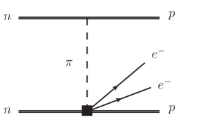
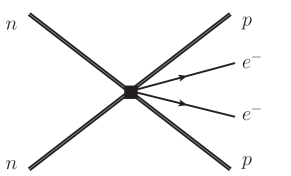
Figure 2: Hadron-level Feynman diagrams for $0\nu\beta\beta$ decay induced by the LNV operators $\pi NNee$ (left) and $NNNNee$ (right), which are denoted by the black squares.

In chiral perturbation theory the quark-lepton operators are mapped onto hadron-lepton operators defined below the scale $\Lambda_{\chi}\sim 1\leavevmode\nobreak\ \text{GeV}$, with the non-perturbative QCD dynamics encoded by low-energy constants (LECs) Bernard:1995dp ; Gasser:1983yg .

In several ways the behavior of the vector operators in chiral perturbation theory is in striking contrast to that of scalar operators. For vector operators, their lowest order local interaction with pions is of the form $(\pi\partial_{\mu}\pi)\overline{e}\gamma^{\mu}\gamma_{5}e^{c}$ which, after using the pion equations of motion, is $\pi\pi ee$, but importantly suppressed by a factor of $m_{e}$ and negligible Prezeau:2003xn ; Graesser:2016bpz - for further details see Appendix A. Unlike scalar operators, vector operators do not induce any operators at LO in the chiral power counting. The leading contribution of the vector operators $O_{6,7,8,9}^{\mu\prime}\bar{e}\gamma_{\mu}\gamma_{5}e^{c}$ to the $0\nu\beta\beta$-decay amplitude instead arises from their mapping onto the hadronic operators $\pi NNee$ and $NNNNee$  Prezeau:2003xn ; Graesser:2016bpz ; Cirigliano:2018yza which are at NLO and N²LO in Weinberg’s power counting Weinberg:1990rz ; Weinberg:1991um , respectively. While requiring that the amplitude is regulator independent implies that the LECs for these two operators are related, in the case of vector operators, no “promotion” of the $NNNNee$ operators to lower chiral order is needed, and at least for these vector operators, Weinberg’s power counting appears correct Cirigliano:2018yza ; Cirigliano:2019vdj . In the case of vector operators then, the $\pi NNee$ and $NNNNee$ operators make comparable contributions to the $0\nu\beta\beta$-decay amplitude. The $0\nu\beta\beta$-decay rate however has a sizable uncertainty due to the unknown values of these LECs, as is illustrated in Fig. 3.

In heavy-baryon chiral perturbation theory Jenkins:1990jv the effective Lagrangian for the leading hadron-level LNV interactions $\pi NNee$ and $NNNNee$ is given by Cirigliano:2018yza

$$\mathcal{L}^{\rm vector}_{\text{eff}} = \mathcal{L}^{\rm vector}_{\pi N}+\mathcal{L}^{\rm vector}_{NN}\leavevmode\nobreak\ ,$$ (14)

$$\mathcal{L}^{\rm vector}_{\pi N} = \frac{1}{v^{5}}\sqrt{2}g_{A}F_{\pi}\bar{p}S^{\alpha}\cdot\partial_{\alpha}\pi^{-}n\Big{[}g_{V}^{\pi N}C_{V}^{(9)}+\tilde{g}_{V}^{\pi N}\tilde{C}_{V}^{(9)}\Big{]}\times v^{\mu}\bar{e}\gamma_{\mu}\gamma_{5}e^{c}\leavevmode\nobreak\ ,$$ (15)

$$\mathcal{L}^{\rm vector}_{NN} = \frac{1}{v^{5}}(\bar{p}n)(\bar{p}n)\Big{[}g_{6}^{NN}C_{V}^{(9)}+g_{7}^{NN}\tilde{C}_{V}^{(9)}\Big{]}\times v^{\mu}\bar{e}\gamma^{\mu}\gamma_{5}e^{c}\leavevmode\nobreak\ ,$$ (16)

where $F_{\pi}=91.2\leavevmode\nobreak\ \text{MeV}$, $g_{A}=1.27$, and $S^{\alpha}$ and $v^{\mu}$ are the nucleon spin and velocity. The coefficients

$$C_{V}^{(9)} =C_{6}^{\prime}(m_{0})+C_{8}^{\prime}(m_{0})\;,$$

$$\tilde{C}_{V}^{(9)} =C_{7}^{\prime}(m_{0})+C_{9}^{\prime}(m_{0})\;\leavevmode\nobreak\ .$$ (17)

The LECs $g_{V}^{\pi N},\tilde{g}_{V}^{\pi N},g_{6}^{NN},g^{NN}_{7}=\mathcal{O}(1)$ in the naïve dimensional analysis (NDA) Manohar:1983md ; Weinberg:1989dx , and little is known about them. Inspecting the numerical solution to the RG equations (12) and (13), one finds $C_{V}^{(9)}=1.43v^{5}/(2\Lambda^{5})[C_{Qu1}(\Lambda)+C_{Qd1}(\Lambda)]$ – so that this Wilson coefficient has an $\mathcal{O}(1)$ enhancement at low scales – and a small non-vanishing $\tilde{C}_{V}^{(9)}$ has been generated.

In Fig. 2 we show the Feynman diagrams for the $0\nu\beta\beta$ decay at hadron-level, that is the transition $nn\to ppee$, which are induced by the NLO operators $\pi NNee$ and N²LO operators $NNNNee$. In chiral power counting, the transition amplitudes of these two diagrams are at the same order. For the vector operators consider here, the amplitude for nuclear $0\nu\beta\beta$ decay $0^{+}\to 0^{+}$ is Cirigliano:2018yza

$$\mathcal{A}_{\text{vector}}=\dfrac{g_{A}^{2}G_{F}^{2}m_{e}}{\pi R_{A}}\mathcal{A}_{M}\bar{u}(k_{1})\gamma_{0}\gamma_{5}C\bar{u}^{T}(k_{2})\;,$$ (18)

where $k_{1}$ and $k_{2}$ are the momenta of the emitted electrons, $G_{F}$ is Fermi coupling constant, the radius $R_{A}=1.2A^{1/3}$ fm with $A$ the number of nucleons of nucleus, and the reduced amplitude is given by

$$\mathcal{A}_{M} = \dfrac{m_{\pi}^{2}}{m_{e}v}\left[\dfrac{1}{2}(g_{V}^{\pi N}C_{V}^{(9)}+\tilde{g}_{V}^{\pi N}\tilde{C}_{V}^{(9)})M_{P,sd}-\frac{2}{g^{2}_{A}}\left(g^{NN}_{6}C^{(9)}_{V}+g^{NN}_{7}\tilde{C}^{(9)}_{V}\right)M_{F,sd}\right]$$ (19)

with $M_{P,sd}\equiv(M_{GT,sd}^{AP}+M_{T,sd}^{AP})$, where the basic NMEs $M_{GT,sd}^{AP}=-2.80$, $M_{T,sd}^{AP}=-0.92$ and $M_{F,sd}=-1.53$ for ¹³⁶Xe calculated using the quasi-particle random phase approximation (QRPA) Hyvarinen:2015bda . The reader is referred to Ref. Cirigliano:2017djv ; Cirigliano:2018yza for definitions of these basic NMEs. The inverse half-life of the $0\nu\beta\beta$ decay is expressed as

$$\left(T_{1/2}^{0\nu}\right)^{-1}=g_{A}^{4}G_{09}|\mathcal{A}_{M}|^{2}\;,$$ (20)

where the phase space factor $G_{09}=2.8\times 10^{-14}\leavevmode\nobreak\ \text{year}^{-1}$ for ¹³⁶Xe Horoi:2017gmj , following a trivial rescaling as discussed in Cirigliano:2018yza ; Cirigliano:2017djv ; see also Ref. Stefanik:2015twa ; Doi:1985dx . Three-body nucleon interactions such as $NNNNNNee$ contributing to $0^{+}\rightarrow 0^{+}$ are expected to contribute at higher-order in the Weinberg power counting and are not considered here.

As discussed above, the vector operators $O_{6,7,8,9}^{\mu\prime}\bar{e}\gamma_{\mu}\gamma_{5}e^{c}$ are mapped onto the operators $\pi NNee$ and $NNNNee$, whose contributions are suppressed in chiral power counting. This can be seen in Eq. (19) with the amplitude $\mathcal{A}_{M}$ being proportional to $m_{\pi}^{2}$, while amplitudes for the LO hadron-lepton operators are proportional to $\Lambda_{\chi}^{2}$ Prezeau:2003xn ; Graesser:2016bpz ; Cirigliano:2018yza . An explicit UV completion of these scalar quark-lepton operators can be found in Ref. Li:2021fvw .

As an aside, one may naïvely expect that, in the absence of any underlying model and consequently no linear ordering of the magnitudes of the Wilson coefficients of these operators, the vector operators are quantitatively less important than scalar operators in $0\nu\beta\beta$ decay due to the suppression of the $0\nu\beta\beta$-decay amplitude by a factor of $(\Lambda_{\chi}/m_{\pi})^{2}\sim 60$. However, this level of suppression may not be realized in practice. To illustrate, consider a comparison with the $0\nu\beta\beta$-decay amplitude $(\mathcal{A}_{\text{scalar}})$ induced by scalar operators. It turns out that this suppression is sensitive to the size of certain unknown LECs as well as NMEs. To see why, first consider the limit where the unknown LECs for operators $NNNNee$ contributing to $\mathcal{A}_{\text{scalar}}$ follow the Weinberg power counting expectation of $\mathcal{O}(1)$, then

$$\frac{\mathcal{A}_{\text{vector}}}{\mathcal{A}_{\text{scalar}}}\simeq\frac{m^{2}_{\pi}}{m^{2}_{N}}\frac{M_{P,sd}}{M_{PS,sd}}\leavevmode\nobreak\ ,$$ (21)

where $m_{N}\sim\Lambda_{\chi}$ is the nucleon mass and $\mathcal{A}_{\text{scalar}}$ arises from the LO pion-exchange interaction. Here $M_{PS,sd}$ is a NME that appears in the expression for $\mathcal{A}_{\text{scalar}}$; more details on each can be found in Appendix A. As shown in Appendix A, the ratio of NMEs is about $6-8$, across a variety of isotopes and methods for estimating their values. Thus, the naïvely expected suppression may too severe by nearly an order of magnitude. In addition, recent work suggests that the the LECs for the $NNNNee$ arising from the scalar operators may be considerably larger than $\mathcal{O}(1)$ Cirigliano:2018hja ; Cirigliano:2018yza ; Cirigliano:2019vdj ; Cirigliano:2020dmx ; Cirigliano:2021qko – for more details the reader is referred to Appendix A. The $NNNNee$ contribution to $\mathcal{A}_{\text{scalar}}$ involves yet another NME, further clouding the estimated magnitude of the full scalar amplitude.

Substituting the values of the phase space factor, NMEs and the other constants into Eq. (20), we obtain

$$(T_{1/2}^{0\nu})^{-1} \simeq 6.0\times 10^{-22}\big{[}(0.98g_{V}^{\pi N}-g_{6}^{NN})-(0.069\tilde{g}_{V}^{\pi N}-0.070g_{7}^{NN})\big{]}^{2}$$

$$\quad\times\left|y_{e\Psi}(y_{qu}+y_{qd})\lambda_{ed}\lambda_{u\Psi}\right|^{2}\times\left(\dfrac{\text{TeV}^{5}}{m_{S}^{2}m_{R}^{2}m_{\Psi}}\right)^{2}\leavevmode\nobreak\ \text{year}^{-1}\;,$$ (22)

where all of the masses are normalized by the scale of $1\leavevmode\nobreak\ \text{TeV}$.

The most stringent $0\nu\beta\beta$-decay limit comes from the experiment KamLAND-Zen KamLAND-Zen:2016pfg : $T_{1/2}^{0\nu}>1.07\times 10^{26}\leavevmode\nobreak\ \text{year}$ at 90% confidence level (C.L.). The constraint from the final results of GERDA experiment GERDA:2020xhi is slightly weaker. There exist a number of planned experiments at the ton-scale Kharusi:2018eqi ; Abgrall:2017syy ; CUPIDInterestGroup:2019inu ; Paton:2019kgy ; Chen:2016qcd ; Adams:2020cye that aim to improve the half-life sensitivity by about 2 orders of magnitude, reaching $T_{1/2}^{0\nu}>10^{28}\leavevmode\nobreak\ \text{year}$ at 90% C.L. From Eq. (2.1), we thus infer that future ton-scale $0\nu\beta\beta$-decay experiments are able to probe TeV-scale LNV with the masses $m_{S}=m_{R}=m_{\Psi}=1\leavevmode\nobreak\ \text{TeV}$ and the couplings $|y_{e\Psi}(y_{qu}+y_{qd})\lambda_{ed}\lambda_{u\Psi}|\gtrsim(3-9)\times 10^{-3}$ for $g_{V}^{\pi N}=\tilde{g}_{V}^{\pi N}=1$ and $g^{NN}_{6}=g^{NN}_{7}=\pm 1/2$. In Fig. 3, we show for three sets of assumed values for these low-energy constants, the half-lives of $0\nu\beta\beta$ decay for ¹³⁶Xe as a function of the LNV scale. Clearly, we can see that typically the LNV scale up to around $4.5-6\leavevmode\nobreak\ \text{TeV}$ for the Wilson coefficients $C_{Qu1}+C_{Qd1}=1$ is in the reach of next-generation ton-scale $0\nu\beta\beta$-decay experiments. The same figure also illustrates that the sensitivity of the inferred LNV scale to these LECs is sizable.

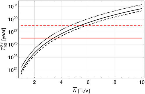
Figure 3: Half-lives of $0\nu\beta\beta$ decay as a function of the effective LNV scale $\overline{\Lambda}\equiv\Lambda/\left|C_{Qu1}+C_{Qd1}\right|^{1/5}$. The solid black curve is obtained with $g_{V}^{\pi N}=\tilde{g}_{V}^{\pi N}=1$ and $g^{NN}_{6}=g^{NN}_{7}=0$. The dotted (dashed) black curve is obtained with the same settings of $g_{V}^{\pi N}$, $\tilde{g}_{V}^{\pi N}$ but with $g^{NN}_{6}=g^{NN}_{7}=1/2$ $(-1/2)$. The solid red and dashed red lines correspond to the constraints on the half-life in KamLAND-Zen and future ton-scale experiments for ¹³⁶Xe.

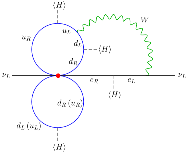
Figure 4: The LNV vector operators contribute to neutrino masses at three-loop or higher order, and are completely negligible. Shown here is a typical three-loop Feynman diagram contributing to the neutrino mass. The red dot depicts the dimension-9 operators in Eq. (2.2). The analogous diagram in the simplified model is shown in Fig. 14 of Appendix B.

2.2 Neutrino masses: dimension-9 operators

Before closing this section, it is interesting to discuss the connection in this model between $0\nu\beta\beta$ decay and neutrino masses. On general grounds, the Schechter-Valle theorem Schechter:1981bd implies that the observation of $0\nu\beta\beta$ decay implies the existence of a light neutrino Majorana mass term. For the model of interest here, the $0\nu\beta\beta$-decay operators can induce Majorana neutrino masses at loop level. It is instructive to consider this connection after integrating out the heavy degrees of freedom. Retaining only the light degrees of freedom, we obtain the loop-induced Majorana mass from diagrams such as Fig. 4. In the simplified model neutrino masses are generated at three-loop level as briefly discussed in Appendix B. The red dot in Fig. 4 depicts the effective operators in the form of

$$\frac{C_{Qu1}}{\Lambda^{5}}(\bar{u}_{R}u_{L})(\bar{u}_{R}\gamma_{\mu}d_{R})(\bar{e}_{R}\gamma^{\mu}\nu_{L}^{c})\;,$$

$$\frac{C_{Qd1}}{\Lambda^{5}}(\bar{d}_{L}d_{R})(\bar{u}_{R}\gamma_{\mu}d_{R})(\bar{e}_{R}\gamma^{\mu}\nu_{L}^{c})\;.$$ (23)

In the SMEFT, they arise from the $\nu-$component of the $SU(2)_{L}\times U(1)_{Y}$ invariant dimension-9 effective operators in Eq. (5). The contribution of these operators to the neutrino mass is highly suppressed by three insertions of the light quark masses and one of the electron mass, as well as by the loop factors, and is estimated as

$$m_{\nu} \sim \frac{m_{d}m_{u}m_{e}}{(16\pi^{2})^{3}}\frac{\Lambda_{\text{UV}}^{2}}{\Lambda^{5}}\left(m_{u}C_{Qu1}+m_{d}C_{Qu2}\right)$$ (24)

$$\simeq 10^{-24}\text{MeV}\left(\frac{m^{3}_{u,d}m_{e}}{\text{MeV}^{4}}\right)\left(\frac{\Lambda_{\text{UV}}}{\text{1 TeV}}\right)^{2}\left(\frac{\text{1 TeV}}{\Lambda}\right)^{5}\;,$$

which is completely negligible compared to the actual neutrino masses. Here $\Lambda_{\text{UV}}$ is an UV cutoff, with $\Lambda_{\text{UV}}\sim\Lambda$. Two powers of $\Lambda_{\text{UV}}$ arise from the quadratic divergence in the “bubble” loop of light quarks appearing below the “horizontal line” in Fig. 4. (In dimensional regularization two powers of the light quark masses would appear instead.) In obtaining this estimate we have defined $\Lambda^{5}\equiv(m^{2}_{S}m^{2}_{R}m_{\Psi})$ and set equal to one the product of Yukawa couplings appearing in the Wilson coefficients $C_{Qu1}$ and $C_{Qd1}$: $\frac{1}{2}y_{e\Psi}\lambda_{ed}\lambda_{u\Psi}y_{qu}\equiv\frac{1}{2}y_{e\Psi}\lambda_{ed}\lambda_{u\Psi}y_{qd}\equiv 1.$ The simplified model presented here cannot generate the observed neutrino masses, which therefore must arise from some other source.

We end by returning to the Schechter-Valle “black box” theorem Schechter:1981bd . It is noted that the contribution to Majorana neutrino masses arising from an insertion of the $0\nu\beta\beta$ decay “black-box operator” occurs at four-loop level. The induced shift in the Majorana neutrino mass, derived using the experimental limit $T^{0\nu}_{1/2}>1.07\times 10^{26}$ year, is roughly $2\times 10^{-28}$ eV Duerr:2011zd . Here we have updated the numerical results of Ref. Duerr:2011zd to reflect the more recent KamLAND-Zen limit KamLAND-Zen:2016pfg . This value is much smaller than the direct contribution to neutrino masses arising in the simplified model considered here.

2.3 Dimension-7 operator

Here we consider the effects of the interaction

$$y_{e\Psi}^{\prime}\bar{\Psi}_{L}He_{R}\leavevmode\nobreak\$$ (25)

on $0\nu\beta\beta$ decay. This interaction appears in the last line of the Lagrangian in Eq. (2), and is allowed by all symmetries. It does not contribute to the LNV dimension-9 operators, but its presence does generate a LNV dimension-7 operator above the electroweak scale. The Yukawa coupling $y_{e\Psi}^{\prime}$ has zero lepton number.

To see that it cannot be forbidden by any symmetry, note that the model already has Yukawa couplings of $S$ to the SM quarks. Under any discrete symmetry $S$ and $H$ must have the same charge, which means we cannot distinguish $S$ from $H$. Thus if we have $\bar{\Psi}_{L}Se_{R}$ in the Lagrangian we cannot forbid $\bar{\Psi}_{L}He_{R}$. This operator cannot be forbidden by any $Z_{N}$ discrete symmetry.

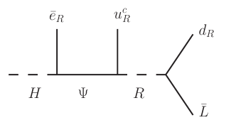
Figure 5: Quark-level Feynman diagram that induce $\Delta L=2$ dimension-7 $0\nu\beta\beta$-decay operator $O_{Leu\bar{d}H}$ at low energies.

Integrating out $S$ and $R$ at tree-level gives the following new contribution to the effective theory below that mass scale,

$$\mathcal{L}_{{\rm SMEFT}}^{(7)}= \dfrac{1}{\Lambda^{3}}C_{Leu\bar{d}H}O_{Leu\bar{d}H}+\text{h.c.}\;,$$ (26)

where the dimension-7 operator is given by

$$O_{Leu\bar{d}H}=(\bar{u}_{R}\gamma_{\mu}d_{R})(\bar{e}_{R}\gamma^{\mu}L^{c})H^{*}$$ (27)

with a Wilson coefficient

$$\dfrac{C_{Leu\bar{d}H}}{\Lambda^{3}}=\dfrac{1}{2}\dfrac{y_{e\Psi}^{\prime}\lambda_{ed}\lambda_{u\Psi}}{m_{R}^{2}m_{\Psi}}$$ (28)

The Feynman diagram generating this effective interaction is shown in Fig. 5. Note that this Wilson coefficient depends on the same combination of Yukawa couplings $(\lambda_{ed}\lambda_{u\Psi})$ that appears in the Wilson coefficients of the dimension-9 operators. Of course, here $y_{e\Psi}^{\prime}$ also occurs, which does not appear in the dimension-9 Wilson coefficients.

The operator $O_{Leu\bar{d}H}$ is proportional to a current of quarks, so the QCD RG evolution of this operator is trivial. After the electroweak symmetry breaking, the Higgs doublet $H$ develops the vev $\langle H\rangle=v/\sqrt{2}$, and the following effective Lagrangian in the LEFT is obtained

$$\mathcal{L}_{{\rm LEFT}}^{(6)}=\dfrac{1}{v^{2}} C^{(6)}_{\text{VR}}O^{(6)}_{\text{VR}}+\text{h.c.}\;,$$ (29)

where the dimension-6 operator is

$$O^{(6)}_{\text{VR}}=(\bar{u}_{R}\gamma_{\mu}d_{R})(\bar{e}_{R}\gamma^{\mu}\nu^{c})\;.$$ (30)

and the Wilson coefficient is given by

$$\dfrac{1}{v^{3}}C^{(6)}_{\text{VR}}= \dfrac{1}{\sqrt{2}\Lambda^{3}}C^{*}_{Leu\bar{d}H}\;.$$ (31)

Due to the presence of the neutrino, this interaction make a long-distance contribution to $0\nu\beta\beta$ decay as shown in Fig. 6.

Figure 6: Hadron-level Feynman diagram for $0\nu\beta\beta$ decay, induced by the LNV operator $np\overline{e}\nu^{c}$ denoted by the black square. The other vertex denotes the single $\beta$ decay operator from SM interactions.

Below the scalar $\Lambda_{\chi}\sim 1\leavevmode\nobreak\ \text{GeV}$, the quark-lepton operator are mapped onto hadron-lepton operators. Up to NLO in chiral expansion, the resulting one-body current for single $\beta$ decay was shown explicitly in Ref. Cirigliano:2017djv .

At LO in the Weinberg power counting, the dimension-6 operator $O^{(6)}_{\text{VR}}$ makes a vanishing contribution to $0\nu\beta\beta$ decay. The first non-vanishing contribution is obtained by expanding the one-body vector and axial currents to NLO Cirigliano:2017djv . The contribution of the dimension-6 operator $O^{(6)}_{\text{VR}}$ to the amplitude for $0^{+}\to 0^{+}$ is given by Cirigliano:2017djv ; Cirigliano:2018yza

$$\mathcal{A}_{\text{VR}}=\dfrac{g_{A}^{2}G_{F}^{2}m_{e}}{\pi R_{A}}\left[\mathcal{A}_{E}\bar{u}(k_{1})\gamma_{0}C\bar{u}^{T}(k_{2})\dfrac{E_{1}-E_{2}}{m_{e}}+\mathcal{A}_{m_{e}}\bar{u}(k_{1})C\bar{u}^{T}(k_{2})\right]\;,$$ (32)

where $E_{1}$ and $E_{2}$ are the energies of the emitted electrons and the reduced amplitudes are

$$\mathcal{A}_{E}=C^{(6)}_{\text{VR}}M_{E,R}\;,\quad\mathcal{A}_{m_{e}}=C^{(6)}_{\text{VR}}M_{m_{e},R}\;,$$ (33)

and the NMEs

$$M_{E,R} = -\dfrac{1}{3}\left[\dfrac{g^{2}_{V}}{g^{2}_{A}}M_{F}-\dfrac{1}{3}\left(2M^{AA}_{GT}+M^{AA}_{T}\right)\right]\;,$$

$$M_{m_{e},R} = \dfrac{1}{6}\left[\dfrac{g^{2}_{V}}{g^{2}_{A}}M_{F}+\dfrac{1}{3}\left(M^{AA}_{GT}-4M^{AA}_{T}\right)+3(M^{AP}_{GT}+M^{PP}_{GT}+M^{AP}_{T}+M^{PP}_{T})\right]\;.$$ (34)

Here, $g_{V}=1$, and the six long-range NMEs are given by $M_{F}=-0.89$, $M^{AA}_{GT}=3.16$, $M^{AP}_{GT}=-1.19$, $M^{PP}_{GT}=0.39$, $M^{AP}_{T}=-0.28$, and $M^{PP}_{T}=0.09$ for ¹³⁶Xe calculated using the QRPA method Hyvarinen:2015bda . The NME $M^{AA}_{T}$ cannot be extracted from current calculations of light and heavy neutrino Majorana mass contributions to $0\nu\beta\beta$ decays of current experimental interest. Here we set it to zero as it is expected to be small compared to the other NMEs. With these as input, $M_{E,R}=0.89$ and $M_{m_{e},R}=-0.41$, again for ¹³⁶Xe.

The amplitude is proportional to the outgoing electron energies or the electron mass and therefore highly suppressed. In the Weinberg power counting three-body nucleon interactions and loops of pions are expected to make comparable contributions. As a result, the limit and projection obtained below should be viewed as an order-of-magnitude estimate Cirigliano:2017djv .

The inverse half-life is given by Cirigliano:2017djv

$$\left(T_{1/2}^{0\nu}\right)^{-1}=g_{A}^{4}\left[4G_{02}|\mathcal{A}_{E}|^{2}-4G_{03}\text{Re}\left(\mathcal{A}_{m_{e}}\mathcal{A}_{E}\right)+2G_{04}|\mathcal{A}_{m_{e}}|^{2}\right]$$ (35)

with the phase space factors $G_{02}=3.2\times 10^{-14}$ year^-1, $G_{03}=0.86\times 10^{-14}$ year^-1, and $G_{04}=1.2\times 10^{-14}$ year^-1 for ¹³⁶Xe. Substituting for $C^{(6)}_{\text{VR}}$, the NMEs, and the phase space factors, gives

$$\left(T_{1/2}^{0\nu}\right)^{-1} = 8.6\times 10^{-18}|y_{e\Psi}^{\prime}\lambda_{ed}\lambda_{u\Psi}|^{2}\times\left(\dfrac{\text{TeV}^{3}}{m_{R}^{2}m_{\Psi}}\right)^{2}\leavevmode\nobreak\ \text{year}^{-1}\;.$$ (36)

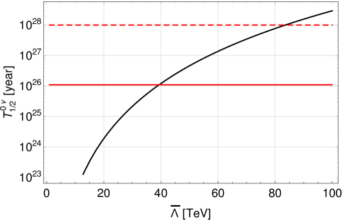
Figure 7: Half-lives of $0\nu\beta\beta$ decay as a function of the effective LNV scale $\overline{\Lambda}\equiv\Lambda/\left|C_{Leu\bar{d}H}\right|^{1/3}$. The solid red and dashed red lines correspond to the constraints on the half-life in the KamLAND-Zen and future ton-scale experiments for ¹³⁶Xe.

The Kamland-Zen limit of $T_{1/2}^{0\nu}>1.07\times 10^{26}$ year gives a constraint of $|y_{e\Psi}^{\prime}\lambda_{ed}\lambda_{u\Psi}|<3.3\times 10^{-5}$ for $m_{R}=m_{\Psi}=1$ TeV. Setting the Yukawa couplings equal to one, this bound translates into a bound on $\Lambda\equiv(m^{2}_{R}m_{\Psi})^{1/3}\buildrel>\over{{}_{\sim}}40$ TeV. Current and projected limits are shown in Fig. 7, where we can see that future ton-scale experiments are sensitive to the LNV scale up to $90\leavevmode\nobreak\ \text{TeV}$ for the Wilson coefficient $C_{Leu\bar{d}H}=1$.

One can see that $0\nu\beta\beta$ decay is more sensitive to the dimension-7 operator $O_{Leu\bar{d}H}$ compared to the dimension-9 vector operators. Following Refs. Cirigliano:2017djv ; Cirigliano:2018yza , this can be understood in chiral power counting. Denoting $\epsilon_{\chi}=q/\Lambda_{\chi}$ with $q\sim m_{\pi}$ the typical momentum transfer of $0\nu\beta\beta$ decay, then the typical outgoing electron energies scale as $E\sim\hbox{MeV}\sim\Lambda_{\chi}\epsilon_{\chi}^{3}$. Since the reduced amplitudes $m_{e}\mathcal{A}_{E}$ and $m_{e}\mathcal{A}_{m_{e}}$ induced by $O_{\text{VR}}^{(6)}$ are proportional to the electron energies, they scale as $\Lambda_{\chi}\epsilon_{\chi}^{3}$. In contrast, $m_{e}\mathcal{A}_{M}$ induced by the dimension-9 vector operators scales as $\Lambda_{\chi}^{2}\epsilon_{\chi}^{2}/v$. Although all of them are chirally suppressed, $\mathcal{A}_{M}$ is smaller than $\mathcal{A}_{E}$ and $\mathcal{A}_{m_{e}}$ by a factor of $\Lambda_{\chi}/(v\epsilon_{\chi})\simeq 0.03$.

The existence of the Yukawa interaction $y_{e\Psi}^{\prime}\bar{\Psi}_{L}He_{R}$ would also contribute to the deviation from unitarity of the Pontecorvo-Maki-Nakagawa-Sakata matrix and mass mixing of charged leptons with more phenomenological implications and constraints. However, since the LHC searches considered in the next section are insensitive to this interaction, we simply assume that it is suppressed, which might be realized in UV theories, and focus on the interplay of chirally suppressed $0\nu\beta\beta$ decay induced by the dimension-9 vector operators and LHC searches.

2.4 Neutrino masses: dimension-7 operators

This discussion closes with some comments about neutrino masses. Like the dimension-9 operator previously discussed in Section 2.1, the dimension-7 operator Eq. (26) also generates neutrino masses at higher loop order. In particular, a neutrino mass is first generated at two-loops and is finite. It is highly suppressed due to one electron mass and two light quark mass insertions, and one estimates that

$$m_{\nu} \sim \frac{C_{Leu\bar{d}}}{(16\pi^{2})^{2}}\frac{m_{d}m_{u}m_{e}}{\Lambda^{3}}v$$ (37)

$$\simeq 10^{-17}C_{Leu\bar{d}}\text{MeV}\left(\frac{m_{u}m_{d}m_{e}}{\text{MeV}^{3}}\right)\left(\frac{\text{1 TeV}}{\Lambda}\right)^{3}\;,$$

which is completely negligible. Consequently, the observed values of the neutrino masses do not constrain the size of this Wilson coefficient.

3 LHC searches

We will investigate the complementary test of TeV-scale LNV in our simplified model using LHC searches. The process with a pair of first generation leptons with the same charge ($e^{\pm}e^{\pm}$) and at least two jets would provide a clear sign of LNV at the LHC. Searches for this same-sign dilepton plus dijet signal have thus far yielded null results, leading to constraints on different models for TeV-scale LNV. We analyze the corresponding implications for our simplified model below. Additionally, searches for leptoquarks as well as those for dijet resonances, which do not rely on LNV signatures, can also be used to extend the sensitivities to the masses and couplings of new particles in our simplified model.

In this section, we will reinterpret the existing searches, which are performed at the 13 TeV LHC with integrated luminosities of $\sim 40\leavevmode\nobreak\ \text{fb}^{-1}-140\leavevmode\nobreak\ \text{fb}^{-1}$, in terms of the corresponding LNV and lepton number conserving processes generated in our model, then make projections for the high-luminosity LHC (HL-LHC) with the integrated luminosity of $3\leavevmode\nobreak\ \text{ab}^{-1}$. In all of our projections for exclusion and discovery at the HL-LHC, we make the strong assumption that the selection cuts and efficiencies remain unchanged from those in existing searches. The reaches presented here might be improved with an optimization of cuts.

Note that both $y_{qu}$ and $y_{qd}$ terms in Eq. (2) can contribute to the scalar production at the LHC, which do not interfere. For the charged scalar $S^{\pm}$, their contributions to the production cross section are the same if $y_{qu}=y_{qd}$. For the neutral scalar $S^{0}$, however, the contribution to the production cross section from the $y_{qu}$ term is larger than that from the $y_{qd}$ term, since $u$-quark parton distribution function (PDF) is typically about two times larger than $d$-quark PDF for the Bjorken $x\sim m_{S}/\sqrt{s}$, which is around $0.1-0.2$. Here, $\sqrt{s}=13\leavevmode\nobreak\ \text{TeV}$ is the center-of-mass energy of the LHC. Consequently, the constraints from dijet search in case of non-vanishing $y_{qd}$ is relatively weaker than that for non-vanishing $y_{qu}$.

Besides, different from the $0\nu\beta\beta$-decay half-life that depends on $(y_{qu}+y_{qd})^{2}$, there is no interference between the contributions from the $y_{qu}$ and $y_{qd}$ terms to the production cross sections of $pp\to S^{\pm},S^{0}$. Hereafter, to simplify the presentation of our analysis, we assume $y_{qu}=0$ and $y_{qd}\neq 0$, and study the interplay of LHC searches and $0\nu\beta\beta$ decay. Our conclusions would be qualitatively similar if $y_{qd}=0$ and $y_{qu}\neq 0$ were assumed instead.

3.1 Leptoquark searches

Direct search for pairs of first-generation leptoquarks by the ATLAS collaboration at the 13 TeV LHC with an integrated luminosity of $139\leavevmode\nobreak\ \text{fb}^{-1}$ has excluded the leptoquark mass region below 1.8 TeV Aad:2020iuy . To make a conservative projection for the future sensitivity to leptoquarks, we assume that both observed upper limit on the number of signal events and the number of the background events in Ref. Aad:2020iuy scale with the integrated luminosity, and obtain that the lower limit on the leptoquark mass at the LHC is about $2\leavevmode\nobreak\ \text{TeV}$ with an integrated luminosity of $1\leavevmode\nobreak\ \text{ab}^{-1}$. These constraints become weaker if the decay branching ratio of leptoquark into electron $e^{+}/e^{-}$ and quark is less than 1.

In the analysis of the leptoquark search Aad:2020iuy , a pair of opposite-sign electrons $e^{+}e^{-}$ and at least two jets are required in the final state. In addition, the pairs of electron and jet closest in the invariant mass must satisfy $m^{\text{asym}}_{ej}\equiv(m_{ej}^{\text{max}}-m_{ej}^{\text{min}})/(m_{ej}^{\text{max}}+m_{ej}^{\text{min}})<0.2$, where $m_{ej}^{\text{max}}$ and $m_{ej}^{\text{min}}$ denote the larger and smaller of the two electron-jet invariant masses. The upper limits on $\sigma\times\mathcal{B}\times A$ for each leptoquark mass are derived by performing fits to the distribution of $m^{\text{mean}}_{ej}$, which is defined as $m^{\text{mean}}_{ej}\equiv(m_{ej}^{\text{max}}+m_{ej}^{\text{min}})/2$. Here, $\sigma$ denotes the leptoquark pair production cross section, $\mathcal{B}$ is the product of the decay branching ratios of intermediate particles, and $A$ describes the overall acceptance.

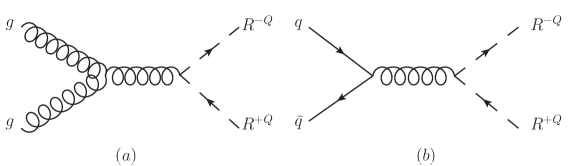
Figure 8: Representative Feynman diagrams for the parton-level pair production of leptoquarks $(R^{\pm Q})$. Here, $g$ denotes a gluon $q$ denotes a quark, and the electric charge $Q=2/3,1/3$.

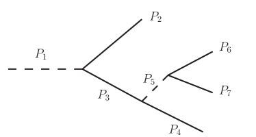
Figure 9: Feynman diagram for the cascade decays of leptoquarks. The labels $P_{1},\ldots,P_{7}$ denote the possible particles in the chain, which are specified in Tab. 1.

Table 1: The cascade decays of leptoquarks in the presence of $\Psi$.

$P_{1}$	$P_{2}$	$P_{3}$	$P_{4}$	$P_{5}$	$P_{6}$	$P_{7}$
${R}^{2/3}$	$u$	$\Psi^{0}$	$\bar{u}$	${R}^{2/3}$	$d$	$e^{+}$
${R}^{2/3}$	$u$	$\Psi^{0}$	$e^{-}$	$S^{+}$	$u$	$\bar{d}$
${R}^{1/3}$	$\bar{u}$	$\Psi^{+}$	$e^{+}$	$S^{0}$	$d$	$\bar{d}$

The signal process $pp\to{R}^{+2/3}{R}^{-2/3}$, ${R}^{2/3}\to e^{+}d$, ${R}^{-2/3}\to e^{-}\bar{d}$ has the same acceptance $A$ as Ref. Aad:2020iuy . Thus the upper limit on $\sigma\times\mathcal{B}$ reported in Ref. Aad:2020iuy can be directly applied to this signal process. However, this conclusion is not true for other signal processes due to different cut acceptances. To be more specific, in our simplified model the leptoquark ${R}$ can also have a cascade decay if $m_{R}>m_{\Psi}$. In Figs. 8 and 9, we show schematic Feynman diagrams for the pair production and cascade decays of leptoquarks.

In fact, for the other leptoquark pair production processes such as $pp\to{R}^{+2/3}{R}^{-2/3}$, ${R}^{-2/3}\to e^{-}\bar{d}$, ${R}^{+2/3}\to\Psi^{0}u,$ $\Psi^{0}\to e^{+}\bar{u}d$, and $pp\to{R}^{+1/3}{R}^{-1/3}$, ${R}^{+1/3}\to\Psi^{+}\bar{u}$, ${R}^{-1/3}\to\Psi^{-}u$, $\Psi^{\pm}\to e^{\pm}d\bar{d}$, after imposing the cut $m^{\text{asym}}_{ej}<0.2$ the efficiencies and the values of $m^{\text{mean}}_{ej}$ are smaller, since there are more jets in the final state. This leads to a smaller overall acceptance $A$. Finally, it is noted that in our model the processes $pp\to e^{+}\Psi^{0}$, $\Psi^{0}\to e^{-}u\bar{d}$ and $pp\to e^{-}\bar{\Psi}^{0}$, $\bar{\Psi}^{0}\to e^{+}d\bar{u}$ also contribute to our reinterpretion of the leptoquark search Aad:2020iuy , but their contributions are substantially reduced by the selection cut on $m_{ej}^{\text{asym}}$.

After taking into account all of the signal processes with the possible decays of $R$, and deducing the corresponding acceptance, the lower bound on the leptoquark mass is expected to be smaller than that in Ref. Aad:2020iuy . Instead of reanalyzing the fits for all of these signals, we will assume conservatively the leptoquark mass $m_{R}=2\leavevmode\nobreak\ \text{TeV}$.

The leptoquark pair production $pp\to{R}^{+1/3}{R}^{-1/3}$ can also give signatures of jets $+$ MET (monojet), jets $+$ $e^{\pm}$ $+$ MET, where the missing energy (MET) comes from neutrino(s) in $R^{+1/3}\to\bar{d}\nu$ and/or $R^{-1/3}\to d\bar{\nu}$ and $e^{\pm}$ come from the cascade decay of $R^{\pm 1/3}$. However, due to low trigger efficiencies of these signals the constraints are expected to be very weak, and will not be considered hereafter.

Finally, it is worth noting that other searches for first-generation leptoquark may give constraints comparable to the pair production with the assumption that both the leptoquark coupling $\lambda_{ed}$ and decay branching ratio are equal to 1. In Ref. Khachatryan:2015qda , a search for the single production of leptoquark was performed by the CMS Collaboration at the 8 TeV LHC with an integrated luminosity of $19.6\leavevmode\nobreak\ \text{fb}^{-1}$. The recast and projection of this search with the same selection cuts being imposed Schmaltz:2018nls show that $m_{R}<1.4\leavevmode\nobreak\ \text{TeV}$ could be excluded at the 13 TeV LHC with an integrated luminosity of $36\leavevmode\nobreak\ \text{fb}^{-1}$. For comparison, the search for leptoquark pair production has excluded $m_{R}<1.435\leavevmode\nobreak\ \text{TeV}$ by the CMS Collaboration with an integrated luminosity of $35.9\leavevmode\nobreak\ \text{fb}^{-1}$ Sirunyan:2018btu . Ref. Shen:2022qp finds that $m_{R}<3.6\leavevmode\nobreak\ \text{TeV}$ would be able to be excluded at the HL-LHC with an integrated luminosity of $3\leavevmode\nobreak\ \text{ab}^{-1}$ with the boosted decision tree method being used in the analysis. It was found in Refs. Schmaltz:2018nls ; Crivellin:2021egp that other constraints on $m_{R}$ can be obtained in the searches for single resonant production and Drell-Yan production, which could exclude $m_{R}<2.5\leavevmode\nobreak\ \text{TeV}$ and $m_{R}<3.8\leavevmode\nobreak\ \text{TeV}$ at the 13 TeV LHC with the integrated luminosities of $36\leavevmode\nobreak\ \text{fb}^{-1}$ and $139\leavevmode\nobreak\ \text{fb}^{-1}$, respectively, and $m_{R}<4.2\leavevmode\nobreak\ \text{TeV}$ with the integrated luminosity of $3\leavevmode\nobreak\ \text{ab}^{-1}$ in the former process.

One might thus ask if $m_{R}=2\leavevmode\nobreak\ \text{TeV}$ that we choose for our benchmarks satisfies the current constraints in these leptoquark searches. It is important to note that the cross sections of (1) the single production of leptoquark and (2) single resonant production of leptoquark are proportional to $|\lambda_{ed}|^{2}$, and the cross section of (3) the Drell-Yan production mediated by exchange of leptoquark is proportional to $|\lambda_{ed}|^{4}$. By decreasing $\lambda_{ed}$, these constraints will be significantly released. With integrated luminosities of $36\leavevmode\nobreak\ \text{fb}^{-1}$, $36\leavevmode\nobreak\ \text{fb}^{-1}$ and $139\leavevmode\nobreak\ \text{fb}^{-1}$ at the 13 TeV LHC, $m_{R}<0.9\leavevmode\nobreak\ \text{TeV}$, $1.8\leavevmode\nobreak\ \text{TeV}$, $1.5\leavevmode\nobreak\ \text{TeV}$ with $\lambda_{ed}=0.6$, $0.4$, $0.6$ for the processes (1) (2) (3), respectively Crivellin:2021egp . On the other hand, the impact on the mass reach for the pair production of leptoquarks is much smaller.

3.2 Same-sign dilepton plus dijet search

In order to directly test TeV-scale LNV at the LHC, we study the same-sign dilepton plus dijet (SSDL) processes. In our simplified model, lepton number is violated if $\lambda_{ed}\lambda_{u\Psi}\neq 0$, which translates into (1) if $\bar{\Psi}^{0}\to e^{-}\bar{d}u$ or its charge conjugate occurs since the lepton number of $\Psi^{0}$ is equal to 1; (2) if ${R}^{-2/3}\to e^{-}\bar{d}$ and ${R}^{+2/3}\to\Psi^{0}u$ or their charge conjugates occur simultaneously. To this end, we will consider the following signal processes (with processes having charge-conjugate final states not shown explicitly):

• SS-1: $pp\to e^{-}\bar{\Psi}^{0}$, $\bar{\Psi}^{0}\to e^{-}\bar{d}u$. It proceeds through an $s$-channel production of $S^{-}$, followed by a LNV (cascade or three-body) decay of $\bar{\Psi}^{0}$.

• SS-2: $pp\to{R}^{+2/3}{R}^{-2/3}$, ${R}^{-2/3}\to e^{-}\bar{d}$, ${R}^{+2/3}\to\Psi^{0}u,$ $\Psi^{0}\to e^{-}\bar{d}u$ if $m_{R}>m_{\Psi}$. Here the decay of $\Psi^{0}$ is lepton number conserving.

• SS-3: $pp\to{R}^{+2/3}{R}^{-2/3}$, ${R}^{-2/3}\to\bar{\Psi}^{0}\bar{u}$, ${R}^{+2/3}\to\Psi^{0}u$, $\Psi^{0}\to e^{-}\bar{d}u$ and $\bar{\Psi}^{0}\to e^{-}\bar{d}u$ if $m_{R}>m_{\Psi}$. Here the decay of $\Psi^{0}$ is lepton number conserving and the decay of $\bar{\Psi}^{0}$ is lepton number violating.

The parton-level processes $\bar{u}d\to e^{-}\bar{\Psi}^{0}$ in SS-1 and $gg,q\bar{q}\to R^{+2/3}R^{-2/3}$ in SS-2 and SS-3 are shown in Fig. 10 and Fig. 8, respectively. The decays of $\bar{\Psi}^{0}$, $R^{+2/3}$ and their anti-particles can be read off in Fig. 9 and Table 1.

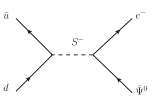
Figure 10: Feynman diagram for the parton-level process $\bar{u}d\to e^{-}\bar{\Psi}^{0}$ in SS-1.

Searches for the right-handed $W$ boson and heavy neutrino at the 13 TeV LHC with the integrated luminosities of $36.1\leavevmode\nobreak\ \text{fb}^{-1}$ ATLAS:2018dcj and $35.9\leavevmode\nobreak\ \text{fb}^{-1}$ CMS:2018agk have been performed by the ATLAS and CMS Collaborations, respectively. The ATLAS analysis ATLAS:2018dcj is divided into the same-sign and opposite-sign channels with $e^{\pm}e^{\pm}$ and $e^{+}e^{-}$, respectively. In comparison with the SSDL search, the opposite-sign dilepton search ATLAS:2018dcj suffers from much larger SM backgrounds, and is always less sensitive to the couplings $y_{e\Psi}$ and $y_{qd}$ unless the magnitudes of the couplings satisfy $|\lambda_{ed,u\Psi}|\ll|y_{e\Psi,qd}|$. In the CMS analysis CMS:2018agk there is no charge requirement on electrons, so that its sensitivity cannot compete with that of the ATLAS analysis.

Table 2: The benchmark points that we choose for the collider and $0\nu\beta\beta$-decay studies.

	$m_{\Psi}$	$m_{S}$	$m_{R}$	$\sigma_{S^{\pm}}$
BP1	$1.0\leavevmode\nobreak\ \text{TeV}$	$2.0\leavevmode\nobreak\ \text{TeV}$	$2.0\leavevmode\nobreak\ \text{TeV}$	$3.2y_{qd}^{2}\leavevmode\nobreak\ \text{pb}$
BP2	$1.9\leavevmode\nobreak\ \text{TeV}$	$2.0\leavevmode\nobreak\ \text{TeV}$	$2.0\leavevmode\nobreak\ \text{TeV}$	$3.2y_{qd}^{2}\leavevmode\nobreak\ \text{pb}$
BP3	$1.0\leavevmode\nobreak\ \text{TeV}$	$4.5\leavevmode\nobreak\ \text{TeV}$	$2.0\leavevmode\nobreak\ \text{TeV}$	$6.4y_{qd}^{2}\leavevmode\nobreak\ \text{fb}$
BP4	$3.0\leavevmode\nobreak\ \text{TeV}$	$3.5\leavevmode\nobreak\ \text{TeV}$	$2.0\leavevmode\nobreak\ \text{TeV}$	$78y_{qd}^{2}\leavevmode\nobreak\ \text{fb}$

In Tab. 2, we show four benchmark points for $m_{R}=2\leavevmode\nobreak\ \text{TeV}$ and different $m_{S}$ and $m_{\Psi}$ assuming $m_{S}>m_{\Psi}$ to ensure that the cross section of the SSDL signal is sizable enough. The cross section of $pp\to{R}^{+2/3}{R}^{-2/3}$ is $0.0155\leavevmode\nobreak\ \text{fb}$ at the 13 TeV LHC for the leptoquark mass $m_{R}=2\leavevmode\nobreak\ \text{TeV}$ Dorsner:2016wpm , while that of $pp\to S^{\pm}$ depends on the value of $y_{qd}$, as shown in the last column. After taking into account the decay branching ratios, we find that SS-2 and SS-3 always give negligible contributions compared to SS-1 unless the magnitudes of the couplings satisfy $|\lambda_{ed,u\Psi}|\ll|y_{e\Psi,qd}|$ or $|\lambda_{ed,u\Psi}|\sim|y_{e\Psi,qd}|\ll 1$.

If $|\lambda_{ed,u\Psi}|\ll|y_{e\Psi,qd}|$, the branching ratio of the lepton number violating decay $\bar{\Psi}^{0}\to e^{-}\bar{d}u$ is proportional to $\lambda^{4}/y^{4}\ll 1$, where $\lambda\sim\lambda_{ed,u\Psi}$ and $y\sim y_{qd,e\Psi}$ (for more details, the reader is referred to Appendix C), so that the cross sections of SS-1 and SS-3 are suppressed by the decay branching ratios compared to SS-2. If $|\lambda_{ed,u\Psi}|\sim|y_{e\Psi,qd}|\ll 1$, the cross section of SS-1 is suppressed by small $|y_{qd}|^{2}$, while those of SS-2 and SS-3 are not suppressed. In either case, the contribution of SS-2 and SS-3 to the SSDL signal can be comparable to that of SS-1. Nevertheless, in these two limits the sensitivity of the SSDL signal is very suppressed due to the small signal cross section, and we have checked that for the benchmark points in Tab. 2 there is no interplay of the SSDL search and $0\nu\beta\beta$ decay . Thus, we will only consider SS-1 and recast the SSDL search by the ATLAS Collaboration ATLAS:2018dcj .

The following selection criteria (SR-ee cuts) are applied in Ref. ATLAS:2018dcj . A pair of same-sign electrons with the transverse momenta $p_{T}>30\leavevmode\nobreak\ \text{GeV}$ and the pseudo-rapidity $|\eta|<2.47$ are selected. All selected events contain at least two jets with $p_{T}>100\leavevmode\nobreak\ \text{GeV}$ and $|\eta|<2.0$. The invariant masses of two electrons $(m_{ee})$ and two jets $(m_{jj})$ satisfy $m_{ee}>400\leavevmode\nobreak\ \text{GeV}$ and $m_{jj}>110\leavevmode\nobreak\ \text{GeV}$. The scalar sum of $p_{T}$ of electrons and the two most energetic jets $(H_{T})$ is larger than $400\leavevmode\nobreak\ \text{GeV}$.

In the recast, we simulate the signal process SS-1 and obtain the selection efficiencies passing the SR-ee cuts. Owing to the same selection criteria, the SM backgrounds are the same as those modelled in Ref. ATLAS:2018dcj . Thus we can easily take the number of SM background events from Ref. ATLAS:2018dcj for the integrated luminosity of $36.1\leavevmode\nobreak\ \text{fb}^{-1}$, which is $11.2$ with the SR-ee cuts being imposed. For a larger integrated luminosity $\mathcal{L}$, the number of SM background events is assumed to scale with the integrated luminosity, that is $11.2\times\mathcal{L}/(36.1\leavevmode\nobreak\ \text{fb}^{-1})$.

We use MadGraph5_aMC@NLO Alwall:2014hca to generate signal events with the PDF set NNPDF3.0NLO NNPDF:2014otw , which are passed to Pythia8 Sjostrand:2014zea and Delphes3 deFavereau:2013fsa for parton shower and detector simulation. The selection efficiencies of signals events in SS-1 passing SR-ee cuts are 0.30, 0.10, 0.27 and 0.38 for the benchmark points BP1, BP2, BP3 and BP4, respectively . Note that the selection efficiency for BP2 is smaller than those for the other benchmark points, since the energy of electron produced in association with $\Psi$ is limited by the mass difference between $m_{S}$ and $m_{\Psi}$.

After imposing SR-ee cuts, a likelihood fit of the $H_{T}$ distribution was performed in Ref. ATLAS:2018dcj to derive the observed limits, since signals tend to have larger $H_{T}$ compared to the SM backgrounds. We generate $H_{T}$ distributions of the signal SS-1 for four benchmark points, which are compared with the SM background $H_{T}$ distribution in Ref. ATLAS:2018dcj , and find that the cut $H_{T}>1.25\leavevmode\nobreak\ \text{TeV}$ can efficiently separate the signals from the SM backgrounds. The overall selection efficiencies are $0.26$, $0.09$, 0.27 and 0.38 for BP1, BP2, BP3 and BP4, respectively – which are more-or-less the same as those for $H_{T}>400\leavevmode\nobreak\ \text{GeV}$ – and only $\sim 1$ background event remains with the integrated luminosity of $36.1\leavevmode\nobreak\ \text{fb}^{-1}$. While the sensitivity of SSDL search is improved, we will only impose the SR-ee cuts to avoid an overestimate of the sensitivity.

We evaluate the exclusion limit at 95% C.L. using the asymptotic formula Cowan:2010js

$$Z_{\text{excl}}\equiv\sqrt{2[s-b\ln{((s+b)/b})]}=1.96\;,$$ (38)

where $s$ and $b$ are the numbers of signal and background events after passing the selection cuts, respectively. Besides the expected exclusion limit, we also consider the $5\sigma$ discovery potential for the SSDL search, which is obtained with Cowan:2010js

$$Z_{\text{disc}}\equiv\sqrt{2[(s+b)\ln{((s+b)/b})-s]}=5\;.$$ (39)

As mentioned earlier, to assess future prospects at the HL-LHC, we assume that the selection cuts and efficiencies remain unchanged. The sensitivities to the couplings in Eq. (2) will be discussed in Sec. 4.

3.3 Dijet resonance search

The mass of the scalar $S$ and its couplings are constrained by the dijet resonance searches at the 13 TeV LHC with the integrated luminosities of $139\leavevmode\nobreak\ \text{fb}^{-1}$ ATLAS:2019fgd and $137\leavevmode\nobreak\ \text{fb}^{-1}$ CMS:2019gwf by the ATLAS and CMS Collaborations, respectively. In both searches, the upper limits on product of signal cross section and acceptance, the latter of which depends on the transverse momenta and pseudo-rapidities of jets, for resonances in some benchmark models were obtained. A simple scaling was used in Ref. Bordone:2021cca to reinterpret the results ATLAS:2019fgd ; CMS:2019gwf in the benchmark of new gauge boson $W^{\prime}$ to other mediators. We have verified that the reinterpretation in Ref. Bordone:2021cca works well for Ref. CMS:2019gwf by the CMS Collaboration. Specifically, we generate the signal $pp\to S^{\pm}$, and assume that $S^{\pm}$ only decays into $u\bar{d}$ or $d\bar{u}$, and set $\sigma(pp\to S^{\pm})\times A$ to be equal to the limits observed by the CMS Collaboration given in Ref. CMS:2019gwf , in which the acceptance of $A=0.5$ for a scalar is declared. The upper limit on the coupling of $S^{\pm}$ to the quarks we obtain agrees well with that in Ref. Bordone:2021cca . However, the acceptance for a scalar was not reported by the ATLAS Collaboration in Ref. ATLAS:2019fgd . Using the reinterpretation results given in Ref. Bordone:2021cca , we find that the acceptance for the scalar in the ATLAS analysis ATLAS:2019fgd is about $A=0.60$, $0.89$ and $0.55$ for $m_{S}=2\leavevmode\nobreak\ \text{TeV}$, $3.5\leavevmode\nobreak\ \text{TeV}$ and $4.5\leavevmode\nobreak\ \text{TeV}$, respectively.

In Ref. ATLAS:2019fgd , the 95% C.L. observed upper limits on $\sigma_{{\rm dijet}}\times A$ are obtained after performing the likelihood fit of the dijet invariant mass distribution, where $\sigma_{{\rm dijet}}$ denotes the signal cross section. For $m_{S}=2\leavevmode\nobreak\ \text{TeV}$, $3.5\leavevmode\nobreak\ \text{TeV}$ and $4.5\leavevmode\nobreak\ \text{TeV}$, we obtain that the upper limits on $\sigma_{{\rm dijet}}$ are $38.3\leavevmode\nobreak\ \text{fb}$, $5.3\leavevmode\nobreak\ \text{fb}$ and $6.3\leavevmode\nobreak\ \text{fb}$, respectively.The projection of the upper limits are derived using Eq. (38) assuming that the numbers of signal and background events both scale with the integrated luminosity.

The total dijet cross section is given by

$$\sigma_{{\rm dijet}} =\sigma_{S^{+}}\text{Br}(S^{+}\to\bar{d}u)+\sigma_{S^{-}}\text{Br}(S^{-}\to\bar{u}d)+\sigma_{S^{0}}\text{Br}(S^{0}\to\bar{d}d)\;$$ (40)

within our signal model, where the contribution of the neutral scalar $S^{0}$ is also included. Here $\sigma_{S^{\pm}}$ and $\sigma_{S^{0}}$ are the production cross sections of $S^{\pm}$ and $S^{0}$, respectively, and “Br” denotes the decay branching ratio. By requiring the dijet cross section $\sigma_{{\rm dijet}}$ to be smaller than its observed upper limit for a given resonance mass ATLAS:2019fgd , we obtain the exclusion limits of the couplings $y_{qd}$ and $y_{e\Psi}$ at 95% C.L., which will be presented in Sec. 4.

4 Results and discussion

In Sec. 2 and Sec. 3, we have investigated the $0\nu\beta\beta$ decay and LHC searches in our simplified model, respectively. Our interest is the regime where both sets of searches provide complementary and/or overlapping sensitivities. Thus, we consider new particle masses that allow for potentially observable effects at the LHC. Specifically, we assume that the masses $m_{S}>m_{\Psi}$ and $m_{R}=2\leavevmode\nobreak\ \text{TeV}$, with benchmark values of $m_{\Psi}$ and $m_{S}$ shown in Tab. 2. From the expected sensitivity to $0\nu\beta\beta$-decay rate at future ton-scale experiments, $|y_{e\Psi}y_{qd}\lambda_{ed}\lambda_{u\Psi}|\gtrsim\mathcal{O}(10^{-3})$ is required with a sizable uncertainty due to unknown values of LECs for vector operators. For illustration, we assume the LECs $g_{V}^{\pi N}=\tilde{g}_{V}^{\pi N}=1$ and $g^{NN}_{6}=g^{NN}_{7}=0$, and the couplings $|\lambda_{ed}\lambda_{u\Psi}|=1$. For a larger (smaller) $|\lambda_{ed}\lambda_{u\Psi}|$, the sensitivity of $0\nu\beta\beta$ decay to the couplings $y_{qd}$ and $y_{e\Psi}$ is stronger (weaker), while the LHC sensitivities are less affected . Besides, the sensitivity of $0\nu\beta\beta$ decay becomes stronger (weaker) for negative (positive) values of $g^{NN}_{6,7}$. In order to differentiate the couplings $\lambda_{ed}$ and $\lambda_{u\Psi}$, a more detailed analysis of leptoquark searches in our simplified model is needed. As discussed in Sec. 3, the single production, single resonant production of the leptoquark and the Drell-Yan production are sensitive to the coupling $\lambda_{ed}$.

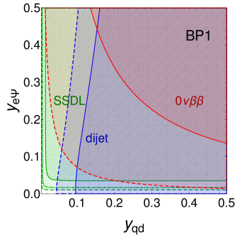
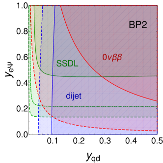
Figure 11: The current and projected sensitivities in the plane of $y_{qd}-y_{e\Psi}$ for BP1 and BP2. The red regions are excluded at 90% C.L. by the KamLAND-Zen (solid curve) and ton-scale (dashed curve) experiments. The blue regions are excluded at 95% C.L. by the dijet searches with the integrated luminosities of $139\leavevmode\nobreak\ \text{fb}^{-1}$ (solid curve) and $3\leavevmode\nobreak\ \text{ab}^{-1}$ (dashed curve). The green regions are excluded at 95% C.L. by the SSDL searches with the integrated luminosities of $36.1\leavevmode\nobreak\ \text{fb}^{-1}$ (solid curve) and $3\leavevmode\nobreak\ \text{ab}^{-1}$ (dashed curve). The green dot-dashed curves correspond to the $5\sigma$ discovery potential at the HL-LHC. The product of leptoquark couplings $|\lambda_{ed}\lambda_{u\Psi}|=1$ is assumed. $y_{e\Psi}$ and $y_{qd}$ denote the magnitudes of the couplings with the absolute value symbols omitted.

We show the sensitivities in the $0\nu\beta\beta$ decay, SSDL search and dijet search in Fig. 11 and Fig. 12. The current and projected exclusion limits are depicted in solid and dashed curves, respectively. The red regions are excluded by the $0\nu\beta\beta$-decay experiment KamLAND-Zen and future ton-scale experiments at 90% C.L. The current constraints from the SSDL search (green) and dijet search (blue) are obtained with the integrated luminosities of $36.1\leavevmode\nobreak\ \text{fb}^{-1}$ and $139\leavevmode\nobreak\ \text{fb}^{-1}$ at the 13 TeV LHC, respectively, while the future projections for the HL-LHC are made with the integrated luminosity of $3\leavevmode\nobreak\ \text{ab}^{-1}$. We also show the $5\sigma$ discovery potential of the SSDL search at the HL-LHC in green dot-dashed curve.

Both the SSDL and dijet searches are sensitive to the scalar mass $m_{S}$. For relatively small $m_{S}$, the cross section of $pp\to S^{\pm}$ is sizable for BP1 and BP2. From the left panel of Fig. 11, the accessible region of $y_{qd}$ and $y_{e\Psi}$ (the absolute value symbols are omitted) at future ton-scale $0\nu\beta\beta$-experiments has already been excluded by the existing SSDL and dijet searches for BP1. In such a scenario, there is no signal expected in $0\nu\beta\beta$-decay experiments barring extremely small $y_{qd}$.

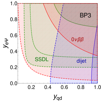
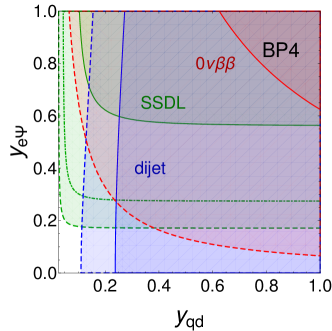
Figure 12: Same as Fig. 11 but for BP3 and BP4.

The $0\nu\beta\beta$-decay and LHC experiments are complementary for the other benchmark points. For BP2, $m_{\Psi}$ is close to $m_{S}$, so that the decay branching ratio of $S^{\pm}\to e^{\pm}\Psi$ is largely suppressed and the selection efficiency in the SSDL search is smaller compared to BP1. In the right panel of Fig. 11, we can see that the combination of the existing SSDL and dijet searches gives stronger constraints compared to the $0\nu\beta\beta$-decay search at KamLAND-Zen. For $y_{qd}\lesssim 0.1$, which is currently allowed, it is possible to observe a TeV-scale LNV signal in a large portion of the region $y_{e\Psi}\gtrsim 0.25$ in both future $0\nu\beta\beta$-decay and SSDL searches. If however no signal is observed, most of the region $y_{e\Psi}\gtrsim 0.15$ can be excluded.

In Fig. 12, larger values of $m_{S}$ are considered. The cross sections of $pp\to S^{\pm}$ for BP3 and BP4 are smaller than those for BP1 and BP2 by $2-3$ orders of magnitude, as seen in Tab. 2. For BP3, the sensitivities to the couplings $y_{qd}$ and $y_{e\Psi}$ in KamLAND-Zen and future ton-scale $0\nu\beta\beta$-decay experiments are always better than those of the current and projected SSDL searches, respectively, which is shown in the left panel. In addition, the constraint from the existing dijet search is much weaker than that for BP1 and BP2. For future prospects, the dijet search can probe a large portion of the region $y_{qd}\gtrsim 0.4$. One can observe TeV-scale LNV signal in both future SSDL and $0\nu\beta\beta$-decay searches for $y_{e\Psi}\gtrsim 0.35$ and $y_{qd}\gtrsim 0.15$, which is indicated by the $5\sigma$ contour. If signal of LNV is only observed in ton-scale $0\nu\beta\beta$-decay experiments, it implies that either $y_{e\Psi}\lesssim 0.2$ or $y_{qd}\lesssim 0.1$, which could be distinguished using the dijet searches.

For BP1, BP2 and BP3, we have assumed that the Dirac fermion mass $m_{\Psi}$ is below the leptoquark mass $m_{R}$. For BP4, an alternative scenario $m_{\Psi}>m_{R}$ is considered, and $m_{S}$ is slightly larger than $m_{\Psi}$. In comparison with BP1, the sensitivity of SSDL search is reduced due to the smaller production cross section and decay branching ratio of $S^{\pm}$, although the decay branching ratio of $\Psi$ increases. Besides, the sensitivity of $0\nu\beta\beta$ decay also degrades, since the decay rate is proportional to $1/(m_{S}^{4}m_{R}^{4}m_{\Psi}^{2})$. In the right panel of Fig. 12, we can see that the projected sensitivity of SSDL search at the HL-LHC is better than that of $0\nu\beta\beta$ decay in ton-scale experiments in contrast to BP3, after taking into account the constraint from the dijet search. In analogy with BP2, it is very promising to observe TeV-scale LNV for $y_{e\Psi}\gtrsim 0.3$. We also note that BP2 and BP4 might be distinguished with differential distributions, such as $p_{T}$ of electron or jets and $H_{T}$.

It is worth noting a few caveats about our projections: if the mass of the new particles is sufficiently large, the LHC loses sensitivity and a future $pp$ collider may be needed; we assumed the same set of selection cuts and efficiencies that occurs, at the time of this writing, in LHC collaboration analyses of 13 TeV LHC data; and we did not include any effects due to pile-up or pile-up subtraction. Our results indicate that the HL-LHC has promising prospects for uncovering the chirally-suppressed mechanism with TeV-scale LNV, that is complementary to the on-going $0\nu\beta\beta$ decay experiments. Our results suggest a more detailed study including more realistic assessment of backgrounds and optimizing the reach of the HL-LHC for TeV-scale LNV is warranted.

5 Conclusion

In this work, we have studied $\Delta L=2$ LNV interactions, whose contributions to $0\nu\beta\beta$ decay are chirally suppressed in a simplified model. While the $0\nu\beta\beta$ decay is insensitive to the details of underlying mechanism, the LHC can provide complementary tests in the same-sign dilepton plus dijet search channel and, by using dijet and leptoquark searches, further distinguish different scenarios of TeV-scale LNV in our simplified model. We have calculated the half-life of $0\nu\beta\beta$ decay, and investigated the current and projected sensitivities of the LHC searches.

In three of the benchmark points we examined (BP1, BP2, and BP4), we find that due to the on-shell production of a $2-3.5$ TeV charged scalar $(S^{\pm})$ in the $s$-channel at the LHC, the sensitivities of SSDL searches are better than those of $0\nu\beta\beta$-decay searches. Dijet searches can place severe constraints, and in particular a large portion of parameter space accessible to future SSDL and $0\nu\beta\beta$-decay searches has been excluded by the existing dijet search. However, for a fourth benchmark point (BP3) in which the scalar particle has a mass of 4.5 TeV, we find that $0\nu\beta\beta$-decay searches have a better sensitivity compared to the SSDL search, and the constraint from dijet search is much weaker. In all of the scenarios that we consider, most of the region within reach of the $0\nu\beta\beta$-decay search at future ton-scale $0\nu\beta\beta$-decay experiments can be covered at the $5\sigma$ discovery level in the SSDL search at the HL-LHC.

From the benchmark studies, we could obtain some general results about the future $0\nu\beta\beta$-decay and LHC searches for TeV-scale LNV, which at low energies generates dimension-9 vector operators:

• If one observes a LNV signal in the SSDL search but not in $0\nu\beta\beta$ decay, it implies that either the coupling of scalar to quark or lepton is extremely small (e.g. BP1) or the masses of new Dirac fermion and scalar are close (e.g. BP2 and BP4).

• If one observes a LNV signal in $0\nu\beta\beta$ decay but not in the SSDL search, however, there might exist a heavy scalar with its coupling to quarks or leptons is small (e.g. BP3).

• If LNV signals are observed in both $0\nu\beta\beta$ decay and SSDL search, either the production or decay of the scalar at the LHC is suppressed (e.g. BP2, BP3 and BP4).

• If there is no LNV signal observed, then LNV may have other origins or lepton number may be conserved at the classical (Lagrangian) level.

In case of LNV signal(s) being observed, depending on whether we observe a signal in dijet search, we know that the coupling of scalar to quarks is large or not.

In this work we have focused on the potential of the LHC to search for the particles and interactions in the simplified model underlie the dimension-9 LNV operators. It would be interesting to extend our analysis of LHC searches. It would also be interesting to revisit the issues explored here in a model that has acceptable levels of flavor-changing neutral current and charged lepton number violating processes.

Appendix A Hadron-level $0\nu\beta\beta$-decay amplitudes: comparing dimension-9 LNV vector and scalar operators

Below the GeV scale, dimension-9 LNV quark-lepton operators induce local LNV hadron-lepton interactions. These can be described using chiral pertubration theory, which is an effective theory with an expansion parameter $\epsilon_{\chi}\equiv q/\Lambda_{\chi}$. Here $\Lambda_{\chi}\simeq 1$ GeV and $q$ is a typical momentum-transfer scale of the nuclear $0\nu\beta\beta$ decay $0^{+}\rightarrow 0^{+}$, with $q\simeq m_{\pi}$. For dimension-9 LNV operators, their leading interactions with hadrons are through induced local $\pi\pi ee$, $\pi NNee$ and $NNNNee$ operators. For the sake of brevity, we will not give the explicit forms of the dimension-9 LNV operators. For further details the reader is referred to Ref. Cirigliano:2018yza .

For all dimension-9 vector operators $O^{\mu}_{6,7,8,9}$ and $O^{\mu\prime}_{6,7,8,9}$, no sizable non-derivative $\pi\pi ee$ operators are generated at LO Prezeau:2003xn or through N²LO Graesser:2016bpz . The LNV operators induced by the vector operators that involve two $\pi$’s are of the form $(\pi\partial^{\mu}\pi)\overline{e}\gamma^{\mu}\gamma_{5}e^{c}$, and $(\partial^{\nu}\pi)(\partial_{\nu}\partial^{\mu}\pi)\overline{e}\gamma^{\mu}\gamma_{5}e^{c}$, at LO and N²LO respectively. The point here is that the pion equations of motion can be used to show that all of these local operators are proportional to the non-derivative operator $\pi\pi ee$ with a coefficient proportional to the electron mass $m_{e}$ and therefore negligible at this level.

In the Weinberg power counting therefore, the leading contributions of vector operators to the amplitude arise from $\pi NNee$ and $NNNNee$ operators which both contribute at $\mathcal{O}(\epsilon^{2}_{\chi})$ to the $nn\rightarrow ppee$ amplitude.

Naïvely then, the transition amplitude arising from dimension-9 vector operators is suppressed by $\mathcal{O}(\epsilon^{2}_{\chi})$ compared to that of scalar operators that arise from $O_{2,3,4,5}$ and $O^{\prime}_{2,3}$ which contribute at $\mathcal{O}(\epsilon^{0}_{\chi})$ to the amplitude. While we find this expectation to generally be true, it depends on an interplay between NMEs and the size of unknown LECs that occurs, in the case of scalar operators, in the expression for the amplitude. The point of this Appendix is to expand on this statement.

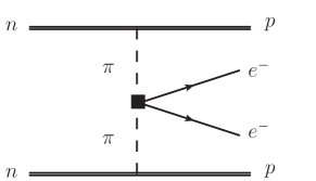
Figure 13: For scalar operators, the amplitude for $nn\rightarrow ppee$ receives an additional contribution from the Feynman diagram shown here, which must be combined with those shown in Fig. 2.

Going into further detail, the reason dimension-9 scalar operators $O_{2,3,4,5}$ and $O^{\prime}_{2,3}$ contribute at $\mathcal{O}(\epsilon^{0}_{\chi})$ to the amplitude is because they induce non-derivative $\pi\pi ee$ operators that are unsuppressed by $m_{e}$ or any chiral power. In this case the total amplitude is given by summing the Feynman diagrams in Fig. 13, together with Fig. 2. For these scalar operators, in the Weinberg power counting, the second diagram in Fig. 2 is naïvely suppressed to the diagram in Fig. 13 by $\epsilon^{2}_{\chi}$. But there is a further subtlety: the contribution of the local $\pi\pi ee$ operator to the total amplitude, obtained by solving the Lippman-Schwinger equation for the strong $NN$ potential, is actually UV divergent. Requiring that the total amplitude is independent of the regulator necessitates promoting the local $NNNNee$ operator from N²LO to LO, which would violate Weinberg’s power counting. The RG equation relating the LECs of the $\pi\pi ee$ and $NNNNee$ operators suggests that the LEC of the latter is actually larger by a factor of $(4\pi)^{2}$ compared to NDA. So that in the chiral power counting, the diagram in Fig. 13 and the second diagram in Fig. 2 contribute at the same order Cirigliano:2018hja ; Cirigliano:2018yza ; Cirigliano:2019vdj . This feature will be important to the discussion that follows.

To see this explicitly, the contributions of dimension-9 scalar operators to the amplitude for nuclear $0\nu\beta\beta$ decay $0^{+}\to 0^{+}$ is given by Cirigliano:2018yza

$$\mathcal{A}_{\text{scalar}}=\dfrac{g_{A}^{2}G_{F}^{2}m_{e}}{\pi R_{A}}\left[\mathcal{A}_{\nu}\bar{u}(k_{1})P_{R}C\bar{u}^{T}(k_{2})+\mathcal{A}_{R}\bar{u}(k_{1})P_{L}C\bar{u}^{T}(k_{2})\right]\;,$$ (41)

where the reduced amplitudes $\mathcal{A}_{\nu}$ and $\mathcal{A}_{R}$ are

$$\mathcal{A}_{\nu}(\mathcal{A}_{R}) = \frac{m^{2}_{N}}{m_{e}v}\left[-\frac{1}{2m^{2}_{N}}C^{(9)}_{\pi\pi L(R)}M_{PS,sd}+\frac{m^{2}_{\pi}}{2m^{2}_{N}}C^{(9)}_{\pi NL(R)}M_{P,sd}-\frac{2}{g^{2}_{A}}\frac{m^{2}_{\pi}}{m^{2}_{N}}C^{(9)}_{NNL(R)}M_{F,sd}\right]$$ (42)

where $C^{(9)}_{\pi\pi L(R)}$, $C^{(9)}_{\pi NL(R)}$, and $C^{(9)}_{NNL(R)}$ are linear in the Wilson coefficients $C_{i}$ of the dimension-9 scalar operators, and in LECs. Their detailed expressions do not matter for this discussion, but can be found in Ref. Cirigliano:2018yza . Each of these is multiplied by the NMEs

$$M_{PS,sd} \equiv \frac{1}{2}M^{AP}_{GT,sd}+M^{PP}_{GT,sd}+\frac{1}{2}M^{AP}_{T,sd}+M^{PP}_{T,sd},$$ (43)

$$M_{P,sd} \equiv M^{AP}_{GT,sd}+M^{AP}_{T,sd}\leavevmode\nobreak\ ,$$ (44)

which are linear combination of short distance Gamow-Teller and tensor nuclear matrix elements, and by a short-distance Fermi nuclear matrix element $M_{F,sd}$, respectively. Expressions for these matrix elements in terms of “neutrino potentials” can also be found in Ref. Cirigliano:2018yza .

Next, first consider the value of $M_{PS,sd}$. For ¹³⁶Xe, $M_{GT,sd}^{AP}=-2.80$, $M_{GT,sd}^{PP}=1.06$, $M_{T,sd}^{AP}=-0.92$ and $M^{PP}_{T,sd}=0.36$, calculated using the quasi-particle random phase approximation (QRPA) Hyvarinen:2015bda . While the first three NMEs are $\mathcal{O}(1)$, a partial cancellation occurs in the summation: $M_{PS,sd}=-0.44$. A similar pattern of partial cancellation across other isotopes ⁷⁶Ge, ⁸²Se, and ¹³⁰Te, whether evaluated by QRPA Hyvarinen:2015bda , shell models Menendez:2017fdf , or interacting boson models (IBM) Barea:2015kwa ; Deppisch:2020ztt is seen to occur:

$$M_{PS,sd}$$ ⁷⁶Ge ⁸²Se ¹³⁰Te ¹³⁶Xe

QRPA Hyvarinen:2015bda

Shell Menendez:2017fdf

IBM  Barea:2015kwa

(45)

For vector operators, the NME for the left diagram appearing in Fig. 2 is given by $M_{P,sd}$, and is currently

$$M_{P,sd}$$ ⁷⁶Ge ⁸²Se ¹³⁰Te ¹³⁶Xe

QRPA Hyvarinen:2015bda

Shell Menendez:2017fdf

IBM  Barea:2015kwa

(46)

Let’s now consider each of the three terms in Eq. (42) in turn. The first one arises from induced $\pi\pi ee$ interactions. Specifically, $C^{(9)}_{\pi\pi L(R)}$ depends on the Wilson coefficients $C_{i}$ and the LECs $g^{\pi\pi}_{i=2,3,4,5}$, the latter of which are known from chiral $SU(3)$ Cirigliano:2017ymo and lattice QCD Nicholson:2018mwc to be $\sim$ few $\times$ GeV², in agreement with naïve dimensional analysis (NDA). Thus all else being equal, the size of the quantity $C^{(9)}_{\pi\pi L(R)}/m^{2}_{N}$ is just given by the size of the Wilson coefficients $C_{i}$ appearing in the expressions for $C^{(9)}_{\pi\pi L(R)}$.

For the second term, $C^{(9)}_{\pi NL(R)}$ depends on $g^{\pi N}_{1}$ and $g^{\pi\pi}_{1}$, which at this chiral order only occurs for $O_{1}$ and $O^{\prime}_{1}$. Since we are not considering $O_{1}$ and $O^{\prime}_{1}$ in this Appendix, we can neglect the second term in our comparison of the scalar operators $O_{2,3,4,5}$ and $O^{\prime}_{2,3}$ to the vector operators.

The last term in Eq. (42) arises from induced 4-nucleon operators ($NNNNee$), and is from the diagram on the right in Fig. 2. It is naïvely suppressed compared to the first term, depending as it does on the explicit factor of $m^{2}_{\pi}/m^{2}_{N}$. However, the prefactor $C^{(9)}_{NNL(R)}$ depends on the LECs $g^{NN}_{i}$, and RG evolution suggests $g^{NN}_{2,3,4,5}=\mathcal{O}((4\pi)^{2})$ Cirigliano:2018yza ; Cirigliano:2019vdj . If these LECs are that large then the last term cannot be neglected.

But first suppose these LECs are much smaller than $\mathcal{O}((4\pi)^{2})$. Then the ratio of amplitudes induced by vector operators to scalar operators is, all else being equal,

$$\frac{\mathcal{A}_{\text{vector}}}{\mathcal{A}_{\text{scalar}}}\simeq\frac{m^{2}_{\pi}}{m^{2}_{N}}\frac{M_{P,sd}}{M_{PS,sd}}\leavevmode\nobreak\ .$$ (47)

The ratio of NMEs appearing above is currently

$$M_{P,sd}/M_{PS,sd}$$ ⁷⁶Ge ⁸²Se ¹³⁰Te ¹³⁶Xe

QRPA

Shell

IBM

(48)

and exhibits remarkable stability across isotopes and methods for estimating the NMEs. In particular, this ratio is $\mathcal{O}(6-8)$, and is driven by the “small” values of the NME appearing in $\mathcal{A}_{\text{scalar}}$, rather than a suppression of the NME appearing in $\mathcal{A}_{\text{vector}}$.

In other words, under the assumption that the contribution of the right diagram in Fig. 2 to $\mathcal{A}_{\text{scalar}}$ is $\mathcal{O}(m^{2}_{\pi}/m_{N}^{2})\simeq 1/60$, the amplitude $\mathcal{A}_{\text{vector}}$ is only suppressed compared to $\mathcal{A}_{\text{scalar}}$ by an amount $\simeq(6-8)/60$, rather than $1/60.$

This conclusion is however sensitive to the unknown values of the LECs $g^{NN}_{i}$ contributing to $\mathcal{A}_{\text{scalar}}$, as we now explain. The reason is that in the expression for $\mathcal{A}_{\text{scalar}}$, the contribution of the 4-nucleon operator is weighted by the NME $M_{F,sd}$, which are not small:

$$M_{F,sd}$$ ⁷⁶Ge ⁸²Se ¹³⁰Te ¹³⁶Xe

QRPA Hyvarinen:2015bda

Shell Menendez:2017fdf

IBM  Barea:2015kwa

(49)

In the extreme situation that the LECs $g^{NN}_{2,3,4,5}\simeq\mathcal{O}((4\pi)^{2})$, the relevant comparison of NME’s is instead to $M_{P,sd}/M_{F,sd}$

$$M_{P,sd}/M_{F,sd}$$ ⁷⁶Ge ⁸²Se ¹³⁰Te ¹³⁶Xe

QRPA Hyvarinen:2015bda

Shell Menendez:2017fdf

IBM  Barea:2015kwa

(50)

which varies on the $\mathcal{O}(1.5-2.5)$.

Of course, the enhancement of the LECs appearing in the $0\nu\beta\beta$-decay amplitude induced by the scalar operators $O_{2,3,4,5}$ and $O^{\prime}_{2,3}$ may not be as large as $(4\pi)^{2}$. In that case the comparison between the $0\nu\beta\beta$-decay amplitude induced by vector and scalar operators lies somewhere between the two extremes described here. Reducing the uncertainty on the sizes of the LECs is greatly needed.

Appendix B Neutrino mass

In the full theory where all the fields are not integrated out, a neutrino mass is first generated at three-loop order, as shown, for example, by the Feynman diagram given in Fig. 14. If $S$ acquires a vev $\langle S\rangle$, then a neutrino mass is generated at two-loop order, as can be seen from a straightforward inspection of Fig. 14. In either case, the estimate size of the neutrino mass from these effects is far below the actual value of neutrino masses, as discussed in Sec. 2.

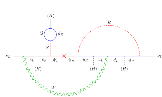
Figure 14: An illustrative LNV Feynman diagram of the UV theory that contributes to the neutrino mass. The heavy degrees of freedom are highlighted in red.

Appendix C Partial decay widths

In this appendix, we provide the decay widths of the new particles in our simplified model. For brevity, all of the couplings are assumed to be real and the step functions $\theta(m_{X}-m_{Y})$ for the decay processes $X\to Y+\dots$ are omitted.

The two-body decay widths of $\Psi^{0}$ and $S^{+}$ are

$$\Gamma(S^{+}\to\Psi^{0}e^{+}) =\dfrac{y_{e\Psi}^{2}(m_{S}^{2}-m_{\Psi}^{2})^{2}}{16\pi m_{S}^{3}}\;,$$ (51)

$$\Gamma(\Psi^{0}\to S^{+}e^{-}) =\dfrac{y_{e\Psi}^{2}(m_{\Psi}^{2}-m_{S}^{2})^{2}}{32\pi m_{\Psi}^{3}}\;,$$ (52)

$$\Gamma(S^{+}\to\bar{d}u) =\dfrac{3}{16\pi}m_{S}(y_{qu}^{2}+y_{qd}^{2})\;,$$ (53)

$$\Gamma(\Psi^{0}\to{R}^{2/3}\bar{u}) =\Gamma(\Psi^{-}\to{R}^{-1/3}\bar{u})$$

$$=\dfrac{\lambda_{u\Psi}^{2}(m_{\Psi}^{2}-m_{R}^{2})^{2}}{16\pi m_{R}^{3}}\;.$$ (54)

The two-body decay widths of $\Psi^{-}$ and $S^{0}$ are

$$\Gamma(S^{0}\to\bar{d}d) =\dfrac{3}{16\pi}m_{S}y_{qd}^{2}\;,$$ (55)

$$\Gamma(S^{0}\to\bar{u}u) =\dfrac{3}{16\pi}m_{S}y_{qu}^{2}\;,$$ (56)

$$\Gamma(\Psi^{-}\to S^{0}e^{-}) =\dfrac{y_{e\Psi}^{2}(m_{\Psi}^{2}-m_{S}^{2})^{2}}{64\pi m_{\Psi}^{3}}\;,$$ (57)

$$\Gamma(S^{0}\to\Psi^{+}e^{-}) =\dfrac{y_{e\Psi}^{2}(m_{S}^{2}-m_{\Psi}^{2})^{2}}{32\pi m_{S}^{3}}\;,$$ (58)

$$\Gamma(S^{0}\to\Psi^{-}e^{+}) =\dfrac{y_{e\Psi}^{2}(m_{S}^{2}-m_{\Psi}^{2})^{2}}{32\pi m_{S}^{3}}\;.$$ (59)

The two-body decay widths of ${R}$ are

$$\Gamma({R}^{2/3}\to e^{+}d) =\Gamma({R}^{-1/3}\to\bar{\nu}d)$$

$$=\dfrac{\lambda_{ed}^{2}m_{R}}{16\pi}\;,$$ (60)

$$\Gamma({R}^{2/3}\to\Psi^{0}u) =\Gamma({R}^{-1/3}\to\Psi^{-}u)$$

$$=\dfrac{\lambda_{u\Psi}^{2}(m_{R}^{2}-m_{\Psi}^{2})^{2}}{16\pi m_{R}^{3}}\;.$$ (61)

For the three-body decay widths of $\Psi^{0}$ are computed numerically using MadGraph5_aMC@NLO Alwall:2014hca and checked with CalcHEP Belyaev:2012qa . For the sake of convenience, we provide the decay widths in the limit of $m_{\Psi}\ll m_{S}$, $m_{R}$

$$\Gamma(\Psi^{0}\to e^{-}u\bar{d}) =\dfrac{1}{2048\pi^{3}}\dfrac{m_{\Psi}^{5}}{m_{S}^{4}}y_{e\Psi}^{2}(y_{qu}^{2}+y_{qd}^{2})\;,$$ (62)

$$\Gamma(\Psi^{0}\to e^{+}\bar{u}d) =\dfrac{1}{2048\pi^{3}}\dfrac{m_{\Psi}^{5}}{m_{R}^{4}}\lambda_{ed}^{2}\lambda_{u\Psi}^{2}\;.$$ (63)

Because the lepton number of $\Psi^{0}$ is $+1$, the decay $\Psi^{0}\to e^{-}u\bar{d}$ conserves lepton number whereas $\Psi^{0}\to e^{+}\bar{u}d$ violates it.

References

- (1) P. Minkowski, at a Rate of One Out of Muon Decays?, Phys. Lett. B 67 (1977) 421–428.
- (2) M. Gell-Mann, P. Ramond and R. Slansky, Complex Spinors and Unified Theories, Conf. Proc. C 790927 (1979) 315–321, [1306.4669].
- (3) S. L. Glashow, The Future of Elementary Particle Physics, NATO Sci. Ser. B 61 (1980) 687.
- (4) T. Yanagida, Horizontal Symmetry and Masses of Neutrinos, Prog. Theor. Phys. 64 (1980) 1103.
- (5) R. N. Mohapatra and G. Senjanovic, Neutrino Mass and Spontaneous Parity Nonconservation, Phys. Rev. Lett. 44 (1980) 912.
- (6) J. Schechter and J. W. F. Valle, Neutrino Masses in SU(2) x U(1) Theories, Phys. Rev. D 22 (1980) 2227.
- (7) A. Abada, C. Biggio, F. Bonnet, M. B. Gavela and T. Hambye, Low energy effects of neutrino masses, JHEP 12 (2007) 061, [0707.4058].
- (8) P. W. Angel, N. L. Rodd and R. R. Volkas, Origin of neutrino masses at the LHC: effective operators and their ultraviolet completions, Phys. Rev. D 87 (2013) 073007, [1212.6111].
- (9) A. Pilaftsis and T. E. J. Underwood, Resonant leptogenesis, Nucl. Phys. B 692 (2004) 303–345, [hep-ph/0309342].
- (10) F. F. Deppisch, L. Graf, J. Harz and W.-C. Huang, Neutrinoless Double Beta Decay and the Baryon Asymmetry of the Universe, Phys. Rev. D 98 (2018) 055029, [1711.10432].
- (11) J. Harz, M. J. Ramsey-Musolf, T. Shen and S. Urrutia-Quiroga, TeV-scale Lepton Number Violation: Connecting Leptogenesis, Neutrinoless Double Beta Decay, and Colliders, 2106.10838.
- (12) J. C. Helo, M. Hirsch, S. G. Kovalenko and H. Pas, Neutrinoless double beta decay and lepton number violation at the LHC, Phys. Rev. D 88 (2013) 011901, [1303.0899].
- (13) T. Peng, M. J. Ramsey-Musolf and P. Winslow, TeV lepton number violation: From neutrinoless double- decay to the LHC, Phys. Rev. D 93 (2016) 093002, [1508.04444].
- (14) A. De Gouvêa, W.-C. Huang, J. König and M. Sen, Accessible Lepton-Number-Violating Models and Negligible Neutrino Masses, Phys. Rev. D 100 (2019) 075033, [1907.02541].
- (15) Planck collaboration, N. Aghanim et al., Planck 2018 results. VI. Cosmological parameters, Astron. Astrophys. 641 (2020) A6, [1807.06209].
- (16) M. Hazumi et al., LiteBIRD: a small satellite for the study of B-mode polarization and inflation from cosmic background radiation detection, Proc. SPIE Int. Soc. Opt. Eng. 8442 (2012) 844219.
- (17) Euclid collaboration, R. Scaramella et al., Euclid space mission: a cosmological challenge for the next 15 years, IAU Symp. 306 (2014) 375–378, [1501.04908].
- (18) T. Brinckmann, D. C. Hooper, M. Archidiacono, J. Lesgourgues and T. Sprenger, The promising future of a robust cosmological neutrino mass measurement, JCAP 01 (2019) 059, [1808.05955].
- (19) K. Abazajian et al., CMB-S4 Science Case, Reference Design, and Project Plan, 1907.04473.
- (20) DESI collaboration, M. E. Levi et al., The Dark Energy Spectroscopic Instrument (DESI), 1907.10688.
- (21) G. Li, M. Ramsey-Musolf and J. C. Vasquez, Left-right symmetry and leading contributions to neutrinoless double beta decay, 2009.01257.
- (22) G. Prezeau, M. Ramsey-Musolf and P. Vogel, Neutrinoless double beta decay and effective field theory, Phys. Rev. D 68 (2003) 034016, [hep-ph/0303205].
- (23) A. Faessler, S. Kovalenko, F. Simkovic and J. Schwieger, Dominance of pion exchange in R-parity violating supersymmetry contributions to neutrinoless double beta decay, Phys. Rev. Lett. 78 (1997) 183–186, [hep-ph/9612357].
- (24) S. Weinberg, Nuclear forces from chiral Lagrangians, Phys. Lett. B 251 (1990) 288–292.
- (25) S. Weinberg, Effective chiral Lagrangians for nucleon - pion interactions and nuclear forces, Nucl. Phys. B 363 (1991) 3–18.
- (26) D. B. Kaplan, M. J. Savage and M. B. Wise, Nucleon - nucleon scattering from effective field theory, Nucl. Phys. B 478 (1996) 629–659, [nucl-th/9605002].
- (27) W. Rodejohann, Neutrino-less Double Beta Decay and Particle Physics, Int. J. Mod. Phys. E 20 (2011) 1833–1930, [1106.1334].
- (28) F. Bonnet, M. Hirsch, T. Ota and W. Winter, Systematic decomposition of the neutrinoless double beta decay operator, JHEP 03 (2013) 055, [1212.3045].
- (29) J. C. Helo, M. Hirsch, H. Päs and S. G. Kovalenko, Short-range mechanisms of neutrinoless double beta decay at the LHC, Phys. Rev. D 88 (2013) 073011, [1307.4849].
- (30) V. Cirigliano, W. Dekens, J. de Vries, M. L. Graesser and E. Mereghetti, A neutrinoless double beta decay master formula from effective field theory, JHEP 12 (2018) 097, [1806.02780].
- (31) V. Cirigliano, W. Dekens, J. De Vries, M. L. Graesser, E. Mereghetti, S. Pastore et al., Renormalized approach to neutrinoless double- decay, Phys. Rev. C 100 (2019) 055504, [1907.11254].
- (32) V. Cirigliano, W. Dekens, J. De Vries, M. L. Graesser, E. Mereghetti, S. Pastore et al., New Leading Contribution to Neutrinoless Double- Decay, Phys. Rev. Lett. 120 (2018) 202001, [1802.10097].
- (33) V. Cirigliano, W. Dekens, J. de Vries, M. Hoferichter and E. Mereghetti, Toward Complete Leading-Order Predictions for Neutrinoless Double Decay, Phys. Rev. Lett. 126 (2021) 172002, [2012.11602].
- (34) V. Cirigliano, W. Dekens, J. de Vries, M. Hoferichter and E. Mereghetti, Determining the leading-order contact term in neutrinoless double decay, JHEP 05 (2021) 289, [2102.03371].
- (35) DELPHES 3 collaboration, J. de Favereau, C. Delaere, P. Demin, A. Giammanco, V. Lemaître, A. Mertens et al., DELPHES 3, A modular framework for fast simulation of a generic collider experiment, JHEP 02 (2014) 057, [1307.6346].
- (36) M. L. Graesser, An electroweak basis for neutrinoless double decay, JHEP 08 (2017) 099, [1606.04549].
- (37) V. Cirigliano, W. Dekens, J. de Vries, M. L. Graesser and E. Mereghetti, Neutrinoless double beta decay in chiral effective field theory: lepton number violation at dimension seven, JHEP 12 (2017) 082, [1708.09390].
- (38) KamLAND-Zen collaboration, A. Gando et al., Search for Majorana Neutrinos near the Inverted Mass Hierarchy Region with KamLAND-Zen, Phys. Rev. Lett. 117 (2016) 082503, [1605.02889].
- (39) J. Schechter and J. W. F. Valle, Neutrinoless Double beta Decay in SU(2) x U(1) Theories, Phys. Rev. D 25 (1982) 2951.
- (40) P.-T. Chen, G.-J. Ding and C.-Y. Yao, Decomposition of short-range decay operators at one-loop level, 2110.15347.
- (41) M. B. Wise and Y. Zhang, Effective Theory and Simple Completions for Neutrino Interactions, Phys. Rev. D 90 (2014) 053005, [1404.4663].
- (42) Y. Liao and X.-D. Ma, An explicit construction of the dimension-9 operator basis in the standard model effective field theory, JHEP 11 (2020) 152, [2007.08125].
- (43) H.-L. Li, Z. Ren, M.-L. Xiao, J.-H. Yu and Y.-H. Zheng, Complete set of dimension-nine operators in the standard model effective field theory, Phys. Rev. D 104 (2021) 015025, [2007.07899].
- (44) H.-L. Li, Z. Ren, M.-L. Xiao, J.-H. Yu and Y.-H. Zheng, Low energy effective field theory operator basis at d 9, JHEP 06 (2021) 138, [2012.09188].
- (45) V. Bernard, N. Kaiser and U.-G. Meissner, Chiral dynamics in nucleons and nuclei, Int. J. Mod. Phys. E 4 (1995) 193–346, [hep-ph/9501384].
- (46) J. Gasser and H. Leutwyler, Chiral Perturbation Theory to One Loop, Annals Phys. 158 (1984) 142.
- (47) E. E. Jenkins and A. V. Manohar, Baryon chiral perturbation theory using a heavy fermion Lagrangian, Phys. Lett. B 255 (1991) 558–562.
- (48) A. Manohar and H. Georgi, Chiral Quarks and the Nonrelativistic Quark Model, Nucl. Phys. B 234 (1984) 189–212.
- (49) S. Weinberg, Larger Higgs Exchange Terms in the Neutron Electric Dipole Moment, Phys. Rev. Lett. 63 (1989) 2333.
- (50) J. Hyvärinen and J. Suhonen, Nuclear matrix elements for decays with light or heavy Majorana-neutrino exchange, Phys. Rev. C 91 (2015) 024613.
- (51) M. Horoi and A. Neacsu, Towards an effective field theory approach to the neutrinoless double-beta decay, 1706.05391.
- (52) D. Stefanik, R. Dvornicky, F. Simkovic and P. Vogel, Reexamining the light neutrino exchange mechanism of the decay with left- and right-handed leptonic and hadronic currents, Phys. Rev. C 92 (2015) 055502, [1506.07145].
- (53) M. Doi, T. Kotani and E. Takasugi, Double beta Decay and Majorana Neutrino, Prog. Theor. Phys. Suppl. 83 (1985) 1.
- (54) G. Li, M. J. Ramsey-Musolf, S. Su and J. C. Vasquez, Lepton Number Violation: from Decay to Long-Lived Particle Searches, 2109.08172.
- (55) GERDA collaboration, M. Agostini et al., Final Results of GERDA on the Search for Neutrinoless Double- Decay, Phys. Rev. Lett. 125 (2020) 252502, [2009.06079].
- (56) nEXO collaboration, S. A. Kharusi et al., nEXO Pre-Conceptual Design Report, 1805.11142.
- (57) LEGEND collaboration, N. Abgrall et al., The Large Enriched Germanium Experiment for Neutrinoless Double Beta Decay (LEGEND), AIP Conf. Proc. 1894 (2017) 020027, [1709.01980].
- (58) CUPID collaboration, W. Armstrong et al., CUPID pre-CDR, 1907.09376.
- (59) SNO+ collaboration, J. Paton, Neutrinoless Double Beta Decay in the SNO+ Experiment, in Prospects in Neutrino Physics, 3, 2019. 1904.01418.
- (60) X. Chen et al., PandaX-III: Searching for neutrinoless double beta decay with high pressure136Xe gas time projection chambers, Sci. China Phys. Mech. Astron. 60 (2017) 061011, [1610.08883].
- (61) NEXT collaboration, C. Adams et al., Sensitivity of a tonne-scale NEXT detector for neutrinoless double beta decay searches, 2005.06467.
- (62) M. Duerr, M. Lindner and A. Merle, On the Quantitative Impact of the Schechter-Valle Theorem, JHEP 06 (2011) 091, [1105.0901].
- (63) S. Pastore, J. Carlson, V. Cirigliano, W. Dekens, E. Mereghetti and R. B. Wiringa, Neutrinoless double- decay matrix elements in light nuclei, Phys. Rev. C 97 (2018) 014606, [1710.05026].
- (64) ATLAS collaboration, G. Aad et al., Search for pairs of scalar leptoquarks decaying into quarks and electrons or muons in = 13 TeV collisions with the ATLAS detector, JHEP 10 (2020) 112, [2006.05872].
- (65) CMS collaboration, V. Khachatryan et al., Search for single production of scalar leptoquarks in proton-proton collisions at , Phys. Rev. D 93 (2016) 032005, [1509.03750].
- (66) M. Schmaltz and Y.-M. Zhong, The leptoquark Hunter’s guide: large coupling, JHEP 01 (2019) 132, [1810.10017].
- (67) CMS collaboration, A. M. Sirunyan et al., Search for pair production of first-generation scalar leptoquarks at 13 TeV, Phys. Rev. D 99 (2019) 052002, [1811.01197].
- (68) T. Shen, Fundamental symmetry probe: lepton number, CP and their implications. PhD thesis, Univeristy of Massachusetts Amherst, 2012.
- (69) A. Crivellin, D. Müller and L. Schnell, Combined constraints on first generation leptoquarks, Phys. Rev. D 103 (2021) 115023, [2104.06417].
- (70) ATLAS collaboration, M. Aaboud et al., Search for heavy Majorana or Dirac neutrinos and right-handed gauge bosons in final states with two charged leptons and two jets at TeV with the ATLAS detector, JHEP 01 (2019) 016, [1809.11105].
- (71) CMS collaboration, A. M. Sirunyan et al., Search for a heavy right-handed W boson and a heavy neutrino in events with two same-flavor leptons and two jets at 13 TeV, JHEP 05 (2018) 148, [1803.11116].
- (72) I. Doršner, S. Fajfer, A. Greljo, J. F. Kamenik and N. Košnik, Physics of leptoquarks in precision experiments and at particle colliders, Phys. Rept. 641 (2016) 1–68, [1603.04993].
- (73) J. Alwall, R. Frederix, S. Frixione, V. Hirschi, F. Maltoni, O. Mattelaer et al., The automated computation of tree-level and next-to-leading order differential cross sections, and their matching to parton shower simulations, JHEP 07 (2014) 079, [1405.0301].
- (74) NNPDF collaboration, R. D. Ball et al., Parton distributions for the LHC Run II, JHEP 04 (2015) 040, [1410.8849].
- (75) T. Sjöstrand, S. Ask, J. R. Christiansen, R. Corke, N. Desai, P. Ilten et al., An introduction to PYTHIA 8.2, Comput. Phys. Commun. 191 (2015) 159–177, [1410.3012].
- (76) G. Cowan, K. Cranmer, E. Gross and O. Vitells, Asymptotic formulae for likelihood-based tests of new physics, Eur. Phys. J. C 71 (2011) 1554, [1007.1727].
- (77) ATLAS collaboration, G. Aad et al., Search for new resonances in mass distributions of jet pairs using 139 fb-1 of collisions at TeV with the ATLAS detector, JHEP 03 (2020) 145, [1910.08447].
- (78) CMS collaboration, A. M. Sirunyan et al., Search for high mass dijet resonances with a new background prediction method in proton-proton collisions at 13 TeV, JHEP 05 (2020) 033, [1911.03947].
- (79) M. Bordone, A. Greljo and D. Marzocca, Exploiting dijet resonance searches for flavor physics, JHEP 08 (2021) 036, [2103.10332].
- (80) J. Menéndez, Neutrinoless decay mediated by the exchange of light and heavy neutrinos: The role of nuclear structure correlations, J. Phys. G 45 (2018) 014003, [1804.02105].
- (81) J. Barea, J. Kotila and F. Iachello, and nuclear matrix elements in the interacting boson model with isospin restoration, Phys. Rev. C 91 (2015) 034304, [1506.08530].
- (82) F. F. Deppisch, L. Graf, F. Iachello and J. Kotila, Analysis of light neutrino exchange and short-range mechanisms in decay, Phys. Rev. D 102 (2020) 095016, [2009.10119].
- (83) V. Cirigliano, W. Dekens, M. Graesser and E. Mereghetti, Neutrinoless double beta decay and chiral , Phys. Lett. B 769 (2017) 460–464, [1701.01443].
- (84) A. Nicholson et al., Heavy physics contributions to neutrinoless double beta decay from QCD, Phys. Rev. Lett. 121 (2018) 172501, [1805.02634].
- (85) A. Belyaev, N. D. Christensen and A. Pukhov, CalcHEP 3.4 for collider physics within and beyond the Standard Model, Comput. Phys. Commun. 184 (2013) 1729–1769, [1207.6082].