Anisotropic magnetized neutron star

Abstract

As we know, the effect of strong magnetic field causes the anisotropy for the magnetized compact objects. Therefore, in this paper, we have studied the structure properties of anisotropic case of magnetized neutron star. We have derived the equation of state (EoS) of neutron star matter for two forms of magnetic fields, one uniform and one density dependent. We have solved the generelized Tolman-Oppenheimer-Volkoff equations to examine the maximum mass and corresponding radius, Schwarzschild radius, gravitational redshift, Kretschmann scalar, and Buchdahl theorem for this system. It was shown that the maximum mass and radius of neutron star are increasing functions of the magnetic field. Also redshift, strength of gravity, and Kretschmann scalar increase as the magnetic field increases. In addition, the dynamical stability of anisotrop neutron star has been investigated, and finally a comparison with the empirical results has been made.

I Introduction

Neutron stars are very dense compact objects with the strongest known magnetic fields in the world Camenzind . The surface magnetic field strength for ordinary neutron stars is about $10^{12}-10^{15}G$, while for magnetars, it is much higher than $10^{15}G$. Despite such estimations for the strength of magnetic field, its structure is not well known for us. Internal magnetic fields for these stars are estimated about $10^{18}G$ Reisenegger ; Woltjer ; Lai . The fact that strong magnetic fields are presented in the most compact astrophysical objects, and they have significant implications for several stellar properties has motivated to study the equation of state (EoS) of magnetized neutron stars, both without considering Ferrer ; Canuto ; Broderick ; Fayazbakhsh ; Abrahams ; Suh ; Perez and considering Broderick2 ; Mao ; Felipe ; Yue ; Dexheimer ; Dong ; Casali the magnetic-field interaction with the particle anomalous-magnetic-moment. An important feature of EoS in a strong uniform magnetic field is that the pressure is anisotropic Ferrer ; Canuto . It is proposed that the magnetic field arises naturally in neutron stars as a consequence of thermal effects occurring in their outer crusts. The heat flux through the crust, which is carried mainly by degenerate electrons, can give rise to a possible thermoelectric instability in the solid crust which causes horizontal magnetic field components to grow exponentially with time Blandford ; Pons . Possible origins of the magnetic fields of neutron stars include the fossil field hypothesis, also called flux conservation, field generated by a dynamo process in the progenitor star, and the thermomagnetic effect in the neutron stars crust. When the magnetic fields in a neutron star are strong, the effects of the magnetic field cause anisotropy in the components of the energy-momentum tensor, creating two components of pressure. In the presence of a uniform magnetic field, both matter and the field contributions to the space like components of the energy-momentum tensor become anisotropic. The degree of pressure anisotropy increases as the magnitude of the magnetic field increases Sinha . Any extended object that is placed in an external field will experience different forces throughout its extent and the result is a tidal deformation Chatzi . Historically, significant efforts have been made to gain a comprehensive understanding of the properties of anisotropiy effects, with the hope of producing suitable models of compact stars. This work was first mentioned by Lematre Lematre in the structure and evolution of compact objects. However, the interest in studying the distribution of anisotropic relative matter in general relativity has been revived by Bowers and Liang Bowers . They set up and solved the equations of hydrostatic equilibrium for a locally anisotropic, static, and spherically symmetric distribution of matter. They found a change in maximum mass $M$ and surface redshift $z$. Specifically to solve the mathematical problem of developing anisotropic fluid sphere models for a coupled system of three independent nonlinear partial differential equations in five geometric and dynamic variables namely metric potentials $({\nu})$ and $({\lambda})$ and density $({\rho})$, radial pressure $(p_{r})$ and tangential pressure $(p_{t})$. Because the system is poorly defined, field equations can be solved for any metric. This approach is not necessarily fruitful because all control of the physics of the problem is lost. For example, there are no equations of state, and this is often seen as standard for perfect liquids. It is notable that the difference between the principal pressures is known as the anisotropic parameter denoted by $({\Delta})$ Roupas . Recently, the assumption of pressure anisotropy for the compact objects has been also discussed by Herrera herrera2020 . In that paper, It has been shown that starting from an initially isotropic fluid, at the time scale under consideration, the evolution leads to an anisotropic fluid. In fact, Herrera has indicated that the dissipative fluxes, and/or energy density inhomogeneities and/or the appearance of shear in the fluid flow, force any initially isotropic configuration to abandon such a condition, generating anisotropy in the pressure. This means that an initial fluid configuration with isotropic pressure would tend to develop pressure anisotropy as it evolves, under conditions expected in stellar evolution.

In our previous works we have studied the structure properties of neutron stars in the absence and presence of magnetic field where we have considered the isotropic case of neutron star. We used the modern equation of state (EoS) and calculate the neutron star structure Bordbar1 . We have computed the structure of cold and hot neutron stars with the quark core and compared them with those of neutron stars without the quark core Bordbar2 ; Bordbar7 . We have also studied the effect of cosmological constant and different gravity theories of Einstein-$\Lambda$, $(3+1)$-dimensional rainbow gravity and spin-$2$ massive gravitons, on the properties of neutron starBordbar3 ; Bordbar4 ; Bordbar5 ; Bordbar6 . After that we have evaluated the properties of the cold neutron star due to in the presence of a quark core Bordbar7 . The properties of spin polarized neutron matter in the presence of strong magnetic fields at zero Bordbar8 ; Bordbar9 , and finite temperatures Bordbar10 have been investigated. As we have mentioned in the above discussions, the strong magnetic field causes the anisotropy for the star. Therefore, in the present work, we consider the anisotropic case of magnetized neutron star which contains pure neutron matter to evaluate its structure properties. For this purpose we calculate the energy of neutron matter by the lowest order constrained variational (LOCV) method in the presence of magnetic field, and use it to obtain the EoS for this star Bordbar8 ; Bordbar9 ; Bordbar10 . Finally we solve the generelized Tolman-Oppenheimer-Volkoff equations to calculate the gravitational mass, radius and some of other properties of this system.

II Equation of state of anisotrop magnetized neutron star

We consider a homogeneous and pure system included $N$ interacting particles with $N^{(+)}$ spin up neutrons and $N^{(-)}$ spin down neutrons under the influence of the two types of the magnetic field in which one of them is a uniform magnetic field,

$$\boldsymbol{B}=B{\hat{k}},$$ (1)

where, $B$ is constant from the center to the surface of the neutron star. The other form of magnetic field is considered as a function of the density. For this form, we use a Gaussian function as follows Bandyopadhyay ,

$$\boldsymbol{B(\rho)}=B_{surf}+B_{0}[1-\exp(-{\beta(\frac{\rho}{\rho_{0}})^{\theta})}],$$ (2)

where $B_{surf}$ is the magnetic field of the surface of neutron star that we consider $10^{13}G$ and $B_{0}$ is the interior magnetic field that is expected for star. Also $\beta$ and $\theta$ are the parameters that define the magnetic field changes based on the density of neutron star Casali . These parameters are selected as the magnetic field decrease fast or slow from the center to the surface of the star. In our case we consider $\beta=0.05$ and $\theta=2$. The number densities of spin-up and spin-down neutrons are denoted by ${\rho}^{(+)}$ and ${\rho}^{(-)}$, respectively. Spin polarization parameter, $\delta$, define as

$$\delta=\frac{{\rho}^{(+)}-{\rho}^{(-)}}{\rho},$$ (3)

where $-1\leq\delta\leq 1$ and ${\rho}$ is the number density of neutrons in the whole system. The magnetization density of the system is obtained by

$$m={\mu_{n}\delta\rho},$$ (4)

where ${\mu_{n}}$ is the magnetic moment of the neutron. Magnetization of a certain volume of a system is determined by integrals

$$M=\int mdV.$$ (5)

In order to calculate the energy of this system, we use LOCV method as follows. We consider a trial many-body wave function in the following form

$$\psi=\digamma\phi,$$ (6)

where $\phi$ is the ground-state wave function of $N$ noninteracting neutrons, and $\digamma$ is a proper N-body correlation function. Using Jastrow approximation jastrow , $\digamma$ can be replaced by

$$\digamma=S\prod_{i>j}f(ij),$$ (7)

where $S$ is a symmetrizing operator. We consider a cluster expansion of the energy functional up to the two-body term

$$E([f])=\frac{1}{N}\frac{\langle{\psi}|H|{\psi}\rangle}{\langle{\psi}|{\psi}\rangle}=E_{1}+E_{2}.$$ (8)

First, we should calculate the one-body term and two-body term of energy and then consider the case in which the spin polarized neutron matter is under the influence of a strong magnetic field. The one-body term $E_{1}$ for spin polarized neutron matter is given by

$$E_{1}=\sum_{i=+,-}\frac{3}{5}\frac{\hbar^{2}k_{f}^{{(i)}^{2}}}{2m}\frac{\rho^{(i)}}{\rho},$$ (9)

where $k_{f}^{(i)}={(6\pi^{2}\rho^{(i)})}^{(\frac{1}{3})}$ is the Fermi momentum of a neutron with spin projection $i$. The two-body energy $E_{2}$ is

$$E_{2}=\frac{1}{2N}\sum_{ij}\langle{ij}|\nu{(12)}|{ij-ji}\rangle,$$ (10)

where

$$\nu{(12)}=-\frac{\hbar^{2}}{2m}[f(12),[\bigtriangledown_{12}^{2},f(12)]]+f(12)V(12)f(12).$$ (11)

In the above equation, $f(12)$ and $\nu(12)$ are the two-body correlation function and nuclear potential, respectively. By minimization of the two-body energy with respect to the correlation function, we get a set of differential equations. By solving these differential equations, we can compute the energy of this strongly interacting system (see Refs. Bordbar8 ; Bordbar11 for more details).

Now we consider the case in which the spin polarized neutron matter is under the influence of a strong magnetic field. Taking the uniform magnetic field along the $z$ direction, $B=B\hat{k}$, the spin up and down particles correspond to parallel and antiparallel spins with respect to the magnetic field. Therefore, the contribution of magnetic energy of the neutron matter is

$$E_{M}=-M_{z}B,$$ (12)

where $M_{z}$ is the magnetization of the neutron matter which is given by

$$M_{z}=N\mu_{n}\delta.$$ (13)

In the above equation, $\mu_{n}=-1.9130427$ is the neutron magnetic moment (in units of the nuclear magneton). Consequently, the energy per particle up to the two-body term in the presence of magnetic field can be written as

$$E([f])=E_{1}+E_{2}-\mu_{n}B\delta.$$ (14)

From the energy of neutron matter, at each magnetic field, we can evaluate the corresponding pressure $(P)$ using the following relation,

$$P(\rho,B)=\rho^{2}\biggl{(}\frac{\partial E(\rho,B)}{\partial\rho}\biggr{)}_{B},$$ (15)

which leads to the equation of state of the system. In the strong magnetic field the pressure of neutron star becomes anisotropic where it has two components Mallick , the tangential and radial pressure as follows

$$P_{t}=\rho^{2}\biggl{(}\frac{\partial E(\rho,B)}{\partial\rho}\biggr{)}_{B}+\frac{B^{2}}{8\pi},$$ (16)

$$P_{r}=\rho^{2}\biggl{(}\frac{\partial E(\rho,B)}{\partial\rho}\biggr{)}_{B}-\frac{B^{2}}{8\pi}.$$ (17)

Now, we define the anisotropy parameter as $\Delta=P_{t}-P_{r}$, this parameter shows the order of anisotropy in the system, where it is the difference between tangential pressure and radial pressure. As we said before, we make our calculations for different magnetic fields and compute the EoS of system for each case of magnetic field. For $B=0$, there is no anisotropy and $P_{t}=P_{r}=P$. For $B=1\times 10^{17}G$ as one can see in Figure 1, there is no significant difference between tangential pressure and radial pressure, but by increasing the magnetic field we can see that the anisotropy increases. For $B=5\times 10^{17}G$ and $B=8\times 10^{17}G$, as one can see in Figure 2, there is a difference between the radial pressure and the tangential pressure. We have also plotted density for the Gaussian magnetic field in Figure 3. It shows that as the density increases, the difference between the radial pressure and the tangential pressure increases. Indeed, the anisotropy parameter increases with increasing density. Here the relative anisotropy parameter can be defined as $\delta=\frac{|P_{r}-P_{t}|}{P_{r}}$. Our results in the Figure 4 indicate that $\delta$ increases by increasing the magnetic field.

One of the interesting constraints on the EoS is related to the causality condition. In other words, our calculated EoS should satisfy the condition of causality where the obtained speed of sound $\left(\nu=\sqrt{\frac{dp}{d\rho}}\right)$ should be lower than the speed of light in vacuum. We present our results for the sound speed versus density in Figure 5. It is evident that for all magnetic fields, our EoS of the magnetized neutron star matter satisfies the condition $0\leqslant\nu^{2}\leqslant c^{2}$ (see Figure 5, for more details). So, our EoS of the magnetized neutron star matter is suitable to study the structure properties of magnetized neutron stars Tews .

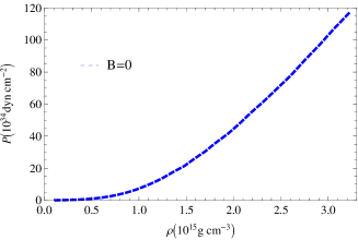
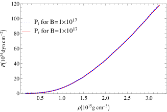
Figure 1: The equation of state of magnetized neutron matter for $B=0$ (left panel) and (right panel) the radial pressure and tangential pressure .vs density of magnetized neutron star for $B=1\times 10^{17}G$.

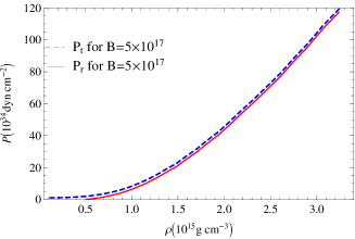
Figure 2: The radial pressure and tangential pressure .vs density of magnetized neutron star for $B=5\times 10^{17}G$ (left panel) and for $B=8\times 10^{17}G$ (right panel).

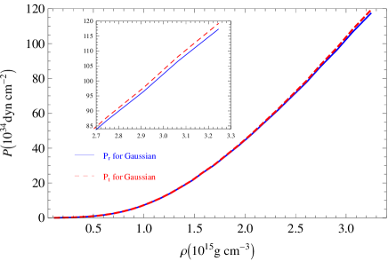
Figure 3: The radial pressure and tangential pressure .vs density of magnetized neutron star for Gaussian magnetic field.

Figure 4: The relative anisotropy parameter $\delta$ vs. magnetic field.

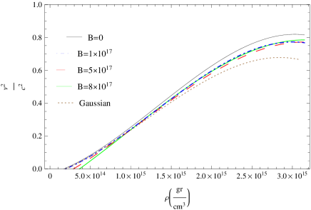
Figure 5: Sound speed vs. density

III Structure of anisotrop magnetized neutron star

In astrophysics, Tolman-Oppenheimer-Volkoff (TOV) equations expresses the structure of an object with a spherical symmetry that is in hydrostatic equilibrium TVO1 ; TVO2 ; TVO3 ,

$$\frac{dP}{dr}=-\frac{Gm(r)\rho(r)}{r^{2}}\left(1+\frac{P(r)}{\rho(r)c^{2}}\right)\left(1+\frac{4\pi r^{3}P(r)}{m(r)c^{2}}\right)\left(1-\frac{2Gm(r)}{rc^{2}}\right)^{-1},$$ (18)

where $\rho(r)$ is the energy density, $G$ is the gravitational constant and

$$m(r)=\int_{0}^{r}4\pi r^{\prime 2}\rho(r^{\prime})dr^{\prime},$$ (19)

gives the gravitational mass inside a radius $r$. For the anisotropic case we use the generalized TOV equation as follows Riazi ; Ponce ,

$$\frac{dP_{r}}{dr}=-\frac{Gm(r)\rho(r)}{r^{2}}\biggl{(}1+\frac{P_{r}}{\rho(r)c^{2}}\biggr{)}\biggl{(}1+\frac{4\pi r^{3}P_{r}}{m(r)c^{2}}\biggr{)}\biggl{(}1-\frac{2Gm(r)}{rc^{2}}\biggr{)}^{-1}+\frac{2\Delta}{r},$$ (20)

where we already defined $\Delta$ in previous section. By selecting a central energy density $\rho_{c}$, under the boundary conditions $P_{r}(0)=P_{c}$, $m(0)=0$, we integrate the TOV equations outwards to a radius $r=R$, at which $P_{r}$ vanishes. This yields the radius $R$ and gravitational mass $M=m(R)$ of the star.

The effects of magnetic fields on the gravitational mass of anisotrop neutron star for different $B$ values are presented in Figures 6 and 7 where the gravitational mass has been drawn versus the central mass density and radius ($M-R$ relation) respectively for different cases of magnetic field. As the magnetic field increases, the gravitational mass increases. From our results, in the absence of magnetic field, $B=0$, $M_{max}=1.68M_{\odot}$ and $R=9km$ have been obtained. In the presence of a uniform magnetic field, for $B=1\times 10^{17}G$, $M_{max}=1.92M_{\odot}$ and $R=9.8km$ have been evaluated, while for $B=5\times 10^{17}G$, $M_{max}=2.05M_{\odot}$ and $R=9.8km$ obtained. Also for $B=8\times 10^{17}G$, we have obtained $M_{max}=2.11M_{\odot}$ and $R=9.9km$. For Gaussian magnetic field, our calculations lead to $M_{max}=2.09M_{\odot}$, $R=10.03km$. Also it should be noted that the above results for the masses obey the stability conditions that will be examined in the next sections.

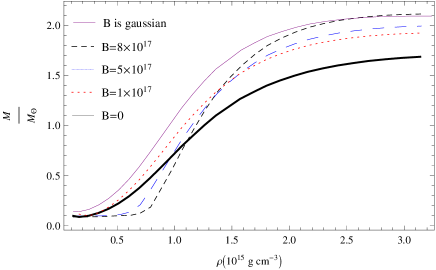
Figure 6: Gravitational mass vs. density for different magnetic fields.

Figure 7: Gravitational mass vs. radius for different magnetic fields.

Table 1: Properties of neutron star with different magnetic fields.

$B(G)$	${M_{max}}\ (M_{\odot})$	$R\ (km)$	$R_{Sch}\ (km)$	$\sigma(\frac{R_{Sch}}{R})$	$z$	$K(10^{-7}$ $m^{-2})$	$\frac{4c^{2}R}{9G}\ (M_{\odot})$
$0$	$1.68$	$9.00$	$4.93$	$0.56$	$0.51$	$0.20$	$2.63$
$1\times 10^{17}$	$1.92$	$9.80$	$5.63$	$0.57$	$0.53$	$0.21$	$2.95$
$5\times 10^{17}$	$2.05$	$9.80$	$6.01$	$0.61$	$0.61$	$0.22$	$2.96$
$8\times 10^{17}$	$2.11$	$9.90$	$6.20$	$0.63$	$0.64$	$0.24$	$2.99$
$Gaussian$	$2.09$	$10.03$	$6.13$	$0.61$	$0.60$	$0.22$	$3.00$

We have given some results for the properties of neutron star in Table 1. In order to make more investigation for anisotrop neutron star, we discuss about the Schwarzschild radius, compactness, redshift, Kretschmann scalar and Buchdahl-Bondi bound in the following sections.

III.1 Schwarzschild Radius

We obtain the Schwarzschild radius for the obtained masses in each magnetic field. To find the Schwarzschild radius of neutron stars, we use the relation $R_{Sch}=\frac{2GM}{c^{2}}$. By obtaining the Schwarzschild Radius we have found the maximum amount of Schwarzschild Radius as $R_{Sch}=6.2km$. This shows that our system can not be a black hole, and it is surely a neutron star because our result for the radius is greater than Schwarzschild Radius. The results indicate that by increasing the magnetic field, the Schwarzschild radius increases (see Table 1 for more details).

III.2 Compactness

The compactness is a very important quantity for neutron stars, and expresses the strength of the surface gravitational field. One of the important quantities which we want to investigate is related to the compactness of a spherical object. It can be defined as $\sigma=\frac{R_{Sch}}{R}$, which may be interpreted as the strength of gravity. Our results from Table 1 confirm that by increasing the magnetic field, the compactness increases.

III.3 Redshift

Another known parameter of neutron stars is the gravitational redshift. The surface gravitational redshift of a neutron star is closely connected to the value of $\frac{M}{R}$, with $M$ being the mass and $R$ the corresponding radius. The gravitational redshift of a neutron star is given by $z=\frac{1}{\sqrt{1-\frac{2GM}{c^{2}R}}}-1$. In Table 1, we see that the maximum value of redshift is for $B=8\times 10^{17}G$, $\sigma=0.63$. We see that these redshift values are allowed. We can see that increasing the magnetic field leads to increasing of the redshift.

III.4 Kretschmann scalar

When we study any space time, it is important above other things to know whether the spacetime is regular or not. By regular spacetime, we simply mean that the space time must have regular curvature invariants are finite at all spacetime points, or contain curvature singularities at which at least one such singularity is infinite. In the Schwarzschild metric, the components of the Ricci tensor $(R_{\mu\nu})$ and the Ricci scalar $(R)$ are zero outside the star, and these quantities do not give us any information about the spacetime curvature. Therefore, we use another quantity in order to further investigate the curvature of spacetime. The quantity that can help us to understand the curvature of spacetime is the Riemann tensor. The Riemann tensor may have more components, then for simplicity, we can study the Kretschmann scalar for measurement of the curvature in a vacuum. Therefore, the curvature at the surface of a neutron star is given as $K=\sqrt{R_{\mu\nu\alpha\beta}R^{\mu\nu\alpha\beta}}=\frac{4\sqrt{3}GM}{c^{2}R^{3}}$. The numerical results have been shown in Table 1 where we can see that the maximum of curvature is $8.3\times 10^{-8}(m^{-2})$. Also we have found that by increasing the magnetic field, the strength of gravity increases.

III.5 Buchdahl-Bondi bound

Here, we want to investigate the upper mass limit of a static spherical neutron star with uniform density in GR, the so-called Buchdahl theorem. The GR compactness limit is given by $M_{BB}\leqslant\frac{4c^{2}R}{9G}$ Buchdahl1 ; Buchdahl2 ; Buchdahl3 , in which the upper mass limit is $M_{max}=\frac{4c^{2}R}{9G}$. The results of our calculations confirm that the obtained masses of magnetic neutron stars are smaller than this limit and our system can not be a black hole.

III.6 Dynamical Stability

The virial relation for an equilibrium configuration, as suggested by Chandrasekhar and Fermi Chandrasekhar can be written as

$$3(\gamma-1)\epsilon_{k}+\epsilon_{B}+\epsilon_{G}=0,$$ (21)

where $\epsilon_{k}$ is the total kinetic energy of the system, $\epsilon_{B}$ is the positive magnetic energy due to magnetic field and $\epsilon_{G}$ is the negative gravitational potential and $\gamma$ is the adiabatic index defined as $\gamma=\frac{\rho c^{2}+P}{c^{2}P}\frac{dP}{d\rho}$. The total energy of the system is given by $E=\epsilon_{k}+\epsilon_{B}+\epsilon_{G}$, using Eq.(21), the total energy can be written as

$$E=-\frac{3\gamma-4}{3(\gamma-1)}(|\epsilon_{G}|-\epsilon_{B}).$$ (22)

For stability, the necessary condition is $E<0$, or

$$(3\gamma-4)|\epsilon_{G}|(1-\frac{\epsilon_{B}}{|\epsilon_{G}|})>0.$$ (23)

To satisfy this condition, first we should have $\gamma>\frac{4}{3}$, in order to investigate the dynamical stability of a magnetized neutron star, we plot the adiabatic index versus the radius in Figure 8. As one can see, these stars enjoy interior dynamical stability. Second condition is that the magnetic energy should not exceed the potential of gravity ($\epsilon_{B}>|\epsilon_{G}|$), because star is no longer stable or gravitationally unbound. Upper limit of stability is $\epsilon_{B}=|\epsilon_{G}|$. To investigate this condition, the magnetic energy is given by

$$\epsilon_{B}=\frac{B^{2}R^{3}}{6},$$ (24)

and the gravitational potential is given by

$$\epsilon_{G}=-\frac{3}{4}\frac{GM^{2}}{R}.$$ (25)

Using Eqs.(24) and (25) into stability condition, we can obtain the maximum value of magnetic field $B_{max}$ when the star can be stable

$$B_{max}=\sqrt{\frac{9G}{2}}\frac{M}{R^{2}}.$$ (26)

In our work for the maximum mass $M=2.11M_{\odot}$ and radius $R=9.9km$, it is found that $B_{max}=9.35\times 10^{17}G$. By using Eqs.(24), (25) and (26), we can drive the following condition for stability

$$\frac{\epsilon_{B}}{|\epsilon_{G}|}=\frac{B^{2}}{B_{max}^{2}}.$$ (27)

The values $\frac{B}{B_{max}}$, indicate that the predicted internal magnetic field $B$ always be lower than the magnetic field $B_{max}$ needed for stability. Due to this and that the maximum value of our magnetic field which was $B=8\times 10^{17}G$, the condition of stability is satisfied.

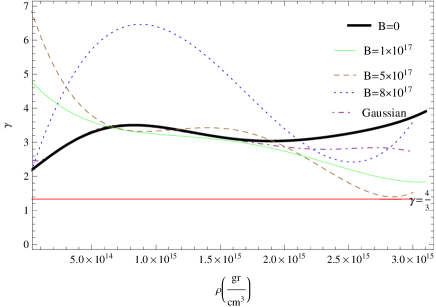
Figure 8: adiabatic index vs. density for different magnetic fields.

IV Comparison between Theory and Observations

One of the interesting features of our calculations is related to the comparison of the theory and its predictions with the observational data. For this purpose, we compare our results with the empirical evidence of the neutron stars. We present some observational data for $4U1608-52$ Guver , $VelaX-1$ Rawls , $PSRJ1614-2230$ Demorest , $PSRJ0348+0432$Antoniadis and $PSRJ0740+6620$ Cromartie in Table 2. According to Table 2 we can see that for $PSRJ1614-2230$, $PSRJ0348+0432$ and $PSRJ0740+6620$, the results of the Gaussian magnetic field are more consistent with the observational results, also for $VelaX-1$ and $4U1608-52$, the results for the case where the field is uniform are more consistent for $B=8\times 10^{17}G$ and $B=5\times 10^{17}G$, respectively.

It should be noted that obtaining the radius by observational measurement is difficult and complex. Here, according to Figure 7, we find radius corresponding to the observational mass for different magnetic fields, and we present this comparison in Table 3. Because our computational mass is smaller than the observational mass for some magnetic fields, the corresponding radius is not recorded for these values. Given the values obtained from the observations for the mass of the following objects (Table 2), we can claim that the results obtained from the theory are in agreement with the observational results. These results are much more accurate and closer to the observational data when we consider the magnetic field as Gaussian.

Table 2: Comparison of our results for the mass and radius of anisotrop neutron stars with those of observation.

$Name$	${M}\ (M_{\odot})$	$R\ (km)$	$Our\ work$	${M}\ (M_{\odot})$	$R\ (km)$
$PSRJ0740+6620$	$2.10$	$12(\pm 2)$	$For\ Gaussian$	$2.09$	$10.03$
$PSRJ0348+0432$	$2.01$	$13(\pm 2)$	$For\ B=8\times 10^{17}G$	$2.11$	$9.90$
$PSRJ1614-2230$	$1.97$	$12(\pm 2)$	$For\ B=5\times 10^{17}G$	$2.05$	$9.80$
$Vela$X-1	$1.80$	$11(\pm 2)$	$For\ B=1\times 10^{17}G$	$1.92$	$9.80$
$4U1608-52$	$1.74$	$9(\pm 1)$	$For\ B=0$	$1.68$	$9.00$

Table 3: Radius corresponding to observational mass .

Observational	Observational	Radius for	Radius for	Radius for	Radius for
Object	mass ${M}\ (M_{\odot})$	$B=1\times 10^{17}G$	$B=5\times 10^{17}G$	$B=8\times 10^{17}G$	Gaussian
		$\ (km)$	$\ (km)$	$\ (km)$	$\ (km)$
$PSRJ0740+6620$	$2.10$	$-$	$-$	$10.00$	$10.50$
$PSRJ0348+0432$	$2.01$	$-$	$10.20$	$10.40$	$10.95$
$PSRJ1614-2230$	$1.97$	$-$	$10.30$	$10.55$	$11.20$
$Vela$X-1	$1.80$	$10.56$	$10.58$	$10.75$	$11.55$
$4U1608-52$	$1.74$	$10.80$	$10.60$	$10.80$	$11.60$

V Conclusions

In this paper we studied the structure of anisotropic neutron stars. For this purpose, we calculated the equation of state of magnetized neutron star that contains pure neutron matter in the presence of an strong magnetic field. For computation of anisotropic pressure, we considered two type of magnetic field. In the first case, $B$ is constant from the center to the surface of the neutron star, and calculations were performed for four fixed values of magnetic fields. In the second case, we used a Gaussian function to define density dependent magnetic field where the maximum amount of magnetic field is in the center of the star and decreases as it moves to the surface of the star. Using the obtained equation of state, we integrated the generalized TOV equation to compute the structure of anisotrop neutron star. We showed that by increasing the magnetic field, the maximum mass of neutron star increases. For the maximum magnetic field $B=8\times 10^{17}G$, the maximum amount of mass was obtained as $M_{max}=2.11M_{\odot}$. We also examined the stability of this star, where we showed that the adiabatic index is higher than $\gamma=\frac{4}{3}$, and the star is also stable in our computational magnetic fields. By considering different values of magnetic fields, we evaluated compactness, redshift and the Kretschmann scalar for these compact objects. Our results indicate that these quantities are increasing functions of magnetic field strength. Finally, we compared our theoretical results with the observational data, and it was shown that our theoretical results are in agreement with the empirical evidence of neutron stars.

- (1) M. Camenzind, Compact Objects in Astrophysics: White Dwarfs, Neutron Stars and Black Holes Springer,Verlag Berlin Heidelberg ( 2007).
- (2) A. Reisenegger, Astron. Nachr. 328, 1173 (2007).
- (3) L. Woltjer, Astrophys. J. 140, 1309 (1964).
- (4) D. Lai and S. L. Shapiro, Astrophys. J. 383, 745 (1991).
- (5) E. J. Ferrer, V. de la Incera, J. P. Keith, I. Portillo, and P. L. Springsteen, Phys. Rev. C 82, 065802 (2010).
- (6) V. Canuto and H. Y. Chiu, Phys. Rev. 173, 1210 (1968).
- (7) A. Broderick, M. Prakash, and J. M. Lattimer, Astrophys. J. 537, 351 (2000).
- (8) S. Fayazbakhsh, and N. Sadooghi, Phys. Rev. D 90, 105030 (2014).
- (9) A. M. Abrahams, and S. L. Shapiro, Astrophys. J. 374, 652 (1991).
- (10) I. -S. Suh, and G. J. Mathews, Astrophys. J. 546, 1126 (2001).
- (11) A. Perez-Martinez, H. Perez-Rojas, and H. J. Mosquera-Cuesta, Eur. Phys. J. C 29, 111 (2003).
- (12) A. Broderick, M. Prakash, and J. M. Lattimer, Phys. Lett. B 531, 167 (2002).
- (13) G. Mao, A. Iwamoto, and Z. Li, Chin. J. Astron. Astrophys. 3, 359 (2003).
- (14) R. G. Felipe, A. P. Martinez, H. P. Rojas, and M. Orsaria, Phys. Rev. C 77, 015807 (2008).
- (15) P. Yue, F. Yang, and H. Shen, Phys. Rev. C 79, 025803 (2009).
- (16) V. Dexheimer, R. Negreiros, and S. Schramm, Eur. Phys. J. A 48, 189 (2012).
- (17) J. Dong, U. Lombardo, W. Zuo, and H. Zhang, Nucl. Phys. A 898, 32 (2013).
- (18) R. H. Casali, L. B. Castro, and D. P. Menezes, Phys. Rev. C 89, 015805 (2014).
- (19) R. D. Blandford, J. H. Applegate and L. Hernquist, Mon. Not. R. Astron. Soc. 204, 1025 (1983).
- (20) J. A. Pons, and U. Geppert, Astron. Astrophys 470, 303 (2007).
- (21) M. Sinha, and B. Mukhopadhyay, Nucl. Phys. A 898, 43 (2013).
- (22) K. Chatziioannou, Gen. Rel. Grav. 52, 109 (2020).
- (23) G. Lematre, Ann. Soc. Sci. Bruxelles A 53, 51 (1933).
- (24) R. L. Bowers, and E. P. T. Liang, Astrophys. J. 188, 657 (1974).
- (25) Z. Roupas, and G. G. L. Nashed, Eur. Phys. J. C 80, 905 (2020).
- (26) L. Herrera, Phys. Rev. D 101, 104024 (2020).
- (27) G. H. Bordbar, and M. Hayati, Int. J. Mod. Phys. A 21, 1555 (2006).
- (28) T. Yazdizadeh, and G. H. Bordbar, Res. Astron. Asrtophys. 11, 471 (2011).
- (29) B. Eslam Panah, T. Yazdizadeh, and G. H. Bordbar, Eur. Phys. J. C 79, 815 (2019).
- (30) S. H. Hendi, G. H. Bordbar, B. Eslam Panah, and M. Najafi, Astrophys Space Sci. 358, 30 (2015).
- (31) G. H. Bordbar, S. H. Hendi, and B. Eslam Panah, Eur. Phys. J. Plus. 131, 315 (2016).
- (32) S. H. Hendi, G. H. Bordbar, B. Eslam Panah, and S. Panahiyan, JCAP 09, 013 (2016).
- (33) S. H. Hendi, G. H. Bordbar, B. Eslam Panah, and S. Panahiyan, JCAP 07, 004 (2017).
- (34) G. H. Bordbar, Z. Rezaei, and A. Montakhab, Phys. Rev. C 83, 044310 (2011).
- (35) B. Eslam Panah, G. H. Bordbar, S. H. Hendi, R. Ruffini, Z. Rezaei, and R. Moradi, Astrophys. J. 848, 24 (2017).
- (36) G. H. Bordbar, and Z. Rezaei, Phys. Lett. B 718, 1125 (2012).
- (37) D. Bandyopadhyay, S. Chakrabarty, and S. Pal, Phys. Rev. Lett. 79, 2176 (1997).
- (38) R. Mallick, and S. Schramm, Phys. Rev. C 89, 045805 (2014).
- (39) I. Tews, J. Carlson, S. Gandolfi, and S. Reddy, Astrophys. J. 860, 149 (2018).
- (40) R. C. Tolman, Proc. Natl. Acad. Sci. 20, 169 (1934).
- (41) R. C. Tolman, Phys. Rev. 55, 364 (1939).
- (42) J. R. Oppenheimer, and G. M. Volkoff, Phys. Rev. 55, 374 (1939).
- (43) J. W. Clark, Prog. Part. Nucl. Phys. 2, 89 (1979).
- (44) R. B. Wiringa, V. Stoks, and R. Schiavilla, Phys. Rev. C 51, 38 (1995).
- (45) G. H. Bordbar and M. Modarres, Phys. Rev. C 57, 714 (1998).
- (46) J. Ponce de Leon, General Relativity and Gravitation, 25, 1123, (1993).
- (47) N. Riazi, S. S. Hashemi, S. N. Sajadi, and Sh. Assyyaee, Can. J. Phys. 94, 1093 (2016).
- (48) H. A. Buchdahl, Phys. Rev. 116, 1027 (1959).
- (49) H. Bondi, Proc. R. Soc. London A 282, 303 (1964).
- (50) H. A. Buchdahl, Astrophys. J. 146, 275 (1966).
- (51) S. Chandrasekhar and E. Fermi, Astrophys. J. 118 116 (1953).
- (52) T. Guver, F.Ozel, A. Cebrera-Lavers, and P. Wroblewski, Astrophys. J. 712, 964 (2010).
- (53) M. L. Rawls, J. A. Orosz, J. E. McClintock, et al. Astrophys. J. 25, 730 (2011).
- (54) P. Demorest, T. Pennucci, S. Ransom, M. Roberts and J. Hessels, Nature 467, 1081 (2010).
- (55) J. Antoniadis, P. C. C. Freire, N. Wex, et al. Sci, 340, 6131 (2013).
- (56) H. T. Cromartie, E. Fonseca, S. M. Ransom, P. B. Demorest, Z. Arzoumanian, et al., Nat. Astron. 4, 72 (2020).