Can late-time extensions solve the $H_{0}$ and $\sigma_{8}$ tensions?

Abstract

We analyze the properties that any late-time modification of the $\Lambda$CDM expansion history must have in order to consistently solve both the $H_{0}$ and the $\sigma_{8}$ tensions. Taking a model-independent approach, we obtain a set of necessary conditions that can be applied to generic late-time extensions. Our results are fully analytical and merely based on the assumptions that the deviations from the $\Lambda$CDM background remain small. For the concrete case of a dark energy fluid with equation of state $w(z)$, we derive the following general requirements: (i) Solving the $H_{0}$ tension demands $w(z)<-1$ at some $z$ (ii) Solving both the $H_{0}$ and $\sigma_{8}$ tensions requires $w(z)$ to cross the phantom divide. Finally, we also allow for small deviations on the effective gravitational constant. In this case, our method is still able to constrain the functional form of these deviations.

I Introduction

Historically, the quest for a satisfactory description of our universe has always been guided by the latest observational data. It is therefore not surprising that the dramatic increase of the quantity and quality of cosmological observations over the last 25 years has allowed for a revolution on the theoretical side as well. The $\Lambda$CDM model has emerged as the leading theoretical description of cosmic evolution, explaining key features, such as the distribution of the cosmic microwave background (CMB) anisotropies, with only a few free parameters. However, despite its success, several observations have been, and still are, hard to account for within this paradigm. In particular, the well-known $H_{0}$ tension, that is the discrepancy of the Hubble constant inferred from the CMB within $\Lambda$CDM Aghanim et al. (2020) compared to the results of local measurements Riess et al. (2019); Pesce et al. (2020); Wong et al. (2020); Riess et al. (2021), has become increasingly worrying in recent years and it is hard to disregard it as a simple statistical fluke. At this point, either there is something wrong with different, independent observations or we must change the theoretical framework to interpret them.

Another mayor concern in the community is the $\sigma_{8}$ tension which, just as the $H_{0}$ tension, arises when comparing the CMB-inferred value of the clustering amplitude to alternative observations, in this case large scale structure (LSS) surveys Abbott et al. (2018, 2021); Asgari et al. (2021); Heymans et al. (2021). Focusing on these two parameters and disregarding correlations with other parameters, we may say that CMB data favors a lower value of $H_{0}$ while at the same time preferring a higher $\sigma_{8}$ value compared to late-time measurements. See Nunes and Vagnozzi (2021) for a compilation of recent measurements.

In recent years, great efforts have been made towards solving the $H_{0}$ tension, see e.g. Poulin et al. (2019); Smith et al. (2020); Alcaniz et al. (2021); Zumalacarregui (2020); Gómez-Valent et al. (2020); Ballesteros et al. (2020); Jiménez et al. (2021); Di Valentino et al. (2021a); Banerjee et al. (2021); Krishnan et al. (2021); Teng et al. (2021); Ballardini et al. (2021); Braglia et al. (2021, 2020), as well as the $\sigma_{8}$ tension, see e.g. Lambiase et al. (2019); Keeley et al. (2019); Di Valentino et al. (2020); Jedamzik et al. (2021); Clark et al. (2021); Solà Peracaula et al. (2021); Alestas and Perivolaropoulos (2021); Nunes and Vagnozzi (2021); Schöneberg et al. (2021); Alestas et al. (2021); Ye et al. (2021) (see also Riess (2019); Knox and Millea (2020); Di Valentino et al. (2021b, c, d); Perivolaropoulos and Skara (2021) for an overview of observations and models). Among these solutions, those that modify the behaviour of dark energy either at late or early times have received special attention. Both run into similar problems when trying to solve the Hubble tension while being consistent with complementary observations, and in this work we will restrict ourselves to late-time models. Typical late-time solutions to the $H_{0}$ tension, as for example models based on scalar or vector Galileons Renk et al. (2017); Frusciante et al. (2020); de Felice et al. (2017); De Felice et al. (2020); Heisenberg and Villarrubia-Rojo (2021), usually lead to an even larger value of $\sigma_{8}$ than within $\Lambda$CDM and therefore potentially increase the $\sigma_{8}$ tension. One should however keep in mind that the $\sigma_{8}$ tension is only properly addressed as a tension in the $\sigma_{8}$-$\Omega_{m}$ plane, or in the general multidimensional posterior. While these models predict a slightly larger $\sigma_{8}$ they also prefer smaller values for $\Omega_{m}$, a result in the line of weak-lensing surveys. However, even if one could argue that strictly speaking such late-time solutions to the Hubble tension are still statistically compatible with current $\sigma_{8}$ measurements, they clearly show the wrong trend, such that they will most likely be difficult to reconcile with a low $\sigma_{8}$ value if it is confirmed by the more precise measurements of the next generation of LSS surveys.

This generic trend, that late-time dark energy models easing the Hubble tension predominantly increase $\sigma_{8}$ as well, can be understood as follows. A realistic dark energy model typically affects $\sigma_{8}$ in two ways: 1) Through its effects on the expansion history, i.e. modifications of the background equation of state. 2) Through its clustering properties, i.e. clustering dark energy that can modify the effective Newton constant $G_{\text{eff}}$ which governs the evolution of the matter growth function. In the models mentioned above with a phantom equation of state both effects contribute to an increase in $\sigma_{8}$: 1) A phantom-like evolution of dark energy extends the matter-dominated phase, boosting the matter growth. 2) Dark energy clusters at late times, increasing $G_{\text{eff}}$ and further boosting the amplitude of perturbations. The key point is that the same phantom-like equation of state that is crucial to solve the $H_{0}$ tension, can only worsen the $\sigma_{8}$ tension.

In face of these problems, one may wonder if it is even possible to solve both tensions modifying only the late-time dark energy behavior. Of course, in a consistent dark energy model one should not only study the background evolution, but the perturbations as well. And while the background evolution is governed by the dark energy equation of state $w(z)$, the perturbations are also affected by the dark energy sound speed $c_{\text{s}}(z)$. Hence, at first sight one could conclude that with two arbitrary functions at hand it should not be difficult to find a dark energy model that solves both tensions at once. However, this is not the case since in realistic scenarios such as vector Galileons both functions are not independent and their observational impact is very different. In fact, while $c_{\text{s}}(z)$ is relevant for observables like the ISW effect, the modifications in $w(z)$ are the main force driving the values of $\sigma_{8}$ and $H_{0}$. In the light of these considerations we will therefore narrow down the scope of this work by mostly neglecting the effects of dark energy perturbations and address the following main question:

Can the $H_{0}$ and $\sigma_{8}$ tensions be simultaneously relieved modifying only the dark energy equation of state $w(z)$ at late times?

We will show that the answer is no if the dark energy equation of state does not meet some very definite criteria. These conclusions apply to any dark energy model in which the perturbations do not play a leading role in the determination of $\sigma_{8}$. After this, we will generalize the results to the case where dark energy also affects the growth of structure through a change in the effective gravitational constant. Thus, our results provide valuable insights into the behavior of the dark sector and can be seen as hints towards building successful models beyond $\Lambda$CDM.

The main steps of the computation can be succintly summarized as follows:

1. We will start off with a late-time $\Lambda$CDM cosmology, that can effectively be described by two free parameters $\big{(}h,\omega_{m}\big{)}$, i.e. the Hubble constant and the matter abundance. In a second step, we consider an alternative cosmology with slightly different parameters and with a different expansion history $\big{(}h+\delta h,\omega_{m}+\delta\omega_{m},\delta H(z)\big{)}$. Here, $\delta H(z)$ is an arbitrary function that produces a small deformation of the $\Lambda$CDM expansion history, for fixed $h$ and $\omega_{m}$. Restricting ourselves to late time modifications translates into the assumption that $\delta H(z)=0$ for roughly $z>300$. With all the deformations considered to be small, the Hubble parameter in the alternative cosmology can be written as

   $$H=H_{\text{\tiny$\Lambda$CDM}}+\Delta H\big{(}\delta h,\delta\omega_{m},\delta H(z)\big{)}\ .$$ (1)

2. Working to first order, we compute the variations induced by the modified Hubble parameter in different cosmological observables.

3. Because of the deformation $\delta H(z)$, the observationally preferred values for $h$ and $\omega_{m}$ in the new cosmology will be different compared to the initial $\Lambda$CDM model. The variations $\delta h$ and $\delta\omega_{m}$ can be related to $\delta H(z)$ by choosing two very well measured observables whose value should not change in the new cosmology, i.e. we impose their variation to be zero in order to be compatible with observations. This allows to compute the response functions

   $$\frac{\delta h}{h} =\int\mathcal{R}_{h}(z)\frac{\delta H(z)}{H(z)}\frac{\text{d}z}{1+z}\ ,$$ (2a)

   $$\frac{\delta\omega_{m}}{\omega_{m}} =\int\mathcal{R}_{\omega_{m}}(z)\frac{\delta H(z)}{H(z)}\frac{\text{d}z}{1+z}\ .$$ (2b)

   In this work we will choose the variations of the CMB distance priors Chen et al. (2019) to vanish. The response functions $\mathcal{R}_{h}$ and $\mathcal{R}_{\omega_{m}}$ are fully analytical and are defined in (22).

4. Based on the results above we can then compute the response function of any other quantity, and crucially in our case

   $$\frac{\Delta\sigma_{8}}{\sigma_{8}}=\int\mathcal{R}_{\sigma_{8}}(z)\frac{\delta H(z)}{H(z)}\frac{\text{d}z}{1+z}\ .$$ (3)

   Depending on the shape of the response functions, this allows to derive general requirements on the functional form of $\delta H(z)$ in order to achieve the desired variations in $h$ and $\sigma_{8}$. Again, $\mathcal{R}_{\sigma_{8}}$ can be computed analytically and it will be derived in Section IV.

5. In Section IV.3, we will generalize these results and include a second free function, $\delta G_{\text{eff}}(z)$, that affects the evolution of $\sigma_{8}$, computing its associated response function along the same lines.

This paper is organized as follows. In Section II we introduce the deformations of the background and most of the notation. Section III will cover the choice of observational data (CMB priors) used to compute the response functions. Section IV deals with the variations of the growth factor and $\sigma_{8}$. It also includes a generalization for models that modify the effective Newton constant. In Section V we address the resolution of the $H_{0}$ tension in more detail, analyzing the differences that arise when formulated in terms of the supernova absolute magnitude $M$. Section VI summarizes the results of this work. Appendix A collects all the analytical formulae used to derive the results in the main text. Finally, in Appendix B we present some tests performed to check the accuracy of the first-order, analytical results against the full numerical computation with a Boltzmann code for a particular dark energy model.

II Deformations of the expansion history

The Hubble parameter in $\Lambda$CDM can be written as

$$H^{2}_{\text{\tiny$\Lambda$CDM}} =H_{0}^{2}\Big{(}\Omega_{m}(1+z)^{3}+\Omega_{r}(1+z)^{4}+\Omega_{\Lambda}\Big{)}$$

$$=C_{H}^{2}\Big{(}\omega_{m}(1+z)^{3}+\omega_{r}(1+z)^{4}+\omega_{\Lambda}\Big{)}\ ,$$ (4)

where $C_{H}\equiv 100\ \text{km}\,\text{s}^{-1}\,\text{Mpc}^{-1}$ and

$$\omega_{\Lambda}=h^{2}-\omega_{m}-\omega_{r}\ .$$ (5)

Let us consider now a generic extension that slightly modifies the expansion history, for fixed values of all the cosmological parameters, so the new Hubble parameter is

$$H(h,\omega_{m})=H_{\text{\tiny$\Lambda$CDM}}(h,\omega_{m})+\delta H\ .$$ (6)

This deformation of the expansion history will also shift the preferred values for the $\Lambda$CDM parameters, by a small amount. The observationally preferred background in $\Lambda$CDM and in the generic extension can then be related as

$$H(h+\delta h,\omega_{m}+\delta\omega_{m})=H_{\text{\tiny$\Lambda$CDM}}(h,\omega_{m})+\Delta H\ ,$$ (7)

where we are also assuming that $\delta H$ only produces late-time changes so the cosmology can be effectively described by $h$ and $\omega_{m}$. Assuming that all these variations are small and working to first order we have

$$\frac{\Delta H}{H}=\frac{H_{0}^{2}}{H^{2}}\frac{\delta h}{h}+m(z)\frac{\delta\omega_{m}}{\omega_{m}}+\frac{\delta H}{H}\ ,\qquad\quad m(z)\equiv\frac{\Omega_{m}H_{0}^{2}}{2H^{2}}\left((1+z)^{3}-1\right)\ .$$ (8)

Starting with the general variation (8), we can propagate its effect to any cosmological observable. In general, for every cosmological quantity $g(z)$ we will express its variation as

$$\frac{\Delta g(z)}{g(z)}=I_{g}(z)\frac{\delta h}{h}+J_{g}(z)\frac{\delta\omega_{m}}{\omega_{m}}+\int^{\infty}_{0}\frac{\text{d}x_{z}}{1+x_{z}}R_{g}(x_{z},z)\frac{\delta H(x_{z})}{H(x_{z})}\ .$$ (9)

For instance, from the definition of the conformal, luminosity and angular diameter distances,

$$\chi(z) =\int^{z}_{0}\frac{\text{d}z}{H(z)}\ ,$$ (10a)

$$d_{L}(z) =(1+z)\chi(z)\ ,$$ (10b)

$$d_{A}(z) =\frac{1}{1+z}\chi(z)\ ,$$ (10c)

we can easily compute

$$\left\{\begin{array}[]{l}\displaystyle I_{\chi}(z)=I_{d_{L}}(z)=I_{d_{A}}(z)=-\frac{1}{\chi(z)}\int^{z}_{0}\text{d}x_{z}\frac{H_{0}^{2}}{H^{3}}\ ,\\[8.0pt] \displaystyle J_{\chi}(z)=J_{d_{L}}(z)=J_{d_{A}}(z)=-\frac{1}{\chi(z)}\int^{z}_{0}\text{d}x_{z}\frac{H_{0}^{2}}{H^{3}}m(x_{z})\ ,\\[8.0pt] \displaystyle R_{\chi}(x_{z},z)=R_{d_{L}}(x_{z},z)=R_{d_{A}}(x_{z},z)=-(1+x_{z})\frac{\theta(z-x_{z})}{\chi(z)H(x_{z})}\ .\end{array}\right.$$ (11)

Notice that, since we are working to first order, every function like $\chi(z)$ and $H(z)$ can be computed in the base $\Lambda$CDM cosmology. The full analytical expressions for all the $(I,J,R)$ functions that are used in this work are collected in Appendix A.

Finally, notice that we can also express the previous results in terms of a variation on the energy content

$$H^{2}(h,\omega_{m})=H^{2}_{\text{\tiny$\Lambda$CDM}}(h,\omega_{m})+H_{0}^{2}\delta\Omega\ .$$ (12)

Working again to first order we have

$$\frac{\delta H}{H}=\frac{H_{0}^{2}}{2H^{2}}\delta\Omega\ .$$ (13)

Note that we did not, and will not, specify a functional form for either $\delta H$ or $\delta\Omega$. However, in particular models some additional properties may be desirable. For instance, if $\delta\Omega$ arises from a dark energy model, we may want to require that the dark energy density is positive, leading to

$$\Omega_{\text{DE}}(z)\equiv\Omega_{\Lambda}+\delta\Omega(z)>0\qquad\text{(DE model)}$$ (14)

In this case, we can also relate the variation to the equation of state of dark energy $w(z)$

$$\delta\Omega(z)=\Omega_{\Lambda}\left\{\exp\left(3\int^{z}_{0}\big{(}1+w(z)\big{)}\frac{\text{d}z}{1+z}\right)-1\right\}\ .$$ (15)

Following the same reasoning, in a model with dark matter and dark energy interactions we have

$$\Omega_{\text{DE-DM}}(z)\equiv\Omega_{\Lambda}+\Omega_{\text{cdm}}(1+z)^{3}+\delta\Omega(z)>0\qquad\text{(Interacting DM-DE model)}$$ (16)

III CMB priors and the $H_{0}$ tension

In the previous section we considered a generic background modification over a $\Lambda$CDM cosmology. However, we know that the extremely precise observations of the CMB severely restrict such modifications. Two combinations of parameters are particularly well measured,

$$\theta_{*} \equiv\frac{r_{\text{s}}(z_{*})}{(1+z_{*})d_{A}(z_{*})}\ ,$$ (17a)

$$R_{*} \equiv(1+z_{*})d_{A}(z_{*})\sqrt{\Omega_{m}H_{0}^{2}}\ .$$ (17b)

where $r_{s}(z)$ is the comoving sound horizon

$$r_{\text{s}}(z)=\int^{\infty}_{z}\frac{\text{d}z}{H}c_{\text{s}}\ ,\qquad c_{\text{s}}=\frac{1}{\sqrt{3(1+R)}}\ ,\qquad R=\frac{3\Omega_{b}}{4\Omega_{\gamma}(1+z)}\ ,$$ (18)

and $z_{*}\simeq 1090$ is the redshift at decoupling, see Chen et al. (2019) for a more accurate interpolation formula. These are commonly referred to as the CMB distance priors: the acoustic scale ($\theta_{*}$) and the shift parameter ($R_{*}$), that govern the angular position and the relative heights of the peaks, respectively. Their latest values using the Planck 2018 release, for $\Lambda$CDM and some extensions, can be found in Chen et al. (2019). We can compute their variation following the steps of the previous section

$$\frac{\Delta\theta_{*}}{\theta_{*}} =\frac{\Delta r_{\text{s}}^{*}}{r_{\text{s}}^{*}}-\frac{\Delta d_{A}^{*}}{d_{A}^{*}}\ ,$$ (19a)

$$\frac{\Delta R_{*}}{R_{*}} =\frac{\Delta d_{A}^{*}}{d_{A}^{*}}+\frac{\delta\omega_{m}}{2\omega_{m}}\ .$$ (19b)

Here we are using the short-hand notation $d_{A}^{*}\equiv d_{A}(z_{*})$. The variation in these two parameters is only a small fraction of all the possible changes that any modified cosmology can produce in the CMB. If we want to compute all these changes and definitively establish the level of agreement of a given model with the CMB, we must resort to a Boltzmann code and perform the numerical computation. However, we can argue that in order not to be directly excluded, any reasonable $\Lambda$CDM extension must keep $\theta_{*}$ and $R_{*}$ approximately fixed. Then, imposing $\Delta\theta_{*},\Delta R_{*}\simeq 0$, we obtain the following system

$$\left(I_{d_{A}}^{*}-I_{r_{\text{s}}}^{*}\right)\frac{\delta h}{h}+\left(J_{d_{A}}^{*}-J_{r_{\text{s}}}\right)\frac{\delta\omega_{m}}{\omega_{m}} =\int\frac{\text{d}x_{z}}{1+x_{z}}\left(R^{*}_{r_{\text{s}}}-R^{*}_{d_{A}}\right)\frac{\delta H}{H}\ ,$$ (20a)

$$I_{d_{A}}^{*}\frac{\delta h}{h}+\left(J_{d_{A}}^{*}+\frac{1}{2}\right)\frac{\delta\omega_{m}}{\omega_{m}} =-\int^{\infty}_{0}\frac{\text{d}x_{z}}{1+x_{z}}R^{*}_{d_{A}}\frac{\delta H}{H}\ .$$ (20b)

Solving the system we get the response functions for $h$ and $\omega_{m}$

$$\frac{\delta h}{h} =\int^{\infty}_{0}\frac{\text{d}x_{z}}{1+x_{z}}\,\mathcal{R}_{h}(x_{z})\frac{\delta H(x_{z})}{H(x_{z})}\ ,$$ (21a)

$$\frac{\delta\omega_{m}}{\omega_{m}} =\int^{\infty}_{0}\frac{\text{d}x_{z}}{1+x_{z}}\,\mathcal{R}_{\omega_{m}}(x_{z})\frac{\delta H(x_{z})}{H(x_{z})}\ .$$ (21b)

where

$$\mathcal{R}_{h} =\frac{1}{D_{*}}\left\{\left(J_{d_{A}}^{*}+\frac{1}{2}\right)\left(R_{r_{\text{s}}}(x,z_{*})-R_{d_{A}}(x,z_{*})\right)-(I^{*}_{r_{\text{s}}}-I^{*}_{d_{A}})R_{d_{A}}(x,z_{*})\right\}\ ,$$ (22a)

$$\mathcal{R}_{\omega_{m}} =\frac{1}{D_{*}}\Big{\{}I^{*}_{r_{\text{s}}}R_{d_{A}}(x,z_{*})-I_{d_{A}}^{*}R_{r_{\text{s}}}(x,z_{*})\Big{\}}\ ,$$ (22b)

$$D^{*} =I^{*}_{d_{A}}\left(J^{*}_{r_{\text{s}}}-J^{*}_{d_{A}}\right)-\left(I^{*}_{r_{\text{s}}}-I^{*}_{d_{A}}\right)\left(J^{*}_{d_{A}}+\frac{1}{2}\right)\ .$$ (22c)

The response functions allow us to connect the changes produced in the expansion history by a generic model with changes of the observationally preferred parameters in the new cosmology. The observations considered in this case are the CMB priors, which ensure that all the modified cosmologies considered are roughly compatible with the CMB. While the expressions derived so far are general, we will restrict ourselves to late-time modifications, so that $\delta H(z)=0$ for $z>300$.

We can now use the previous results to compute the response function of any other cosmological quantity

$$\frac{\Delta\mathcal{G}(z)}{\mathcal{G}(z)}=\int^{\infty}_{0}\frac{\text{d}x_{z}}{1+x_{z}}\,\mathcal{R}_{\mathcal{G}}(x_{z},z)\frac{\delta H(x_{z})}{H(x_{z})}\ ,$$ (23)

where the response function $\mathcal{R}_{\mathcal{G}}$ can be expressed as

$$\mathcal{R}_{\mathcal{G}}(x_{z},z)\equiv I_{\mathcal{G}}(z)\mathcal{R}_{h}(x_{z})+J_{\mathcal{G}}(z)\mathcal{R}_{\omega_{m}}(x_{z})+R_{\mathcal{G}}(x_{z},z)\ .$$ (24)

These results allow us to answer one of the main questions of this work. The response function $\mathcal{R}_{h}$, depicted in Figure 2, is strictly negative, so to increase the value of $h$ and thus solve the Hubble tension we need $\delta H(z)<0$ for some $z$. In the context of dark energy models, according to (15), this means that the equation of state must be phantom-like, i.e. $w(z)<-1$ for some $z$. To reach this conclusion we only used the fact that $\mathcal{R}_{h}$ is strictly negative. Its shape will be important in the next section, where we will try to simultaneously solve the $H_{0}$ and the $\sigma_{8}$ tensions.

Finally, the response function of $\omega_{m}$ is very close to zero in the whole range $0<z<300$. Even though we will present the analytical results with full generality, for late-time modifications it is completely justified to keep $\omega_{m}$ fixed, i.e. $\mathcal{R}_{\omega_{m}}\to 0$. The variation of the Hubble parameter can then be obtained using only the first CMB prior in (19)

$$\frac{\delta h}{h}\simeq-\frac{1}{I^{*}_{d_{A}}}\int^{\infty}_{0}\frac{\text{d}x_{z}}{1+x_{z}}R^{*}_{d_{A}}\frac{\delta H}{H}\ .$$ (25)

IV Growth factor and the $\sigma_{8}$ tension

IV.1 Growth factor and $\sigma_{8}$ in $\Lambda$CDM

After decoupling, the time evolution of matter perturbations can be encapsulated in the growth factor. The growth factor in $\Lambda$CDM obeys

$$\frac{\text{d}^{2}D}{\text{d}a^{2}}+\frac{\text{d}\log(a^{3}H)}{\text{d}a}\frac{\text{d}D}{\text{d}a}-F(a)D=0\ ,\qquad F(a)\equiv\frac{3\Omega_{m}H^{2}_{0}}{2a^{5}H^{2}}\ .$$ (26)

This equation remains valid even if the expansion history $H(a)$ is different from $\Lambda$CDM, as long as the equations describing the perturbations are not modified. For a late-time $\Lambda$CDM universe, where matter and $\Lambda$ are the dominant components, the two independent solutions of (26) can be expressed analitically

$$D_{+}(a) =\frac{5\Omega_{m}}{2}\frac{H(a)}{H_{0}}I(a)\ ,\qquad I(a)\equiv\int^{a}_{0}\text{d}x_{a}\frac{H_{0}^{3}}{\big{(}x_{a}H(x_{a})\big{)}^{3}}\ ,$$ (27a)

$$D_{-}(a) \propto H(a)\ ,$$ (27b)

where $D_{+}$ and $D_{-}$ are the growing and decaying mode, respectively. It is also common to define the linear growth rate $f$, that in $\Lambda$CDM can be approximated as

$$f\equiv\frac{\text{d}\log{D_{+}}}{\text{d}\log a}\simeq\left(\frac{\Omega_{m}H_{0}^{2}a^{-3}}{H^{2}}\right)^{0.55}.$$ (28)

We start with the definition, e.g. see Dodelson and Schmidt (2020),

$$\sigma_{R}^{2}\equiv\left\langle\delta^{2}_{m,R}(\boldsymbol{x})\right\rangle\ ,$$ (29)

where

$$\delta_{m,R}(\boldsymbol{x})\equiv\int\text{d}^{3}x^{\prime}\,\delta_{m}(\boldsymbol{x}^{\prime})W_{R}\big{(}|\boldsymbol{x}-\boldsymbol{x}^{\prime}|\big{)}\ ,\qquad W_{R}\big{(}r\big{)}=\left\{\begin{array}[]{ll}\displaystyle\frac{3}{4\pi R^{3}}\ ,&\quad x<R\\[8.0pt] 0\ ,&\quad x>R\end{array}\right.$$ (30)

It is common practice to evaluate this averaged clustering amplitude in spheres of radius $R=8\ h^{-1}\text{Mpc}$ and denote it as $\sigma_{8}$. It can be equivalently expressed in Fourier space and in terms of the matter power spectrum as

$$\sigma_{R}^{2}=\int\frac{\text{d}k}{k}\mathcal{P}_{m}(k)W^{2}(kR)\ ,\qquad W(x)\equiv\frac{3j_{1}(x)}{x}\ ,$$ (31)

where $j_{1}$ is a spherical Bessel function. The approximate form of the linear matter power spectrum in terms of the matter growth factor and the transfer function is Dodelson and Schmidt (2020)

$$\mathcal{P}_{m}(k)\equiv\frac{k^{3}}{2\pi^{2}}P_{m}(k)=\frac{4}{25}\frac{k^{4}}{\Omega_{m}^{2}H_{0}^{4}}T^{2}(k)D^{2}_{+}(a)\mathcal{P}_{\mathcal{R}}(k)\ ,$$ (32)

where the primordial power spectrum of curvature perturbations is

$$\mathcal{P}_{\mathcal{R}}(k)=A_{s}\left(\frac{k}{k_{p}}\right)^{n_{s}-1},\qquad k_{p}=0.05\,\text{Mpc}^{-1}\ .$$ (33)

For the transfer function we will adopt the Eisenstein-Hu fitting formula Eisenstein and Hu (1998) that takes into account the baryonic supression at small scales and proves important for an accurate computation of $\sigma_{8}$. Following the notation of the original work Eisenstein and Hu (1998)

$$q =\frac{k}{\text{Mpc}^{-1}}\frac{\Theta_{2.7}^{2}}{\Gamma_{\text{eff}}}\ , \qquad\qquad\Gamma_{\text{eff}} =\omega_{m}\left(\alpha_{\Gamma}+\frac{1-\alpha_{\Gamma}}{1+(0.43ks)^{4}}\right)\ ,$$

$$T_{0}(q) =\frac{L_{0}}{L_{0}+C_{0}q^{2}}\ , \qquad\qquad\alpha_{\Gamma} =1-0.328\log(431\omega_{m})\frac{\omega_{b}}{\omega_{m}}+0.38\log(22.3\omega_{m})\left(\frac{\omega_{b}}{\omega_{m}}\right)^{2}\ ,$$

$$L_{0}(q) =\log(2\text{e}+1.8q)\ , \qquad\qquad s =\frac{44.5\log(9.83/\omega_{m})}{\sqrt{1+10(\omega_{b})^{3/4}}}\,\text{Mpc}\ ,$$

$$C_{0}(q) =14.2+\frac{731}{1+62.5q}\ ,$$ (34)

where $\Theta_{2.7}$ is the temperature of the CMB in $2.7\ \text{K}$ units. So finally, the transfer function that we will use is $T_{\text{EH}}(k)=T_{0}\big{(}q(k)\big{)}$ Also notice that we will always assume that $k$ in the integral is measured in $\text{Mpc}^{-1}$ and not in $\text{Mpc}^{-1}\,h$ units. After rewriting (31), we can write the $\sigma_{8}$ as

$$\sigma_{8}^{2}=\frac{4}{25\omega_{m}}D_{+}^{2}(a)\mathcal{I}_{k}\ ,$$ (35)

where

$$\mathcal{I}_{k}=\int^{\infty}_{0}\frac{\text{d}k}{k}\left(\frac{k}{C_{H}}\right)^{4}T^{2}(k)W^{2}(kR)\mathcal{P}_{\mathcal{R}}(k)\ ,$$ (36)

and again $R=8\ h^{-1}\text{Mpc}$. Closely related, $S_{8}$ is defined as

$$S_{8}\equiv\sigma_{8}\sqrt{\frac{\Omega_{m}}{0.3}}\ .$$ (37)

This quantity is closer to what is actually measured in weak-lensing surveys and is commonly used to reformulate the $\sigma_{8}$ tension as a $S_{8}$ tension. Spectroscopic surveys on the other hand usually target the combination $f\sigma_{8}$, that can be precisely measured with redshift-space distortions.

IV.2 The $\sigma_{8}$ tension

The evolution of the variation of the growth factor is described by

$$\frac{\text{d}^{2}}{\text{d}a^{2}}\Delta D+\frac{\text{d}\log(a^{3}H)}{\text{d}a}\frac{\text{d}}{\text{d}a}\Delta D-F(a)\Delta D=g(a)\ ,$$ (38)

where

$$g(a)\equiv-\frac{\text{d}}{\text{d}a}\left(\frac{\Delta H}{H}\right)\frac{\text{d}D}{\text{d}a}+FD\left(\frac{\delta\omega_{m}}{\omega_{m}}-2\frac{\Delta H}{H}\right)\ .$$ (39)

Using the Wronskian method, we can construct the particular solution to the inhomogeneous equation (38) and express the variations of the growth factor and the linear growth rate as

$$\Delta D =\frac{H(a)}{H_{0}}\int^{a}_{0}\text{d}x_{a}\frac{x_{a}^{3}H^{2}(x_{a})}{H_{0}^{2}}\Big{(}I(a)-I(x_{a})\Big{)}g(x_{a})\ ,$$ (40)

$$\Delta f =\frac{\text{d}}{\text{d}\log a}\frac{\Delta D}{D}\ .$$ (41)

The full analytical expressions for the $(I,J,R)$ pieces of the variations can be found in Appendix A. We are now in position to compute the variation in the $\sigma_{8}$ clustering amplitude. This variation can be written as the combination

$$\frac{\Delta\sigma_{8}}{\sigma_{8}}=\frac{\Delta D}{D}-\frac{\delta\omega_{m}}{\omega_{m}}+\frac{1}{2}\frac{\Delta\mathcal{I}_{k}}{\mathcal{I}_{k}}\ .$$ (42)

We still need to compute the variations on the integral $\mathcal{I}_{k}$

$$\Delta\mathcal{I}_{k} =2\int^{\infty}_{0}\frac{\text{d}k}{k}T^{2}(k)\left(\frac{k}{C_{H}}\right)^{4}W(kR)\Delta W(kR)\mathcal{P}_{\mathcal{R}}(k)$$

$$\quad+2\int^{\infty}_{0}\frac{\text{d}k}{k}T(k)\Delta T(k)\left(\frac{k}{C_{H}}\right)^{4}W^{2}(kR)\mathcal{P}_{\mathcal{R}}(k)\ .$$ (43)

Similarly, the variation of $S_{8}$ is

$$\frac{\Delta S_{8}}{S_{8}}=\frac{\Delta\sigma_{8}}{\sigma_{8}}-\frac{\delta h}{h}+\frac{1}{2}\frac{\delta\omega_{m}}{\omega_{m}}\ .$$ (44)

The response functions for $\sigma_{8}$, $f\sigma_{8}$ and $S_{8}$ are represented in Figure 2. Both $\mathcal{R}_{\sigma_{8}}$ and $\mathcal{R}_{f\sigma_{8}}$ are strictly negative, which means that in order to reduce them we need $\delta H(z)>0$ at some $z$. This can be compared with the result of the previous section, which showed that in order to increse $H_{0}$ we need $\delta H(z)<0$. The bottom line of this analysis is that both conditions must be fulfilled to solve the two cosmological tensions, otherwise we improve one at the cost of worsening the other. In particular, for a dark energy model (15) a change of sign in $\delta H(z)$ implies that the equation of state $w(z)$ must cross the value $w=-1$. However, the results for $S_{8}$ are slightly different, since at very late-times the response function changes its sign. This feature could be very positive if, with the results of upcoming LSS surveys, we find ourselves in a situation where the clustering amplitude tension is clearly more severe in $S_{8}$ or in $f\sigma_{8}$. The different behaviour of their response functions might be then a clear explanation and could give us hints about the shape of $\delta H(z)$.

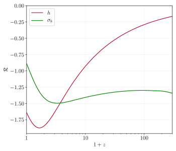
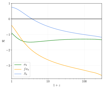
Figure 1: (Left) Response functions for $h$ and $\sigma_{8}$. Notice that both have the same sign so, unless $\delta H$ changes sign, both variations follow the same trend, i.e. if we increase $h$ we also increase $\sigma_{8}$. (Right) Response functions for other clustering-related quantities.

IV.3 Deformations beyond the background: $G_{\text{eff}}$

We define $G_{\text{eff}}$ as a modification in the sub-Hubble regime that leads to the modified evolution for the growth factor

$$\frac{\text{d}^{2}D}{\text{d}a^{2}}+\frac{\text{d}\log(a^{3}H)}{\text{d}a}\frac{\text{d}D}{\text{d}a}-\frac{G_{\text{eff}}}{G}F(a)D=0\ .$$ (45)

Many realistic scenarios actually produce this kind of modification, e.g. see Heisenberg and Villarrubia-Rojo (2021). Following the same steps as in previous sections, if we assume that the effective gravitational coupling is close to the $\Lambda$CDM case, $G_{\text{eff}}=G+\delta G(z)$, we get

$$\frac{\text{d}^{2}}{\text{d}a^{2}}\Delta D+\frac{\text{d}\log(a^{3}H)}{\text{d}a}\frac{\text{d}}{\text{d}a}\Delta D-F(a)\Delta D=F(a)D(a)\frac{\delta G(a)}{G}\ ,$$ (46)

where in this case $\Delta D$ stands for a variation keeping fixed all the cosmological parameters and $H(z)$. The particular solution is

$$\frac{\Delta D}{D} =\frac{H(a)}{D(a)H_{0}}\int^{a}_{0}\text{d}x_{a}\frac{x_{a}^{3}H^{2}(x_{a})}{H_{0}^{2}}\Big{(}I(a)-I(x_{a})\Big{)}F(x_{a})D(x_{a})\frac{\delta G(x_{a})}{G}$$

$$=\int^{\infty}_{0}\frac{\text{d}x_{z}}{1+x_{z}}\mathcal{G}(x_{z},z)\frac{\delta G(x_{z})}{G}\ ,$$ (47)

where the response function for $\delta G$ is

$$\mathcal{G}(x_{z},z)=\frac{H^{3}(z)D(x_{z})}{H_{0}^{3}D(z)}\Big{(}I(z)-I(x_{z})\Big{)}F(x_{z})\frac{\theta(x_{z}-z)}{(1+x_{z})^{4}}\ .$$ (48)

Since we are working to first order, the complete variation, modifying the background as well, is just a linear combination with the results of the previous section, i.e.

$$\frac{\Delta D}{D}\bigg{\lvert}_{\text{full}}=\int^{\infty}_{0}\frac{\text{d}x_{z}}{1+x_{z}}\left(\mathcal{R}_{D}(x_{z},z)\frac{\delta H(x_{z})}{H(x_{z})}+\mathcal{G}(x_{z},z)\frac{\delta G(x_{z})}{G}\right)\ .$$ (49)

Including two free functions $\delta H(z)$ and $\delta G(z)$ make the results more general but unfortunately prevent us from making strong statements about the behaviour of any of them. In order to proceed further, we restrict ourselves to the case in which $\delta H(z)$ does not change sign. We know that this scenario is realized in many physically relevant models, for instance when we have a dark energy fluid that does not cross the phantom divide.

We already discussed that in this case in order to solve the $H_{0}$ tension we require $\delta H<0$. If we do not modify the evolution of the perturbations, i.e. $G_{\text{eff}}=G$, this leads to an increase in $\sigma_{8}$, since $\mathcal{R}_{\sigma_{8}}<0$. However, including $\delta G(z)$ we have enough freedom to increase $H_{0}$ while reducing $\sigma_{8}$. Intuitively, it seems evident that we can achieve this goal just reducing the effective strength of gravity enough, i.e. $\delta G(z)<0$. Defining $\alpha(x_{z})\equiv-\mathcal{R}_{\sigma_{8}}(x_{z},0)/\mathcal{G}(x_{z},0)$ and using the previous results we can derive the stronger condition

$$\frac{\delta G(x_{z})}{G}<\alpha(z)\frac{\delta H(x_{z})}{H(x_{z})}<0\qquad\text{for some }x_{z}>0\ ,$$ (50)

that a model must satisfy if we want to reduce the value of $\sigma_{8}$, while increasing $H_{0}$.

V Supernova absolute magnitude

Most discussions on the Hubble tension are formulated in terms of the $H_{0}$, or $h$, parameter. However, the parameter that is closer to what is actually measured by collaborations like SH0ES Riess et al. (2019), is the absolute magnitude $M$ used to calibrate the observed apparent magnitudes of SNe. This is the actual source of the Hubble tension, as has been stressed by Camarena and Marra (2021), which also presented models where $H_{0}$ is raised without affecting $M$. In this section we will compute the response function for $M$, paying special attention to its differences with respect to the response function for $h$. The apparent magnitude and distance modulus are defined as Scolnic et al. (2018)

$$m \equiv 5\log_{10}\left(\frac{d_{L}}{\text{Mpc}}\right)+25+M\ ,$$ (51)

$$\mu \equiv m-M\ ,$$ (52)

where $M$ is the absolute magnitude, that must be calibrated to infer the distance from the observed apparent magnitude. The $\chi^{2}$ can then be constructed as

$$\chi^{2}_{\text{\tiny{SNe}}}=(m_{\text{obs}}^{i}-m_{\text{th}}^{i})(C^{-1})_{ij}(m_{\text{obs}}^{j}-m_{\text{th}}^{j})\ ,$$ (53)

and it can be analitically minimized for $M$

$$\frac{\partial\chi^{2}_{\text{\tiny{SNe}}}}{\partial M}=0\qquad\to\qquad M_{\text{best\ fit}}=\frac{\sum_{ij}(C^{-1})_{ij}(m_{\text{obs}}^{j}-\mu_{\text{th}}^{j})}{\sum_{ij}(C^{-1})_{ij}}\ .$$ (54)

For given values of $H_{0}$ and $\Omega_{m}$, this is the absolute magnitude that provides the best fit to SNe data. Its variation is

$$\Delta M=-5\frac{\delta h}{h}-\frac{5}{\sum_{ij}(C^{-1})_{ij}}\sum_{ij}\frac{(C^{-1})_{ij}\Delta d_{L}(z_{j})}{d_{L}(z_{j})}\ ,$$ (55)

so we have

$$\mathcal{R}_{M}(x_{z})=-5\mathcal{R}_{h}(x_{z})-\frac{5}{\sum_{ij}(C^{-1})_{ij}}\sum_{ij}(C^{-1})_{ij}\mathcal{R}_{d_{L}}(x_{z},z_{j})\ .$$ (56)

In this work, we will use the Pantheon sample Scolnic et al. (2018) for the computation of (56). In Figure 2, we can see that, in contrast with $h$, the response function for $M$ changes sign at low redshift. This means that models that rely on modifications at very low redshift may increase the Hubble constant without actually decreasing $M$, a result in line with the conclusions of Camarena and Marra (2021).

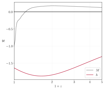
Figure 2: (Left) Response of $\sigma_{8}$ to small changes in the effective gravitational constant, $\mathcal{G}$ in (48). The second curve $\alpha(z)$ depicts the bound defined in (50). (Right) Response function of $h$ and the supernova absolute magnitude $M$. Notice that the latter becomes negative at very low redshift, so a very late-time modification that tries to increase the value of $h$ would also increase $M$ and thus fail at addressing the $H_{0}$ tension between the CMB and supernovae-based direct measurements.

VI Summary and conclusions

In this paper we have addressed the question of why typical late-time dark energy models only solve the $H_{0}$ tension at the cost of predicting a large clustering amplitude $\sigma_{8}$ and whether it is therefore actually possible to relieve both tensions simultaneously by perturbatively modifying the expansion history, and maybe the gravitational constant, at late times. Using a model independent approach we derived a set of necessary conditions on the functional form of $\delta H(z)$ which have to be satisfied in order to tackle both the $H_{0}$ and $\sigma_{8}$ tensions. For the particularly interesting case in which the deformation is due to dark energy with equation of state $w(z)$ our results can be summarized schematically as follows

1. Solving the $H_{0}$ tension $\quad\Rightarrow\quad$ $\delta H(z)<0$ for some $z$ $\quad\Rightarrow\quad$ $w(z)<-1$ for some $z$.

2. If the perturbations are not modified ($G_{\text{eff}}=G$) then:
   Solving the $H_{0}$ and $\sigma_{8}$ tensions $\quad\Rightarrow\quad$ $\delta H(z)$ changes sign $\quad\Rightarrow\quad$ $w(z)$ crosses the phantom divide.

3. If $G_{\text{eff}}=G+\delta G(z)$ and $\delta H(z)$ does not change sign then:
   Solving the $H_{0}$ and $\sigma_{8}$ tensions $\quad\Rightarrow\quad$ $\displaystyle\frac{\delta G(z)}{G}<\alpha(z)\frac{\delta H(z)}{H(z)}<0\quad$ for some $z$.
   where $\delta H(z)<0$ and $\alpha(z)>0$.

4. Solutions that rely on significant modifications at low redshift ($z<1$) can increase $H_{0}$ without decreasing the supernova absolute magnitude $M$, thus failing to adress the Hubble tension.

Note that while we chose here to present the implications of our results for the specific case of a dark energy model, the conditions on the form of $\delta H(z)$ are much more general and can be applied to any theory.

Providing a full catalog of models ruled out by these necessary criteria will be left for future work, as well as the further study of theories meeting them. It would for example be interesting to include low redshift constraints from baryon acoustic oscillation (BAO) data and address concerns along the lines of Benevento et al. (2020).

Another interesting avenue would be to extend this results to early dark energy models. In this case, the CMB would be modified in a different way and different observational anchors should be used. The variation of $\omega_{m}$, negligible for this work, would have to be taken into account and would potentially play an important role.

Finally, while the computations in the present paper, in particular the solution (40), explicitly assume a $\Lambda$CDM background with only matter and curvature contributions on top of the cosmological constant, it is possible to generalize our analysis to arbitrary backgrounds. This will allow the application of the method to deviations from general DE models or theories beyond Einstein gravity and will be useful especially in the context of effective field theory of dark energy to consider observables at the perturbation level beyond $G_{\text{eff}}$ presented here.

Appendix A Full analytical results

This appendix contains the full analytical expressions used in this work. Unless otherwise stated, every function inside the integrals depends on the integration variable $x_{z}$. Comoving, luminosity and angular diameter distance:

$$\left\{\begin{array}[]{l}\displaystyle I_{\chi}(z)=I_{d_{L}}(z)=I_{d_{A}}(z)=-\frac{1}{\chi(z)}\int^{z}_{0}\text{d}x_{z}\frac{H_{0}^{2}}{H^{3}}\\[8.0pt] \displaystyle J_{\chi}(z)=J_{d_{L}}(z)=J_{d_{A}}(z)=-\frac{1}{\chi(z)}\int^{z}_{0}\text{d}x_{z}\frac{H_{0}^{2}}{H^{3}}m(x_{z})\\[8.0pt] \displaystyle R_{\chi}(x_{z},z)=R_{d_{A}}(x_{z},z)=R_{d_{A}}(x_{z},z)=-(1+x_{z})\frac{\theta(z-x_{z})}{\chi(z)H(x_{z})}\end{array}\right.$$ (57)

Comoving sound horizon:

$$\left\{\begin{array}[]{l}\displaystyle I_{r_{\text{s}}}(z)=-\frac{1}{r_{\text{s}}(z)}\int^{\infty}_{z}\text{d}x_{z}\frac{H_{0}^{2}}{H^{3}}c_{\text{s}}(x_{z})\\[8.0pt] \displaystyle J_{r_{\text{s}}}(z)=-\frac{1}{r_{\text{s}}(z)}\int^{\infty}_{z}\text{d}x_{z}\frac{H_{0}^{2}}{H^{3}}m(x_{z})c_{\text{s}}(x_{z})\\[8.0pt] \displaystyle R_{r_{\text{s}}}(x_{z},z)=-\frac{(1+x_{z})c_{\text{s}}(x_{z})}{r_{\text{s}}(z)}\frac{\theta(x_{z}-z)}{H(x_{z})}\end{array}\right.$$ (58)

Integral defined in (36):

$$\left\{\begin{array}[]{l}\displaystyle I_{\mathcal{I}_{k}}=-\frac{2}{\mathcal{I}_{k}}\int^{\infty}_{0}\frac{\text{d}k}{k}T^{2}(k)\mathcal{P}_{\mathcal{R}}(k)\left(\frac{k}{C_{H}}\right)^{4}kR\,W(kR)W^{\prime}(kR)\\[8.0pt] \displaystyle J_{\mathcal{I}_{k}}=\frac{2\omega_{m}}{\mathcal{I}_{k}}\int^{\infty}_{0}\frac{\text{d}k}{k}T(k)\frac{\partial T(k)}{\partial\omega_{m}}\mathcal{P}_{\mathcal{R}}(k)\left(\frac{k}{C_{H}}\right)^{4}W^{2}(kR)\\[8.0pt] \displaystyle R_{\mathcal{I}_{k}}=0\end{array}\right.$$ (59)

Growth factor:

$$\left\{\begin{array}[]{l}\displaystyle I_{D}(z)=-\frac{H(z)}{H_{0}D(z)}\int^{\infty}_{z}\frac{\text{d}x_{z}}{1+x_{z}}\frac{H_{0}^{2}D}{H^{2}}\Bigg{\{}\frac{H_{0}}{H}f+\frac{N(z,x_{z})F}{1+x_{z}}\left(1+\frac{(1+x_{z})^{3}}{F}\frac{\text{d}\log H}{\text{d}x_{z}}f\right)\Bigg{\}}\\[8.0pt] \displaystyle J_{D}(z)=\frac{1}{5}+\frac{H(z)}{H_{0}D(z)}\int^{\infty}_{z}\frac{\text{d}x_{z}}{(1+x_{z})^{2}}N(z,x_{z})FD\\ \displaystyle\qquad\qquad-\frac{H(z)}{H_{0}D(z)}\int^{\infty}_{z}\frac{\text{d}x_{z}}{1+x_{z}}mD\Bigg{\{}\frac{H_{0}}{H}f+\frac{N(z,x_{z})F}{1+x_{z}}\left(1+\frac{(1+x_{z})^{3}}{F}\frac{\text{d}\log H}{\text{d}x_{z}}f\right)\Bigg{\}}\\[8.0pt] \displaystyle R_{D}(x_{z},z)=-\frac{H(z)D(x_{z})}{H_{0}D(z)}\Bigg{\{}\frac{H_{0}}{H(x_{z})}f(x_{z})+\frac{N(z,x_{z})F(x_{z})}{1+x_{z}}\left(1+\frac{(1+x_{z})^{3}}{F(x_{z})}\frac{\text{d}\log H}{\text{d}x_{z}}f(x_{z})\right)\Bigg{\}}\theta(x_{z}-z)\end{array}\right.$$ (60)

Linear growth rate:

$$\left\{\begin{array}[]{l}\displaystyle I_{f}(z)=-I_{D}(z)\left(1+\frac{1+z}{f}\frac{\text{d}\log H}{\text{d}z}\right)-\frac{H_{0}^{2}}{H^{2}(z)}\\[8.0pt] \displaystyle\qquad\qquad-\frac{(1+z)^{2}H_{0}^{2}}{f(z)H^{2}(z)D(z)}\int^{\infty}_{z}\frac{\text{d}x_{z}}{(1+x_{z})^{5}}FD\left(1+\frac{(1+x_{z})^{3}}{F}\frac{\text{d}\log H}{\text{d}x_{z}}f\right)\\[8.0pt] \displaystyle J_{f}(z)=-\left(J_{D}(z)-\frac{1}{5}\right)\left(1+\frac{1+z}{f}\frac{\text{d}\log H}{\text{d}z}\right)-m(z)\\[8.0pt] \displaystyle\qquad\qquad+\frac{(1+z)^{2}}{f(z)H^{2}(z)D(z)}\int^{\infty}_{z}\frac{\text{d}x_{z}}{(1+x_{z})^{5}}H^{2}FD\Big{\{}1-m\left(1+\frac{(1+x_{z})^{3}}{F}\frac{\text{d}\log H}{\text{d}x_{z}}f\right)\Big{\}}\\[8.0pt] \displaystyle R_{f}(x_{z},z)=-R_{D}(x_{z},z)\left(1+\frac{1+z}{f}\frac{\text{d}\log H}{\text{d}z}\right)-\delta(x_{z}-z)\\[8.0pt] \displaystyle\qquad\qquad\qquad-\frac{1}{(1+z)f(z)}\frac{(1+z)^{3}H^{2}(x_{z})D(x_{z})}{(1+x_{z})^{3}H^{2}(z)D(z)}\frac{F(x_{z})}{1+x_{z}}\left(1+\frac{(1+x_{z})^{3}}{F(x_{z})}\frac{\text{d}\log H}{\text{d}x_{z}}f(x_{z})\right)\theta(x_{z}-z)\end{array}\right.$$ (61)

Supernova absolute magnitude:

$$\left\{\begin{array}[]{l}\displaystyle I_{M}=-\frac{5}{M}-\frac{5}{M\sum_{ij}(C^{-1})_{ij}}\sum_{ij}(C^{-1})_{ij}I_{\chi}(z_{j})\\[8.0pt] \displaystyle J_{M}=-\frac{5}{M\sum_{ij}(C^{-1})_{ij}}\sum_{ij}(C^{-1})_{ij}J_{\chi}(z_{j})\\[8.0pt] \displaystyle R_{M}(x_{z})=-\frac{5}{M\sum_{ij}(C^{-1})_{ij}}\sum_{ij}(C^{-1})_{ij}R_{\chi}(x_{z},z_{j})\end{array}\right.$$ (62)

Appendix B Numerical benchmarks

The analytical expressions of the previous section have been tested for two particular dark energy models, $w=\text{const.}$ and the CPL Chevallier and Polarski (2001); Linder (2003) parameterization $w=w_{0}+w_{a}(1-a)$. In the latter, we choose fix parameter $w_{0}=-1.05$ to obtain a deformation $\delta H(z)$ that changes sign at late times. We compare the analytical results with the numerical ones obtained using class Blas et al. (2011), keeping fixed the acoustic scale $\theta_{*}$ and $\omega_{m}$. The analytic results show a very satisfactory performance as can be seen in Tables 1 and 2.

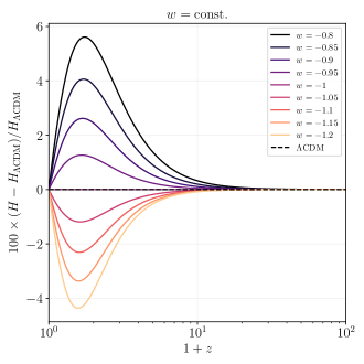
Figure 3: $\delta H(z)$ for two common dark energy parameterizations.

	$100\times\delta h/h$			$100\times\Delta\sigma_{8}/\sigma_{8}$
$w$	class	Analytical		class	Analytical
$-0.80$	$-8.57$	$-10.97$		$-8.98$	$-7.13$
$-0.85$	$-6.47$	$-7.76$		$-6.29$	$-5.32$
$-0.90$	$-4.35$	$-4.89$		$-3.93$	$-3.53$
$-0.95$	$-2.19$	$-2.32$		$-1.85$	$-1.76$
$-1.05$	$2.22$	$2.10$		$1.65$	$1.75$
$-1.10$	$4.47$	$4.01$		$3.12$	$3.48$
$-1.15$	$6.75$	$5.74$		$4.45$	$5.21$
$-1.20$	$9.07$	$7.33$		$5.66$	$6.93$

Table 1: Comparison of our analytical results with the full computation in class, keeping fixed $\theta_{*}$ and $\omega_{m}$, for a dark energy model with a constant equation of state $w$.

	$100\times\delta h/h$			$100\times\Delta\sigma_{8}/\sigma_{8}$
$w_{a}$	class	Analytical		class	Analytical
$-0.05$	$2.81$	$2.61$		$2.24$	$2.08$
$-0.01$	$2.35$	$2.22$		$1.86$	$1.75$
$0.03$	$1.89$	$1.80$		$1.47$	$1.39$
$0.07$	$1.42$	$1.37$		$1.07$	$1.03$
$0.11$	$0.946$	$0.93$		$0.66$	$0.64$
$0.14$	$0.465$	$0.46$		$0.24$	$0.23$
$0.174$	$0.095$	$0.093$		$-0.089$	$-0.092$
$0.18$	$-0.022$	$-0.025$		$-0.19$	$-0.20$
$0.22$	$-0.52$	$-0.53$		$-0.64$	$-0.65$
$0.26$	$-1.02$	$-1.07$		$-1.09$	$-1.13$
$0.3$	$-1.54$	$-1.62$		$-1.56$	$-1.64$

Table 2: Comparison of our analytical results with the full computation in class, keeping fixed $\theta_{*}$ and $\omega_{m}$, for a dark energy model with an equation of state $w(a)=-1.05+w_{a}(1-a)$. Notice that in this case $\delta H(z)$ changes sign, as shown in the right pannel in Figure 2, and for the case $w_{a}=0.174$ the variations have opposite signs. Even though they are too small to relieve the tensions, this example shows that when $\delta H(z)$ changes sign it is possible to increase $h$ while reducing $\sigma_{8}$.

References

- Aghanim et al. (2020) N. Aghanim et al. (Planck), Astron. Astrophys. 641, A6 (2020), [Erratum: Astron.Astrophys. 652, C4 (2021)], eprint 1807.06209.
- Riess et al. (2019) A. G. Riess, S. Casertano, W. Yuan, L. M. Macri, and D. Scolnic, Astrophys. J. 876, 85 (2019), eprint 1903.07603.
- Pesce et al. (2020) D. W. Pesce et al., Astrophys. J. Lett. 891, L1 (2020), eprint 2001.09213.
- Wong et al. (2020) K. C. Wong et al., Mon. Not. Roy. Astron. Soc. 498, 1420 (2020), eprint 1907.04869.
- Riess et al. (2021) A. G. Riess, S. Casertano, W. Yuan, J. B. Bowers, L. Macri, J. C. Zinn, and D. Scolnic, Astrophys. J. Lett. 908, L6 (2021), eprint 2012.08534.
- Abbott et al. (2018) T. M. C. Abbott et al. (DES), Phys. Rev. D 98, 043526 (2018), eprint 1708.01530.
- Abbott et al. (2021) T. M. C. Abbott et al. (DES) (2021), eprint 2105.13549.
- Asgari et al. (2021) M. Asgari et al. (KiDS), Astron. Astrophys. 645, A104 (2021), eprint 2007.15633.
- Heymans et al. (2021) C. Heymans et al., Astron. Astrophys. 646, A140 (2021), eprint 2007.15632.
- Nunes and Vagnozzi (2021) R. C. Nunes and S. Vagnozzi, Mon. Not. Roy. Astron. Soc. 505, 5427 (2021), eprint 2106.01208.
- Poulin et al. (2019) V. Poulin, T. L. Smith, T. Karwal, and M. Kamionkowski, Phys. Rev. Lett. 122, 221301 (2019), eprint 1811.04083.
- Smith et al. (2020) T. L. Smith, V. Poulin, and M. A. Amin, Phys. Rev. D 101, 063523 (2020), eprint 1908.06995.
- Alcaniz et al. (2021) J. Alcaniz, N. Bernal, A. Masiero, and F. S. Queiroz, Phys. Lett. B 812, 136008 (2021), eprint 1912.05563.
- Zumalacarregui (2020) M. Zumalacarregui, Phys. Rev. D 102, 023523 (2020), eprint 2003.06396.
- Gómez-Valent et al. (2020) A. Gómez-Valent, V. Pettorino, and L. Amendola, Phys. Rev. D 101, 123513 (2020), eprint 2004.00610.
- Ballesteros et al. (2020) G. Ballesteros, A. Notari, and F. Rompineve, JCAP 11, 024 (2020), eprint 2004.05049.
- Jiménez et al. (2021) J. B. Jiménez, D. Bettoni, and P. Brax, Phys. Rev. D 103, 103505 (2021), eprint 2004.13677.
- Di Valentino et al. (2021a) E. Di Valentino, A. Mukherjee, and A. A. Sen, Entropy 23, 404 (2021a), eprint 2005.12587.
- Banerjee et al. (2021) A. Banerjee, H. Cai, L. Heisenberg, E. O. Colgáin, M. M. Sheikh-Jabbari, and T. Yang, Phys. Rev. D 103, L081305 (2021), eprint 2006.00244.
- Krishnan et al. (2021) C. Krishnan, R. Mohayaee, E. O. Colgáin, M. M. Sheikh-Jabbari, and L. Yin, Class. Quant. Grav. 38, 184001 (2021), eprint 2105.09790.
- Teng et al. (2021) Y.-P. Teng, W. Lee, and K.-W. Ng, Phys. Rev. D 104, 083519 (2021), eprint 2105.02667.
- Ballardini et al. (2021) M. Ballardini, F. Finelli, and D. Sapone (2021), eprint 2111.09168.
- Braglia et al. (2021) M. Braglia, M. Ballardini, F. Finelli, and K. Koyama, Phys. Rev. D 103, 043528 (2021), eprint 2011.12934.
- Braglia et al. (2020) M. Braglia, M. Ballardini, W. T. Emond, F. Finelli, A. E. Gumrukcuoglu, K. Koyama, and D. Paoletti, Phys. Rev. D 102, 023529 (2020), eprint 2004.11161.
- Lambiase et al. (2019) G. Lambiase, S. Mohanty, A. Narang, and P. Parashari, Eur. Phys. J. C 79, 141 (2019), eprint 1804.07154.
- Keeley et al. (2019) R. E. Keeley, S. Joudaki, M. Kaplinghat, and D. Kirkby, JCAP 12, 035 (2019), eprint 1905.10198.
- Di Valentino et al. (2020) E. Di Valentino, A. Melchiorri, O. Mena, and S. Vagnozzi, Phys. Dark Univ. 30, 100666 (2020), eprint 1908.04281.
- Jedamzik et al. (2021) K. Jedamzik, L. Pogosian, and G.-B. Zhao, Commun. in Phys. 4, 123 (2021), eprint 2010.04158.
- Clark et al. (2021) S. J. Clark, K. Vattis, J. Fan, and S. M. Koushiappas (2021), eprint 2110.09562.
- Solà Peracaula et al. (2021) J. Solà Peracaula, A. Gómez-Valent, J. de Cruz Perez, and C. Moreno-Pulido, EPL 134, 19001 (2021), eprint 2102.12758.
- Alestas and Perivolaropoulos (2021) G. Alestas and L. Perivolaropoulos, Mon. Not. Roy. Astron. Soc. 504, 3956 (2021), eprint 2103.04045.
- Schöneberg et al. (2021) N. Schöneberg, G. Franco Abellán, A. Pérez Sánchez, S. J. Witte, V. Poulin, and J. Lesgourgues (2021), eprint 2107.10291.
- Alestas et al. (2021) G. Alestas, D. Camarena, E. Di Valentino, L. Kazantzidis, V. Marra, S. Nesseris, and L. Perivolaropoulos (2021), eprint 2110.04336.
- Ye et al. (2021) G. Ye, J. Zhang, and Y.-S. Piao (2021), eprint 2107.13391.
- Riess (2019) A. G. Riess, Nature Rev. Phys. 2, 10 (2019), eprint 2001.03624.
- Knox and Millea (2020) L. Knox and M. Millea, Phys. Rev. D 101, 043533 (2020), eprint 1908.03663.
- Di Valentino et al. (2021b) E. Di Valentino et al., Astropart. Phys. 131, 102604 (2021b), eprint 2008.11285.
- Di Valentino et al. (2021c) E. Di Valentino et al., Astropart. Phys. 131, 102605 (2021c), eprint 2008.11284.
- Di Valentino et al. (2021d) E. Di Valentino, O. Mena, S. Pan, L. Visinelli, W. Yang, A. Melchiorri, D. F. Mota, A. G. Riess, and J. Silk, Class. Quant. Grav. 38, 153001 (2021d), eprint 2103.01183.
- Perivolaropoulos and Skara (2021) L. Perivolaropoulos and F. Skara (2021), eprint 2105.05208.
- Renk et al. (2017) J. Renk, M. Zumalacárregui, F. Montanari, and A. Barreira, JCAP 10, 020 (2017), eprint 1707.02263.
- Frusciante et al. (2020) N. Frusciante, S. Peirone, L. Atayde, and A. De Felice, Phys. Rev. D 101, 064001 (2020), eprint 1912.07586.
- de Felice et al. (2017) A. de Felice, L. Heisenberg, and S. Tsujikawa, Phys. Rev. D 95, 123540 (2017), eprint 1703.09573.
- De Felice et al. (2020) A. De Felice, C.-Q. Geng, M. C. Pookkillath, and L. Yin, JCAP 08, 038 (2020), eprint 2002.06782.
- Heisenberg and Villarrubia-Rojo (2021) L. Heisenberg and H. Villarrubia-Rojo, JCAP 03, 032 (2021), eprint 2010.00513.
- Chen et al. (2019) L. Chen, Q.-G. Huang, and K. Wang, JCAP 02, 028 (2019), eprint 1808.05724.
- Dodelson and Schmidt (2020) S. Dodelson and F. Schmidt, Modern Cosmology (Elsevier Science, 2020), ISBN 9780128159484.
- Eisenstein and Hu (1998) D. J. Eisenstein and W. Hu, Astrophys. J. 496, 605 (1998), eprint astro-ph/9709112.
- Camarena and Marra (2021) D. Camarena and V. Marra, Mon. Not. Roy. Astron. Soc. 504, 5164 (2021), eprint 2101.08641.
- Scolnic et al. (2018) D. M. Scolnic et al. (Pan-STARRS1), Astrophys. J. 859, 101 (2018), eprint 1710.00845.
- Benevento et al. (2020) G. Benevento, W. Hu, and M. Raveri, Phys. Rev. D 101, 103517 (2020), eprint 2002.11707.
- Chevallier and Polarski (2001) M. Chevallier and D. Polarski, Int. J. Mod. Phys. D 10, 213 (2001), eprint gr-qc/0009008.
- Linder (2003) E. V. Linder, Phys. Rev. Lett. 90, 091301 (2003), eprint astro-ph/0208512.
- Blas et al. (2011) D. Blas, J. Lesgourgues, and T. Tram, JCAP 07, 034 (2011), eprint 1104.2933.