Low-Rank and Row-Sparse Decomposition for Joint DOA Estimation and Distorted Sensor Detection

Abstract

Distorted sensors could occur randomly and may lead to the breakdown of a sensor array system. We consider an array model within which a small number of sensors are distorted by unknown sensor gain and phase errors. With such an array model, the problem of joint direction-of-arrival (DOA) estimation and distorted sensor detection is formulated under the framework of low-rank and row-sparse decomposition. We derive an iteratively reweighted least squares (IRLS) algorithm to solve the resulting problem in both noiseless and noisy cases. The convergence property of the IRLS algorithm is analyzed by means of the monotonicity and boundedness of the objective function. Extensive simulations are conducted regarding parameter selection, convergence speed, computational complexity, and performances of DOA estimation as well as distorted sensor detection. Even though the IRLS algorithm is slightly worse than the alternating direction method of multipliers in detecting the distorted sensors, the results show that our approach outperforms several state-of-the-art techniques in terms of convergence speed, computational cost, and DOA estimation performance.

Alternating direction method of multipliers, distorted sensor, DOA estimation, iteratively reweighted least squares, low-rank and row-sparse decomposition

1 INTRODUCTION

Direction-of-arrival (DOA) estimation is one of the most important topics in array signal processing, which has found numerous applications in radar, sonar, wireless communications, to name just a few [1, 2, 3]. Many classical approaches have been proposed, including multiple signal classification (MUSIC) [4], estimation of signal parameters via rotational invariance techniques (ESPRIT) [5], and maximum likelihood methods [6, 7]. However, it is known that most of these high-resolution algorithms rely heavily on the exact knowledge of the array manifold, and hence their performance may greatly suffer when the sensor array encounters distortions [8, 9, 10, 11, 12, 13], such as unknown sensor gain and phase uncertainties, which is the focus of this work. More recently, techniques based on low-rank and sparse matrix decomposition have been applied to DOA estimation or tracking, see e.g. [14, 15, 16, 17]. However, these works merely consider the well-calibrated array, and they are not straightforwardly applicable to an array with sensor errors.

There is a large number of works devoted to handle distorted or completely failed sensors [18, 19, 20, 21, 22, 23, 24, 25, 26, 27, 28, 29, 30, 31, 32, 33, 34, 35, 36]. In [18], the genetic algorithm [37] was applied for array failure correction. A minimal resource allocation network was used for DOA estimation under array sensor failure [19], which requires a training procedure with no failed sensors. A Bayesian compressive sensing approach was proposed in [21], which needs a noise-free array as a reference. Methods using difference co-array were developed in [22, 23, 24]. The idea of [22] was based on the fact that positions corresponding to damaged sensors may be occupied by virtual sensors and thus the impact of sensor failure could be avoided. However, this is not applicable when the failed sensors are located on the first or last position of the array, or when the malfunctioned sensors occur on symmetrical positions of the array, in which situations there exist holes in the difference co-array. On the other hand, [23] and [24] restricted the array to some special sparse structures, such as co-prime and nested arrays. Approaches based on pre-calibrated sensors have been well-documented in the past decades [28, 29, 30, 31, 32, 33]. These methods require the knowledge of the calibrated sensors and they are time- and energy-consuming.

To circumvent the above-mentioned shortcomings, and to tackle the DOA estimation problem with an array in which a few sensors are distorted by unknown sensor gain and phase uncertainties, we formulate the problem under the framework of low-rank and row-sparse decomposition (LR²SD), which can be regarded as a special structure of low-rank and sparse decomposition (LRSD). Note that LRSD is also known as robust principal component analysis (RPCA) [38, 39, 40]. The LRSD technique has become a popular tool in finding a low-dimensional subspace from sparsely and arbitrarily corrupted observations, and it has wide applications in science and engineering, ranging from bioinformatics, web search, to imaging, audio and video processing [41, 42, 43, 44, 45]. Another special structure of LRSD is low-rank and column-sparse decomposition (LRCSD) [46, 47, 48, 49, 50], also known as RPCA-outlier pursuit [51, 52, 53, 54], which has been recently proposed to handle the scenarios where corruptions take place column-sparsely, meaning that the corruption matrix is column-wise sparse. Such situations occur for example when a fraction of the data vectors are grossly corrupted by outliers [48, 50].

Several algorithms have been contributed to solve the LRSD and LRCSD problems, such as singular value thresholding (SVT) [55], accelerated proximal gradient (APG) [56], alternating direction method of multipliers (ADMM) [44, 50], and iteratively reweighted least squares (IRLS) [49, 50, 53, 54]. The SVT, APG, and ADMM methods will be reviewed in Section 3 in the context of joint DOA estimation and distorted sensor detection. The above three methods require one singular value decomposition (SVD) in each iteration, which may be unbearable for large scale problems. Instead, IRLS relies on simple linear algebra, and it generally has a linear convergence rate [57, 58, 59, 60, 61]. In this sense, the IRLS is more efficient in solving the corresponding problems.

Therefore, in the present work, we develop an IRLS algorithm for joint DOA estimation and distorted sensor detection. The main contributions include:

• Both noiseless and noisy cases are considered. The convergence property of the algorithm is analyzed, via the monotonicity and boundedness of the objective function.

• The computational complexities of the IRLS algorithm as well as the SVT, APG, and ADMM methods are theoretically analyzed.

• Extensive simulations are conducted in view of parameter selection, convergence speed, computational time, and performance of DOA estimation and distorted sensor detection.

The remainder of the paper is organized as follows. The signal model and problem statement are established in Section 2. A review of state-of-the-art works is provided in Section 3. Section 4 derives an IRLS algorithm for joint DOA estimation and distorted sensor detection. Numerical results are given in Section 5, while Section 6 concludes this paper.

Notation: In this paper, bold-faced lower-case and upper-case letters stand for vectors and matrices, respectively. Superscripts $\cdot^{\rm{T}}$ and $\cdot^{\rm{H}}$ denote transpose and Hermitian transpose, respectively. $\mathbb{C}$ is the set of complex numbers, and $\jmath=\sqrt{-1}$. For a real-valued scalar $a$, $|a|$ denotes its absolute value. The minimum value of two scalars $a$ and $b$ is denoted as $\min\{a,b\}$. $\|\cdot\|_{2}$ is the $\ell_{2}$ norm of a vector. $\|\cdot\|_{\rm{F}}$ and $\|\cdot\|_{*}$ represent the Frobenius norm and the nuclear norm (sum of singular values) of a matrix, respectively. $\|\cdot\|_{2,0}$ and $\|\cdot\|_{2,1}$ denote the $\ell_{2,0}$ mixed-norm and $\ell_{2,1}$ mixed-norm of a matrix, respectively, whose definitions are given as $\|{\bf V}\|_{2,0}\triangleq\text{card}(\{\|{\bf V}_{i,:}\|_{2}\})$ and $\|{\bf V}\|_{2,1}\triangleq\sum_{i=1}^{M}\|{\bf V}_{i,:}\|_{2}$, for ${\bf V}\in\mathbb{C}^{M\times T}$, where $\text{card}(\cdot)$ is the cardinality of a set, $\{\|{\bf V}_{i,:}\|_{2}\}=\{\|{\bf V}_{1,:}\|_{2},\|{\bf V}_{2,:}\|_{2},\cdots,\|{\bf V}_{M,:}\|_{2}\}$, and ${\bf V}_{i,:}$ is the $i$th row of ${\bf V}$. $\rm{rank}(\cdot)$ is the rank operator, defined as $\text{rank}({\bf Z})\triangleq\text{card}(\{\sigma_{i}({\bf Z})\})$, with $\sigma_{i}({\bf Z})$ being the $i$th singular value of ${\bf Z}$ and $\{\sigma_{i}({\bf Z})\}$ denoting the set containing all singular values of ${\bf Z}$. For two matrices ${\bf X}$ and ${\bf Y}$ of the same dimensions, we define their Frobenius inner product as $\langle{\bf X},{\bf Y}\rangle\triangleq\text{trace}({\bf X}^{\text{H}}{\bf Y})$, where $\rm{trace}(\cdot)$ denotes the trace of a square matrix.

2 SIGNAL MODEL AND PROBLEM STATEMENT

Suppose that a linear antenna array of $M$ sensors receives $K$ far-field narrowband signals from directions ${\bm{\theta}}=[\theta_{1},\theta_{2},\cdots,\theta_{K}]^{\text{T}}$. The antenna array of interest is assumed to be randomly and sparsely distorted by sensor gain and phase uncertainty (the number of distorted sensors is far smaller than $M$). Further, we assume that the number of distorted sensors and their positions are unknown. Fig. 1 illustrates the array model, where the black circles stand for perfect sensors and the boxes refer to distorted ones. The boxes appear randomly and sparsely within the whole linear array.

Figure 1: Illustration of array structure of interest.

The array observation can be written as

$${\bf y}(t)=\breve{\bf\Gamma}{\bf A}{\bf s}(t)+{\bf n}(t)\triangleq({\bf I}+{\bf\Gamma}){\bf A}{\bf s}(t)+{\bf n}(t),$$

where $t=1,2,\cdots,T$ denotes the time index, $T$ is the total number of available snapshots, ${\bf s}(t)\in\mathbb{C}^{K}$ and ${\bf n}(t)\in\mathbb{C}^{M}$ are signal and noise vectors, respectively. The steering matrix ${\bf A}=[{\bf a}(\theta_{1}),{\bf a}(\theta_{2}),\cdots,{\bf a}(\theta_{K})]\in\mathbb{C}^{M\times K}$ has steering vectors as columns, where the steering vector ${\bf a}(\theta_{k})$ is a function of $\theta_{k}$, for $k=1,2,\cdots,K$. In addition, $\breve{\bf\Gamma}\triangleq{\bf I}+{\bf\Gamma}$ indicates the electronic sensor status (either perfect or distorted), where ${\bf I}$ is the $M\times M$ identity matrix, and ${\bm{\Gamma}}$ is a diagonal matrix with its main diagonal, ${\bm{\gamma}}=[\gamma_{1},\gamma_{2},\cdots,\gamma_{M}]^{\text{T}}$, being a sparse vector. Specifically, for $m=1,2,\cdots,M$

$$\gamma_{m}\left\{\begin{array}[]{l}\!\!=0,~{}\text{if the $m$th sensor is perfect,}\\ \!\!\neq 0,~{}\text{if the $m$th sensor is distorted.}\end{array}\right.$$

The non-zero $\gamma_{m}$ denotes sensor gain and phase error, namely, $\gamma_{m}=\rho_{m}e^{\jmath\phi_{m}}$, where $\rho_{m}$ and $\phi_{m}$ are the gain and phase errors of the $m$th sensor, respectively.

Collecting all the snapshots into a matrix, we have

$${\bf Y}=({\bf I}+{\bm{\Gamma}}){\bf A}{\bf S}+{\bf N},$$ (1)

where ${\bf Y}=[{\bf y}(1),{\bf y}(2),\cdots,{\bf y}(T)]\in\mathbb{C}^{M\times T}$ contains the measurements, ${\bf S}=[{\bf s}(1),{\bf s}(2),\cdots,{\bf s}(T)]\in\mathbb{C}^{K\times T}$ denotes the signal matrix, and ${\bf N}=[{\bf n}(1),{\bf n}(2),\cdots,{\bf n}(T)]\in\mathbb{C}^{M\times T}$ is the noise matrix. Defining ${\bf Z}\triangleq{\bf A}{\bf S}$ and ${\bf V}\triangleq{\bm{\Gamma}}{\bf A}{\bf S}$, (1) becomes:

$${\bf Y}={\bf Z}+{\bf V}+{\bf N},$$ (2)

where ${\bf Z}\in\mathbb{C}^{M\times T}$ is a low-rank matrix of rank $K$ (in general $K<\min\{M,T\}$), and ${\bf V}\in\mathbb{C}^{M\times T}$ is a row-sparse (meaning that only a few rows are non-zero) matrix due to the sparsity of the main diagonal of ${\bm{\Gamma}}$.

Given the array measurements ${\bf Y}$, our task is to simultaneously estimate the incoming directions of signals and detect the distorted sensors within the array. Note that the number of distorted sensors is small, but unknown, and their positions are unknown as well.

3 RELATED WORKS

Related works for solving the joint DOA estimation and distorted sensor detection include SVT, APG, and ADMM. The SVT method was first proposed for matrix completion, see for example [55]. By adapting the SVT algorithm to our problem, we need to solve

$$\min_{{\bf Z},{\bf V},{\bf W}}~{}\|{\bf Z}\|_{*} +\lambda\|{\bf V}\|_{2,1}+\frac{1}{2\tau}\|{\bf Z}\|_{\text{F}}^{2}$$

$$+\frac{1}{2\tau}\|{\bf V}\|_{\text{F}}^{2}+\frac{1}{\tau}\langle{\bf W},{\bf Y}\!-\!{\bf Z}\!-\!{\bf V}\rangle,$$ (3)

where $\lambda$ is a tuning parameter, $\tau$ is a large positive scalar such that the objective function is perturbed slightly. The SVT approach iteratively updates ${\bf Z}$, ${\bf V}$, and ${\bf W}$. ${\bf Z}$ and ${\bf V}$ are updated by solving the above problem with ${\bf W}$ fixed. Then ${\bf W}$ is updated as ${\bf W}={\bf Y}-{\bf Z}-{\bf V}$. The following well-known results are used when updating ${\bf Z}$ and ${\bf V}$ [55]:

$${\bf L}\mathcal{S}_{\kappa}({\bf S}){\bf R}^{\mathrm{H}}= \arg\min_{{\bf X}}~{}\kappa\|{\bf X}\|_{*}+\frac{1}{2}\|{\bf X}-{\bf C}\|_{\mathrm{F}}^{2},$$

$$\mathcal{S}_{\kappa}({\bf C})= \arg\min_{{\bf X}}~{}\kappa\|{\bf X}\|_{2,1}+\frac{1}{2}\|{\bf X}-{\bf C}\|_{\mathrm{F}}^{2},$$

where ${\bf L}{\bf S}{\bf R}^{\mathrm{H}}$ is the SVD of ${\bf C}$ and the element-wise soft-thresholding operator is defined as:

$$\mathcal{S}_{\kappa}(x)=\left\{\begin{array}[]{l}x-\kappa,\text{~{}if~{}}x>\kappa,\\ x+\kappa,\text{~{}if~{}}x<\kappa,\\ 0,\text{~{}otherwise},\end{array}\right.$$

with parameter $\kappa>0$. The applicability of SVT is limited since it is difficult to select the step size for speedup [44].

The second method is APG, whose updating equation can be given as [56]

$$({\bf Z}_{k+1},{\bf V}_{k+1})=\arg\min_{{\bf Z},{\bf V}}~{}h({\bf Z},{\bf V})$$ (4)

where subscript $\cdot_{k}$ denotes the variable in the $k$th iteration, $h({\bf Z},{\bf V})\triangleq p({\bf Z}_{k},{\bf V}_{k})+\langle\nabla_{{\bf Z}_{k}}p({\bf Z},{\bf V}_{k}),{\bf Z}-{\bf Z}_{k}\rangle+\langle\nabla_{{\bf V}_{k}}p({\bf Z}_{k},{\bf V}),{\bf V}-{\bf V}_{k}\rangle+\mu M\|{\bf Z}+{\bf V}-{\bf Z}_{k}-{\bf V}_{k}\|_{\mathrm{F}}^{2}+q({\bf Z},{\bf V})$, with $p({\bf Z},{\bf V})\triangleq\frac{1}{\mu}\|{\bf Y}-{\bf Z}-{\bf V}\|_{\mathrm{F}}^{2}$, $q({\bf Z},{\bf V})\triangleq\|{\bf Z}\|_{*}+\lambda\|{\bf V}\|_{2,1}$, and $\mu$ being a small positive scalar. The detailed algorithm can be found in [56] and also [44].

As for ADMM, we consider the following problem

$$\min_{{\bf Z},{\bf V}}~{}\|{\bf Z}\|_{*} +\lambda\|{\bf V}\|_{2,1}\quad\text{s.t.}~{}{\bf Y}={\bf Z}+{\bf V},$$ (5)

and its augmented Lagrangian function is $\mathcal{L}_{\mu}({\bf Z},{\bf V},{\bf W})=\|{\bf Z}\|_{*}+\lambda\|{\bf V}\|_{2,1}+\langle{\bf W},{\bf Y}\!-\!{\bf Z}\!-\!{\bf V}\rangle+\frac{\mu}{2}\|{\bf Y}\!-\!{\bf Z}\!-\!{\bf V}\|_{\text{F}}^{2}$, where ${\bf W}$ denotes the dual variable and $\mu$ is the augmented Lagrangian parameter. Then ADMM updates ${\bf Z}$, ${\bf V}$, and ${\bf W}$, in a sequential manner. ${\bf Z}$ and ${\bf V}$ are solved by minimizing $\mathcal{L}_{\mu}({\bf Z},{\bf V},{\bf W})$ with respect to ${\bf Z}$ (resp. ${\bf V}$) while keeping ${\bf V}$ (resp. Z) and ${\bf W}$ unchanged; ${\bf W}$ is updated as ${\bf W}={\bf W}+\mu({\bf Y}-{\bf Z}-{\bf V})$ [62].

All the aforementioned three algorithms require performing one SVD per iteration. Therefore, their computational complexity is extremely high, especially when the problem size is large. Their convergence speed and computational cost will be compared in Sections 5.B and 5.C, respectively.

4 PROPOSED METHOD

In this section, we develop an IRLS algorithm for the task of jointly estimating DOAs of sources and detecting distorted sensors. We start by considering the noiseless case, and then focus on the noisy case.

4.A NOISELESS CASE

In the noiseless case, the data model (2) is simplified as ${\bf Y}={\bf Z}+{\bf V}$. Therefore, we formulate the following LR²SD problem, as

$$\min_{{\bf Z},{\bf V}}~{}\text{rank}({\bf Z})+\lambda\|{\bf V}\|_{2,0}\quad\text{s.t.}~{}{\bf Y}={\bf Z}+{\bf V},$$ (6)

where $\lambda$ is a tuning parameter. By substituting the equality constraint into the objective, and replacing the rank and $\ell_{2,0}$ mixed-norm with the nuclear norm and $\ell_{2,1}$ mixed-norm, respectively, we have its convex counterpart, as

$$\min_{{\bf Z}}~{}\|{\bf Z}\|_{*}+\lambda\|{\bf Y}\!-\!{\bf Z}\|_{2,1}.$$ (7)

The nuclear norm and the $\ell_{2,1}$ mixed-norm are non-smooth, and thus they are not differentiable at some points. To deal with this issue, we introduce a smoothing parameter $\mu$, and obtain the gradients as

$$\frac{\partial\|[{\bf Z},\mu{\bf I}]\|_{*}}{\partial{\bf Z}} ={\bf P}{\bf Z}$$

$$\frac{\partial\|[{\bf Y}\!-\!{\bf Z},\mu{\bf 1}]\|_{2,1}}{\partial{\bf Z}} ={\bf Q}({\bf Z}\!-\!{\bf Y}),$$

where ${\bf 1}$ is an all-ones vector of appropriate length, ${\bf P}\triangleq\left({\bf Z}{\bf Z}^{\text{H}}+\mu^{2}{\bf I}\right)^{-\frac{1}{2}}$ and

$${\bf Q}\triangleq\left[\!\!\begin{array}[]{ccc}\frac{1}{\sqrt{\|({\bf Y}-{\bf Z})_{1,:}\|_{2}^{2}~{}\!+~{}\!\mu^{2}}}&&\\ &\!\!\!\!\ddots\!\!\!\!&\\ &&\frac{1}{\sqrt{\|({\bf Y}-{\bf Z})_{M,:}\|_{2}^{2}~{}\!+~{}\!\mu^{2}}}\end{array}\!\!\right]\!.$$ (11)

The problem to be solved now turns to be

$$\min_{{\bf Z}}~{}f({\bf Z})\triangleq\|[{\bf Z},\mu{\bf I}]\|_{*}+\lambda\|[{\bf Y}\!-\!{\bf Z},\mu{\bf 1}]\|_{2,1},$$ (12)

where the objective function $f({\bf Z})$ is differentiable everywhere w.r.t. ${\bf Z}$, as long as $\mu\neq 0$. The derivative of $f({\bf Z})$ w.r.t. ${\bf Z}$ is

$$\frac{\partial f({\bf Z})}{\partial{\bf Z}}={\bf P}{\bf Z}+\lambda{\bf Q}({\bf Z}\!-\!{\bf Y}).$$

According to the Karush–Kuhn–Tucker (KKT) condition, we have ${\bf P}{\bf Z}+\lambda{\bf Q}({\bf Z}\!-\!{\bf Y})={\bf 0}$, indicating that ${\bf Z}=\lambda({\bf P}+\lambda{\bf Q})^{-1}{\bf Q}{\bf Y}$. This leads to the IRLS iterative process as

$${\bf Z}_{k+1}=\lambda({\bf P}_{k}+\lambda{\bf Q}_{k})^{-1}{\bf Q}_{k}{\bf Y},$$ (13)

where both ${\bf P}_{k}$ and ${\bf Q}_{k}$ are dependent on ${\bf Z}_{k}$. The IRLS algorithm for the noiseless case is summarized in Algorithm 1, where $\epsilon$ is a small scalar and $k_{\text{max}}$ is a large scalar, used to terminate the algorithm.

Algorithm 1 IRLS algorithm for noiseless case

Input    ​: ${\bf Y}\in\mathbb{C}^{M\times T}$, $\lambda$, $\mu$, $\epsilon$, $k_{\text{max}}$
      Output  ​: ${\bf{\widehat{Z}}}\in\mathbb{C}^{M\times T}$, ${\bf{\widehat{V}}}\in\mathbb{C}^{M\times T}$
      Initialize: ${\bf Z}_{0}\leftarrow{\bf Z}_{\text{init}}$, ${\bf V}_{0}\leftarrow{\bf V}_{\text{init}}$, $k\leftarrow 0$

1:while not converged do

2:     $k\leftarrow k+1$

3:     calculate ${\bf P}_{k}$ and ${\bf Q}_{k}$

4:     update ${\bf Z}_{k}$ using ${\bf Z}=\lambda({\bf P}+\lambda{\bf Q})^{-1}{\bf Q}{\bf Y}$

5:     converged $\leftarrow$ $k\geq k_{\text{max}}$ or $\frac{|f({\bf Z}_{k})-f({\bf Z}_{k-1})|}{|f({\bf Z}_{k})|}\leq\epsilon$

6:end while

7:${\bf{\widehat{Z}}}\leftarrow{\bf Z}_{k}$, ${\bf{\widehat{V}}}\leftarrow{\bf Y}\!-\!{\bf Z}_{k}$

4.B CONVERGENCE ANALYSIS FOR ALGORITHM 1

We first provide two lemmata giving two important inequalities regarding the trace function and the $\ell_{2,1}$ mixed-norm. Then, we prove the monotonicity and the boundedness of the objective function in Problem (12).

Lemma 1 (Lemma 2 in [49]).

For any two symmetric positive definite matrices ${\bf X}$ and ${\bf Y}$, it holds that ${\rm{trace}}\!\left({\bf Y}^{\frac{1}{2}}\right)-{\rm{trace}}\!\left({\bf X}^{\frac{1}{2}}\right)\geq{\rm{trace}}\!\left(\frac{1}{2}({\bf Y}-{\bf X})^{\rm{H}}{\bf Y}^{-\frac{1}{2}}\right)$.

Lemma 2.

For any matrices ${\bf X}$ and ${\bf Y}$ $\in\mathbb{C}^{M\times T}$, we have $\|{\bf Y}\|_{2,1}-\|{\bf X}\|_{2,1}\geq\frac{1}{2}\rm{trace}\!\left({\bf H}\left({\bf Y}{\bf Y}^{\rm{H}}-{\bf X}{\bf X}^{\rm{H}}\right)\right)$, where

$${\bf H}=\left[\!\!\begin{array}[]{ccc}\frac{1}{\|{\bf Y}_{1,:}\|_{2}}&&\\ &\!\!\ddots\!\!&\\ &&\frac{1}{\|{\bf Y}_{M,:}\|_{2}}\end{array}\!\!\right]\!.$$ (17)

Proof.

Due to the concavity of function $\sqrt{x}$ ($x\geq 0$), we have $\sqrt{y}-\sqrt{x}\geq\frac{1}{2\sqrt{y}}(y-x)$ for all $x\geq 0$ and $y\geq 0$. Therefore,

$$\|{\bf Y}\|_{2,1}-\|{\bf X}\|_{2,1} =\sum_{i}^{M}\left[\sqrt{\|{\bf Y}_{i,:}\|_{2}^{2}}~{}-~{}\!\sqrt{\|{\bf X}_{i,:}\|_{2}^{2}}\right]$$

$$\geq\sum_{i}^{M}\left[\frac{1}{2\|{\bf Y}_{i,:}\|_{2}}\left(\|{\bf Y}_{i,:}\|_{2}^{2}-\|{\bf X}_{i,:}\|_{2}^{2}\right)\right]$$

$$=\frac{1}{2}\text{trace}\!\left({\bf H}\left({\bf Y}{\bf Y}^{\text{H}}-{\bf X}{\bf X}^{\text{H}}\right)\right),$$

where ${\bf H}$ is given by (17). ∎

With Lemmata 1 and 2, we have the following theorem.

Theorem 1.

The sequence $\{{\bf Z}_{k}\}$ generated by ${\bf Z}_{k+1}=\lambda({\bf P}_{k}+\lambda{\bf Q}_{k})^{-1}{\bf Q}_{k}{\bf Y}$ produces a non-increasing objective function defined in (12), i.e., $f({\bf Z}_{k})\geq f({\bf Z}_{k+1})$ for $k=0,1,2,\cdots$. Moreover, the sequence $\{{\bf Z}_{k}\}$ is bounded, and $\lim_{k\to\infty}\|{\bf Z}_{k}-{\bf Z}_{k+1}\|_{\mathrm{F}}=0$.

Proof.

See Appendix 6.A. ∎

Theorem 2.

The objective function $f({\bf Z})=\|[{\bf Z},\mu{\bf I}]\|_{*}+\lambda\|[{\bf Y}-{\bf Z},\mu{\bf 1}]\|_{2,1}$ is bounded below by $|\mu|(\sqrt{M}+\lambda M)$.

Proof.

See Appendix 6.B. ∎

Theorem 3.

Any limit point of the sequence $\{{\bf Z}_{k}\}$ generated by (13) is a stationary point of Problem (12), and moreover, the stationary point is globally optimal.

Proof.

See Appendix 6.C. ∎

4.C NOISY CASE

In the noisy case, the data model is as (2), and the problem to be solved is given as

$$\min_{{\bf Z},{\bf V}}~{}\frac{1}{2}\|{\bf Y}\!-\!{\bf Z}\!-\!{\bf V}\|_{\text{F}}^{2}+\lambda_{1}\|{\bf Z}\|_{*}+\lambda_{2}\|{\bf V}\|_{2,1},$$ (18)

where $\lambda_{1}$ and $\lambda_{2}$ are two tuning parameters. Different from the noiseless case, we have to optimize the problem with two variables, i.e., ${\bf Z}$ and ${\bf V}$. To proceed, we also introduce a smoothing parameter $\mu$ into the nuclear norm and the $\ell_{2,1}$ mixed-norm in Problem (18). Therefore, the problem to be addressed is transferred to

$$\min_{{\bf Z},{\bf V}}~{}f({\bf Z},{\bf V}),$$ (19)

where the objective function is defined as $f({\bf Z},{\bf V})\triangleq\frac{1}{2}\|{\bf Y}\!-\!{\bf Z}\!-\!{\bf V}\|_{\text{F}}^{2}+\lambda_{1}\|[{\bf Z},\mu{\bf I}]\|_{*}+\lambda_{2}\|[{\bf V},\mu{\bf 1}]\|_{2,1}$. The derivatives of $f({\bf Z},{\bf V})$ w.r.t. ${\bf Z}$ and ${\bf V}$ are

$$\frac{\partial f({\bf Z},{\bf V})}{\partial{\bf Z}} =(-{\bf Y}+{\bf Z}+{\bf V})+\lambda_{1}{\bf P}{\bf Z},$$

$$\frac{\partial f({\bf Z},{\bf V})}{\partial{\bf V}} =(-{\bf Y}+{\bf Z}+{\bf V})+\lambda_{2}{\bf Q}{\bf V},$$

respectively, where ${\bf P}$ is defined the same as that in the noiseless case, and

$${\bf Q}\triangleq\left[\!\!\begin{array}[]{ccc}\frac{1}{\sqrt{\|{\bf V}_{1,:}\|_{2}^{2}+\mu^{2}}}&&\\ &\!\!\!\!\ddots\!\!\!\!&\\ &&\frac{1}{\sqrt{\|{\bf V}_{M,:}\|_{2}^{2}+\mu^{2}}}\end{array}\!\!\right]\!.$$ (23)

Note that ${\bf Q}$ given in (11) is exactly the same as the one in (23) since ${\bf V}={\bf Y}\!-\!{\bf Z}$ in the noiseless case.

According to the KKT condition, we have

$$\left\{\!\!\begin{array}[]{r}({\bf I}+\lambda_{1}{\bf P}){\bf Z}-{\bf Y}+{\bf V}={\bf 0}\\ ({\bf I}+\lambda_{2}{\bf Q}){\bf V}-{\bf Y}+{\bf Z}={\bf 0}\end{array}\right.$$

which leads to the IRLS procedure as

$$\left\{\!\!\begin{array}[]{l}{\bf Z}_{k+1}=({\bf I}+\lambda_{1}{\bf P}_{k})^{-1}({\bf Y}-{\bf V}_{k})\\ {\bf V}_{k+1}\!=({\bf I}+\lambda_{2}{\bf Q}_{k})^{-1}({\bf Y}-{\bf Z}_{k+1}),\end{array}\right.$$ (26)

where ${\bf P}_{k}$ and ${\bf Q}_{k}$ are dependent on ${\bf Z}_{k}$ and ${\bf V}_{k}$, respectively. The IRLS algorithm for the noisy case is summarized in Algorithm 2.

Algorithm 2 IRLS algorithm for noisy case

Input    ​: ${\bf Y}\in\mathbb{C}^{M\times T}$, $\lambda_{1}$, $\lambda_{2}$, $\mu$, $\epsilon$, $k_{\text{max}}$
      Output  ​: ${\bf{\widehat{Z}}}\in\mathbb{C}^{M\times T}$, ${\bf{\widehat{V}}}\in\mathbb{C}^{M\times T}$
      Initialize: ${\bf Z}_{0}\leftarrow{\bf Z}_{\text{init}}$, ${\bf V}_{0}\leftarrow{\bf V}_{\text{init}}$, $k\leftarrow 0$

1:while not converged do

2:     $k\leftarrow k+1$

3:     calculate ${\bf P}_{k}$ and ${\bf Q}_{k}$

4:     update ${\bf Z}_{k}$ using ${\bf Z}=({\bf I}+\lambda_{1}{\bf P})^{-1}({\bf Y}-{\bf V})$

5:     update ${\bf V}_{k}$ using ${\bf V}=({\bf I}+\lambda_{2}{\bf Q})^{-1}({\bf Y}-{\bf Z})$

6:     converged $\leftarrow$ $\left\{\!\!\begin{array}[]{l}k\geq k_{\text{max}}~{}\text{or}\\ {\color[rgb]{0,0,0}\frac{|f({\bf Z}_{k},\!{\bf V}_{k})-f({\bf Z}_{k-1},\!{\bf V}_{k-1})|}{|f({\bf Z}_{k},\!{\bf V}_{k})|}\leq\epsilon}\end{array}\right.$

7:end while

8:${\bf{\widehat{Z}}}\leftarrow{\bf Z}_{k}$, ${\bf{\widehat{V}}}\leftarrow{\bf V}_{k}$

4.D CONVERGENCE ANALYSIS FOR ALGORITHM 2

In this part, the monotonicity and boundedness of the objective function $f({\bf Z},{\bf V})$ in (19) are proved in Theorems 4 and 5, respectively.

Theorem 4.

The sequence $\{({\bf Z}_{k},{\bf V}_{k})\}$ generated by (26) produces a non-increasing objective function defined in (19), i.e., $f({\bf Z}_{k},{\bf V}_{k})\geq f({\bf Z}_{k+1},{\bf V}_{k+1})$ for $k=0,1,2,\cdots$. Moreover, the sequence $\{({\bf Z}_{k},{\bf V}_{k})\}$ is bounded, and $\lim_{k\to\infty}\|{\bf Z}_{k}-{\bf Z}_{k+1}\|_{\mathrm{F}}=0$ and $\lim_{k\to\infty}\|{\bf V}_{k}-{\bf V}_{k+1}\|_{\mathrm{F}}=0$.

Proof.

See Appendix 6.D. ∎

Theorem 5.

The objective function $f({\bf Z},\!{\bf V})\!=\!\frac{1}{2}\|{\bf Y}\!-\!{\bf Z}\!-\!{\bf V}\|_{\rm{F}}^{2}\!+\!\lambda_{1}\|[{\bf Z},\mu{\bf I}]\|_{*}\!+\!\lambda_{2}\|[{\bf V},\mu{\bf 1}]\|_{2,1}$ is bounded below by $|\mu|(\lambda_{1}\sqrt{M}+\lambda_{2}M)$.

Proof.

See Appendix 6.E. ∎

Theorem 6.

Any limit point of the sequence $\{({\bf Z}_{k},{\bf V}_{k})\}$ generated by (26) is a stationary point of Problem (19), and moreover, the stationary point is globally optimal.

Proof.

See Appendix 6.F. ∎

Remark 1.

The differences between our work and [49] are stated as follows.

• The problem formulation in [49] is column-sparse, while we have row-sparsity of ${\bf V}$. This leads to differences in matrix multiplication and matrix derivative.

• [49] considers the noiseless case only, while we consider both noiseless and noisy cases.

• To update ${\bf Z}$ using matrices ${\bf P}$ and ${\bf Q}$, the approach in [49] involves a Sylvester equation and utilizes the Matlab command lyap. However, our method admits a closed-form formula, see (13) and (26).

• The proofs of convergence are not exactly the same. [49] proves the monotonicity of the objective and the boundedness of the sequence $\{{\bf Z}_{k}\}$. We prove the monotonicity and the boundedness of the objective in both noiseless and noisy cases.

4.E DOA ESTIMATION AND DISTORTED SENSOR DETECTION

Once ${\widehat{\bf Z}}$ and $\widehat{\bf V}$ are resolved, they can be adopted to estimate the DOAs and detect the distorted sensors, respectively. Note that ${\bf Z}={\bf A}{\bf S}$ can be viewed as a noise-free data model. DOAs can be found via subspace-based methods, such as MUSIC, whose spatial spectrum is

$$P(\theta)=\frac{1}{{\bf a}^{\text{H}}(\theta)({\bf I}-{\bf L}{\bf L}^{\text{H}}){\bf a}(\theta)}.$$

The SVD of $\widehat{\bf Z}$ is $\widehat{\bf Z}={\bf L}{\bm{\Sigma}}{\bf R}^{\text{H}}$, where the columns of ${\bf L}$ and ${\bf R}$ contain the left and right orthogonal base vectors of $\widehat{\bf Z}$, respectively, and ${\bm{\Sigma}}$ is a diagonal matrix whose diagonal elements are the singular values of $\widehat{\bf Z}$ arranged in descending order. Under the assumption that the number of sources, i.e., $K$, is known, the DOAs are determined by searching for the $K$ largest peaks of $P(\theta)$.

On the other hand, the number of distorted sensors and their positions can be determined by $\|\widehat{\bf V}_{i,:}\|_{2}$, $i=1,2,\cdots,M$. Algorithm 3 shows a strategy for detecting the distorted sensors. In words, we first calculate the $\ell_{2}$ norm of each row of $\widehat{\bf V}$ and form a vector, say ${\bf v}$, and then we sort these $\ell_{2}$ norms in ascending order and obtain $\tilde{\bf v}$. We define the difference of the first two entries of $\tilde{\bf v}$ as $d=\tilde{\bf v}(2)-\tilde{\bf v}(1)$. Next, for $i=3,4,\cdots,M$, we compute $\tilde{\bf v}(i)-\tilde{\bf v}(i-1)$ and compare it with a threshold, say $h$, of large value: if it is larger than or equal to $h$, we set $i_{\text{fail}}=i$ and break the for loop; if it is less than $h$, we have $i_{\text{fail}}=M+1$. Finally, the number of distorted sensors is obtained as $M_{\text{fail}}=M-i_{\text{fail}}+1$.

Algorithm 3 Detection of distorted sensors

Input  : $\widehat{\bf V}\in\mathbb{C}^{M\times T}$, $h$
      Output: $M_{\text{fail}}$
      calculate ${\bf v}=[\|\widehat{\bf V}_{1,:}\|_{2},\|\widehat{\bf V}_{2,:}\|_{2},\cdots,\|\widehat{\bf V}_{M,:}\|_{2}]^{\text{T}}$
      calculate $\tilde{\bf v}=\text{sort}({\bf v},\text{`ascend'})$
      calculate $d=\tilde{\bf v}(2)-\tilde{\bf v}(1)$ and assign $i_{\text{fail}}=M+1$

1:for $i=3,4,\cdots,M$ do

2:     if $\tilde{\bf v}(i)-\tilde{\bf v}(i-1)\geq h$ then

3:         $i_{\text{fail}}=i$ and break the for loop      

4:     end if

5:end for

6:$M_{\text{fail}}\leftarrow M\!-\!i_{\text{fail}}+1$

5 SIMULATIONS

5.A PARAMETER SELECTION

In this subsection, we discuss the problem of choosing appropriate values for $\mu$, $\lambda_{1}$, and $\lambda_{2}$ in Problem (19) used in Algorithm 2. We set $\epsilon=10^{-16}$, $k_{\text{max}}=1000$, and ${\bf Z}_{\text{init}}={\bf V}_{\text{init}}={\bf O}$ in Algorithm 2, where ${\bf O}$ denotes the $M\times T$ all-zeros matrix. We define the root-mean squared error (RMSE) of DOA estimates as:

$$\text{RMSE}=\sqrt{\frac{1}{QK}\sum_{q=1}^{Q}\sum_{k=1}^{K}(\hat{\theta}_{k,q}-{\theta}_{k})^{2}},$$

where $\hat{\theta}_{k,q}$ is the estimate of the $k$th signal in the $q$th Monte Carlo trial, and $Q$ is the total number of Monte Carlo trials. The RMSE is used as a metric to select appropriate values for $\mu$, $\lambda_{1}$, and $\lambda_{2}$. The plots in this subsection are averaged over $Q=1000$ trials.

Consider a uniform linear array (ULA) of $M=10$ sensors, $4$ of which at random positions are distorted by gain and phase errors, receiving $K=2$ signals with DOAs ${\bm{\theta}}=[-10^{\circ},10^{\circ}]^{\text{T}}$. The sensor gain and phase errors are randomly generated by drawing from uniform distributions on $[0,10]$ and $[-15^{\circ},15^{\circ}]$, respectively. In the first example, we test $6$ scenarios with different signal-to-noise ratios (SNRs) and different numbers of snapshots. In Fig. 2, we fix $\lambda_{1}=2$ and $\lambda_{2}=0.2$, and plot RMSE versus $\mu$. In the second example, we examine RMSE versus the tuning parameters $\lambda_{1}$ and $\lambda_{2}$ with $\mu=0.01$, SNR = $0$ dB, and $T=100$ snapshots. The result is drawn in Fig. 3.

We observe from Fig. 2 that the RMSE remains unchanged and stays minimal when $\mu$ lies within the interval $[10^{-13},10^{0}]$ for all $6$ tested scenarios. Hence, we can choose any value for $\mu$ within this interval. Since the interval covers such a large range, the IRLS algorithm is insensitive to the smoothing parameter $\mu$. Note that in Fig. 3, our goal is to find a pair of $(\lambda_{1},\lambda_{2})$ such that the RMSE is minimized. This demonstrates that there are many pairs of $(\lambda_{1},\lambda_{2})$ meeting such a condition, such as $(\lambda_{1},\lambda_{2})=(2~{}\!,0.2)$, which is used for Algorithm 2 in the following simulations.

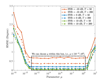
Figure 2: RMSE versus $\mu$, with $M=10$ sensors (4 of which fail), $K=2$ sources, $\lambda_{1}=2$, and $\lambda_{2}=0.2$.

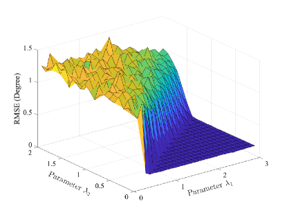
Figure 3: RMSE versus $\lambda_{1}$ and $\lambda_{2}$, with $M=10$ sensors (4 of which fail), $K=2$ sources, $T=100$ snapshots, $\text{SNR}=0~{}\text{dB}$, and $\mu=0.01$.

5.B CONVERGENCE SPEED

We compare the convergence speed of the IRLS with several existing methods, i.e., SVT, APG, and ADMM. Considering again a ULA of $M=10$ sensors, $4$ of which at random positions are distorted, receives $K=2$ signals from $-10^{\circ}$ and $10^{\circ}$. The objective function values of the algorithms versus the number of iterations are depicted in Fig. 4 with SNR $=0$ dB and $T=100$ snapshots. We see that the IRLS algorithm converges fastest in the sense that its objective function value decreases most rapidly, and it requires the least number of iterations to terminate, compared with the other three competitors.

The objective function value, CPU time and number of iterations are tabulated in Table 1 (upper) for SNR $=0$ dB and $T=100$ snapshots, and Table 1 (lower) for SNR $=0$ dB and $T=500$ snapshots. In both settings, the IRLS algorithm has the smallest objective function value, the least CPU time, and the least number of iterations, among all the examined algorithms.

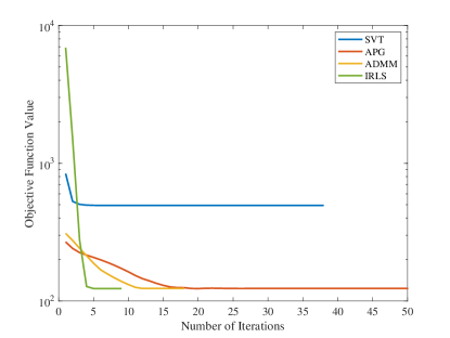
Figure 4: Objective function value versus number of iterations at $\text{SNR}=0~{}\text{dB}$ and $T=100$ snapshots.

Table 1: Comparison of objective function value, CPU time and number of iterations in two different settings.

$T=100$ snapshots, $\text{SNR}=0~{}\text{dB}$
Algorithm	$f({\bf Z},{\bf V})$	Time (sec)	No. Iter.
SVT [55]	493.8653	0.1205	5
APG [56]	123.3227	0.8403	22
ADMM [44]	123.3227	0.1029	13
IRLS	123.0227	0.0890	5

$T=500$ snapshots, $\text{SNR}=0~{}\text{dB}$
Algorithm	$f({\bf Z},{\bf V})$	Time (sec)	No. Iter.
SVT [55]	​​​1965.5994	0.6166	25
APG [56]	282.5776	4.3472	32
ADMM [44]	282.5776	5.8497	78
IRLS	282.2776	0.1063	10

5.C COMPUTATIONAL COMPLEXITY

We compare the computational complexity in this subsection. Note that the SVT, APG, and ADMM algorithms require one SVD of an $M\!\times\!T$ matrix per iteration, and the SVD consumes the most CPU time. As for the IRLS algorithm, the main calculation is to find the inverse of an $M\!\times\!M$ matrix per iteration. Their main computational cost is summarized in Table 2, where $K_{\text{svt}}$, $K_{\text{apg}}$, $K_{\text{admm}}$, and $K_{\text{irls}}$ denote the numbers of iterations for the SVT, APG, ADMM, and IRLS algorithms, respectively.

In Fig. 5, we plot the averaged CPU time against the number of snapshots at $M=10$ sensors (4 of which distorted), $K=2$ sources, SNR $=0$ dB, and $Q=1000$ Monte Carlo runs. It is seen that the CPU times of the SVT, APG, and ADMM algorithms are nearly linearly increasing with the number of snapshots. This is consistent with the theoretical analysis in Table 2. Fig. 6 displays the CPU time versus the number of sensors with $T=100$ snapshots and the other parameters are the same as those in Fig. 5. We see that the curves of the CPU time of the SVT, APG, and ADMM algorithms are approximately linearly correlated to the number of sensors in a log scale, which again matches the theoretical calculations in Table 2.

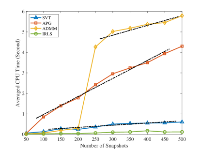
Figure 5: Computational complexity versus number of snapshots.

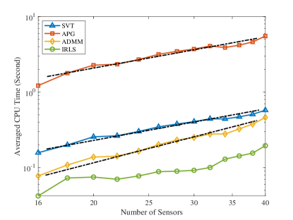
Figure 6: Computational complexity versus number of sensors.

Table 2: Computational complexity.

Algorithm	Complexity
SVT [55]	$K_{\text{svt}}\mathcal{O}(T\!M^{2})$
APG [56]	$K_{\text{apg}}\mathcal{O}(T\!M^{2})$
ADMM [44]	$K_{\text{admm}}\mathcal{O}(T\!M^{2})$
IRLS	$K_{\text{irls}}\mathcal{O}(M^{3})$

5.D DOA ESTIMATION PERFORMANCE

We use the RMSE and resolution probability as DOA estimation performance measures. The resolution probability is defined as

$$\text{ResProb}={N_{\text{succ}}}/{Q},$$

where as in the previous examples $Q$ is the number of Monte Carlo runs, and $N_{\text{succ}}$ denotes the number of trials where all the DOAs are successfully estimated. The trial is counted as a successful one if the following inequality is satisfied: $\max_{k}\{|\hat{\theta}_{k}-\theta_{k}|\}\leq 0.5^{\circ}$.

In the first example, we consider a ULA of $M=10$ sensors, $3$ of which at random positions are distorted, $K=2$ signals from $-10^{\circ}$ and $10^{\circ}$, $T=100$ snapshots, and $Q=5000$ Monte Carlo trials. The RMSE and resolution probability are depicted in Figs. 7 and 8, respectively. The traditional Cramér–Rao bound (CRB) with known sensor errors [63] is plotted as a benchmark. Note that the curve labelled as “MUSIC-Known” denotes the MUSIC method with exact knowledge of the distorted sensors. It is seen that the SVT and MUSIC have bad performance even when the SNR becomes large. The APG, ADMM, and IRLS algorithms perform well when the SNR increases, their RMSEs decrease and their resolution probabilities increase up to $1$. The IRLS algorithm outperforms the other two state-of-the-art methods, i.e., APG and ADMM.

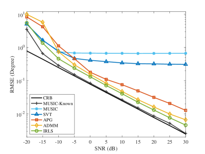
Figure 7: RMSE versus SNR.

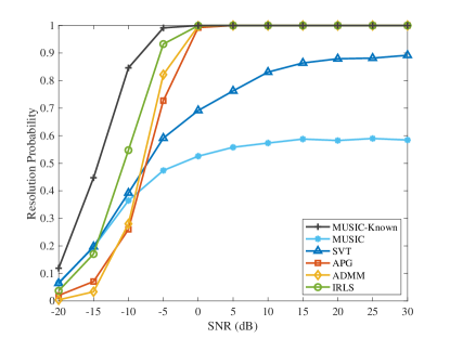
Figure 8: Resolution probability versus SNR.

In the next example, we examine the DOA estimation performance for different numbers of snapshots. The SNR is set to be $0$ dB, and the remaining parameters are the same as those of the former example. The RMSE and resolution probability of the methods are plotted in Figs. 9 and 10, respectively. The results demonstrate a better performance of the IRLS algorithm compared with the SVT, APG, and ADMM methods.

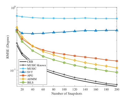
Figure 9: RMSE versus number of snapshots.

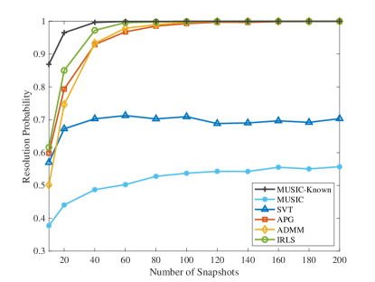
Figure 10: Resolution probability versus number of snapshots.

In the last example of this subsection, we evaluate the DOA estimation performance in view of the source separation angle. The settings of SNR $=0$ dB, $K=2$ sources, and $T=100$ snapshots are employed. The first signal is from $0^{\circ}$, while the DOA of the second signal changes from $1^{\circ}$ to $20^{\circ}$ with a stepsize of $1^{\circ}$. The other parameters are unchanged as those in the first example of this subsection. The RMSE and resolution probability versus angular separation are displayed in Figs. 11 and 12, respectively. These again indicate that the IRLS algorithm outperforms the SVT, APG, and ADMM algorithms in terms of RMSE and resolution probability.

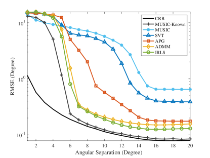
Figure 11: RMSE versus source separation angle.

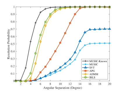
Figure 12: Resolution probability versus source separation angle.

5.E DISTORTED SENSOR DETECTION PERFORMANCE

Parallel to the three examples in Section 5.D, we now examine the performance of the detection of distorted sensors of the SVT, APG, ADMM, and IRLS algorithms. The threshold in Algorithm 3 is set as $h=10d$. We utilize the success detection rate as a metric, which is defined as

$$\text{DetecRate}={N_{\text{detec}}}/{Q}.$$

$N_{\text{detec}}$ denotes the number of trials where the number of distorted sensors is correctly estimated, and meanwhile their positions are exactly found. The results are given in Figs. 13, 14, and 15, which show that the ADMM is the best amongst all tested methods in terms of identifying the distorted sensors, followed by the IRLS algorithm.

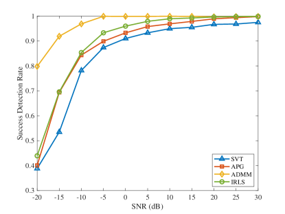
Figure 13: Success detection rate versus SNR.

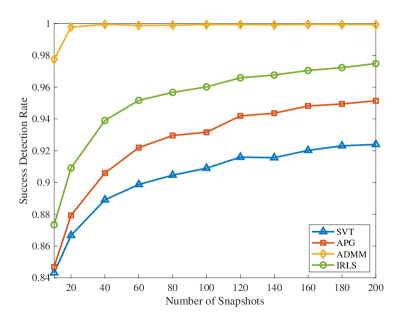
Figure 14: Success detection rate versus number of snapshots.

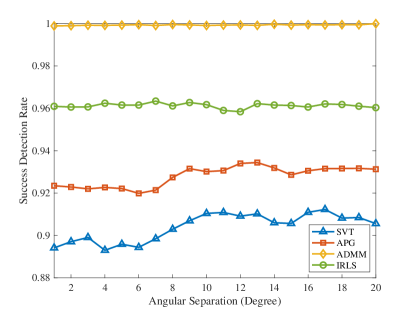
Figure 15: Success detection rate versus source separation angle.

6 CONCLUSION

We studied the problem of simultaneously estimating direction-of-arrival (DOA) of signals and detecting distorted sensors. It is assumed that the distorted sensors occur randomly, and the number of distorted sensors is much smaller than the total number of sensors. The problem was formulated via low-rank and row-sparse decomposition, and solved by iteratively reweighted least squares (IRLS). Both noiseless and noisy cases were considered. Theoretical analyses of algorithm convergence were provided. Computational cost of the IRLS algorithm was compared with that of several existing methods. Simulation results were conducted for parameter selection, convergence speed, computational time, and performance of DOA estimation as well as distorted sensor detection. The IRLS method was demonstrated to have higher DOA estimate accuracy and lower computational cost than other methods, and the alternating direction method of multipliers was shown to be slightly better than the IRLS algorithm in distorted sensor detection.

APPENDIX

6.A Proof of Theorem 1

We calculate the difference between the objective function values in two successive iterations as

$$f({\bf Z}_{k})-f({\bf Z}_{k+1})$$

$$=~{} \|[{\bf Z}_{k},\mu{\bf I}]\|_{*}-\|[{\bf Z}_{k+1},\mu{\bf I}]\|_{*}$$

$$+\lambda\left(\|[{\bf Y}-{\bf Z}_{k},\mu{\bf 1}]\|_{2,1}-\|[{\bf Y}-{\bf Z}_{k+1},\mu{\bf 1}]\|_{2,1}\right)$$

$$=~{} \text{trace}\!\left(\!\left({\bf Z}_{k}{\bf Z}_{k}^{\text{H}}+\mu^{2}{\bf I}\right)^{\frac{1}{2}}\!\right)-\text{trace}\!\left(\!\left({\bf Z}_{k+1}{\bf Z}_{k+1}^{\text{H}}+\mu^{2}{\bf I}\right)^{\frac{1}{2}}\!\right)$$

$$+\lambda\left(\|[{\bf Y}-{\bf Z}_{k},\mu{\bf 1}]\|_{2,1}-\|[{\bf Y}-{\bf Z}_{k+1},\mu{\bf 1}]\|_{2,1}\right)$$

$$\geq~{} \text{trace}\!\left(\frac{1}{2}\left({\bf Z}_{k}{\bf Z}_{k}^{\text{H}}-{\bf Z}_{k+1}{\bf Z}_{k+1}^{\text{H}}\right){\bf P}_{k}\!\right)$$

$$+\frac{\lambda}{2}\text{trace}\!\left({\bf Q}_{k}\left[\left({\bf Y}\!-\!{\bf Z}_{k}\right)\left({\bf Y}\!-\!{\bf Z}_{k}\right)^{\text{H}}\right.\right.$$

$$\qquad\qquad\quad\left.\left.-\left({\bf Y}\!-\!{\bf Z}_{k+1}\right)\left({\bf Y}\!-\!{\bf Z}_{k+1}\right)^{\text{H}}\right]\right)$$ (27)

$$=~{} \text{trace}\!\left(\frac{1}{2}({\bf Z}_{k}-{\bf Z}_{k+1})({\bf Z}_{k}-{\bf Z}_{k+1})^{\text{H}}{\bf P}_{k}\right)$$

$$+\text{trace}\!\left(({\bf Z}_{k}-{\bf Z}_{k+1}){\bf Z}_{k+1}^{\text{H}}{\bf P}_{k}\right)$$

$$+\frac{\lambda}{2}\text{trace}\!\left(2{\bf Q}_{k}{\bf Y}({\bf Z}_{k+1}-{\bf Z}_{k})^{\text{H}}\right)$$

$$+\frac{\lambda}{2}\text{trace}\!\left({\bf Q}_{k}({\bf Z}_{k}{\bf Z}_{k}^{\text{H}}-{\bf Z}_{k+1}{\bf Z}_{k+1}^{\text{H}})\right)$$

$$=~{} \text{trace}\!\left(\frac{1}{2}({\bf Z}_{k}-{\bf Z}_{k+1})({\bf Z}_{k}-{\bf Z}_{k+1})^{\text{H}}{\bf P}_{k}\right)$$

$$+\text{trace}\!\left(({\bf Z}_{k}-{\bf Z}_{k+1}){\bf Z}_{k+1}^{\text{H}}{\bf P}_{k}\right)$$

$$+\frac{\lambda}{2}\text{trace}\!\left(2{\bf Q}_{k}{\bf Y}({\bf Z}_{k+1}-{\bf Z}_{k})^{\text{H}}\right)$$

$$+\frac{\lambda}{2}\text{trace}\!\left({\bf Q}_{k}({\bf Z}_{k}-{\bf Z}_{k+1})({\bf Z}_{k}-{\bf Z}_{k+1})^{\text{H}}\right)$$

$$+\lambda~{}\!\text{trace}\!\left({\bf Q}_{k}({\bf Z}_{k}-{\bf Z}_{k+1}){\bf Z}_{k+1}^{\text{H}}\right)$$

$$\geq~{} \text{trace}\!\left(({\bf Z}_{k}-{\bf Z}_{k+1}){\bf Z}_{k+1}^{\text{H}}{\bf P}_{k}\right)$$

$$+\text{trace}\!\left(\lambda{\bf Q}_{k}{\bf Y}({\bf Z}_{k+1}-{\bf Z}_{k})^{\text{H}}\right)$$

$$+\text{trace}\!\left(\lambda{\bf Q}_{k}({\bf Z}_{k}-{\bf Z}_{k+1}){\bf Z}_{k+1}^{\text{H}}\right)$$ (28)

$$=~{} \text{trace}\!\left(({\bf Z}_{k}-{\bf Z}_{k+1}){\bf Z}_{k+1}^{\text{H}}({\bf P}_{k}+\lambda{\bf Q}_{k})\right)$$

$$+\text{trace}\!\left(\lambda{\bf Q}_{k}{\bf Y}({\bf Z}_{k+1}-{\bf Z}_{k})^{\text{H}}\right)$$

$$=~{} \text{trace}\!\left(({\bf P}_{k}+\lambda{\bf Q}_{k}){\bf Z}_{k+1}({\bf Z}_{k}-{\bf Z}_{k+1})^{\text{H}}\right)$$

$$+\text{trace}\!\left(\lambda{\bf Q}_{k}{\bf Y}({\bf Z}_{k+1}-{\bf Z}_{k})^{\text{H}}\right)$$

$$=~{} \text{trace}\!\left(\lambda{\bf Q}_{k}{\bf Y}({\bf Z}_{k}-{\bf Z}_{k+1})^{\text{H}}\right)$$

$$+\text{trace}\!\left(\lambda{\bf Q}_{k}{\bf Y}({\bf Z}_{k+1}-{\bf Z}_{k})^{\text{H}}\right)$$ (29)

$$=~{} 0,$$

which indicates that $f({\bf Z})$ is a non-increasing function with sequence $\{{\bf Z}_{k}\}$ generated by the IRLS procedure (13). The first equality is based on the definition of the objective function in (12), and the second equality uses $\|{\bf Z}\|_{*}=\text{trace}\left(\left({\bf Z}{\bf Z}^{\mathrm{H}}\right)^{-\frac{1}{2}}\right)$ when $M<T$. Inequality (6.A) holds thanks to Lemmata 1 and 2. Inequality (6.A) holds because of $\text{trace}\!\left(({\bf Z}_{k}-{\bf Z}_{k+1})({\bf Z}_{k}-{\bf Z}_{k+1})^{\text{H}}{\bf P}\right)\geq 0$ and $\text{trace}\!\left({\bf Q}({\bf Z}_{k}-{\bf Z}_{k+1})({\bf Z}_{k}-{\bf Z}_{k+1})^{\text{H}}\right)\geq 0$, which result from the fact that ${\bf P}$ and ${\bf Q}$ are symmetric matrices and $\text{trace}\!\left({\bf X}{\bf X}^{\text{H}}\right)=\|{\bf X}\|_{\text{F}}^{2}\geq 0$. Equality (6.A) holds true according to the KKT condition, i.e., $({\bf P}_{k}+\lambda{\bf Q}_{k}){\bf Z}_{k+1}=\lambda{\bf Q}_{k}{\bf Y}$.

Since $f({\bf Z})$ is a non-increasing, we have

$$\|{\bf Z}_{k}\|_{*} =\text{trace}\!\left(\left({\bf Z}{\bf Z}^{\mathrm{H}}\right)^{-\frac{1}{2}}\right)<\text{trace}\!\left(\left({\bf Z}{\bf Z}^{\mathrm{H}}+\mu^{2}{\bf I}\right)^{-\frac{1}{2}}\right)$$

$$=\|[{\bf Z}_{k},\mu{\bf I}]\|_{*}\leq f({\bf Z}_{k})\leq f({\bf Z}_{0}),$$

which indicates that the sequence $\{{\bf Z}_{k}\}$ is bounded in terms of its nuclear norm.

Besides, combining (13) and (6.A) yields

$$f({\bf Z}_{k})-f({\bf Z}_{k+1})$$

$$\geq~{} \text{trace}\!\left(\frac{1}{2}\left({\bf Z}_{k}{\bf Z}_{k}^{\text{H}}-{\bf Z}_{k+1}{\bf Z}_{k+1}^{\text{H}}\right){\bf P}_{k}\!\right)$$

$$+\frac{\lambda}{2}\text{trace}\!\left({\bf Q}_{k}\left[\left({\bf Y}\!-\!{\bf Z}_{k}\right)\left({\bf Y}\!-\!{\bf Z}_{k}\right)^{\text{H}}\right.\right.$$

$$\qquad\qquad\quad\left.\left.-\left({\bf Y}\!-\!{\bf Z}_{k+1}\right)\left({\bf Y}\!-\!{\bf Z}_{k+1}\right)^{\text{H}}\right]\right)$$

$$=~{} \frac{1}{2}\text{trace}\!\left(({\bf P}_{k}+\lambda{\bf Q}_{k})({\bf Z}_{k}-{\bf Z}_{k+1})({\bf Z}_{k}-{\bf Z}_{k+1})^{\mathrm{H}}\right)$$

$$\geq~{} \frac{1}{2}\!\!\sum_{i=1}^{M}\!\zeta_{i}\!({\bf P}_{k}\!\!+\!\!\lambda{\bf Q}_{k})\zeta_{M\!-i+1}\!(\!({\bf Z}_{k}\!\!-\!\!{\bf Z}_{k\!+\!1})\!({\bf Z}_{k}\!\!-\!\!{\bf Z}_{k\!+\!1})^{\!\mathrm{H}}\!)$$ (30)

$$\geq~{} \frac{1}{2}\zeta_{M}\!({\bf P}_{k}\!\!+\!\!\lambda{\bf Q}_{k})\|{\bf Z}_{k}\!-\!{\bf Z}_{k\!+\!1}\|_{\mathrm{F}}^{2}\geq\frac{1}{2}\zeta_{\mathrm{min}}\!\times\!\|{\bf Z}_{k}\!-\!{\bf Z}_{k\!+\!1}\|_{\mathrm{F}}^{2},$$

where $\zeta_{i}(\cdot)$ denotes the $i$th largest eigenvalue of its input Hermitian matrix, inequality (30) follows from the fact that $\text{trace}({\bf X}{\bf Y})\geq\sum_{i=1}^{M}\zeta_{i}({\bf X})\zeta_{M-i+1}({\bf Y})$ holds for any two positive semi-definite matrices ${\bf X}$ and ${\bf Y}\in\mathbb{C}^{M\times M}$ [49], and in the last inequality, we have defined $\zeta_{\mathrm{min}}>0$ as the smallest eigenvalue of ${\bf P}_{k}\!+\!\lambda{\bf Q}_{k}$ over all $k$. Summing all the above inequalities for all $k\geq 0$, we have

$$f({\bf Z}_{0})\geq\frac{1}{2}\zeta_{\mathrm{min}}\sum_{k=0}^{\infty}\|{\bf Z}_{k}-{\bf Z}_{k+1}\|_{\mathrm{F}}^{2},$$

which implies that $\lim_{k\to\infty}\|{\bf Z}_{k}-{\bf Z}_{k+1}\|_{\mathrm{F}}=0$.

6.B Proof of Theorem 2

For any matrices ${\bf Y}$ and ${\bf Z}$ $\in\mathbb{C}^{M\times T}$, we have

$$\|[{\bf Y}\!-\!{\bf Z},\mu{\bf 1}]\|_{2,1}=~{} \sum_{i=1}^{M}\sqrt{\|({\bf Y}\!-\!{\bf Z})_{i,:}\|_{2}^{2}+\mu^{2}}$$

$$\geq~{} \sum_{i=1}^{M}|\mu|~{}=~{}|\mu|M$$

$$\|[{\bf Z},\mu{\bf I}]\|_{*}=~{} \text{trace}\!\left(\left({\bf Z}{\bf Z}^{\text{H}}+\mu^{2}{\bf I}\right)^{\frac{1}{2}}\right)$$

$$\geq~{} \left(\text{trace}\!\left({\bf Z}{\bf Z}^{\text{H}}+\mu^{2}{\bf I}\right)\right)^{\frac{1}{2}}$$ (31)

$$=~{} \left(\text{trace}\!\left({\bf Z}{\bf Z}^{\text{H}}\right)+M\mu^{2}\right)^{\frac{1}{2}}$$

$$\geq~{} \left(M\mu^{2}\right)^{\frac{1}{2}}~{}=~{}|\mu|\sqrt{M}.$$

Inequality (31) holds because $\text{trace}\!\left({\bf X}^{\frac{1}{2}}\right)\!=\!\sum_{i}\!\sqrt{\zeta_{i}}\geq\sqrt{\sum_{i}\zeta_{i}}=\left(\text{trace}\!\left({\bf X}\right)\right)^{\frac{1}{2}}$ for any symmetric matrix ${\bf X}$, with $\zeta_{i}$ being the eigenvalue of ${\bf X}$. Therefore, the objective function in (12) is bounded below as $f({\bf Z})=\|[{\bf Z},\mu{\bf I}]\|_{*}+\lambda\|[{\bf Y}\!-\!{\bf Z},\mu{\bf 1}]\|_{2,1}\geq|\mu|(\sqrt{M}+\lambda M)$.

6.C Proof of Theorem 3

Denote the limit point of sequence $\{{\bf Z}_{k}\}$ as ${\bf Z}_{k+1}$. Then, according to $\lim_{k\to\infty}\|{\bf Z}_{k}-{\bf Z}_{k+1}\|_{\mathrm{F}}=0$ in Theorem 1 and (13), we have ${\bf Z}_{k+1}=\lambda({\bf P}_{k+1}+\lambda{\bf Q}_{k+1})^{-1}{\bf Q}_{k+1}{\bf Y}$, that is, ${\bf P}_{k+1}{\bf Z}_{k+1}+\lambda{\bf Q}_{k+1}({\bf Z}_{k+1}-{\bf Y})={\bf 0}$. This indicates that ${\bf Z}_{k+1}$ satisfies the KKT condition. Since Problem (12) is convex w.r.t. ${\bf Z}$, the stationary point is globally optimal.

6.D Proof of Theorem 4

Similar to the proof of Theorem 1, we calculate the difference between the objective function values in two successive iterations as

$$f({\bf Z}_{k},{\bf V}_{k})-f({\bf Z}_{k+1},{\bf V}_{k+1})$$

$$=~{} \frac{1}{2}\|{\bf Y}\!-\!{\bf Z}_{k}\!-\!{\bf V}_{k}\|_{\text{F}}^{2}-\!\frac{1}{2}\|{\bf Y}\!-\!{\bf Z}_{k+1}\!-\!{\bf V}_{k+1}\|_{\text{F}}^{2}$$

$$+\lambda_{1}\|[{\bf Z}_{k},\mu{\bf I}]\|_{*}-\lambda_{1}\|[{\bf Z}_{k+1},\mu{\bf I}]\|_{*}$$

$$+\lambda_{2}\|[{\bf V}_{k},\mu{\bf 1}]\|_{2,1}-\lambda_{2}\|[{\bf V}_{k+1},\mu{\bf 1}]\|_{2,1}$$

$$\geq~{} \frac{1}{2}\|{\bf Y}\!-\!{\bf Z}_{k}\!-\!{\bf V}_{k}\|_{\text{F}}^{2}-\!\frac{1}{2}\|{\bf Y}\!-\!{\bf Z}_{k+1}\!-\!{\bf V}_{k+1}\|_{\text{F}}^{2}$$

$$+\lambda_{1}~{}\!\text{trace}\!\left(\frac{1}{2}\left({\bf Z}_{k}{\bf Z}_{k}^{\text{H}}-{\bf Z}_{k+1}{\bf Z}_{k+1}^{\text{H}}\right){\bf P}_{k}\right)$$

$$+\frac{\lambda_{2}}{2}\text{trace}\!\left({\bf Q}_{k}\left({\bf V}_{k}{\bf V}_{k}^{\text{H}}-{\bf V}_{k+1}{\bf V}_{k+1}^{\text{H}}\right)\right)$$

$$=~{} \frac{1}{2}\|{\bf Y}\!-\!{\bf Z}_{k}\!-\!{\bf V}_{k}\|_{\text{F}}^{2}-\!\frac{1}{2}\|{\bf Y}\!-\!{\bf Z}_{k+1}\!-\!{\bf V}_{k+1}\|_{\text{F}}^{2}$$

$$+\lambda_{1}~{}\!\text{trace}\!\left(\frac{1}{2}\left({\bf Z}_{k}-{\bf Z}_{k+1}\right)\left({\bf Z}_{k}-{\bf Z}_{k+1}\right)^{\text{H}}{\bf P}_{k}\right)$$

$$+\lambda_{1}~{}\!\text{trace}\!\left(\left({\bf Z}_{k}-{\bf Z}_{k+1}\right){\bf Z}_{k+1}^{\text{H}}{\bf P}_{k}\right)$$

$$+\frac{\lambda_{2}}{2}\text{trace}\!\left({\bf Q}_{k}\left({\bf V}_{k}-{\bf V}_{k+1}\right)\left({\bf V}_{k}-{\bf V}_{k+1}\right)^{\text{H}}\right)$$

$$+\lambda_{2}~{}\!\text{trace}\!\left({\bf Q}_{k}({\bf V}_{k}-{\bf V}_{k+1}){\bf V}_{k+1}^{\text{H}}\right)$$ (32)

$$\geq~{} \frac{1}{2}\text{trace}\!\left(({\bf Z}_{k}-{\bf Z}_{k+1})({\bf Z}_{k}-{\bf Z}_{k+1})^{\text{H}}\right.$$

$$\qquad\quad\left.+~{}({\bf V}_{k}-{\bf V}_{k+1})({\bf V}_{k}-{\bf V}_{k+1})^{\text{H}}\right)$$

$$+\text{trace}\!\left((-{\bf Y}+{\bf Z}_{k+1})({\bf Z}_{k}-{\bf Z}_{k+1})^{\text{H}}\right.$$

$$\qquad\quad\left.+~{}(-{\bf Y}+{\bf V}_{k+1})({\bf V}_{k}-{\bf V}_{k+1})^{\text{H}}\right.$$

$$\qquad\quad\left.+~{}{\bf Z}_{k}{\bf V}_{k}^{\text{H}}-{\bf Z}_{k+1}{\bf V}_{k+1}^{\text{H}}\right)$$

$$+\lambda_{1}~{}\!\text{trace}\!\left(\left({\bf Z}_{k}-{\bf Z}_{k+1}\right){\bf Z}_{k+1}^{\text{H}}{\bf P}_{k}\right)$$

$$+\lambda_{2}~{}\!\text{trace}\!\left({\bf Q}_{k}({\bf V}_{k}-{\bf V}_{k+1}){\bf V}_{k+1}^{\text{H}}\right)$$

$$=~{} \frac{1}{2}\text{trace}\!\left(({\bf Z}_{k}-{\bf Z}_{k+1})({\bf Z}_{k}-{\bf Z}_{k+1})^{\text{H}}\right.$$

$$\qquad\quad\left.+~{}({\bf V}_{k}-{\bf V}_{k+1})({\bf V}_{k}-{\bf V}_{k+1})^{\text{H}}\right)$$

$$+\text{trace}\!\left({\bf Z}_{k}{\bf V}_{k}^{\text{H}}-{\bf Z}_{k+1}{\bf V}_{k+1}^{\text{H}}\right)$$

$$+\text{trace}\!\left(-{\bf V}_{k}({\bf Z}_{k}-{\bf Z}_{k+1})^{\text{H}}\right)$$

$$+\text{trace}\!\left(-{\bf Z}_{k}({\bf V}_{k}-{\bf V}_{k+1})^{\text{H}}\right)$$

$$=~{} \frac{1}{2}\text{trace}\!\left(({\bf Z}_{k}-{\bf Z}_{k+1})({\bf Z}_{k}-{\bf Z}_{k+1})^{\text{H}}\right.$$

$$\qquad\quad\left.+~{}({\bf V}_{k}-{\bf V}_{k+1})({\bf V}_{k}-{\bf V}_{k+1})^{\text{H}}\right)$$

$$+\text{trace}\!\left(({\bf Z}_{k}-{\bf Z}_{k+1})({\bf V}_{k+1}-{\bf V}_{k})^{\text{H}}\right)$$

$$=~{} \frac{1}{2}\text{trace}\!\left(({\bf Z}_{k}-{\bf Z}_{k+1}-{\bf V}_{k}+{\bf V}_{k+1})\cdot\right.$$

$$\qquad\quad\left.({\bf Z}_{k}-{\bf Z}_{k+1}-{\bf V}_{k}+{\bf V}_{k+1})^{\text{H}}\right)$$

$$=~{} \frac{1}{2}\|{\bf Z}_{k}-{\bf Z}_{k+1}-{\bf V}_{k}+{\bf V}_{k+1}\|_{\text{F}}^{2}~{}\geq~{}0,$$

which indicates that $f({\bf Z},{\bf V})$ is a non-increasing function. Since $f({\bf Z},{\bf V})$ is non-increasing, we have

$$\min\{\lambda_{1},\lambda_{2}\}\left(\|[{\bf Z}_{k},\mu{\bf I}]\|_{*}+\|[{\bf V}_{k},\mu{\bf 1}]\|_{2,1}\right)$$

$$\leq~{} \lambda_{1}\|[{\bf Z}_{k},\mu{\bf I}]\|_{*}+\lambda_{2}\|[{\bf V}_{k},\mu{\bf 1}]\|_{2,1}$$

$$\leq~{} f({\bf Z}_{k},{\bf V}_{k})~{}\leq~{}f({\bf Z}_{0},{\bf V}_{0}).$$

Hence, $\|{\bf Z}_{k}\|_{*}+\|{\bf V}_{k}\|_{2,1}<\|[{\bf Z}_{k},\mu{\bf I}]\|_{*}+\|[{\bf V}_{k},\mu{\bf 1}]\|_{2,1}\leq\frac{f({\bf Z}_{0},{\bf V}_{0})}{\min\{\lambda_{1},\lambda_{2}\}}$, which indicates that the sequence $\{({\bf Z}_{k},{\bf V}_{k})\}$ is bounded.

Besides, combining (26) and (32) yields

$$f({\bf Z}_{k},{\bf V}_{k})-f({\bf Z}_{k+1},{\bf V}_{k+1})$$

$$\geq~{} \frac{\lambda_{1}}{2}~{}\!\text{trace}\!\left(\left({\bf Z}_{k}-{\bf Z}_{k+1}\right)\left({\bf Z}_{k}-{\bf Z}_{k+1}\right)^{\text{H}}{\bf P}_{k}\right)$$

$$+\frac{\lambda_{2}}{2}\text{trace}\!\left({\bf Q}_{k}\left({\bf V}_{k}-{\bf V}_{k+1}\right)\left({\bf V}_{k}-{\bf V}_{k+1}\right)^{\text{H}}\right)$$

$$+\frac{1}{2}\text{trace}\!\left(({\bf Z}_{k}-{\bf Z}_{k+1})({\bf Z}_{k}-{\bf Z}_{k+1})^{\mathrm{H}}\right)$$

$$\geq~{} \frac{\lambda_{1}}{2}~{}\!\text{trace}\!\left(\left({\bf Z}_{k}-{\bf Z}_{k+1}\right)\left({\bf Z}_{k}-{\bf Z}_{k+1}\right)^{\text{H}}{\bf P}_{k}\right)$$

$$+\frac{\lambda_{2}}{2}\text{trace}\!\left({\bf Q}_{k}\left({\bf V}_{k}-{\bf V}_{k+1}\right)\left({\bf V}_{k}-{\bf V}_{k+1}\right)^{\text{H}}\right)$$

$$\geq~{} \frac{\lambda_{1}}{2}\sum_{i}^{M}\zeta_{i}({\bf P}_{k})\zeta_{M-i+1}(({\bf Z}_{k}\!-\!{\bf Z}_{k+1})({\bf Z}_{k}\!-\!{\bf Z}_{k+1})^{\mathrm{H}})$$

$$+\frac{\lambda_{2}}{2}\sum_{i}^{M}\!\zeta_{i}({\bf Q}_{k})\zeta_{M\!-i+1}\!(\!(\!{\bf V}_{k}\!-\!{\bf V}_{k+1}\!)(\!{\bf V}_{k}\!-\!{\bf V}_{k+1}\!)^{\mathrm{H}}\!)$$

$$\geq~{} \frac{\lambda_{1}}{2}\zeta_{\mathrm{min}}^{({\bf P})}\times\|{\bf Z}_{k}\!-\!{\bf Z}_{k+1}\|_{\mathrm{F}}^{2}+\frac{\lambda_{1}}{2}\zeta_{\mathrm{min}}^{({\bf Q})}\times\|{\bf V}_{k}\!-\!{\bf V}_{k+1}\|_{\mathrm{F}}^{2},$$

where $\zeta_{\mathrm{min}}^{({\bf P})}$ and $\zeta_{\mathrm{min}}^{({\bf Q})}$ are the smallest eigenvalues of ${\bf P}_{k}$ and ${\bf Q}_{k}$, respectively, over all $k$. Summing all the above inequalities for all $k\geq 0$, we have

$$f({\bf Z}_{0},{\bf V}_{0})\geq ~{}\frac{\lambda_{1}}{2}\zeta_{\mathrm{min}}^{({\bf P})}\sum_{k=0}^{\infty}\|{\bf Z}_{k}-{\bf Z}_{k+1}\|_{\mathrm{F}}^{2}$$

$$+\frac{\lambda_{2}}{2}\zeta_{\mathrm{min}}^{({\bf Q})}\sum_{k=0}^{\infty}\|{\bf V}_{k}-{\bf V}_{k+1}\|_{\mathrm{F}}^{2},$$

which implies that $\lim_{k\to\infty}\|{\bf Z}_{k}-{\bf Z}_{k+1}\|_{\mathrm{F}}=0$ and $\lim_{k\to\infty}\|{\bf V}_{k}-{\bf V}_{k+1}\|_{\mathrm{F}}=0$.

6.E Proof of Theorem 5

Considering $\|{\bf Y}-{\bf Z}-{\bf V}\|_{\text{F}}^{2}\geq 0$ and the inequalities in Appendix 6.B, we can prove that the objective function in (19) is bounded below as $f({\bf Z},{\bf V})=\frac{1}{2}\|{\bf Y}\!-\!{\bf Z}\!-\!{\bf V}\|_{\text{F}}^{2}+\lambda_{1}\|[{\bf Z},\mu{\bf I}]\|_{*}+\lambda_{2}\|[{\bf V},\mu{\bf 1}]\|_{2,1}\geq|\mu|(\lambda_{1}\sqrt{M}+\lambda_{2}M)$.

6.F Proof of Theorem 6

Denote the limit point of the sequence $\{({\bf Z}_{k},{\bf V}_{k})\}$ as $({\bf Z}_{k+1},{\bf V}_{k+1})$. Then, according to $\lim_{k\to\infty}\|{\bf Z}_{k}-{\bf Z}_{k+1}\|_{\mathrm{F}}=0$ and $\lim_{k\to\infty}\|{\bf V}_{k}-{\bf V}_{k+1}\|_{\mathrm{F}}=0$ in Theorem 4 and (26), we have

$$\left\{\!\!\begin{array}[]{l}{\bf Z}_{k+1}=({\bf I}+\lambda_{1}{\bf P}_{k+1})^{-1}({\bf Y}-{\bf V}_{k+1})\\ {\bf V}_{k+1}\!=({\bf I}+\lambda_{2}{\bf Q}_{k+1})^{-1}({\bf Y}-{\bf Z}_{k+1}),\end{array}\right.$$

which is the KKT condition of Problem (19). Since Problem (19) is convex w.r.t. ${\bf Z}$ and ${\bf V}$, the stationary point is globally optimal.

References

- [1] H. Krim and M. Viberg, “Two decades of array signal processing research: The parametric approach,” IEEE Signal Processing Magazine, vol. 13, no. 4, pp. 67–94, July 1996.
- [2] H. L. Van Trees, “Chapter 1 - Introduction,” in Optimum Array Processing. John Wiley & Sons, Ltd, 2002, pp. 1–16.
- [3] M. Viberg, “Chapter 11 - Introduction to array processing,” in Academic Press Library in Signal Processing: Volume 3, A. M. Zoubir, M. Viberg, R. Chellappa, and S. Theodoridis, Eds. Elsevier, 2014, vol. 3, pp. 463–502.
- [4] R. Schmidt, “Multiple emitter location and signal parameter estimation,” IEEE Transactions on Antennas and Propagation, vol. 34, no. 3, pp. 276–280, March 1986.
- [5] R. Roy and T. Kailath, “ESPRIT-estimation of signal parameters via rotational invariance techniques,” IEEE Transactions on Acoustics, Speech, and Signal Processing, vol. 37, no. 7, pp. 984–995, July 1989.
- [6] J. F. Böhme, “Estimation of spectral parameters of correlated signals in wavefields,” Signal Processing, vol. 11, no. 4, pp. 329–337, December 1986.
- [7] I. Ziskind and M. Wax, “Maximum likelihood localization of multiple sources by alternating projection,” IEEE Transactions on Acoustics, Speech, and Signal Processing, vol. 36, no. 10, pp. 1553–1560, October 1988.
- [8] S. Vorobyov, A. B. Gershman, Z.-Q. Luo, and N. Ma, “Adaptive beamforming with joint robustness against signal steering vector errors and interference nonstationarity,” in Proceedings of IEEE International Conference on Acoustics, Speech, and Signal Processing (ICASSP), vol. 5, Hong Kong, China, April 2003, pp. 345–348.
- [9] B. Wang, Y. D. Zhang, and W. Wang, “Robust DOA estimation in the presence of miscalibrated sensors,” IEEE Signal Processing Letters, vol. 24, no. 7, pp. 1073–1077, July 2017.
- [10] Q. Wang, T. Dou, H. Chen, W. Yan, and W. Liu, “Effective block sparse representation algorithm for DOA estimation with unknown mutual coupling,” IEEE Communications Letters, vol. 21, no. 12, pp. 2622–2625, December 2017.
- [11] Z. Yang, R. C. de Lamare, and W. Liu, “Sparsity-based STAP using alternating direction method with gain/phase errors,” IEEE Transactions on Aerospace and Electronic Systems, vol. 53, no. 6, pp. 2756–2768, December 2017.
- [12] K. N. Ramamohan, S. P. Chepuri, D. F. Comesaña, G. C. Pousa, and G. Leus, “Blind calibration for acoustic vector sensor arrays,” in Proceedings of IEEE International Conference on Acoustics, Speech and Signal Processing (ICASSP), Calgary, Canada, April 2018, pp. 3544–3548.
- [13] H. Huang, M. Fauß, and A. M. Zoubir, “Block sparsity-based DOA estimation with sensor gain and phase uncertainties,” in Proceedings of European Signal Processing Conference (EUSIPCO), A Coruna, Spain, September 2019, pp. 1–5.
- [14] B. Lin, J. Liu, M. Xie, and J. Zhu, “Direction-of-arrival tracking via low-rank plus sparse matrix decomposition,” IEEE Antennas and Wireless Propagation Letters, vol. 14, pp. 1302–1305, February 2015.
- [15] A. Das, “A Bayesian sparse-plus-low-rank matrix decomposition method for direction-of-arrival tracking,” IEEE Sensors Journal, vol. 17, no. 15, pp. 4894–4902, August 2017.
- [16] P. P. Markopoulos, N. Tsagkarakis, D. A. Pados, and G. N. Karystinos, “Direction finding with L1-norm subspaces,” in Compressive Sensing III, F. Ahmad, Ed., vol. 9109, International Society for Optics and Photonics. SPIE, May 2014, pp. 130–140.
- [17] P. P. Markopoulos, N. Tsagkarakis, D. A. Pados, and G. N. Karystinos, “Realified L1-PCA for direction-of-arrival estimation: Theory and algorithms,” EURASIP Journal on Advances in Signal Processing, vol. 30, pp. 1–16, June 2019.
- [18] B.-K. Yeo and Y. Lu, “Array failure correction with a genetic algorithm,” IEEE Transactions on Antennas and Propagation, vol. 47, no. 5, pp. 823–828, May 1999.
- [19] S. Vigneshwaran, N. Sundararajan, and P. Saratchandran, “Direction of arrival (DoA) estimation under array sensor failures using a minimal resource allocation neural network,” IEEE Transactions on Antennas and Propagation, vol. 55, no. 2, pp. 334–343, February 2007.
- [20] M. Muma, Y. Cheng, F. Roemer, M. Haardt, and A. M. Zoubir, “Robust source number enumeration for R-dimensional arrays in case of brief sensor failures,” in Proceedings of IEEE International Conference on Acoustics, Speech and Signal Processing (ICASSP), Kyoto, Japan, March 2012, pp. 3709–3712.
- [21] G. Oliveri, P. Rocca, and A. Massa, “Reliable diagnosis of large linear arrays-A Bayesian compressive sensing approach,” IEEE Transactions on Antennas and Propagation, vol. 60, no. 10, pp. 4627–4636, October 2012.
- [22] C. Zhu, W.-Q. Wang, H. Chen, and H. C. So, “Impaired sensor diagnosis, beamforming, and DOA estimation with difference co-array processing,” IEEE Sensors Journal, vol. 15, no. 7, pp. 3773–3780, July 2015.
- [23] M. Wang, Z. Zhang, and A. Nehorai, “Direction finding using sparse linear arrays with missing data,” in Proceedings of IEEE International Conference on Acoustics, Speech and Signal Processing (ICASSP), New Orleans, USA, March 2017, pp. 3066–3070.
- [24] C.-L. Liu and P. P. Vaidyanathan, “Robustness of difference coarrays of sparse arrays to sensor failures-Part I: A theory motivated by coarray MUSIC,” IEEE Transactions on Signal Processing, vol. 67, no. 12, pp. 3213–3226, June 2019.
- [25] P. Stoica, M. Viberg, K. M. Wong, and Q. Wu, “Maximum-likelihood bearing estimation with partly calibrated arrays in spatially correlated noise fields,” IEEE Transactions on Signal Processing, vol. 44, no. 4, pp. 888–899, April 1996.
- [26] B. Ng, J. P. Lie, M. Er, and A. Feng, “A practical simple geometry and gain/phase calibration technique for antenna array processing,” IEEE Transactions on Antennas and Propagation, vol. 57, no. 7, pp. 1963–1972, July 2009.
- [27] J. Jiang, F. Duan, J. Chen, Z. Chao, Z. Chang, and X. Hua, “Two new estimation algorithms for sensor gain and phase errors based on different data models,” IEEE Sensors Journal, vol. 13, no. 5, pp. 1921–1930, May 2013.
- [28] M. Pesavento, A. B. Gershman, and K. M. Wong, “Direction finding in partly calibrated sensor arrays composed of multiple subarrays,” IEEE Transactions on Signal Processing, vol. 50, no. 9, pp. 2103–2115, September 2002.
- [29] C. M. S. See and A. B. Gershman, “Direction-of-arrival estimation in partly calibrated subarray-based sensor arrays,” IEEE Transactions on Signal Processing, vol. 52, no. 2, pp. 329–338, February 2004.
- [30] B. Liao and S. C. Chan, “Direction finding with partly calibrated uniform linear arrays,” IEEE Transactions on Antennas and Propagation, vol. 60, no. 2, pp. 922–929, February 2012.
- [31] C. Steffens, P. Parvazi, and M. Pesavento, “Direction finding and array calibration based on sparse reconstruction in partly calibrated arrays,” in Proceedings of IEEE Sensor Array and Multichannel Signal Processing Workshop (SAM), A Coruna, Spain, June 2014, pp. 21–24.
- [32] B. Liao and S. C. Chan, “A review on direction finding in partly calibrated arrays,” in Proceedings of International Conference on Digital Signal Processing (DSP), Hong Kong, China, August 2014, pp. 812–816.
- [33] W. Suleiman, P. Parvazi, M. Pesavento, and A. M. Zoubir, “Non-coherent direction-of-arrival estimation using partly calibrated arrays,” IEEE Transactions on Signal Processing, vol. 66, no. 21, pp. 5776–5788, November 2018.
- [34] F. Afkhaminia and M. Azghani, “Sparsity-based direction of arrival estimation in the presence of gain/phase uncertainty,” in Proceedings of European Signal Processing Conference (EUSIPCO), Kos, Greece, September 2017, pp. 2616–2619.
- [35] G. C. F. Lee, A. S. Rawat, and G. W. Wornell, “Robust direction of arrival estimation in the presence of array faults using snapshot diversity,” in Proceedings of IEEE Global Conference on Signal and Information Processing (GlobalSIP), Ottawa, Canada, November 2019, pp. 1–5.
- [36] H. Huang and A. M. Zoubir, “Low-rank and sparse decomposition for joint DOA estimation and contaminated sensors detection with sparsely contaminated arrays,” in Proceedings of IEEE International Conference on Acoustics, Speech and Signal Processing (ICASSP), Toronto, Canada, June 2021, pp. 4615–4619.
- [37] J. H. Holland, “Reproductive plans and genetic operators,” in Adaptation in Natural and Artificial Systems: An Introductory Analysis with Applications to Biology, Control, and Artificial Intelligence. MIT Press, 1992, pp. 89–120.
- [38] N. Vaswani, T. Bouwmans, S. Javed, and P. Narayanamurthy, “Robust subspace learning: Robust PCA, robust subspace tracking, and robust subspace recovery,” IEEE Signal Processing Magazine, vol. 35, no. 4, pp. 32–55, July 2018.
- [39] N. Vaswani, Y. Chi, and T. Bouwmans, “Rethinking PCA for modern data sets: Theory, algorithms, and applications,” Proceedings of the IEEE, vol. 106, no. 8, pp. 1274–1276, August 2018.
- [40] T. Bouwmans, S. Javed, H. Zhang, Z. Lin, and R. Otazo, “On the applications of robust PCA in image and video processing,” Proceedings of the IEEE, vol. 106, no. 8, pp. 1427–1457, August 2018.
- [41] I. T. Jolliffe, “Outlier detection, influential observations and robust estimation of principal components,” in Principal Component Analysis. Springer New York, 1986, pp. 173–198.
- [42] J. Wright, Y. Peng, Y. Ma, A. Ganesh, and S. Rao, “Robust principal component analysis: Exact recovery of corrupted low-rank matrices by convex optimization,” in Proceedings of International Conference on Neural Information Processing Systems (NIPS), Red Hook, USA, December 2009, pp. 2080–2088.
- [43] C. Zhang, J. Liu, Q. Tian, C. Xu, H. Lu, and S. Ma, “Image classification by non-negative sparse coding, low-rank and sparse decomposition,” in Proceedings of Conference on Computer Vision and Pattern Recognition (CVPR), Colorado Spring, USA, August 2011, pp. 1673–1680.
- [44] Z. Lin, M. Chen, and Y. Ma, “The augmented Lagrange multiplier method for exact recovery of corrupted low-rank matrices,” 2010. [Online]. Available: https://arxiv.org/abs/1009.5055
- [45] Y. Bando, K. Itoyama, M. Konyo, S. Tadokoro, K. Nakadai, K. Yoshii, T. Kawahara, and H. G. Okuno, “Speech enhancement based on Bayesian low-rank and sparse decomposition of multichannel magnitude spectrograms,” IEEE/ACM Transactions on Audio, Speech, and Language Processing, vol. 26, no. 2, pp. 215–230, February 2018.
- [46] H. Xu, C. Caramanis, and S. Sanghavi, “Robust PCA via outlier pursuit,” IEEE Transactions on Information Theory, vol. 58, no. 5, pp. 3047–3064, May 2012.
- [47] G. Liu, Z. Lin, and Y. Yu, “Robust subspace segmentation by low-rank representation,” in Proceedings of International Conference on Machine Learning (ICML), Madison, USA, June 2010, pp. 663–670.
- [48] G. Liu, Z. Lin, S. Yan, J. Sun, Y. Yu, and Y. Ma, “Robust recovery of subspace structures by low-rank representation,” IEEE Transactions on Pattern Analysis and Machine Intelligence, vol. 35, no. 1, pp. 171–184, January 2013.
- [49] C. Lu, Z. Lin, and S. Yan, “Smoothed low rank and sparse matrix recovery by iteratively reweighted least squares minimization,” IEEE Transactions on Image Processing, vol. 24, no. 2, pp. 646–654, February 2015.
- [50] Q. Liu, Y. Gu, and H. C. So, “DOA estimation in impulsive noise via low-rank matrix approximation and weakly convex optimization,” IEEE Transactions on Aerospace and Electronic Systems, vol. 55, no. 6, pp. 3603–3616, December 2019.
- [51] H. Zhang, Z. Lin, C. Zhang, and E. Chang, “Exact recoverability of robust PCA via outlier pursuit with tight recovery bounds,” in Proceedings of the AAAI Conference on Artificial Intelligence, vol. 29, no. 1, Austin, USA, February 2015.
- [52] X. Li, J. Ren, S. Rambhatla, Y. Xu, and J. Haupt, “Robust PCA via dictionary based outlier pursuit,” in Proceedings of IEEE International Conference on Acoustics, Speech and Signal Processing (ICASSP), Calgary, Canada, April 2018, pp. 4699–4703.
- [53] C. Guyon, T. Bouwmans, and E.-H. Zahzah, “Foreground detection via robust low rank matrix factorization including spatial constraint with iterative reweighted regression,” in Proceedings of the International Conference on Pattern Recognition (ICPR), Tsukuba, Japan, November 2012, pp. 2805–2808.
- [54] P. Rodrêguez and B. Wohlberg, “Performance comparison of iterative reweighting methods for total variation regularization,” in Proceedings of IEEE International Conference on Image Processing (ICIP), Paris, France, October 2014, pp. 1758–1762.
- [55] J.-F. Cai, E. J. Candès, and Z. Shen, “A singular value thresholding algorithm for matrix completion,” SIAM Journal on Optimization, vol. 20, no. 4, pp. 1956–1982, March 2010.
- [56] A. Beck and M. Teboulle, “A fast iterative shrinkage-thresholding algorithm for linear inverse problems,” SIAM Journal on Imaging Sciences, vol. 2, no. 1, pp. 183–202, March 2009.
- [57] I. Daubechies, R. DeVore, M. Fornasier, and C. S. Güntürk, “Iteratively reweighted least squares minimization for sparse recovery,” Communications on Pure and Applied Mathematics, vol. 63, no. 1, pp. 1–38, October 2009.
- [58] D. Ba, B. Babadi, P. L. Purdon, and E. N. Brown, “Convergence and stability of iteratively re-weighted least squares algorithms,” IEEE Transactions on Signal Processing, vol. 62, no. 1, pp. 183–195, January 2014.
- [59] A. Ene and A. Vladu, “Improved convergence for and regression via iteratively reweighted least squares,” in Proceedings of International Conference on Machine Learning (ICML), California, USA, June 2019, pp. 1794–1801.
- [60] D. Straszak and N. K. Vishnoi, “Iteratively reweighted least squares and slime mold dynamics: Connection and convergence,” Mathematical Programming, pp. 509–515, April 2021.
- [61] C. Kümmerle, C. M. Verdun, and D. Stöger, “Iteratively reweighted least squares for basis pursuit with global linear convergence rate,” in Proceedings of Conference on Neural Information Processing Systems (NeurIPS), Virtual Conference, December 2021, pp. 1–14.
- [62] S. Boyd, N. Parikh, E. Chu, B. Peleato, and J. Eckstein, “Distributed optimization and statistical learning via the alternating direction method of multipliers,” Foundation and Trends in Machine Learning, vol. 3, no. 1, pp. 1–122, January 2011.
- [63] J. P. Delmas, “Chapter 16 - Performance bounds and statistical analysis of DOA estimation,” in Academic Press Library in Signal Processing: Volume 3, ser. Academic Press Library in Signal Processing, A. M. Zoubir, M. Viberg, R. Chellappa, and S. Theodoridis, Eds. Elsevier, 2014, vol. 3, pp. 719–764.