Filter Bubble effect in the multistate voter model

Abstract

Social media influence online activity by recommending to users content strongly correlated with what they have preferred in the past. In this way they constrain users within filter bubbles that strongly limit their exposure to new or alternative content. We investigate this type of dynamics by considering a multistate voter model where, with a given probability $\lambda$, a user interacts with a “personalized information” suggesting the opinion most frequently held in the past. By means of theoretical arguments and numerical simulations, we show the existence of a nontrivial transition between a region (for small $\lambda$) where consensus is reached and a region (above a threshold $\lambda_{c}$) where the system gets polarized and clusters of users with different opinions persist indefinitely. The threshold always vanishes for large system size $N$, showing that consensus becomes impossible for a large number of users. This finding opens new questions about the side effects of the widespread use of personalized recommendation algorithms.

Information is nowadays mainly diffused via digital channels as people increasingly use online platforms instead of newspapers or television to access news. If, on the one hand, this makes information easily available to all, on the other hand it allows extremely detailed personalization. Most web sites use recommendation algorithms to provide users with content in line with their taste and way of thinking. Examples are the personalized page rank of Google, “suggested for you” posts by Facebook or the recommendations of Amazon and Netflix. This leads to the formation of the so-called “filter bubbles”, in which users are exposed almost exclusively only to content they have already shown to be interested to. In this manuscript we model this phenomenon by a modification of a very simple model for opinion dynamics (the multi-state voter model) where individuals are influenced not only by their peers but also by an external “field” which encodes information about the opinions the individual held in the past. This field, if large enough, leads to a polarized steady state in which users opinions are crystallized and consensus is no more possible.

I Introduction

The concept of “filter bubble” has crossed the boundaries of the academic world reaching public discourse and mainstream media. This reflects the realization that online social media (OSM) have a tremendous impact on how people share information and form their opinions. For this reason they may constitute not only a great opportunity for the diffusion of knowledge, but also a great threat for the stability of social fabric and the functioning of democracy. A filter bubble occurs when a user is selectively exposed predominantly to content that tends to reinforce his/her current opinion/belief/state, while suppressing other alternatives Pariser (2011); Dillahunt, Brooks, and Gulati (2015); Nagulendra and Vassileva (2014). In OSM this typically happens because of personalized recommender systems, which leverage information on past user activity to provide suggestions which, aiming at maximizing user satisfaction, tend to be very similar to what the user has already shown to prefer Nguyen et al. (2014); Bryant (2020); O’Callaghan et al. (2013). Together with the “echo chamber” effect Cinelli et al. (2021); Cota et al. (2019); Barberá et al. (2015), filter bubbles are thought to be at the heart of the overall increase of polarization and radicalization that is observed in many social contexts Pew (2017); Chitra and Musco (2020); Maes and Bischofberger (2015).

A great deal of activity has been devoted in the last years to the goal of understanding what are the basic microscopic mechanisms underlying the rise of polarization and how phenomena observed at population scale are linked to them Galam (1997); Crokidakis (2013); Ciampaglia et al. (2018); Perra and Rocha (2019); Sirbu et al. (2019); Freitas, Vieira, and Anteneodo (2020); Baumann et al. (2020); Peralta et al. (2021); Baron (2021) These efforts follow the line of research aimed at understanding how basic mechanisms underlying the interaction of individuals give rise to collective consensus phenomena Castellano, Fortunato, and Loreto (2009); Sen and Chakrabarti (2014). The voter model Clifford and Sudbury (1973); Frachebourg and Krapivsky (1996); Krapivsky, Redner, and Ben-Naim (2010) played an important role in this activity, because of its extremely simple nature amenable to exact analytical treatment. Its dynamics describes the evolution of a population of agents which have to choose between two perfectly equivalent alternatives and do it by selecting at random a peer and copying their selection. Starting from a disordered state, clusters of individuals sharing the same opinion form and grow over time. For any structure of the interaction pattern among individuals, consensus (i.e. all agents having the same opinion) is invariably reached. A very natural generalization is the Multistate Voter Model (MVM), where the number of available equivalent options is a fixed value $M>2$ Starnini, Baronchelli, and Pastor-Satorras (2012); Pickering and Lim (2016); Peralta, Khalil, and Toral (2020). In mean-field, MVM reaches consensus for any value of $M$, and the average time required for it depends on $M$ only weakly. In this paper we investigate the behavior of MVM in the presence of an additional interaction mechanism which biases the opinion of an agent toward the state the agent has chosen most frequently in the past. This interaction mimics the filter bubble effect of personalized recommenders in OSM, which present to users suggestions based on their previous behavior.

The effect of personalized information on binary voter model dynamics has been investigated in a previous publication De Marzo, Zaccaria, and Castellano (2020). In a homogeneous mean-field framework it was shown that for sufficiently strong coupling with the agents’ past, consensus is no longer reached and the system remains stuck in a polarized state with coexistence of both opinions. Here we generalize the work in Ref. De Marzo, Zaccaria, and Castellano (2020) by studying both analytically and numerically the effect of personalized information in the context of the MVM. The goal is to understand whether, depending on the number of agents $N$, the number of possible opinions $M$ and the strength of the personalized information ($\lambda$, to be defined below) consensus is reached or not. Depending on the scaling of $M$ with respect to $N$ we identify three different regimes and in each of them we compute the threshold $\lambda_{c}$ separating consensus from polarized states. Numerical simulations are in good agreement with theory in all cases expect for $M=N$ and they also show that the transition from consensus to polarization is continuous and characterized by a power law distribution of opinions numerosity at the threshold. Remarkably, for $N\to\infty$ the threshold goes to zero in all three regimes and this implies that in large systems even a very small form of personalized information always breaks consensus, leading to opinion polarization.

II Multistate voter model with personalized information

(a)

(b)

(c)

(d)

Figure 1: Evolution of the number of surviving opinions for 100 realizations of the dynamical process with various values of $\lambda$. (a) Very small $\lambda=0.001$; (b) Slightly subcritical $\lambda=0.04$; (c) Critical $\lambda=0.05$; (d) Supercritical $\lambda=0.08$. In all panels $N=M=10000$, $c=\infty$. For convenience we plot $t+1$ along the horizontal axis.

II.1 Definition of the model

Many real life situations are characterized by the presence of more than two possible opinions or factions, as in the case of political elections or football clubs, and so the voter model with binary opinions is not suitable for schematizing the dynamics of such systems. However this difficulty can be easily bypassed by considering the usual voter dynamics and allowing the states of the $N$ agents to vary among $M$ distinct opinions instead of only two, so to obtain the so called multistate voter model. Denoting by $\sigma_{i}(t)$ the opinion of agent $i$ at time $t$ we have $\sigma_{i}(t)=1\ldots M$ and the update rule reads

$$\sigma_{i}(t+\delta t)=\sigma_{j}(t)\ \text{with prob.}\ \frac{A_{ij}}{\sum_{j}A_{ij}}.$$ (1)

Here $A_{ij}$ is the binary adjacency matrix of the undirected network over which the dynamics take place, while $\delta t=1/N$. In the following we focus on the mean field case, meaning that the underlying network is a complete graph and it holds $A_{ij}=1$ for $i\neq j$; in this case the update rule Eq. (1) can be written as

$$\sigma_{i}(t+\delta t)=k\ \text{with prob.}\ \frac{N_{k}(t)}{N},$$ (2)

where $N_{k}(t)$ is the number of agents with opinion $k$ at time $t$. In order to endow this system with personalized information (PI) we consider also $N$ PI fields $e_{i}$, each coupled with the corresponding standard voter agent $\sigma_{i}$. The state of PI fields is a random variable ranging from $1$ to $M$ and which assumes the value $k$ with probability $P\left[e_{i}(t)=k\right]$. This probability varies from agent to agent and over time, depending on the history of the corresponding voter: the more a voter has chosen a given opinion in the past, the higher the probability that its corresponding PI field suggests that opinion. In order to quantify this reinforcement process we generalize the expression for $P\left[e_{i}(t)=k\right]$ proposed in De Marzo, Zaccaria, and Castellano (2020) to the case of $M$ distinct opinions, more precisely

$$P\left[e_{i}(t)=k\right]=P\left[n^{(k)}_{i}(t)\right]=\frac{c^{n_{i}^{(k)}}(t)}{\sum_{j=1}^{M}c^{n_{i}^{(j)}}(t)},$$ (3)

where $n_{i}^{(k)}(t)$ is the number of times agent $i$ has chosen (or also confirmed) opinion $k$ up to time $t$; in the following we will often write $n_{i}^{(k)}$, keeping the time dependence implicit. The state of the system is thus described by $N(M+1)$ variables, namely $\{(\sigma_{i},n_{i}^{(k)})\}$, and the dynamics takes place as in the voter model with personalized information De Marzo, Zaccaria, and Castellano (2020). Initially each opinion $\sigma_{i}$ is set equal to a random value; at each time step a given agent $i$ is selected uniformly at random and with probability $1-\lambda$ it follows the usual voter dynamics, while with probability $\lambda$ the agent copies the state $e_{i}(t)$ of the corresponding PI field. More explicitly

$$\sigma_{i}(t+\delta t)=\begin{cases}e_{i}(t)\ \text{with prob. }\lambda\\ k\ \text{with prob. }(1-\lambda)\frac{N_{k}}{N}\end{cases}$$ (4)

As in De Marzo, Zaccaria, and Castellano (2020), the parameter $\lambda$ sets the strength of the personalized information with respect to the interaction with other individuals, while $c$ determines how fast personalized information adapts to the preferences of agents.

II.2 Phenomenology of the multistate voter model with personalized information

Figure 2: Temporal evolution of the number of surviving opinions for $N=1000$, $M=1000$, $c=1.2$ and various values of $\lambda$. The inset shows the same plot for $\lambda=0.35$ and various values of $c$.

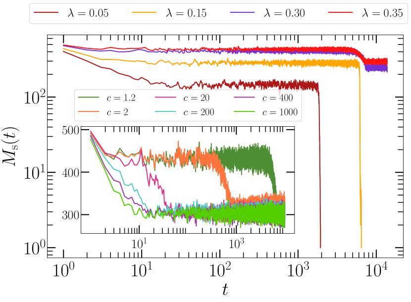
Let us illustrate the overall qualitative phenomenlogy of the model, common for generic values of $M$, $N$ and $c$. A crucial observable is the number of surviving opinions $M_{s}(t)$ as function of time, which plays the role of the order parameter of the system. In the absence of personalized information (that is for $\lambda=0$), for a homogeneous initial condition with $M_{s}(0)=M$ states, the average value of $M_{s}(t)$ satisfies for $t\ll N$ Starnini, Baronchelli, and Pastor-Satorras (2012)

$$M_{s}(t)=\frac{M}{1+\frac{M}{N}t}.$$ (5)

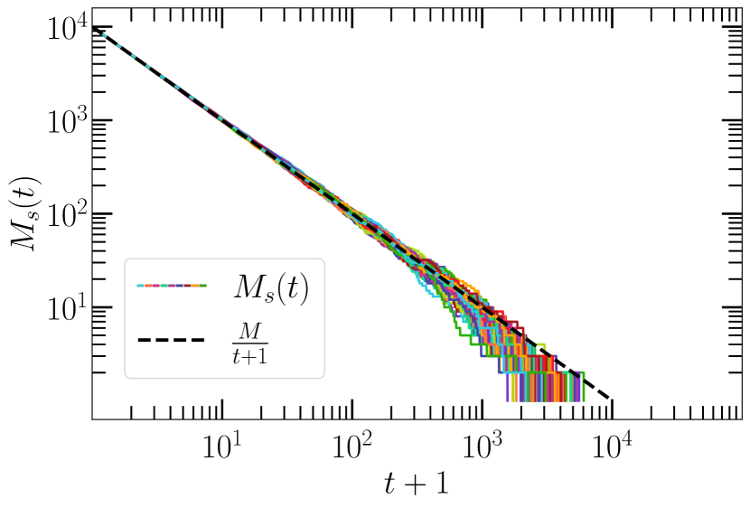
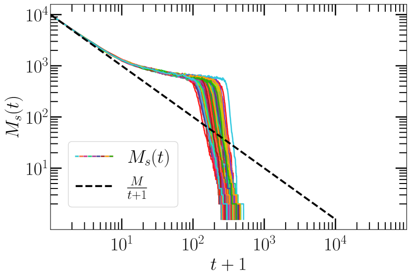
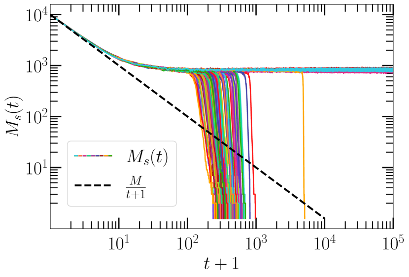
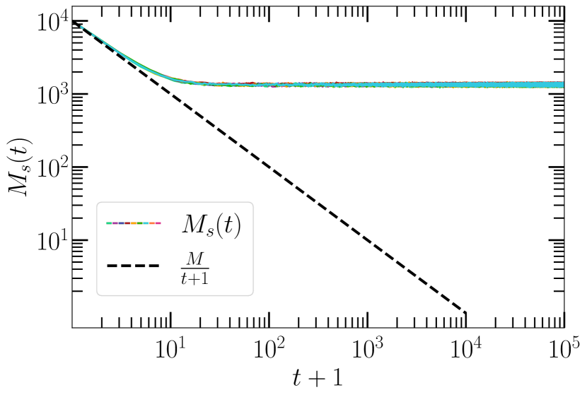
For times of the order of $N$, $M_{s}$ reaches the value $M_{s}=1$, implying an ordered configuration (consensus) in which all agents share the same opinion, as also shown in Fig. 1a. Notice also that there is an intrinsic timescale $t_{0}=N/M$ in Eq. (5) such that $M_{s}$ remains constant and equal to $M_{s}(0)$ for times up to $t_{0}$. As $\lambda$ increases deviations from Eq. (5) start to appear, but the system keeps reaching the ordered state after a sufficiently large amount of time, see Fig. 1b. The behavior changes as $\lambda$ approaches the threshold $\lambda_{c}$; in this case consensus can still be reached, but in some realizations the system remains trapped in a stable disordered state (also denoted as polarized state) characterized by the presence of more than one opinion (Fig. 1c). Finally, for $\lambda$ substantially larger than $\lambda_{c}$, the system never reaches consensus and the asymptotic state is always the disordered one (Fig. 1d). This qualitative phenomenology is observed independently of the value of $c$ (provided that $c>1$). This parameter only determines the possible presence of an initial transient dominated by the randomness of personalized information in the first time steps, as shown Fig. 2. Indeed for $c=1+\delta$ with $\delta\ll 1$ the probability of PI fields, Eq. (3), can be approximated as

$$P\left[n^{(k)}_{i}\right]=\frac{(1+\delta)^{n_{i}^{(k)}}}{\sum_{j=1}^{M}(1+\delta)^{n_{i}^{(j)}}}\approx\frac{1+n_{i}^{(k)}\delta}{M+\delta\sum_{j=1}^{M}n_{i}^{(j)}}.$$

Exploiting the fact that $\sum_{j=1}^{M}n_{i}^{(j)}$ is nothing but the number of times agent $i$ has been updated and that going from $t$ to $t+1$ each agent is on average updated once we have $\sum_{j=1}^{M}n_{i}^{(j)}\approx t$ so that

$$P\left[n^{(k)}_{i}\right]\approx\frac{1+n_{i}^{(k)}\delta}{M+t\delta}\approx\frac{1}{M}+\frac{\delta}{M}\left(n_{i}^{(k)}-\frac{t}{M}\right).$$

Since $0<n_{i}^{(k)}<t$ this implies

$$\frac{1}{M}-\delta\frac{t}{M^{2}}<P\left[n^{(k)}_{i}\right]<\frac{1}{M}+\delta\frac{t}{M}\left(1-\frac{1}{M}\right).$$

As a consequence $P\left[n^{(k)}_{i}\right]=\frac{1}{M}+O(\delta t)$ and so for $\delta$ small the dynamics is initially equal to that of a multistate voter model with external random field. This produces the observed transient. A detailed analysis of the multistate voter model in presence of random external information is beyond the scope of this work, the interested reader can find further details in Herrerías-Azcué and Galla (2019). In order to determine an upper bound of the $c_{th}$ above which no transient is observed, let us consider the first update of agent $i$ and let us suppose that opinion $m$ is selected. As a consequence the probability of the corresponding PI field for the successive update is

$$P\left[e_{i}=k\right]=\begin{dcases}\frac{c}{c+M-1}\ \text{for }k=m\\ \frac{1}{c+M-1}\ \text{for }k\neq m.\end{dcases}$$

If the probability of the PI to be in state $m$ is larger than the probability of being in any other state, a reinforcing loop gets established and the PI gets more and more polarized along opinion $m$. This implies that a sufficient condition for observing a polarized PI already after the first step is

$$P\left[e_{i}(\delta t)=m\right]>\sum_{k\neq m}P\left[e_{i}(\delta t)=k\right],$$

which implies

$$\frac{c}{c+M-1}>\frac{M-1}{c+M-1}$$

yielding a threshold value

$$c_{th}=M-1.$$ (6)

Fig. 2 shows that this estimate is an upper bound of the real $c_{th}$. The duration of the transient governed by a random external field gets shorter as $c$ is increased and it is completely absent for $c\approx c_{th}=999$. Since $c$ plays only a marginal role, in the rest of the paper we focus on the case $c>c_{th}$ so as to remove the initial transient.

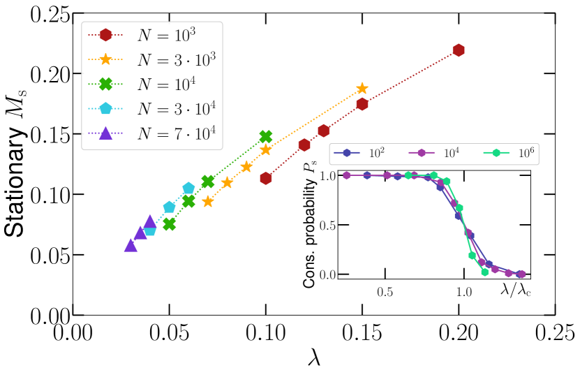
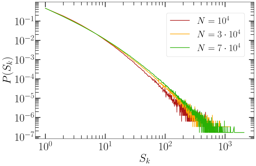
Finally, we illustrate the nature of the transition observed as $\lambda$ is varied. As evident from Fig. 1, around the transition different realizations of the process lead to different outcomes: either consensus or a stationary state. The transition is characterized by the variation, as a function of $\lambda$, of the fraction $P_{s}$ of runs reaching a stationary state (Fig. 3(a),inset). As it is possible to see, the larger is $N$, the sharper the transition becomes. Moreover, since for large $N$ the critical threshold $\lambda_{c}$ goes to zero (see Subsec. III.3 and figures therein) and the transition gets very sharp, this implies that in large systems even an infinitesimal amount of personalized information is sufficient to make the reaching of consensus impossible. The main panel of Fig. 3(a) displays how the fraction of surviving opinions in the stationary state $M_{s}(t\to\infty)/M=M_{s}^{\infty}/M$, averaged only over surviving runs, varies as a function of $\lambda$. The quantity $M_{s}^{\infty}/M$ grows in a continuous fashion, starting from a finite value decreasing with $N$. This suggests that in the large $N$ limit the transition is continuous, as also confirmed by inspecting the distribution of $S_{k}(t\to\infty)=S_{k}^{\infty}$, the number of agents polarized along opinion $k$ in the stationary state. When $c>c_{th}$ the number of polarized agents $S_{k}$ along opinion $k$ is given by the number of agents such that $n_{i}^{(k)}>n_{i}^{(j)}$ for any $j\neq k$, since, in this case, the personalized information suggest the most chosen opinion. Indeed, by looking at Fig. 3(b) it is clear that such a distribution decays as a power-law for $\lambda=\lambda_{c}$, with a nontrivial exponent approximately equal to 2.8 (for $N=M$).

(a)

(b)

Figure 3: a) Main: Stationary value of the fraction $M_{s}$ of opinions, for $M=N$, averaged only over surviving runs. Inset: Probability that consensus is reached as a function of $\lambda$ for $N=10^{2}$, $10^{4}$, $10^{6}$ and $M=20$. As $N$ increases the transition between consensus and polarization becomes sharper and sharper. b) Probability distribution of the number of agents $S_{k}$ polarized along opinion $k$ at criticality for $N=M$. This has been obtained by letting the system evolve toward the stationary state and then performing a binning over the $S_{k}$ so to obtain their histogram. Note that such an histogram corresponds to a single realization of the system.

III Analytical approach

As shown above, the phenomenology of the model is only marginally influenced by the parameter $c$. Therefore consider the case $c\gg c_{th}$ which can be more easily handled analytically. Indeed in such a situation the probability of the PI field $e_{i}$ is strongly peaked on the opinion more frequently held by agent $i$ and Eq. (3) reduces to

$$P\left[e_{i}=k\right]=\delta_{k,m},$$ (7)

where $m$ is the opinion which satisfies

$$m=\underset{k}{\text{argmax}}\left[n_{i}^{(k)}\right].$$

In other words the PI suggests only the favorite opinion in the past. Our goal is to derive, under the assumption of large $c$, analytical estimates of the critical value $\lambda_{c}$ for generic large values of $N$ and $M$.

III.1 Stability of polarized states

(a)

(b)

Figure 4: Temporal evolution of $N_{\max}-N/M$, compared with the critical value $Nm_{c}(\lambda)$ for $N=10^{4}$, $M=200$: a) $\lambda=0.07$; b) $\lambda=0.08$. Different colors correspond to different simulations.

Let us consider an agent $i$ in state $\sigma_{i}$ and let us assume that its PI is polarized along opinion $m$. Combining Eqs. (4) and (7) we can write the transition probability of this agent  as

$$W\left(\sigma_{i}\to k\right)=\begin{dcases}\frac{1}{N}\left[\lambda+(1-\lambda)\frac{N_{k}}{N}\right]&\text{ for }k=m\\ \frac{1}{N}(1-\lambda)\frac{N_{k}}{N}&\text{ for }k\neq m.\end{dcases}$$ (8)

For the overall stability of the polarized state, the PI field $e_{i}$ should remain polarized on opinion $m$ so as to keep the agent we are considering fixed (on average) on this same opinion. This requires the transition probability to opinion $m$ to be larger than the transition probability to any other opinion $l$, otherwise $n_{i}^{(l)}$ would grow faster than $n_{i}^{(m)}$ and the PI would eventually depolarize and then polarize along opinion $l$. As a consequence, in order for the polarized state to be stable it must be

$$W\left(\sigma_{i}\to m\right)>W\left(\sigma_{i}\to l\right)\leavevmode\nobreak\ \leavevmode\nobreak\ \leavevmode\nobreak\ \leavevmode\nobreak\ \leavevmode\nobreak\ \leavevmode\nobreak\ \forall l\neq m,$$

which yields, using Eq. (8)

$$\frac{N_{m}-N_{l}}{N}>-\frac{\lambda}{1-\lambda}=-m_{c}(\lambda).$$ (9)

Here, in analogy with De Marzo, Zaccaria, and Castellano (2020), we defined the critical magnetization $m_{c}(\lambda)$ as

$$m_{c}(\lambda)=\frac{\lambda}{1-\lambda}.$$ (10)

We can then repeat this same reasoning but considering an agent $j$ whose PI field $e_{j}$ is polarized along opinion $l$. This leads to

$$\frac{N_{m}-N_{l}}{N}<m_{c}(\lambda).$$

Combining this expression with Eq. (9) we obtain the following necessary condition for a polarized state to be stable

$$\left|\frac{N_{m}-N_{l}}{N}\right|<m_{c}(\lambda)\leavevmode\nobreak\ \leavevmode\nobreak\ \leavevmode\nobreak\ \leavevmode\nobreak\ \forall(l,m).$$ (11)

By introducing the partial magnetization $m_{k}$ along opinion $k$, we can also rewrite this constraint as

$$m_{k}=\frac{N_{k}-\sum_{l\neq k}N_{k}}{N}=\frac{2N_{k}-N}{N}.$$

In this way Eq. (11) becomes

$$\left|\frac{m_{m}-m_{l}}{2}\right|<m_{c}.$$ (12)

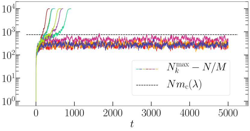
The conclusion if the difference between any two magnetizations is smaller than the threshold $m_{c}$ then the polarized state is stable. Note, however, that this condition is very strict and a polarized state can be stable on average even if there are some opinions held by a small number of agents not fulfilling it. Indeed in such a situation these opinions will be absorbed by the others, but still consensus will not be reached. As a consequence what really matters is that (11) is fulfilled when considering the most common opinion whose size is $N_{max}$ and the average opinion size given by $N/M$. The condition ensuring the system not to reach consensus is thus

$$N_{max}-\frac{N}{M}<Nm_{c}(\lambda).$$ (13)

Fig. 4 checks and confirms the validity of this argument in numerical simulations. Note that $m_{c}$ is larger than 1 for $\lambda>1/2$ and so, as in the voter model with personalized information, above $\lambda=1/2$ an opinion can survive even with only a single agent supporting it.

III.2 Polarization time

Figure 5: Temporal evolution of the $Q(n_{i}^{(k)})$ distribution as a function of time. Data are for $c=400,$ $N=10^{6}$, $M=20$, $\lambda=0.07$. The component with high mean value represents agents polarized along opinion $k$; the component with low mean value represents agents unpolarized or polarized along other opinions.

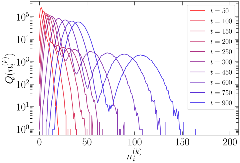
In deriving Eq. (12) we assumed all PI fields to be polarized on a certain opinion, meaning that for any $i$ there is only one $k$ such that $n_{i}^{(k)}$ is maximum. However initially $n_{i}^{(k)}=0$ for all pairs $(i,k)$ and the randomness of voter updates implies the occurrence of several ties between the various $n_{i}^{(k)}$. The assumption that PI fields are polarized starts to be valid only after a polarization time $t^{*}>0$. In order to compute this time we write down the master equation for the distribution of the $n_{i}^{(k)}$ values, $Q(n_{i}^{(k)})$, that reads

$$\frac{dQ\left(n_{i}^{(k)}\right)}{dt}=NR\left(n_{i}^{(k)}-1\right)Q\left(n_{i}^{(k)}-1\right)-NR\left(n_{i}^{(k)}\right)Q\left(n_{i}^{(k)}\right),$$ (14)

where we introduced the single transition probability

$$NR\left(n_{i}^{(k)}\right) =\left(1-\lambda\right)\frac{N_{k}}{N}+\lambda P\left(e_{i}=k\right)$$

$$\approx\left(1-\lambda\right)\frac{1}{M_{s}(t)}+\lambda P\left(e_{i}=k\right).$$ (15)

Here we assumed that all surviving opinions share approximately the same number of agents and so we can make the approximation ${N_{k}}/{N}\approx{1}/{M_{s}(t)}$. Now, considering opinion $k$, only a fraction $S_{k}/N$ of the agents is polarized along this opinion and thus we assume that the distribution $Q(n_{i}^{(k)})$ is formed by two normalized components $Q_{1}$ and $Q_{2}$ corresponding to the two types of agents: those polarized on opinion $k$ (component $Q_{2}$) and those polarized on any other opinion or not polarized at all (component $Q_{1}$). We can then write $Q$ as a bimodal distribution

$$Q\left(n_{i}^{(k)}\right)=\left(1-\frac{S_{k}}{N}\right)Q_{1}\left(n_{i}^{(k)}\right)+\frac{S_{k}}{N}Q_{2}\left(n_{i}^{(k)}\right).$$

Both components evolve according to the same general master equation Eq. (14), but the transition rates are different. For what concerns the polarized component $Q_{2}$ we have

$$NR\left(n_{i}^{(k)}\right)=\left(1-\lambda\right)\frac{1}{M_{s}(t)}+\lambda$$

and using this expression and Eq. (14) we can compute both the mean value $n_{2}$ and the variance $\sigma_{2}^{2}$ of the distribution $Q_{2}$ for polarized agents, finding

$$n_{2}=\sigma_{2}^{2}=\int_{0}^{t}dt^{\prime}\left(\frac{1-\lambda}{M_{s}(t^{\prime})}+\lambda\right),$$ (16)

Analogously, the transition rate of the component $Q_{1}$, corresponding to agents not polarized on opinion $k$, is

$$NR\left(n_{i}^{(k)}\right)=\left(1-\lambda\right)\frac{1}{M_{s}(t)}$$

and so the mean value $n_{1}$ and the variance $\sigma_{1}^{2}$ are

$$n_{1}=\sigma_{1}^{2}=\int_{0}^{t}dt^{\prime}\left(\frac{1-\lambda}{M_{s}(t^{\prime})}\right).$$ (17)

Detailed computations are reported in Appendix A.

Looking at Eqs. (16) and (17) it is clear that initially the two components are indistinguishable since they both have null mean and variance. However, having different velocities they tend to separate over time. This behavior is shown in Fig. 5. Until $Q_{1}$ and $Q_{2}$ are superposed there is no real distinction between polarized and unpolarized agents, as all agents can change their preferred opinion in one or few voter updates. Consequently we identify the polarization time $t^{*}$ introduced above as the time when the two components split for the first time. This can be readily determined by imposing the distance between the two peaks to be equal to their widths, that is

$$n_{2}(t^{*})-n_{1}(t^{*})=2\left[\sqrt{\sigma_{1}^{2}(t^{*})}+\sqrt{\sigma_{2}^{2}(t^{*})}\right],$$

where the factor $2$ is somewhat arbitrary and does not influence the scaling of $t^{*}$. Substituting Eqs. (16) and (17) into this last expression we come up with an implicit integral expression for the polarization time $t^{*}$

$$t^{*}=\frac{2}{\lambda}\left\{\sqrt{\int_{0}^{t^{*}}\left[\frac{1-\lambda}{M_{s}(t)}+\lambda\right]dt^{\prime}}+\sqrt{\int_{0}^{t^{*}}\frac{1-\lambda}{M_{s}(t)}dt^{\prime}}\right\}$$ (18)

III.3 The transition point

Once the polarization time has been obtained we can turn to the determination of the critical parameter $\lambda_{c}$. The idea is the following: In the initial stage of the dynamics, the numbers of agents holding the different opinions, $N_{l}$, tend to fluctuate and their differences tend to grow over time. If this growth is slow enough, at the polarization time $t^{*}$ the condition for the stability of polarized states, Eq. (13) is satisfied. In such a case the disordered state with multiple coexisting opinions is stable and persists forever. Conversely, if at $t^{*}$ Eq. (13) is violated, the system will eventually evolve toward the consensus state. The condition for $\lambda_{c}$ thus reads

$$x_{\max}(t^{*})=N_{\max}(t^{*})-\frac{N}{M}=N\frac{\lambda_{c}}{1-\lambda_{c}}.$$ (19)

By means of numerical simulations and a simple scaling argument (see Appendix 8) we determine that for $M\ll N$ $x_{\max}(t)$ scales as

$$x_{\max}(t)\sim\gamma\frac{N^{1/2}}{M}t^{3/2},$$ (20)

where $\gamma\approx 1/4$ is a numerical constant. We also derived an equation for the time growth of $N_{k}-N/M$ and we checked that the temporal scaling of $x_{\max}(t)$ is consistent with this expression, see Appendix C. Replacing this last expression into Eq. (19) we obtain an equation for $\lambda_{c}$

$$\gamma\frac{N^{1/2}}{M}{t^{*}}^{3/2}=N\frac{\lambda_{c}}{1-\lambda_{c}},$$

implying

$$\lambda_{c}=\frac{\gamma\frac{N^{1/2}}{M}\left[t^{*}(\lambda_{c})\right]^{3/2}}{N+\gamma\frac{N^{1/2}}{M}\left[t^{*}(\lambda_{c})\right]^{3/2}}.$$ (21)

Eq. (21), together with Eq. (18) for the polarization time, provide a closed system of equations in $\lambda_{c}$ and $t^{*}$

$$\begin{dcases}t^{*}=\frac{2}{\lambda_{c}}\left\{\sqrt{\int_{0}^{t^{*}}\left[\frac{1-\lambda_{c}}{M_{s}(t^{\prime})}+\lambda_{c}\right]dt^{\prime}}+\sqrt{\int_{0}^{t^{*}}\frac{1-\lambda_{c}}{M_{s}(t^{\prime})}dt^{\prime}}\right\}\\ \lambda_{c}=\frac{\gamma\frac{N^{1/2}}{M}(t^{*})^{3/2}}{N+\gamma\frac{N^{1/2}}{M}(t^{*})^{3/2}}.\end{dcases}$$ (22)

In order to solve this system we need an explicit expression for the number $M_{s}(t)$ of surviving opinions. We consider two possible assumptions, which are expected to be fairly accurate for different values of $M$ and $N$. Here we limit ourselves to report the main results, the interested reader can find detailed calculations in Appendix D.

III.4 $\mathbf{M\ll N}$

If the number of opinions in much smaller than the number of agents, each opinion is initially shared by a large number of individuals. As a consequence during a first time interval no opinion disappears and it is reasonable to make the approximation

$$M_{s}(t)=M$$

In this way Eq. (22) can be rewritten as

$$\begin{dcases}t^{*}=\frac{4}{\lambda_{c}^{2}}\left[\sqrt{\frac{1-\lambda_{c}}{M}+\lambda_{c}}+\sqrt{\frac{1-\lambda_{c}}{M}}\right]^{2}\\ \lambda_{c}=\frac{\gamma\frac{N^{1/2}}{M}(t^{*})^{3/2}}{N+\gamma\frac{N^{1/2}}{M}(t^{*})^{3/2}}.\end{dcases}$$ (23)

Depending on how large $M$ is with respect to $N$, the solutions of this system scale in different ways.

• $\mathbf{M\ll N^{1/3}}$
  

  $$\begin{cases}t^{*}\approx 4(MN)^{1/4}\\ \lambda_{c}\approx 2\left(M^{5}N\right)^{-1/8}.\end{cases}$$ (24)

• $\mathbf{N^{1/3}\ll M\ll N}$
  

  $$\begin{cases}t^{*}\approx 2^{8/5}\left(NM^{2}\right)^{1/5}\\ \lambda_{c}\approx 2^{2/5}\left(NM^{2}\right)^{-1/5}.\end{cases}$$ (25)

III.5 $\mathbf{M=N}$

If $M=N$ each agent has initially a different opinion. Hence, even during the first time steps, some opinions disappear by chance. In this case we can approximate the surviving opinions $M_{s}(t)$ with the expression valid for the simple multistate voter model, Eq. (5), that is for $M=N$,

$$M_{s}(t)=\frac{N}{1+t}.$$ (26)

Substituting this expression in Eq. (22) and imposing $M=N\gg 1$, $\lambda_{c}\ll 1$ we obtain the following system

$$\begin{dcases}t^{*}=\frac{32N^{1/2}+8\lambda_{c}N}{2\left(\lambda_{c}^{2}N-16\right)}\\ \lambda_{c}=\frac{\gamma N^{-1/2}\left[t^{*}(\lambda_{c})\right]^{3/2}}{N+\gamma N^{-1/2}\left[t^{*}(\lambda_{c})\right]^{3/2}},\end{dcases}$$ (27)

whose solution scales as

$$\begin{cases}t^{*}\approx 2^{4/3}N^{2/3}\\ \lambda_{c}\approx 4N^{-1/2}\end{cases}$$ (28)

(a) $M=20\ll N$.

(b) $M=200\ll N$.

(c) $M=N$.

Figure 6: Comparison of analytical predictions for the threshold $\lambda_{c}$ and numerical estimates of it

IV Numerical simulations

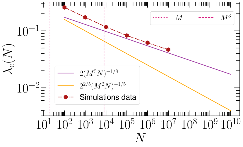
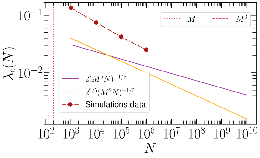
We now compare theoretical predictions with numerical simulations. We iterate MVM dynamics for various values of $M$ and $N$ up to $t=2000$ and we determine the fraction of times $P_{s}(\lambda)$ the system has reached consensus. We take as numerical estimate of $\lambda_{c}$ the values such that $P_{s}(\lambda_{c})=1/2$.

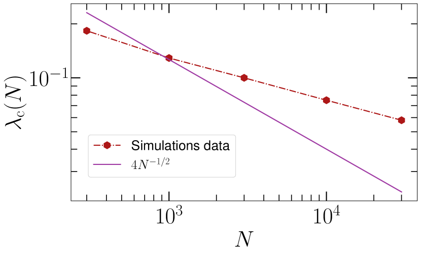
For fixed value of $M$ and increasing size $N$, the analytical results predict initially a scaling regime given by Eq. (25) as long as $N$ is much larger than $M$ but much smaller than $M^{3}$, followed by a scaling given by Eq. (24). For $M=20$, the first regime spans a short interval of $N$ values. In Fig. 6(a) we see only a hint of the associated scaling, while for larger values of $N$ the agreement between theory and numerics is very good. For $M=200$ instead (see Fig. 6(b)), the first regime extends to much larger values of $N$, so that feasible values of $N$ lie only in this regime. In this case $\lambda_{c}$ nicely scales as $N^{-1/5}$, as predicted by Eq. (25), although the prefactor is not predicted exactly.

For the case $M=N$ instead, Figure 6(c) show that the theory is not able to catch the correct scaling. This mismatch has various potential origins. Indeed using Eq. (26) for the temporal dependence of $M_{s}(t)$ is a quite rough approximation, as the number of different opinions actually decays much more slowly over time. But also the use of Eq. (19) for $x_{\max}(t)$ is not warranted for $M=N$. A deeper understanding of the phenomenology of the case $M=N$ remains an interesting open question.

V Conclusions

In this paper we have introduced and analyzed a multistate voter model where the coupling with an external history-dependent individual field mimics the effect of personalized recommendation algorithms in online social media. A population of agents, initially having different opinions, reaches consensus on a single opinion or remains polarized on multiple different opinions, depending on the strength of personalized information. The phenomenology is governed by the competition between the fluctuations induced by voter dynamics and the tendency, due to personalized information, to bind agents to the opinion they adopted most frequently in the past. By means of arguments based on this physical picture, we estimated analytically the critical threshold between the two regimes, obtaining a reasonable agreement with simulations for $M\ll N$. Conversely, the dynamics when the initial number of opinions is comparable with the number of agents seems to elude our approach.

From a more general point of view, our study indicates how difficult reaching consensus is, in the presence of personalized recommendations. For any number $M$ of initial opinions the threshold $\lambda_{c}$ tends to vanish when the number of agents $N$ diverge. This means that no matter how weak is the coupling with the personalized information, if the system is large enough polarization unavoidably arises. In this respect, note that voter dynamics is extremely favorable to the establishment of consensus: for any interaction pattern, consensus is necessarily reached for any finite number of interacting individuals. The addition of a personalized recommendation completely changes this picture, at least for large systems. For a finite number of interacting agents instead consensus is still reached if the strength of personalized information is small enough. The transition between the two regimes exhibits nontrivial features that may be the focus of future activity along with generalizations to include nontrivial interaction patterns or a different functional dependence between the probability distribution of the personalized information and the number of times an opinion has been selected in the past.

A natural extension of this work would be to analyze more realistic recommendation algorithms. With respect to this, a promising possibility is to consider collaborative filtering algorithms Schafer et al. (2007), which are based on similarities among the history of different users or opinions instead of considering only the history of the user itself. This typology of algorithm is used in real life applications Linden, Smith, and York (2003); Smith and Linden (2017), but still it is sufficiently simple to try an analytical study of its effects on opinion dynamics models.

Appendix A Moments of the distribution of $n_{i}^{(k)}$

(a)

(b)

(c)

Figure 7: (a) Temporal evolution of $x_{\max}(t)$, $y_{\max}(t)$ and their difference for $N=10^{7}$, $M=20$, $\lambda\approx\lambda_{c}$. (b) Collapse plot to check the scaling (20) with respect to $N$; $M=20$ and $\lambda\approx\lambda_{c}$. (c) Collapse plot to check the scaling (20) with respect to $M$; $N=10^{7}$ and $\lambda\approx\lambda_{c}$.

Let us consider the distribution $Q\left(n_{i}^{(k)},t\right)$, where $n_{i}^{(k)}$ is defined as the number of times agent $i$ has chosen or confirmed opinion $k$ in the past. The evolution of this distribution is given by

$$Q\left(n_{i}^{(k)},t+\delta t\right) =R\left(n_{i}^{(k)}-1\right)Q\left(n_{i}^{(k)}-1,t\right)+$$

$$+\left[1-R\left(n_{i}^{(k)}\right)\right]Q\left(n_{i}^{(k)},t\right).$$

Expanding the left hand side for small $\delta t=1/N$ we obtain which yields Eq. (14)

$$\frac{dQ\left(n_{i}^{(k)}\right)}{dt} =NR\left(n_{i}^{(k)}-1\right)Q\left(n_{i}^{(k)}-1\right)-$$

$$-NR\left(n_{i}^{(k)}\right)Q\left(n_{i}^{(k)}\right).$$ (29)

Now we consider the two components $Q_{1}\left(n_{i}^{(k)},t\right)$ and $Q_{2}\left(n_{i}^{(k)},t\right)$ introduced in III.2 and we compute their mean value and variance. We recall that $Q_{2}$ corresponds to agents whose PI are polarized along $k$, while $Q_{1}$ to the remaining agents, and that both components evolve according to the same master equation Eq. (14), but with different transition rates. The general equation for the drift of the distribution (also called average drift in the following) is

$$\nu=\frac{d\left\langle n_{i}^{(k)}\right\rangle}{dt}=\sum_{n_{i}^{k}}n_{i}^{(k)}\frac{dQ\left(n_{i}^{(k)}\right)}{dt}$$

and using Eq. (29) we obtain

$$\nu=\sum_{n_{i}^{k}} n_{i}^{(k)}\left[NR\left(n_{i}^{(k)}-1\right)Q\left(n_{i}^{(k)}-1\right)\right.-$$

$$-\left.NR\left(n_{i}^{(k)}\right)Q\left(n_{i}^{(k)}\right)\right]=$$

$$= \sum_{n_{i}^{k}}NR\left(n_{i}^{(k)}\right)Q\left(n_{i}^{(k)}\right)$$ (30)

Analogously the evolution of the second moment is

$$\frac{d\left\langle\left(n_{i}^{(k)}\right)^{2}\right\rangle}{dt}=\sum_{n_{i}^{k}}\left(n_{i}^{(k)}\right)^{2}\frac{dQ\left(n_{i}^{(k)}\right)}{dt},$$

that using Eq. (29) becomes

$$\frac{d\left\langle\left(n_{i}^{(k)}\right)^{2}\right\rangle}{dt}=\sum_{n_{i}^{k}} \left(n_{i}^{(k)}\right)^{2}\left[NR\left(n_{i}^{(k)}-1\right)Q\left(n_{i}^{(k)}-1\right)\right.-$$

$$-\left.NR\left(n_{i}^{(k)}\right)Q\left(n_{i}^{(k)}\right)\right]=$$

$$=\sum_{n_{i}^{k}} \left(n_{i}^{(k)}+1\right)^{2}NR\left(n_{i}^{(k)}\right)Q\left(n_{i}^{(k)}\right)-$$

$$-\left(n_{i}^{(k)}\right)^{2}NR\left(n_{i}^{(k)}\right)Q\left(n_{i}^{(k)}\right)=$$

$$= \nu+2\sum_{n_{i}^{k}}n_{i}^{(k)}NR\left(n_{i}^{(k)}\right)Q\left(n_{i}^{(k)}\right),$$ (31)

where we used Eq. (30). Let us firstly consider agents polarized along $k$ and so $Q_{2}$, the transition rate is

$$NR_{2}\left(n_{i}^{(k)}\right)=(1-\lambda)\frac{1}{M_{s}(t)}+\lambda.$$

and putting this expression into Eqs. (30) and (31) we get

$$\begin{dcases}\nu_{2}=(1-\lambda)\frac{1}{M_{s}(t)}+\lambda\\ \frac{d\left\langle\left(n_{i}^{(k)}\right)^{2}\right\rangle_{2}}{dt}=\left[(1-\lambda)\frac{1}{M_{s}(t)}+\lambda\right]\left(1+2n_{2}\right),\end{dcases}$$ (32)

where we defined $n_{2}=\left\langle n_{i}^{(k)}\right\rangle_{2}$. Analogously for the component $Q_{1}$ it holds

$$NR_{1}\left(n_{i}^{(k)}\right)=(1-\lambda)\frac{1}{M_{s}(t)}$$

and so

$$\begin{dcases}\nu_{1}=(1-\lambda)\frac{1}{M_{s}(t)}\\ \frac{d\left\langle\left(n_{i}^{(k)}\right)^{2}\right\rangle_{1}}{dt}=(1-\lambda)\frac{1}{M_{s}(t)}\left(1+2n_{2}\right).\end{dcases}$$ (33)

Finally, considering that

$$n=\int_{0}^{t}\nu\cdot dt^{\prime}$$

$$\sigma_{n}^{2}=\left\langle\left(n_{i}^{(k)}\right)^{2}\right\rangle-\langle n_{i}^{(k)}\rangle^{2}$$

$$\frac{d\sigma^{2}}{dt}=\frac{d\left\langle\left(n_{i}^{(k)}\right)^{2}\right\rangle}{dt}-2\left\langle n_{i}^{(k)}\right\rangle\frac{d\left\langle n_{i}^{(k)}\right\rangle}{dt}$$

we can write the expressions for the mean value and variance of both components

$$\begin{dcases}n_{2}(t)=\sigma_{2}^{2}(t)=\int_{0}^{t}dt^{\prime}\left(\frac{1-\lambda}{M_{s}(t^{\prime})}+\lambda\right)\\ n_{1}(t)=\sigma_{1}^{2}(t)=\int_{0}^{t}dt^{\prime}\frac{1-\lambda}{M_{s}(t^{\prime})}.\\ \end{dcases}$$ (34)

These are Eqs. (16) and (17).

Appendix B Scaling of $x_{\max}(t)$

Figure 8: Growth of the maximum of a multinomial distribution with $M$ equally probable classes as a function of the number of extractions $t$ for different values of $M$. We denote by $n_{k}$ the number of counts in the $k$th classe. We plotted the quantity $\left\{\max\left[n_{k}\right]-\langle n_{k}\rangle\right\}M^{1/4}$ to highlight the scaling with respect to $M$ and we averaged over $25$ different realizations of the process.

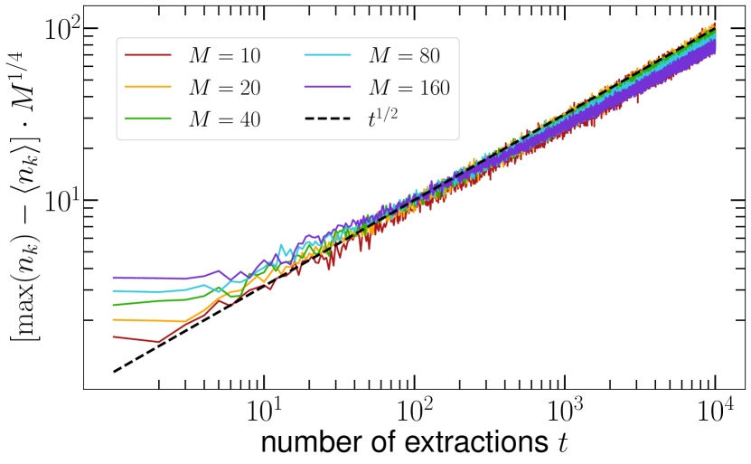
As discussed in the main text, near the transition point the quantity $x_{\max}(t)=N_{\max}(t)-N/M$ satisfies Eq. (20), that is

$$x_{\max}(t)=\gamma\frac{N^{1/2}}{M}t^{3/2}.$$

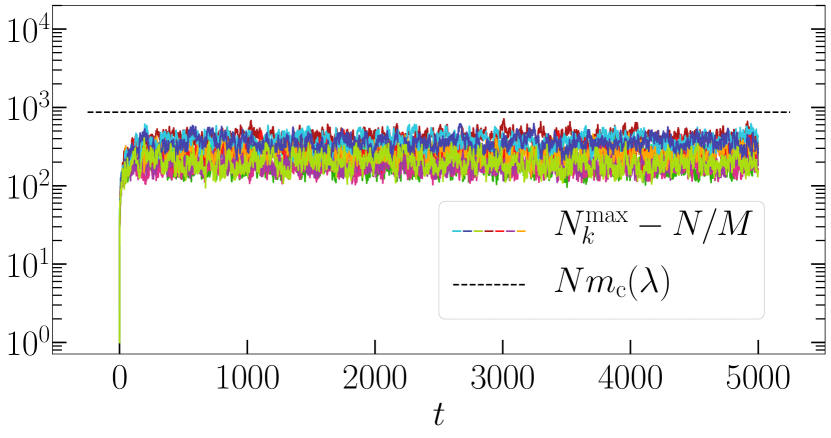
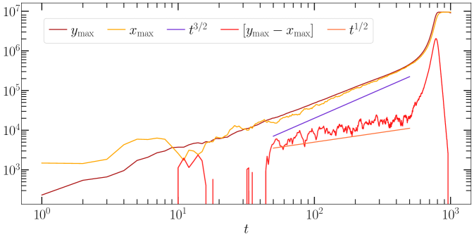
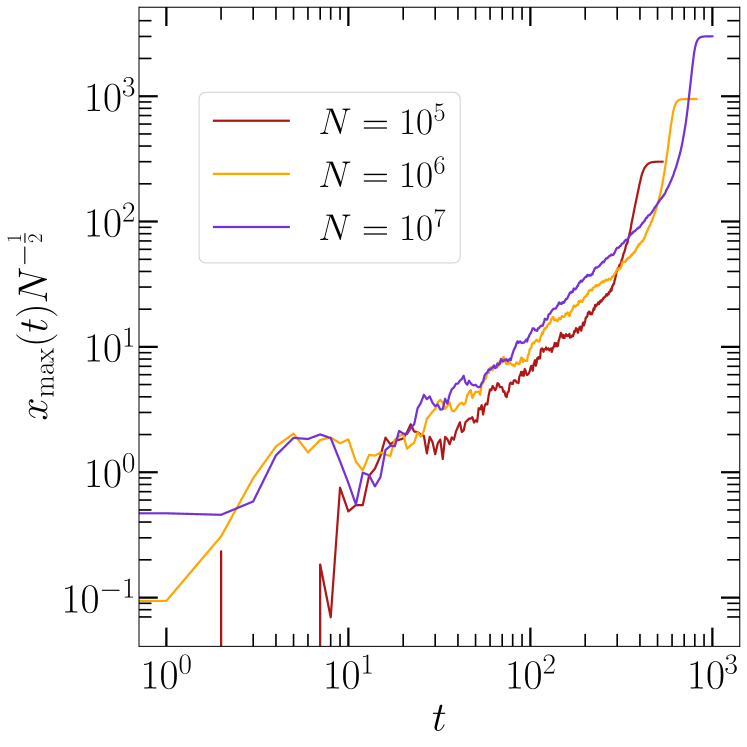
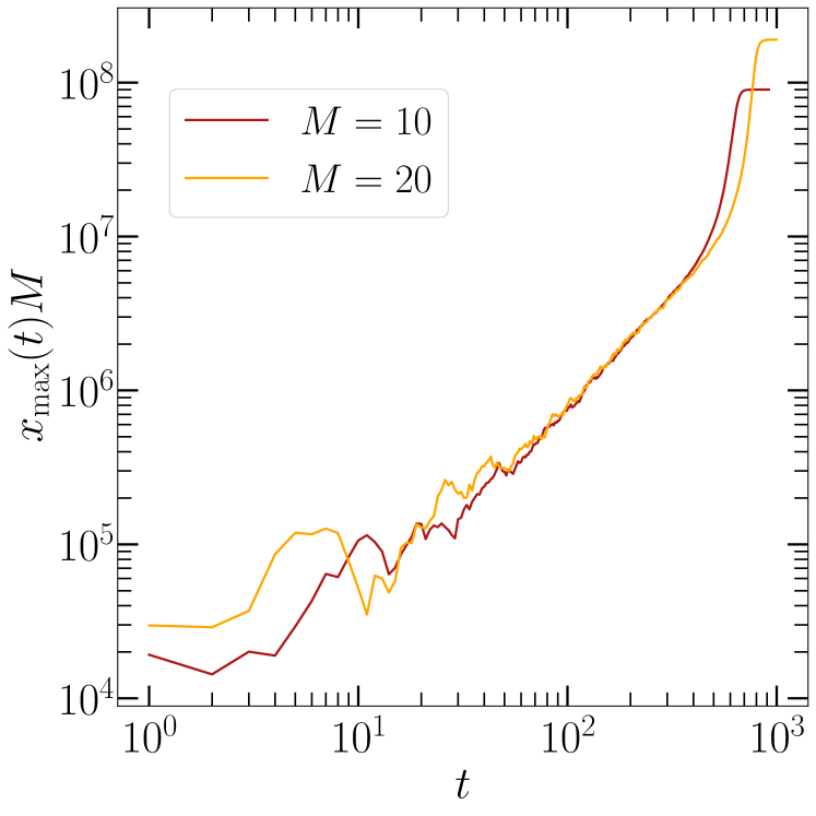
This is shown in Fig. 7, where we test both the evolution in time and the scaling with respect to $M$ and $N$. The latter can be also explained by considering the dynamics during the first steps. Initially all $n_{i}^{(k)}$ are null and all opinions are equally common, so each agent, when updated, chooses an opinion with uniform probability. This regime lasts up to $t<\bar{t}$, where $\bar{t}$ is defined as the time when the $n_{i}^{(k)}$ becomes statistically different from zero and so the PI stops to be completely random. This implies that for fixed $i$ and up to $\bar{t}$ the $M$ variables $n_{i}^{(k)}$ are distributed according to a multinomial distribution with uniform probability $1/M$. The multinomial regime ends when the maximum $\max_{k}\left[n_{i}^{(k)}\right]$ exceeds the average $\langle n_{i}^{(k)}\rangle_{k}$ by one, since when this occurs the external information stops to suggest random opinions. The mean value after $t$ extractions satisfies $\langle n_{i}^{(k)}\rangle_{k}=t/M$, while by drawing from a multinomial we numerically determined that $\max_{k}\left[n_{i}^{(k)}\right]-\langle n_{i}^{(k)}\rangle_{k}\approx t^{1/2}M^{-1/4}$, see Fig. 8. We can then obtain the time $\bar{t}$ as

$$\bar{t}^{1/2}M^{-1/4}=1\ \to\ \bar{t}=M^{1/2}.$$ (35)

Now we consider the evolution of the number of agents $N_{k}$ in opinion $k$ in the simple multistate voter model. The transition rates are

$$\begin{dcases}W\left(N_{k}\to N_{k}\pm 1\right)=\frac{1}{\delta t}\frac{N-N_{k}}{N}\frac{N_{k}}{N}\\ W\left(N_{k}\pm 1\to N_{k}\right)=\frac{1}{\delta t}\frac{N-\left(N_{k}\pm 1\right)}{N}\frac{N_{k}\pm 1}{N},\end{dcases}$$ (36)

where $\delta t=1/N$. The master equation for $N_{k}$ is thus

$$P(N_{k},t+ \delta t)=P(N_{k}+1,t)W\left(N_{k}+1\to N_{k}\right)+$$

$$+P(N_{k}-1,t)W\left(N_{k}-1\to N_{k}\right)+$$

$$+\left[1-W\left(N_{k}\to N_{k}-1\right)-W\left(N_{k}\to N_{k}+1\right)\right]P\left(N_{k},t\right).$$

Expanding for $\delta t$ small we get

$$\frac{\partial P(N_{k},t)}{\partial t} \cdot\delta t=W(N_{k}+1\to N_{k})P(N_{k}+1,t)$$

$$+ W(N_{k}-1\to N_{k})P(N_{k}-1,t)+$$

$$- [W(N_{k}+1\to N_{k})+W(N_{k}-1\to N_{k})]P(N_{k},t).$$ (37)

Starting from this master equation we can compute the average drift and the variance of $N_{k}$. The average drift satisfies

$$\nu_{k}= \frac{d\langle N_{k}\rangle}{dt}=\sum_{N_{k}}N_{k}\frac{\partial P(N_{k},t)}{\partial t}$$

$$= \frac{1}{\delta t}\sum_{N_{k}}[W(N_{k}\to N_{k}+1)-W(N_{k}\to N_{k}-1)]P(N_{k},t)=$$

$$= \sum_{N_{k}}\frac{dN_{k}}{dt}P(N_{k},t)=\sum_{N_{k}}\nu_{k}(N_{k})P(N_{k},t),$$ (38)

where we also introduced the drift $\nu_{k}(N_{k})=[W(N_{k}\to N_{k}+1)-W(N_{k}\to N_{k}-1)]/\delta t$. Note that while the average drift $\nu_{k}$ determines how the mean value of the distribution $P(N_{k})$ moves in time, the drift $\nu_{k}(N_{k})$ allows to compute (neglecting diffusion) how a specific value of $N_{k}$ evolves. Using Eqs. (36) we get

$$\nu_{k}=0\ \to\ \left\langle N_{k}(t)\right\rangle=N_{k}(0)=\frac{N}{M}.$$ (39)

Analogously the evolution of the variance is

$$\frac{d\sigma_{k}^{2}}{dt}=\frac{d\left\langle N_{k}^{2}\right\rangle}{dt}-2\left\langle N_{k}\right\rangle\frac{d\left\langle N_{k}\right\rangle}{dt}=\frac{d\left\langle N_{k}^{2}\right\rangle}{dt},$$

where the last equality follows from Eq. (39). Exploiting Eq. (37) we then obtain

$$\frac{d\left\langle N_{k}^{2}\right\rangle}{dt}=\sum_{N_{k}}N_{k}^{2}\frac{\partial P(N_{k},t)}{\partial t}=2\left(\left\langle N_{k}\right\rangle-\frac{1}{N}\left\langle N_{k}^{2}\right\rangle\right),$$

whose solution is

$$\left\langle N_{k}^{2}\right\rangle(t)=\left(\frac{N^{2}}{M^{2}}-\frac{N^{2}}{M}\right)\mathrm{e}^{-2\frac{t}{N}}+\frac{N^{2}}{M}.$$

The variance is thus

$$\sigma_{k}^{2}(t)=\left\langle N_{k}^{2}\right\rangle(t)-\left\langle N_{k}\right\rangle^{2}(t)=\left(\frac{N^{2}}{M}-\frac{N^{2}}{M^{2}}\right)\left(1-\mathrm{e}^{-2\frac{t}{N}}\right).$$ (40)

As also shown in Fig. 1, for small times and small values of $\lambda$ our model with personalized information behaves as the usual voter model. This is due to the fact that for $t<\bar{t}$ the external information is completely random and so, being all opinions equally numerous at the beginning, a voter model-like update or a personalized information update are equivalent. This implies that we can use Eqs. (39) and (40) to determine how $N_{\max}$ and thus $x_{\max}$ evolve for small times even in the presence of personalized information

$$N_{\max}(t)\approx\left\langle N_{k}(t)\right\rangle+\sigma_{k}(t)\ \to\ x_{\max}(t)\approx\sigma_{k}(t).$$

By expanding Eq. (40) for small times we thus obtain

$$x_{\max}(t)\approx\sqrt{2\frac{t}{N}\left(\frac{N^{2}}{M}-\frac{N^{2}}{M^{2}}\right)}\approx 2\sqrt{\frac{N}{M}t}\ \text{ for }t\leq\bar{t},$$

where again we assumed $M\gg 1$. Finally, we know from empirical evidence that for large times it holds $x_{\max}(t)\sim t^{3/2}$; this implies that the functional form of $x_{\max}(t)$ must be

$$x_{\max}(t)=\alpha t^{3/2}+2\sqrt{\frac{N}{M}}t^{1/2}.$$

The prefactor $\alpha$ can now be determined imposing the $t^{3/2}$ scaling to become dominant when the binomial scaling $t^{1/2}$ ends, so for $t=\bar{t}=\sqrt{M}$. This gives

$$\alpha\bar{t}^{3/2}=2\sqrt{\frac{N}{M}}\bar{t}^{1/2}$$

and so

$$\alpha=\frac{N^{1/2}}{M}.$$

This shows that for sufficiently large $t$ it holds

$$x_{\max}(t)\sim\frac{N^{1/2}}{M}t^{3/2}.$$

Appendix C Evolution of $N_{k}-N/M$

The transition rate for $N_{k}$ in the presence of personalized information is

$$W(N_{k}\to N_{k}+1)=(1-\lambda)\frac{N-N_{k}}{N}\frac{N_{k}}{N}+\lambda P_{PI,\to k},$$

where the first term is the usual voter contribution, while the second one is due to PI. Denoting as $S_{k}=Ns_{k}$ the number of agents whose PI is polarized along opinion $k$, we can write the latter as

$$P_{PI\to k}=\frac{N-N_{k}-\sum_{j\neq k}S_{k}}{N}\frac{1}{M_{s}(t)}.$$

Let us explain this expression. Among all the $N$ agents, those already with opinion $k$ do not contribute to the transition rate to opinion $k$, while those whose PI is polarized along $j\neq k$ can make a transition toward $k$ only by a voter update. As a consequence only $N-N_{k}-\sum_{j\neq k}S_{k}$ should be considered in computing the transition probability. Moreover the PI of such agents will be unpolarized and so we can assume that it suggests a random opinion, giving the factor $1/M_{s}(t)$. Analogously

$$W(N_{k}\to N_{k}-1)=(1-\lambda)\frac{N-N_{k}}{N}\frac{N_{k}}{N}+\lambda P_{PI,k\to}$$

with

$$P_{PI,k\to}=\frac{N_{k}-S_{k}}{N}\frac{M_{s}(t)-1}{M_{s}(t)}.$$

Inserting these transition rates in Eq. (38) we can write the drift of $N_{k}$ as

$$\nu_{k}(N_{k})=\frac{\lambda}{M_{s}}\left[N-S-M_{s}\left(N_{k}-S_{k}\right)\right],$$

where we introduced the total number of polarized agents as $S=\sum_{k}S_{k}$. The time evolution of $N_{k}$, neglecting diffusive fluctuations, is thus

$$\frac{dN_{k}}{dt}=\nu_{k}(N_{k})=\lambda\left[\left(S_{k}-\frac{S}{M_{s}}\right)-\left(N_{k}-\frac{N}{M_{s}}\right)\right].$$

For $N\gg M$ and short times we can make the approximation $M_{s}\approx M$ and so defining $y_{k}=S_{k}-S/M$ we arrive at an expression for the time evolution of $x_{k}=N_{k}-N/M$

$$\frac{dx_{k}}{dt}=\lambda\left[y_{k}-x_{k}\right]+\text{diffusive terms}.$$ (41)

This expression provides additional support to our analytical approach. Indeed, as shown in Fig. 7, it holds $y_{max}(t)-x_{max}(t)\sim t^{1/2}$ and so Eq. (41) predicts $x_{\max}(t)\sim t^{3/2}$, as actually observed in Fig. 7. Note that by $y_{max}$ we denote $\max_{k}\left[y_{k}\right]$.

Appendix D Scaling regimes of the critical threshold

D.1 $M\ll N$

For $M\ll N$ during the first steps no opinion disappears and so we can make the approximation $M_{s}(t)=M$. Inserting this into Eq. (22) yields Eq. (23), that is

$$\begin{dcases}t^{*}=\frac{4}{\lambda_{c}^{2}}\left[\sqrt{\frac{1-\lambda_{c}}{M}+\lambda_{c}}+\sqrt{\frac{1-\lambda_{c}}{M}}\right]^{2}\\ \lambda_{c}=\frac{\gamma\frac{N^{1/2}}{M}(t^{*})^{3/2}}{N+\gamma\frac{N^{1/2}}{M}(t^{*})^{3/2}}.\end{dcases}$$ (42)

From the expression for the polarization time $t^{*}$ we see that there are two possible regimes.

• $\frac{1-\lambda_{c}}{M}\ll\lambda_{c}$
  The first equation in Eq. (42) becomes

  $$t^{*}=\frac{4}{\lambda_{c}}$$

  and replacing this expression into the second equation we obtain

  $$\lambda_{c}=\frac{\gamma N^{1/2}M^{-1}\left(\frac{4}{\lambda_{c}}\right)^{3/2}}{N+\gamma N^{1/2}M^{-1}\left(\frac{4}{\lambda_{c}}\right)^{3/2}}\approx 2N^{-1/2}M^{-1}\lambda_{c}^{-3/2}.$$

  This gives

  $$\lambda_{c}=2^{2/5}\left(NM^{2}\right)^{-1/5},$$

  so that

  $$\lambda_{c}M=2^{2/5}N^{-1/5}M^{3/5}.$$

  Our initial assumption $\lambda_{c}M\gg 1$ is then verified provided that

  $$M^{3/5}\gg N^{1/5}\to M\gg N^{1/3}.$$

  Recalling that we are assuming $M\ll N$ we then have

  $$\lambda_{c}=2^{2/5}\left(NM^{2}\right)^{-1/5}\ \text{for}\ N^{1/3}\ll M\ll N.$$

  Putting together the expressions for $t^{*}$ and $\lambda_{c}$ we finally obtain Eq. (25)

  $$\begin{cases}t^{*}=2^{8/5}\left(NM^{2}\right)^{1/5}\\ \lambda_{c}=2^{2/5}\left(NM^{2}\right)^{-1/5}\end{cases}$$

• $\frac{1-\lambda_{c}}{M}\gg\lambda_{c}$
  In this case the polarization time becomes

  $$t^{*}=\frac{16}{M\lambda_{c}^{2}}$$

  and again, by putting this expression into the expression for $\lambda_{c}$ we obtain

  $$\lambda_{c}=\frac{\gamma N^{1/2}M^{-1}2^{6}M^{-3/2}\lambda_{c}^{-3}}{N+\gamma N^{1/2}M^{-1}2^{6}M^{-3/2}\lambda_{c}^{-3}}\approx 2^{4}M^{-5/2}N^{-1/2}\lambda_{c}^{-3}.$$

  This gives

  $$\lambda_{c}=2\left(M^{5}N\right)^{-1/8}$$

  and so

  $$M\lambda_{c}\approx 2N^{-1/8}M^{3/8}.$$

  Consequently the two hypotheses $M\ll N$ and $M\lambda\ll 1$ are both satisfied if

  $$M\ll N^{1/3}$$

  and the expressions for $t^{*}$ and $\lambda_{c}$ are

  $$\begin{cases}t^{*}\approx 4\left(MN\right)^{1/4}\\ \lambda_{c}\approx 2\left(M^{5}N\right)^{-1/8}\end{cases}$$

  i.e., Eq. (24).

D.2 $M=N$

For $M=N$ one can no longer make the assumption $M_{s}(t)=M_{s}(0)=M$, since some of the opinions disappear even during the first steps. In this case we can approximated the decrease of $M_{s}(t)$ exploiting Eq. (5), which is exact for a simple multistate voter model with $M=N$. The general expression is

$$M_{s}(t)=\frac{M}{1+\frac{M}{N}t}$$

and putting it into Eq. (22) we get

$$t^{*}=\frac{\pm\sqrt{\left(16\frac{\lambda N}{M}-8\lambda N-16\frac{N}{M}\right)^{2}-64N\left(\lambda^{2}N+16\lambda-16\right)}-\frac{16\lambda N}{M}+8\lambda N+16\frac{N}{M}}{2\left(\lambda^{2}N+16\lambda-16\right)},$$

which, for $M=N$, becomes

$$t^{*}=\frac{\pm\sqrt{\left(16\lambda-8\lambda N-16\right)^{2}-64N\left(\lambda^{2}N+16\lambda-16\right)}-16\lambda+8\lambda N+16}{2\left(\lambda^{2}N+16\lambda-16\right)},$$

In the limit of large $N$ and small $\lambda$ this expression can be approximated as

$$t^{*}=\frac{\pm 32N^{1/2}+8\lambda N}{2\left(\lambda^{2}N-16\right)}$$ (43)

and, as it is possible to see, there are two distinct solutions. Requiring the denominator to vanish gives

$$\bar{\lambda}^{2}N-16=0\ \to\ \bar{\lambda}=\frac{4}{N^{1/2}}$$

Note that while the solution with the plus, $t^{*}_{+}$, diverges in this limit, the one with the minus, $t^{*}_{-}$ is finite and positive, indeed

$$\lim_{\lambda\to 4N^{-1/2}}\frac{-32N^{1/2}+8\lambda N}{2\left(\lambda^{2}N-16\right)}=$$

$$=8N^{1/2}\lim_{\lambda\to 4N^{-1/2}}\frac{\lambda N^{1/2}-4}{2\left(\lambda N^{1/2}+4\right)\left(\lambda N^{1/2}-4\right)}=$$

$$=\frac{N^{1/2}}{2}.$$

Moreover, while for $\lambda<\bar{\lambda}$ $t^{*}_{-}$ is positive, the other one is negative, meaning that $t^{*}_{+}$ is meaningful only in the region $\lambda>\bar{\lambda}$ since a time must be a positive quantity. For the solution with the minus we can then take the limit $\lambda\to 0$, which should give back the behavior of the multistate voter model

$$\lim_{\lambda\to 0}t^{*}_{-}=\lim_{\lambda\to 0}\frac{-32N^{1/2}+8\lambda N}{2\left(\lambda^{2}N-16\right)}=N^{1/2}.$$

This result suggest that the solution $t^{*}_{-}$ is non physical, since if $\lambda=0$ it holds $n_{1}=n_{2}$ (see Eqs. (17) and (16)) and so the two peaks should never split meaning that $t^{*}=\infty$. In conclusion the expression for the splitting time is the one with the plus and it is not defined for any value of $\lambda$, more precisely

$$t^{*}=\frac{32N^{1/2}+8\lambda N}{2\left(\lambda^{2}N-16\right)}\ \text{with}\ \lambda>\bar{\lambda}=\frac{4}{N^{1/2}}.$$ (44)

In the limit $\lambda\to 0$ and $N\to\infty$ we have two possible scaling regimes 

• $\lambda N>N^{1/2}\ \to\ \lambda>N^{-1/2}$
  In this case we can approximate $t^{*}$ as

  $$t^{*}\approx\frac{8\lambda N}{2\left(\lambda^{2}N-16\right)}\approx\frac{4}{\lambda}$$

  and substituting this expression into Eq. (21) we get

  $$\lambda_{c}\approx\left(\frac{4}{N^{3}}\right)^{1/5}\sim N^{-3/5},$$

  where we also exploited the fact that $M=N$. Note, however, that this result is in contrast with the initial assumption $\lambda>N^{-1/2}$ and so this scaling regime is impossible.

• $\lambda\sim N^{-1/2}$
  In this case we can set $\lambda^{2}N=16+\epsilon$ and Eq. (44) becomes

  $$t^{*}\approx\frac{32N^{1/2}}{\epsilon}.$$

  Moreover, using Eq. (21), we obtain

  $$\lambda_{c}=\gamma N^{-3/2}\left(t^{*}\right)^{3/2}=2^{13/2}N^{-3/4}\epsilon^{-3/2}$$

  and setting $\lambda_{c}=\sqrt{\frac{16+\epsilon}{N}}$ we get

  $$\epsilon=2^{11/3}N^{-1/6}.$$

  This is consistent with $\epsilon$ being a small correction (that is our initial assumption) and moreover we see that it is the smaller the larger is $N$.

In conclusion we have

$$\begin{cases}t^{*}\approx 2^{4/3}N^{2/3}\\ \lambda_{c}\approx\frac{4}{N^{1/2}},\end{cases}$$

that is Eq. (28).

References

- Pariser (2011) E. Pariser, The filter bubble: What the Internet is hiding from you (Penguin UK, 2011).
- Dillahunt, Brooks, and Gulati (2015) T. R. Dillahunt, C. A. Brooks, and S. Gulati, “Detecting and visualizing filter bubbles in google and bing,” in Proceedings of the 33rd Annual ACM Conference Extended Abstracts on Human Factors in Computing Systems, CHI EA ’15 (Association for Computing Machinery, New York, NY, USA, 2015) p. 1851–1856.
- Nagulendra and Vassileva (2014) S. Nagulendra and J. Vassileva, “Understanding and controlling the filter bubble through interactive visualization: A user study,” in Proceedings of the 25th ACM Conference on Hypertext and Social Media, HT ’14 (Association for Computing Machinery, New York, NY, USA, 2014) p. 107–115.
- Nguyen et al. (2014) T. T. Nguyen, P.-M. Hui, F. M. Harper, L. Terveen, and J. A. Konstan, “Exploring the filter bubble: The effect of using recommender systems on content diversity,” in Proceedings of the 23rd International Conference on World Wide Web, WWW ’14 (Association for Computing Machinery, New York, NY, USA, 2014) p. 677–686.
- Bryant (2020) L. V. Bryant, “The youtube algorithm and the alt-right filter bubble,” Open Information Science 4, 85–90 (2020).
- O’Callaghan et al. (2013) D. O’Callaghan, D. Greene, M. Conway, J. Carthy, and P. Cunningham, “The extreme right filter bubble,” arXiv preprint arXiv:1308.6149 (2013).
- Cinelli et al. (2021) M. Cinelli, G. De Francisci Morales, A. Galeazzi, W. Quattrociocchi, and M. Starnini, “The echo chamber effect on social media,” Proceedings of the National Academy of Sciences 118 (2021), 10.1073/pnas.2023301118, https://www.pnas.org/content/118/9/e2023301118.full.pdf .
- Cota et al. (2019) W. Cota, S. C. Ferreira, R. Pastor-Satorras, and M. Starnini, “Quantifying echo chamber effects in information spreading over political communication networks,” EPJ Data Science 8, 35 (2019).
- Barberá et al. (2015) P. Barberá, J. T. Jost, J. Nagler, J. A. Tucker, and R. Bonneau, “Tweeting from left to right: Is online political communication more than an echo chamber?” Psychological Science 26, 1531–1542 (2015), pMID: 26297377, https://doi.org/10.1177/0956797615594620 .
- Pew (2017) “The partisan divide on political values grows even wider,” https://www.pewresearch.org/politics/2017/10/05/the-partisan-divide-on-political-values-grows-even-wider/ (2017), accessed: 2021-10-04.
- Chitra and Musco (2020) U. Chitra and C. Musco, “Analyzing the impact of filter bubbles on social network polarization,” in Proceedings of the 13th International Conference on Web Search and Data Mining, WSDM ’20 (Association for Computing Machinery, New York, NY, USA, 2020) p. 115–123.
- Maes and Bischofberger (2015) M. Maes and L. Bischofberger, “Will the personalization of online social networks foster opinion polarization?” Available at SSRN 2553436 (2015).
- Galam (1997) S. Galam, “Rational group decision making: A random field ising model at t= 0,” Physica A: Statistical Mechanics and its Applications 238, 66–80 (1997).
- Crokidakis (2013) N. Crokidakis, “Role of noise and agents’ convictions on opinion spreading in a three-state voter-like model,” Journal of Statistical Mechanics: Theory and Experiment 2013, P07008 (2013).
- Ciampaglia et al. (2018) G. L. Ciampaglia, A. Nematzadeh, F. Menczer, and A. Flammini, “How algorithmic popularity bias hinders or promotes quality,” Scientific Reports 8, 15951 (2018).
- Perra and Rocha (2019) N. Perra and L. E. Rocha, “Modelling opinion dynamics in the age of algorithmic personalisation,” Scientific reports 9, 7261 (2019).
- Sirbu et al. (2019) A. Sirbu, D. Pedreschi, F. Giannotti, and J. Kertesz, “Algorithmic bias amplifies opinion fragmentation and polarization: A bounded confidence model,” PLOS ONE 14, 1–20 (2019).
- Freitas, Vieira, and Anteneodo (2020) F. Freitas, A. R. Vieira, and C. Anteneodo, “Imperfect bifurcations in opinion dynamics under external fields,” Journal of Statistical Mechanics: Theory and Experiment 2020, 024002 (2020).
- Baumann et al. (2020) F. Baumann, P. Lorenz-Spreen, I. M. Sokolov, and M. Starnini, “Modeling echo chambers and polarization dynamics in social networks,” Phys. Rev. Lett. 124, 048301 (2020).
- Peralta et al. (2021) A. F. Peralta, M. Neri, J. Kertész, and G. Iñiguez, “Effect of algorithmic bias and network structure on coexistence, consensus, and polarization of opinions,” Phys. Rev. E 104, 044312 (2021).
- Baron (2021) J. W. Baron, “Consensus, polarization, and coexistence in a continuous opinion dynamics model with quenched disorder,” Phys. Rev. E 104, 044309 (2021).
- Castellano, Fortunato, and Loreto (2009) C. Castellano, S. Fortunato, and V. Loreto, “Statistical physics of social dynamics,” Rev. Mod. Phys. 81, 591–646 (2009).
- Sen and Chakrabarti (2014) P. Sen and B. K. Chakrabarti, Sociophysics: an introduction (Oxford University Press, 2014).
- Clifford and Sudbury (1973) P. Clifford and A. Sudbury, “A model for spatial conflict,” Biometrika 60, 581–588 (1973).
- Frachebourg and Krapivsky (1996) L. Frachebourg and P. L. Krapivsky, “Exact results for kinetics of catalytic reactions,” Phys. Rev. E 53, R3009–R3012 (1996).
- Krapivsky, Redner, and Ben-Naim (2010) P. L. Krapivsky, S. Redner, and E. Ben-Naim, A kinetic view of statistical physics (Cambridge University Press, 2010).
- Starnini, Baronchelli, and Pastor-Satorras (2012) M. Starnini, A. Baronchelli, and R. Pastor-Satorras, “Ordering dynamics of the multi-state voter model,” Journal of Statistical Mechanics: Theory and Experiment 2012, P10027 (2012).
- Pickering and Lim (2016) W. Pickering and C. Lim, “Solution of the multistate voter model and application to strong neutrals in the naming game,” Phys. Rev. E 93, 032318 (2016).
- Peralta, Khalil, and Toral (2020) A. F. Peralta, N. Khalil, and R. Toral, “Ordering dynamics in the voter model with aging,” Physica A: Statistical Mechanics and its Applications 552, 122475 (2020), tributes of Non-equilibrium Statistical Physics.
- De Marzo, Zaccaria, and Castellano (2020) G. De Marzo, A. Zaccaria, and C. Castellano, “Emergence of polarization in a voter model with personalized information,” Phys. Rev. Research 2, 043117 (2020).
- Herrerías-Azcué and Galla (2019) F. Herrerías-Azcué and T. Galla, “Consensus and diversity in multistate noisy voter models,” Phys. Rev. E 100, 022304 (2019).
- Note (1) Note that these transition probabilities do not depend on the state of the agent.
- Schafer et al. (2007) J. B. Schafer, D. Frankowski, J. Herlocker, and S. Sen, “Collaborative filtering recommender systems,” in The adaptive web (Springer, 2007) pp. 291–324.
- Linden, Smith, and York (2003) G. Linden, B. Smith, and J. York, “Amazon.com recommendations: item-to-item collaborative filtering,” IEEE Internet Computing 7, 76–80 (2003).
- Smith and Linden (2017) B. Smith and G. Linden, “Two decades of recommender systems at amazon.com,” IEEE Internet Computing 21, 12–18 (2017).
- Note (2) Only two because the scaling corresponds to negative times.
Appendix A Moments of the distribution of
Let us consider the distribution , where is defined as the number of times agent has chosen or confirmed opinion in the past. The evolution of this distribution is given by
Expanding the left hand side for small we obtain which yields Eq. (14)