An Optimal Transport Perspective on
Unpaired Image Super-Resolution

Abstract

Real-world image super-resolution (SR) tasks often do not have paired datasets, which limits the application of supervised techniques. As a result, the tasks are usually approached by unpaired techniques based on Generative Adversarial Networks (GANs), which yield complex training losses with several regularization terms, e.g., content or identity losses. We theoretically investigate optimization problems which arise in such models and find two surprizing observations. First, the learned SR map is always an optimal transport (OT) map. Second, we theoretically prove and empirically show that the learned map is biased, i.e., it does not actually transform the distribution of low-resolution images to high-resolution ones. Inspired by these findings, we propose an algorithm for unpaired SR which learns an unbiased OT map for the perceptual transport cost. Unlike the existing GAN-based alternatives, our algorithm has a simple optimization objective reducing the need for complex hyperparameter selection and an application of additional regularizations. At the same time, it provides a nearly state-of-the-art performance on the large-scale unpaired AIM19 dataset.

1 Introduction

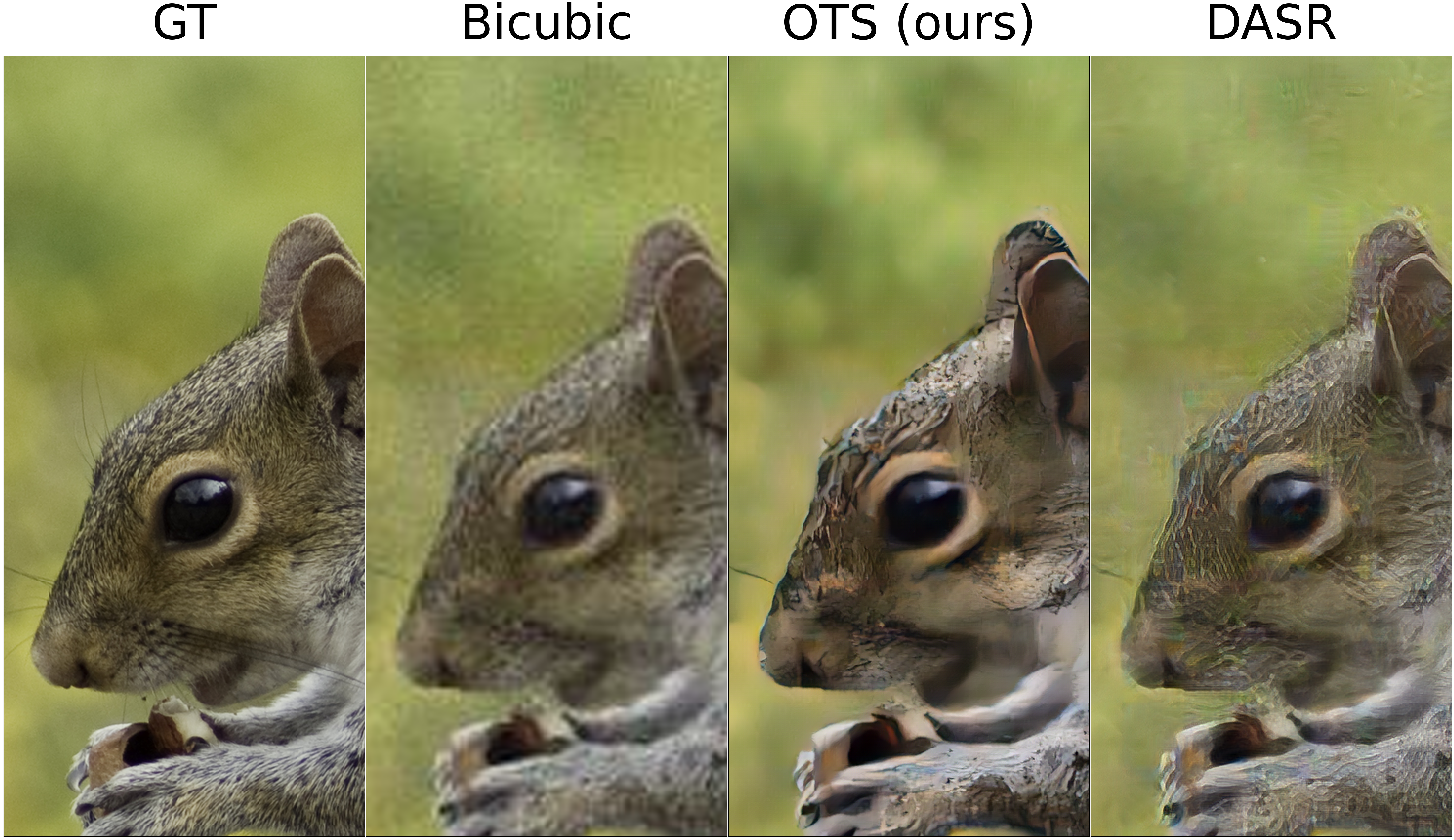
Figure 1: Super-resolution of a squirrel using Bicubic upsample, OTS (ours) and DASR (Wei et al., 2021) methods (4$\times$4 upsample, 370$\times$800 crops).

The problem of image super-resolution (SR) is to reconstruct a high-resolution (HR) image from its low-resolution (LR) counterpart. In many modern deep learning approaches, SR networks are trained in a supervised manner by using synthetic datasets containing LR-HR pairs (Lim et al., 2017, 4.1); (Zhang et al., 2018b, 4.1). For example, it is common to create LR images from HR with a simple downscaling, e.g., bicubic (Ledig et al., 2017, 3.2). However, such an artificial setup barely represents the practical setting, in which the degradation is more sophisticated and unknown (Maeda, 2020). This obstacle suggests the necessity of developing methods capable of learning SR maps from unpaired data without considering prescribed degradations.

Contributions. We study the unpaired image SR task and its solutions based on Generative Adversarial Networks (Goodfellow et al., 2014, GANs) and analyse them from the Optimal Transport (OT, see (Villani, 2008)) perspective.

1. We investigate the GAN optimization objectives regularized with content losses, which are common in unpaired image SR methods (5, 4). We prove that the solution to such objectives is always an optimal transport map. We theoretically and empirically show that such maps are biased (7.1), i.e., they do not transform the LR image distribution to the true HR image distribution.

2. We provide an algorithm to fit an unbiased OT map for perceptual transport cost (6.1) and apply it to the unpaired image SR problem (7.2). We establish connections between our algorithm and regularized GANs using integral probability metrics (IPMs) as a loss (6.2).

Our algorithm solves a minimax optimization objective and does not require extensive hyperparameter search, which makes it different from the existing methods for unpaired image SR. At the same time, the algorithm provides a nearly state-of-art performance in the unpaired image SR problem (7.2).

Notation. We use $\mathcal{X},\mathcal{Y}$ to denote Polish spaces and $\mathcal{P}(\mathcal{X}),\mathcal{P}(\mathcal{Y})$ to denote the respective sets of probability distributions on them. We denote by $\Pi(\mathbb{P},\mathbb{Q})$ the set of probability distributions on $\mathcal{X}\times\mathcal{Y}$ with marginals $\mathbb{P}$ and $\mathbb{Q}$. For a measurable map $T:\mathcal{X}\rightarrow\mathcal{Y}$, we denote the associated push-forward operator by $T_{\#}$. The expression $\|\cdot\|$ denotes the usual Euclidean norm if not stated otherwise. We denote the space of $\mathbb{Q}$-integrable functions on $\mathcal{Y}$ by $L^{1}(\mathbb{Q})$.

2 Unpaired Image Super-Resolution Task

In this section, we formalize the unpaired image super-resolution task that we consider (Figure 2).

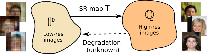
Figure 2: The task of super-resolution we consider.

Let $\mathbb{P}$ and $\mathbb{Q}$ be two distributions of LR and HR images, respectively, on spaces $\mathcal{X}$ and $\mathcal{Y}$, respectively. We assume that $\mathbb{P}$ is obtained from $\mathbb{Q}$ via some unknown degradation. The learner has access to unpaired random samples from $\mathbb{P}$ and $\mathbb{Q}$. The task is to fit a map ${T:\mathcal{X}\rightarrow\mathcal{Y}}$ satisfying ${T_{\#}\mathbb{P}=\mathbb{Q}}$ which inverts the degradation.

We highlight that the image SR task is theoretically ill-posed for two reasons.

1. Non-existence. The degradation filter may be non-injective and, consequently, non-invertible. This is a theoretical obstacle to learn one-to-one SR maps $T$.

2. Ambiguity. There might exist multiple maps satisfying ${T_{\#}\mathbb{P}=\mathbb{Q}}$ but only one inverting the degradation. With no prior knowledge about the correspondence between $\mathbb{P}$ and $\mathbb{Q}$, it is unclear how to pick this particular map.

The first issue is usually not taken into account in practice. Most existing paired and unpaired SR methods learn one-to-one SR maps $T$, see (Ledig et al., 2017; Lai et al., 2017; Wei et al., 2021).

The second issue is typically softened by regularizing the model with the content loss. In the real-world, it is reasonable to assume that HR and the corresponding LR images are close. Thus, the fitted SR map $T$ is expected to only slightly change the input image. Formally, one may require the learned map $T$ to have the small value of

$$\mathcal{R}_{c}(T)\stackrel{{\scriptstyle def}}{{=}}\int_{\mathcal{Y}}c\big{(}x,T(x)\big{)}d\mathbb{P}(x),$$ (1)

where $c:\mathcal{X}\times\mathcal{Y}\rightarrow\mathbb{R}_{+}$ is a function estimating how different the inputs are. The most popular example is the $\ell^{1}$ identity loss, i.e, formulation (1) for $\mathcal{X}=\mathcal{Y}=\mathbb{R}^{D}$ and $c(x,y)=\|x-y\|_{1}$.

More broadly, losses $\mathcal{R}_{c}(T)$ are typically called content losses and incorporated into training objectives of methods for SR (Lugmayr et al., 2019a, 3.4), (Kim et al., 2020, 3) and other unpaired tasks beside SR (Taigman et al., 2016, 4), (Zhu et al., 2017, 5.2) as regularizers. They stimulate the learned map $T$ to minimally change the image content.

3 Background on Optimal Transport

In this section, we give the key concepts of the OT theory (Villani, 2008) that we use in our paper.

Primal form. For two distributions ${\mathbb{P}\in\mathcal{P}(\mathcal{X})}$ and ${\mathbb{Q}\in\mathcal{P}(\mathcal{Y})}$ and a transport cost $c:\mathcal{X}\times\mathcal{Y}\rightarrow\mathbb{R}$, Monge’s primal formulation of the optimal transport cost is as follows:

$$\text{Cost}(\mathbb{P},\mathbb{Q})\stackrel{{\scriptstyle\text{def}}}{{=}}\inf_{T_{\#}\mathbb{P}=\mathbb{Q}}\ \int_{\mathcal{X}}c\big{(}x,T(x)\big{)}d\mathbb{P}(x),$$ (2)

where the minimum is taken over the measurable functions (transport maps) $T:\mathcal{X}\rightarrow\mathcal{Y}$ that map $\mathbb{P}$ to $\mathbb{Q}$, see Figure 3(a). The optimal $T^{*}$ is called the optimal transport map.

Note that (2) is not symmetric, and this formulation does not allow mass splitting, i.e., for some $\mathbb{P},\mathbb{Q}$ there may be no map $T$ that satisfies $T_{\#}\mathbb{P}=\mathbb{Q}$. Thus, (Kantorovitch, 1958) proposed the relaxation:

$$\text{Cost}(\mathbb{P},\mathbb{Q})\stackrel{{\scriptstyle\text{def}}}{{=}}\inf_{\pi\in\Pi(\mathbb{P},\mathbb{Q})}\int_{\mathcal{X}\times\mathcal{Y}}c(x,y)d\pi(x,y),$$ (3)

where the minimum is taken over the transport plans $\pi$, i.e., the measures on $\mathcal{X}\times\mathcal{Y}$ whose marginals are $\mathbb{P}$ and $\mathbb{Q}$ (Figure 3(b)). The optimal $\pi^{*}\in\Pi(\mathbb{P},\mathbb{Q})$ is called the optimal transport plan.

With mild assumptions on the transport cost $c(x,y)$ and distributions $\mathbb{P}$, $\mathbb{Q}$, the minimizer $\pi^{*}$ of (3) always exists (Villani, 2008, Theorem 4.1) but might not be unique. If $\pi^{*}$ is of the form $[\text{id},T^{*}]_{\#}\mathbb{P}\in\Pi(\mathbb{P},\mathbb{Q})$ for some $T^{*}$, then $T^{*}$ is an optimal transport map that minimizes (2).

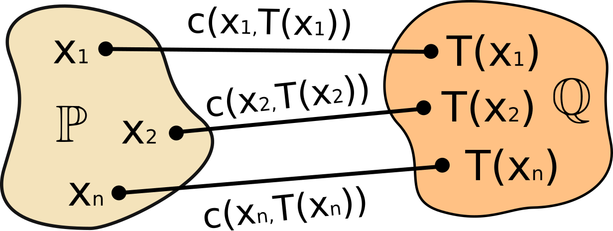
(a) Monge’s formulation of OT.

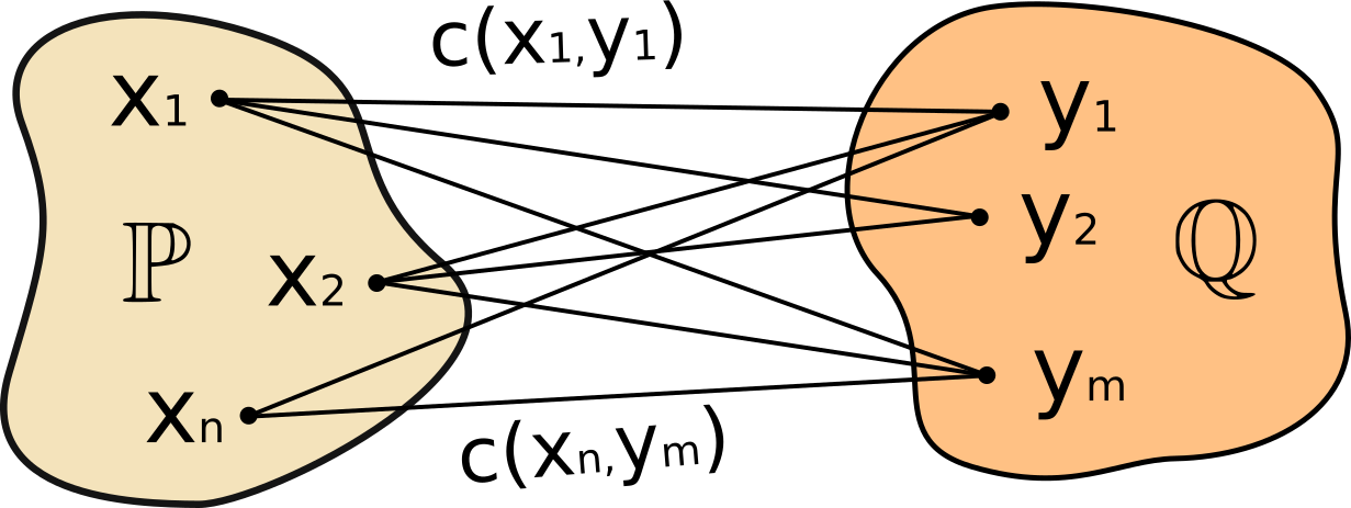
(b) Kantorovich’s formulation of OT.

Figure 3: Monge’s and Kantorovich’s formulations of Optimal Transport.

Dual form. The dual form (Villani, 2003) of OT cost (3) is as follows:

$$\text{Cost}(\mathbb{P},\mathbb{Q})=\sup_{f}\bigg{[}\int_{\mathcal{X}}f^{c}(x)d\mathbb{P}(x)+\int_{\mathcal{Y}}f(y)d\mathbb{Q}(y)\bigg{]};$$ (4)

here $\sup$ is taken over all $f\!\in\!\mathcal{L}^{1}(\mathbb{Q})$, and ${f^{c}(x)\!=\!\inf\limits_{y\in\mathcal{Y}}\!\big{[}c(x,y)\!-\!f(y)\!\big{]}}$ is the $c$-transform of $f$.

4 Related Work

Unpaired Image Super-Resolution. Existing approaches to unpaired image SR mainly solve the problem in two steps. One group of approaches learn the degradation operation at the first step and then train a super-resolution model in a supervised manner using generated pseudo-pairs, see (Bulat et al., 2018; Fritsche et al., 2019). Another group of approaches (Yuan et al., 2018; Maeda, 2020) firstly learn a mapping from real-world LR images to “clean” LR images, i.e., HR images, downscaled using predetermined (e.g., bicubic) operation, and then a mapping from “clean" LR to HR images. Most methods are based on CycleGAN (Zhu et al., 2017), initially designed for the domain transfer task, and utilize cycle-consistency loss. Methods are also usually endowed with several other losses, e.g. content (Kim et al., 2020, 3), identity (Wang et al., 2021, 3.2) or perceptual (Ji et al., 2020, 3.4).

Optimal Transport in Generative Models. The majority of existing OT-based generative models employ OT cost as the loss function to update the generative network, e.g., see (Arjovsky et al., 2017). These methods are out of scope of the present paper, since they do not compute OT maps. Existing methods to compute the OT map approach the primal (2), (3) or dual form (4). Primal-form methods (Lu et al., 2020; Xie et al., 2019; Bousquet et al., 2017; Balaji et al., 2020) optimize complex GAN objectives such as (5) and provide biased solutions (5, 7.1). For a comprehensive overview of dual-form methods, we refer to (Korotin et al., 2021). The authors conduct an evaluation of OT methods for the quadratic cost $c(x,y)=\|x-y\|^{2}$. According to them, the best performing method is $\lfloor\text{MM:R}\rceil$. It is based on the variational reformulation of (4), which is a particular case of our formulation (12). Extensions of $\lfloor\text{MM:R}\rceil$ appear in (Rout et al., 2022; Fan et al., 2021).

5 Biased Optimal Transport in GANs

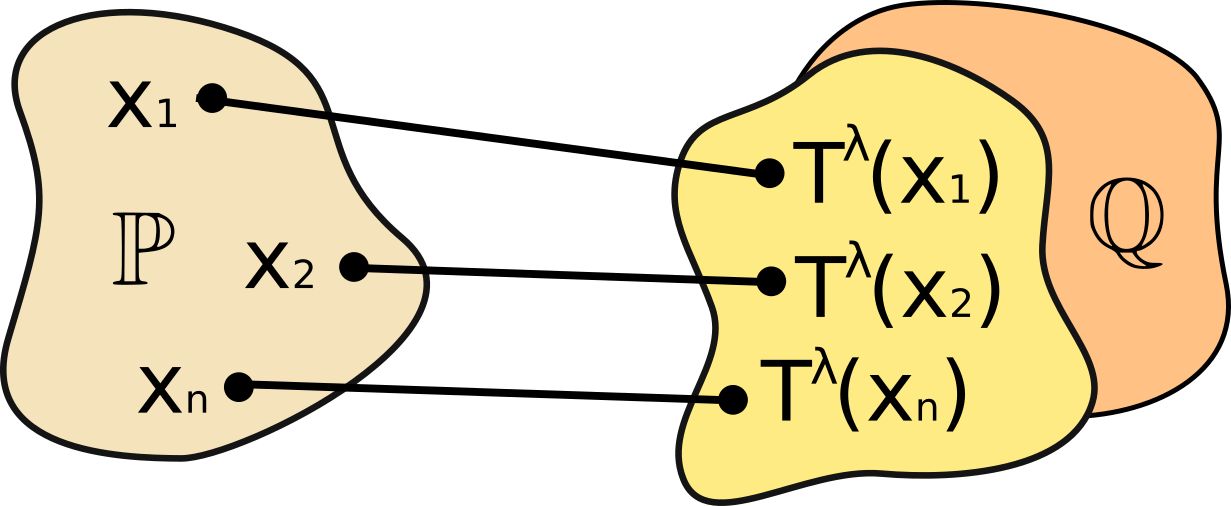
Figure 4: Illustration of Lemma 1. The solution $T^{\lambda}$ of (5) is an OT map from $\mathbb{P}$ to $T^{\lambda}_{\#}\mathbb{P}$. In general, $T^{\lambda}_{\#}\mathbb{P}\neq\mathbb{Q}$ (Thm. 1).

In this section, we establish connections between GAN methods regularized by content losses (1) and OT. A common approach to solve the unpaired SR via GANs is to define a loss function $\mathcal{D}:\mathcal{P}(\mathcal{Y})\times\mathcal{P}(\mathcal{Y})\rightarrow\mathbb{R}_{+}$ and train a generative neural network $T$ via minimizing

$$\inf_{T:\mathcal{X}\mapsto\mathcal{Y}}\big{[}\mathcal{D}(T_{\#}\mathbb{P},\mathbb{Q})+\lambda\mathcal{R}_{c}(T)\big{]}.$$ (5)

The term $\mathcal{D}(T_{\#}\mathbb{P},\mathbb{Q})$ ensures that the generated distribution $T_{\#}\mathbb{P}$ of SR images is close to the true HR distribution $\mathbb{Q}$; the second term $\mathcal{R}_{c}(T)$ is the content loss (1). For convenience, we assume that $\mathcal{D}(\mathbb{Q},\mathbb{Q})=0$ for all $\mathbb{Q}\in\mathcal{P(Y)}$. Two most popular examples of $\mathcal{D}$ are the Jensen–Shannon divergence (Goodfellow et al., 2014), i.e., the vanilla GAN loss, and the Wasserstein-1 loss (Arjovsky & Bottou, 2017). In unpaired SR methods, the optimization objectives are typically more complicated than (5). In addition to the content or identity loss (1), several other regularizations are usually introduced, see 4.

For a theoretical analysis, we stick to the basic formulation regularized with generic content loss (5). It represents the simplest and straightforward SR setup. We prove the following lemma, which connects the solution $T^{\lambda}$ of (5) and optimal maps for transport cost $c(x,y)$.

Lemma 1 (The solution of the regularized GAN is an OT map).

Assume that $\lambda>0$ and the minimizer $T^{\lambda}$ of (5) exists. Then $T^{\lambda}$ is an OT map between $\mathbb{P}$ and $\mathbb{Q}^{\lambda}\stackrel{{\scriptstyle\text{def}}}{{=}}T^{\lambda}_{\#}\mathbb{P}$ for cost $c(x,y)$, i.e., it minimizes

$$\inf_{T_{\#}\mathbb{P}=\mathbb{Q}^{\lambda}}\mathcal{R}_{c}(T)=\inf_{T_{\#}\mathbb{P}=\mathbb{Q}^{\lambda}}\int_{\mathcal{X}}c\big{(}x,T(x)\big{)}d\mathbb{P}(x).$$

Proof.

Assume that $T^{\lambda}$ is not an optimal map between $\mathbb{P}$ and $T^{\lambda}_{\#}\mathbb{P}$. Then there exists a more optimal $T^{\dagger}$ satisfying ${T^{\dagger}_{\#}\mathbb{P}=T_{\#}^{\lambda}\mathbb{P}}$ and $\mathcal{R}_{c}(T^{\dagger})<\mathcal{R}_{c}(T^{\lambda})$. We substitute this $T^{\dagger}$ to (5) and derive

$$\mathcal{D}(T^{\dagger}_{\#}\mathbb{P},\mathbb{Q})+\lambda\mathcal{R}_{c}(T^{\dagger})=\mathcal{D}(T^{\lambda}_{\#}\mathbb{P},\mathbb{Q})+\lambda\mathcal{R}_{c}(T^{\dagger})<\mathcal{D}(T^{\lambda}_{\#}\mathbb{P},\mathbb{Q})+\lambda\mathcal{R}_{c}(T^{\lambda}),$$

which is a contradiction, since $T^{\lambda}$ is a minimizer of (5), but $T^{\dagger}$ provides the smaller value. ∎

Our Lemma 1 states that the minimizer $T^{\lambda}$ of a regularized GAN problem is always an OT map between $\mathbb{P}$ and the distribution $\mathbb{Q}^{\lambda}$ generated by the same $T^{\lambda}$ from $\mathbb{P}$. However, below we prove that $\mathbb{Q}^{\lambda}\neq\mathbb{Q}$, i.e., $T^{\lambda}$ does not actually produce the distribution of HR images (Figure 4). To begin with, we state and prove the following auxiliary result.

Lemma 2 (Reformulation of the regularized GAN via distributions).

Under the assumptions of Lemma 1, let $\mathcal{X}=\mathcal{Y}$ be a compact subset of $\mathbb{R}^{D}$ with negligible boundary. Let $\mathbb{P}\!\in\!\mathcal{P(X)}$ be absolutely continuous, $\mathbb{Q}\!\in\!\mathcal{P(Y)}$ and $c(x,y)\!=\!\|x-y\|^{p}$ with $p>1$. Then (5) is equivalent to

$$\inf_{\mathbb{Q}^{\prime}\in\mathcal{P}(\mathcal{Y})}\mathcal{F}(\mathbb{Q}^{\prime})\stackrel{{\scriptstyle\text{{def}}}}{{=}}\!\inf_{\mathbb{Q}^{\prime}\in\mathcal{P}(\mathcal{Y})}\big{[}\mathcal{D}(\mathbb{Q}^{\prime},\mathbb{Q})+\lambda\cdot\text{{Cost}}(\mathbb{P},\mathbb{Q}^{\prime})\big{]},$$ (6)

and the solutions of (5) and (6) are related as $\mathbb{Q}^{\lambda}=T^{\lambda}_{\#}\mathbb{P}$, where $\mathbb{Q}^{\lambda}$ is the minimizer of (6).

Proof.

We derive

$$\inf_{T:\mathcal{X}\mapsto\mathcal{Y}}\big{[}\mathcal{D}(T_{\#}\mathbb{P},\mathbb{Q})+\lambda\mathcal{R}_{c}(T)\big{]}=\inf_{T:\mathcal{X}\mapsto\mathcal{Y}}\big{[}\mathcal{D}(T_{\#}\mathbb{P},\mathbb{Q})+\lambda\int_{\mathcal{X}}c\big{(}x,T(x)\big{)}d\mathbb{P}(x)\big{]}=$$ (7)

$$\inf_{T:\mathcal{X}\mapsto\mathcal{Y}}\big{[}\mathcal{D}(T_{\#}\mathbb{P},\mathbb{Q})+\lambda\cdot\text{Cost}(\mathbb{P},T_{\#}\mathbb{P})\big{]}=\inf_{\mathbb{Q}^{\prime}\in\mathcal{P}(\mathcal{Y})}\big{[}\mathcal{D}(\mathbb{Q}^{\prime},\mathbb{Q})+\lambda\cdot\text{Cost}(\mathbb{P},\mathbb{Q}^{\prime})\big{]}.\vspace{-2mm}$$ (8)

In transition from (7) to (8), we use the definition of OT cost (2) and our Lemma 1, which states that the minimizer $T^{\lambda}$ of (5) is an OT map, i.e., $\int_{\mathcal{X}}c\big{(}x,T^{\lambda}(x)\big{)}d\mathbb{P}(x)=\text{Cost}(\mathbb{P},T^{\lambda}_{\#}\mathbb{P})$. The equality in (8) follows from the fact that $\mathbb{P}$ is abs. cont. and $c(x,y)=\|x-y\|^{p}$: for all $\mathbb{Q}^{\prime}\in\mathcal{P}(\mathcal{Y})$ there exists a (unique) solution $T$ to the Monge OT problem (2) for $\mathbb{P},\mathbb{Q}^{\prime}$ (Santambrogio, 2015, Thm. 1.17). ∎

In the following Theorem, we prove that, in general, $\mathbb{Q}^{\lambda}\neq\mathbb{Q}$ for the minimizer $\mathbb{Q}^{\lambda}$ of (6).

Theorem 1 (The distribution solving the regularized GAN problem is always biased).

Under the assumptions of Lemma 2, assume that the first variation (Santambrogio, 2015, Definition 7.12) of the functional ${\mathbb{Q}^{\prime}\mapsto\mathcal{D}(\mathbb{Q}^{\prime},\mathbb{Q})}$ at the point $\mathbb{Q}^{\prime}=\mathbb{Q}$ exists and is equal to zero. This means that $\mathcal{D}(\mathbb{Q}+\epsilon\Delta\mathbb{Q})=\mathcal{D}(\mathbb{Q},\mathbb{Q})+o(\epsilon)$ for every signed measure $\Delta\mathbb{Q}$ of zero total mass and $\epsilon\geq 0$ such that $\mathbb{Q}+\epsilon\Delta\mathbb{Q}\in\mathcal{P}(\mathcal{Y})$. Then, if $\mathbb{P}\neq\mathbb{Q}$, then $\mathbb{Q}^{\prime}=\mathbb{Q}$ does not deliver the minimum to $\mathcal{F}$.

Before proving Theorem 1, we highlight that the assumption about the vanishing first variation of $\mathbb{Q}^{\prime}\mapsto\mathcal{D}(\mathbb{Q}^{\prime},\mathbb{Q})$ at $\mathbb{Q}^{\prime}=\mathbb{Q}$ is reasonable. In Appendix A, we prove that this assumption holds for the popular GAN discrepancies $\mathcal{D}(\mathbb{Q}^{\prime},\mathbb{Q})$, e.g., $f$-divergences (Nowozin et al., 2016), Wasserstein distances (Arjovsky et al., 2017), and Maximum Mean Discrepancies (Li et al., 2017).

Proof.

Let $\Delta\mathbb{Q}=\mathbb{P}-\mathbb{Q}$ denote the difference measure of $\mathbb{P}$ and $\mathbb{Q}$. It has zero total mass and $\forall\epsilon\in[0,1]$ it holds that $\mathbb{Q}+\epsilon\Delta\mathbb{Q}=\epsilon\mathbb{P}+(1-\epsilon)\mathbb{Q}$ is a mixture distribution of probability distributions $\mathbb{P}$ and $\mathbb{Q}$. As a result, for all $\epsilon\in[0,1]$, we have

$$\mathcal{F}(\mathbb{Q}+\epsilon\Delta\mathbb{Q})=\mathcal{D}(\mathbb{Q}+\epsilon\Delta\mathbb{Q},\mathbb{Q})+\lambda\cdot\text{Cost}(\mathbb{P},\mathbb{Q}+\epsilon\Delta\mathbb{Q})$$

$$=\mathcal{D}(\mathbb{Q},\mathbb{Q})+o(\epsilon)+\lambda\cdot\text{Cost}(\mathbb{P},\epsilon\mathbb{P}+(1-\epsilon)\mathbb{Q})$$ (9)

$$\leq o(\epsilon)+\lambda\cdot\epsilon\cdot\text{Cost}(\mathbb{P},\mathbb{P})+\lambda\cdot(1-\epsilon)\cdot\text{Cost}(\mathbb{P},\mathbb{Q})=o(\epsilon)+\lambda\cdot(1-\epsilon)\cdot\text{Cost}(\mathbb{P},\mathbb{Q})$$ (10)

$$=\underbrace{\lambda\cdot\text{Cost}(\mathbb{P},\mathbb{Q})}_{=\mathcal{F}(\mathbb{Q})}-\lambda\cdot\epsilon\cdot\underbrace{\text{Cost}(\mathbb{P},\mathbb{Q})}_{>0}+o(\epsilon),$$

where in transition from (9) to (10), we use $\mathcal{D}(\mathbb{Q},\mathbb{Q})=0$ and exploit the convexity of the OT cost (Villani, 2003, Theorem 4.8). In (10), we use $\text{Cost}(\mathbb{P},\mathbb{P})=0$. We see that $\mathcal{F}(\mathbb{Q}\!+\!\epsilon\Delta\mathbb{Q})$ is smaller then $\mathcal{F}(\mathbb{Q})$ for sufficiently small $\epsilon>0$, i.e., $\mathbb{Q}^{\prime}\!=\!\mathbb{Q}$ does not minimize $\mathcal{F}$. ∎

Corollary 1.

Under the assumptions of Theorem 1, the solution $T^{\lambda}$ of regularized GAN (5) is biased, i.e., it does not satisfy $T^{\lambda}_{\#}\mathbb{P}=\mathbb{Q}$ and does not transform LR images to true HR ones.

Additionally, we provide a toy example that further illustrates the issue with the bias.

Example 1.

Consider $\mathcal{X}=\mathcal{Y}=\mathbb{R}^{1}$. Let $\mathbb{P}=\frac{1}{2}\delta_{0}+\frac{1}{2}\delta_{2}$, $\mathbb{Q}=\frac{1}{2}\delta_{1}+\frac{1}{2}\delta_{3}$ be distributions concentrated at $\{0,2\}$ and $\{1,3\}$, respectively. Put $c(x,y)=|x-y|$ to be the content loss. Also, let $\mathcal{D}$ to be the OT cost for $|x-y|^{2}$. Then for $\lambda=0$ there exist two maps between $\mathbb{P}$ and $\mathbb{Q}$ that deliver the same minimal value for (5), namely $T(0)=1,T(2)=3$ and $T(0)=3,T(2)=1$. For $\lambda>0$, the optimal solution of the problem (5) is unique, biased and given by $T(0)=1-\frac{\lambda}{2},T(2)=3-\frac{\lambda}{2}$.

Proof.

Let $T(0)=t_{0}$ and $T(2)=t_{2}$. Then $T_{\#}\mathbb{P}=\frac{1}{2}\delta_{t_{0}}+\frac{1}{2}\delta_{t_{2}}$, and now (5) becomes

$$\min_{t_{0},t_{2}}\bigg{[}\min\big{\{}\frac{1}{2}(t_{0}-1)^{2}+\frac{1}{2}(t_{2}-3)^{2};\frac{1}{2}(t_{0}-3)^{2}+\frac{1}{2}(t_{2}-1)^{2}\big{\}}+\lambda\big{\{}\frac{1}{2}|0-t_{0}|+\frac{1}{2}|2-t_{2}|\big{\}}\bigg{]},$$

where the second term is $\mathcal{R}_{c}(T)$ and the first term is the OT cost $\mathcal{D}(T_{\#}\mathbb{P},\mathbb{Q})$ expressed as the minimum over the transport costs of two possible transport maps $t_{0}\mapsto 1;t_{2}\mapsto 3$ and $t_{0}\mapsto 3;t_{2}\mapsto 1$. The minimizer can be derived analytically and equals $t_{0}=1-\frac{\lambda}{2},t_{2}=3-\frac{\lambda}{2}$. ∎

In Example 1, $T_{\#}^{\lambda}\mathbb{P}=\mathbb{Q}^{\lambda}$ never matches $\mathbb{Q}$ exactly for $\lambda>0$. In 7.1, we conduct an evaluation of maps obtained via minimizing objective (5) on the synthetic benchmark by (Korotin et al., 2021). We empirically demonstrate that the bias exists and it is indeed a notable practical issue.

Remarks. Throughout this section, we enforce additional assumptions on (5), e.g., we restrict our analysis to content losses $c(\cdot,\cdot)$, which are powers of Euclidean norms $\|\cdot\|^{p}$. This is needed to make the derivations concise and to be able to exploit the available results in OT. We think that the provided results hold under more general assumptions and leave this question open for future studies.

6 Unbiased Optimal Transport Solver

In 6.1, we derive our algorithm to compute OT maps. Importantly, in 6.2, we detail its differences and similarities with regularized GANs, which we discussed in 5.

6.1 Minimax Optimization Algorithm

We derive a minimax optimization problem to recover the optimal transport map from $\mathbb{P}$ to $\mathbb{Q}$. We expand the dual form (4). To do this, we first note that

$$\int_{\mathcal{X}}f^{c}(x)d\mathbb{P}(x)=\int_{\mathcal{X}}\inf_{y\in\mathcal{Y}}\left\{c(x,y)-f(y)\right\}d\mathbb{P}(x)=\inf_{T:\mathcal{X}\rightarrow\mathcal{Y}}\int_{\mathcal{X}}\left\{c\big{(}x,T(x)\big{)}-f\big{(}T(x)\big{)}\right\}d\mathbb{P}(x).$$ (11)

Here we replace the optimization over points $y\in\mathcal{Y}$ with an equivalent optimization over the functions ${T:\mathcal{X}\rightarrow\mathcal{Y}}$. This is possible due to the Rockafellar interchange theorem (Rockafellar, 1976, Theorem 3A). Substituting (11) to (4), we have

$$\text{Cost}(\mathbb{P},\mathbb{Q})=\sup_{f}\inf_{T:\mathcal{X}\rightarrow\mathcal{Y}}\bigg{[}\int_{\mathcal{Y}}f(y)d\mathbb{Q}(y)+\int_{\mathcal{X}}\left\{c\big{(}x,T(x)\big{)}-f\big{(}T(x)\big{)}\right\}d\mathbb{P}(x)\bigg{]}\vspace{-1.7mm}$$ (12)

We denote the expression under the $\sup\inf$ by $\mathcal{L}(f,T)$. Now we show that by solving the saddle point problem (12) one can obtain the OT map $T^{*}$.

Lemma 3 (OT maps solve the saddle point problem).

Assume that the OT map $T^{*}$ between $\mathbb{P},\mathbb{Q}$ for cost $c(x,y)$ exists. Then, for every optimal potential $f^{*}\in\operatorname*{arg\,sup}_{f}\big{[}\inf_{T:\mathcal{X}\rightarrow\mathcal{Y}}\mathcal{L}(f,T)\big{]}$ of (12),

$$T^{*}\in\operatorname*{arg\,inf}_{T:\mathcal{X}\rightarrow\mathcal{Y}}\int_{\mathcal{X}}\left\{c\big{(}x,T(x)\big{)}-f\big{(}T(x)\big{)}\right\}d\mathbb{P}(x).$$ (13)

Proof.

Since $f^{*}$ is optimal, we have $\inf_{T:\mathcal{X}\rightarrow\mathcal{Y}}\mathcal{L}(f^{*},T)=\text{Cost}(\mathbb{P},\mathbb{Q}).$ We use $T^{*}_{\#}\mathbb{P}=\mathbb{Q}$ and the change of variables $y=T^{*}(x)$ to derive $\int_{\mathcal{X}}f^{*}\big{(}T^{*}(x)\big{)}d\mathbb{P}=\int_{\mathcal{Y}}f^{*}(y)d\mathbb{Q}$. Substituting this equality into (12), we obtain $\mathcal{L}(f^{*},T^{*})=\int_{\mathcal{X}}c\big{(}x,T^{*}(x)\big{)}d\mathbb{P}(x)=\text{Cost}(\mathbb{P},\mathbb{Q}),$ i.e., (13) holds. ∎

Lemma 13 states that one can solve a saddle point problem (12), obtain an optimal pair $(f^{*},T^{*})$, and use $T^{*}$ as an OT map from $\mathbb{P},\mathbb{Q}$. For general $\mathbb{P},\mathbb{Q}$, the $\operatorname*{arg\,inf}_{T}$ set for an optimal $f^{*}$ might contain not only OT map $T^{*}$ but other functions as well. However, our experiments (7) show that this is not a serious issue in practice. To solve the optimization problem (12), we approximate the potential $f$ and map $T$ with neural networks $f_{\omega}$ and $T_{\theta}$, respectively. We train the networks with stochastic gradient ascent-descent by using random batches from $\mathbb{P},\mathbb{Q}$.

The practical optimization procedure is detailed in Algorithm 1. We call this procedure an Optimal Transport Solver (OTS).

Input : distributions $\mathbb{P},\mathbb{Q}$ accessible by samples; mapping network $T_{\theta}:\mathcal{X}\rightarrow\mathcal{Y}$;

potential $f_{\omega}:\mathcal{X}\rightarrow\mathbb{R}$; transport cost $c:\mathcal{X}\times\mathcal{Y}\rightarrow\mathbb{R}$; number $K_{T}$ of inner iters;

Output : approximate OT map $(T_{\theta})_{\#}\mathbb{P}\approx\mathbb{Q}$;

repeat

     Sample batches $X\sim\mathbb{P}$, $Y\!\sim\!\mathbb{Q}$;

     $\mathcal{L}_{f}\leftarrow\frac{1}{|X|}\sum\limits_{x\in X}f_{\omega}\big{(}T_{\theta}(x)\big{)}-\frac{1}{|Y|}\sum\limits_{y\in Y}f_{\omega}(y)$;

     Update $\omega$ by using $\frac{\partial\mathcal{L}_{v}}{\partial\omega}$;

    

    for $k_{T}=1,2,\dots,K_{T}$ do

         Sample batch $X\sim\mathbb{P}$;

         ${\mathcal{L}_{T}=\frac{1}{|X|}\sum\limits_{x\in X}\big{[}c\big{(}x,T_{\theta}(x)\big{)}-f_{\omega}\big{(}T_{\theta}(x)\big{)}\big{]}}$;

         Update $\theta$ by using $\frac{\partial\mathcal{L}_{T}}{\partial\theta}$;

        

    

until not converged;

Algorithm 1 OT solver to compute the OT map between $\mathbb{P}$ and $\mathbb{Q}$ for transport cost $c(x,y)$.

6.2 Regularized GANs vs. Optimal Transport Solver

In this subsection, we discuss similarities and differences between our optimization objective (12) and the objective of regularized GANs (5). We establish an intriguing connection between GANs that use integral probability metrics (IPMs) as $\mathcal{D}$. A discrepancy $\mathcal{D}\!:\!\mathcal{P}(\mathcal{Y})\!\times\!\mathcal{P}(\mathcal{Y})\!\rightarrow\!\mathbb{R}_{+}$ is an IPM if

$$\mathcal{D}(\mathbb{Q}_{1},\mathbb{Q}_{2})\!=\!\sup_{f\in\mathcal{F}}\!\big{[}\!\int_{\mathcal{Y}}\!f(y)d\mathbb{Q}_{2}(y)\!-\!\int_{\mathcal{Y}}\!f(y)d\mathbb{Q}_{1}(y)\big{]}\!,\vspace{-1.8mm}$$ (14)

where the maximization is performed over some certain class $\mathcal{F}$ of functions (discriminators) ${f:\mathcal{Y}\rightarrow\mathbb{R}}$. The most popular example of $\mathcal{D}$ is the Wasserstein-1 loss (Arjovsky & Bottou, 2017), where $\mathcal{F}$ is a class of $1$-Lipschitz functions. For other IPMs, see (Mroueh et al., 2017, Table 1).

Substituting (14) to (5) yields the saddle-point optimization problem for the regularized IPM GAN:

$$\inf_{T:\mathcal{X}\rightarrow\mathcal{Y}}\bigg{[}\sup_{f\in\mathcal{F}}\left\{\!\int_{\mathcal{Y}}\!f(y)d\mathbb{Q}(y)\!-\!\int_{\mathcal{X}}\!f\big{(}T(x)\big{)}d\mathbb{P}(x)\right\}+\lambda\int_{\mathcal{X}}c\big{(}x,T(x)\big{)}d\mathbb{P}(x)\}\bigg{]}$$

$$=\inf_{T:\mathcal{X}\rightarrow\mathcal{Y}}\sup_{f\in\mathcal{F}}\bigg{[}\int_{\mathcal{Y}}f(y)d\mathbb{Q}(y)+\int_{\mathcal{X}}\left\{\lambda\cdot c\big{(}x,T(x)\big{)}-f\big{(}T(x)\big{)}\right\}d\mathbb{P}(x)\bigg{]}.\vspace{-3.0mm}$$ (15)

We emphasize that the expression inside (15) for $\lambda=1$ is similar to the expression in OTS optimization (12). Below we highlight the key differences between (12) and (15).

First, in OTS the map $T$ is a solution to the inner optimization problem, while in IPM GAN the generator $T$ is a solution to the outer problem. Swapping $\inf_{T}$ and $\sup_{f}$ is prohibited and, in general, yields a different problem, e.g., $1\!=\!\inf_{x}\sup_{y}\cos(x\!+\!y)\neq\sup_{y}\inf_{x}\cos(x\!+\!y)\!=\!-\!1$.

Second, in OTS the optimization over potential $f$ is unconstrained, while in IPM GAN it must belong to $\mathcal{F}$, some certain restricted class of functions. For example, when ${\mathcal{D}}$ is the Wasserstein-1 ($\mathbb{W}_{1}$) IPM, one has to use an additional penalization, e.g., the gradient penalty (Gulrajani et al., 2017). This further complicates the optimization and adds hyperparameters which have to be carefully selected.

Third, the optimization of IPM GAN requires selecting a parameter $\lambda$ that balances the content loss $\mathcal{R}_{c}$ and the discrepancy $\mathcal{D}$. In OTS for all costs $\lambda\cdot c(x,y)$ with $\lambda>0$, the OT map $T^{*}$ is the same.

To conclude, even for $\lambda=1$, the IPM GAN problem does not match that of OTS. Table 1 summarizes the differences and thesimilarities between OTS and regularized IPM GANs.

	Optimal Transport Solver (Ours)	Regularized IPM GAN
Minimax optimization objective	$\sup\limits_{f}\inf\limits_{T:\mathcal{X}\rightarrow\mathcal{Y}}\bigg{[}\int_{\mathcal{Y}}f(y)d\mathbb{Q}(y)+$ $\int_{\mathcal{X}}\left\{c\big{(}x,T(x)\big{)}-f\big{(}T(x)\big{)}\right\}d\mathbb{P}(x)\bigg{]}$	$\inf\limits_{T:\mathcal{X}\rightarrow\mathcal{Y}}\sup\limits_{f\in\mathcal{F}}\bigg{[}\int_{\mathcal{Y}}f(y)d\mathbb{Q}(y)+$ $\int_{\mathcal{X}}\left\{\lambda\cdot c\big{(}x,T(x)\big{)}-f\big{(}T(x)\big{)}\right\}d\mathbb{P}(x)\bigg{]}$
Transport map $T$ (generator)	$T^{*}$ solves the inner problem (for optimal $f^{*}$); it is an OT map from $\mathbb{P}$ to $\mathbb{Q}$ (Lemma 13)	$T^{*}$ solves the outer problem; it is a biased OT map (5, 7.1)
Potential $f$ (discriminator)	Unconstrained $f\in L^{1}(\mathbb{Q})$	Constrained $f\in\mathcal{F}\subset L^{1}(\mathbb{Q})$ A method to impose the constraint is needed.
Regularization weight $\lambda$	N/A	Hyperparameter choice required

Table 1: Comparison of the optimization objectives of OTS (ours) and regularized IPM GAN.

7 Evaluation

In 7.1, we assess the bias of regularized IPM GANs by using the Wasserstein-2 benchmark (Korotin et al., 2021). In 7.2, we evaluate our method on the large-scale unpaired AIM-19 dataset from (Lugmayr et al., 2019b). In Appendix D, we test it on the CelebA dataset (Liu et al., 2015). The code is written in PyTorch. We list the hyperparameters for Algorithm 1 in Table 4 of Appendix C.

Neural network architectures. We use WGAN-QC’s (Liu et al., 2019) ResNet (He et al., 2016) architecture for the potential $f_{\omega}$. In 7.1, where input and output images have the same size, we use UNet (Ronneberger et al., 2015) as a transport map $T_{\theta}$. In 7.2, the LR input images are $4\times 4$ times smaller than HR, so we use EDSR network (Lim et al., 2017).

Transport costs. In 7.1, we use the mean squared error (MSE), i.e., ${c(x,y)=\frac{\|x-y\|^{2}}{\dim(\mathcal{Y})}}$. It is equivalent to the quadratic cost but is more convenient due to the normalization. In 7.2, we consider $c(x,y)=b(\text{Up}(x),y)$, where $b$ is a cost between the bicubically upsampled LR image $x^{\text{up}}=\text{Up}(x)$ and HR image $y$. We test $b$ defined as MSE and the perceptual cost using features of a pre-trained VGG-16 network (Simonyan & Zisserman, 2014), see Appendix C for details.

7.1 Assessing the Bias in Regularized GANs

In this section, we empirically confirm the insight of 5 that the solution $T^{\lambda}$ of (5) may not satisfy $T^{\lambda}_{\#}\mathbb{P}=\mathbb{Q}$. Note if $T^{\lambda}_{\#}\mathbb{P}=\mathbb{Q}$, then by our Lemma 1, we conclude that $T^{\lambda}\equiv T^{*}$, where $T^{*}$ is an OT map from $\mathbb{P}$ to $\mathbb{Q}$ for $c(x,y)$. Thus, to access the bias, it is reasonable to compare the learned map $T^{\lambda}$ with the ground truth OT map $T^{*}$ for $\mathbb{P}$, $\mathbb{Q}$.

For evaluation, we use the Wasserstein-2 benchmark (Korotin et al., 2021). It provides high-dimensional continuous pairs $\mathbb{P}$, $\mathbb{Q}$ with an analytically known OT map $T^{*}$ for the quadratic cost ${c(x,y)=\|x-y\|^{2}}$. We use their “Early" images benchmark pair. It simulates the image deblurring setup, i.e., $\mathcal{X}=\mathcal{Y}$ is the space of $64\times 64$ RGB images, $\mathbb{P}$ is blurry faces, $\mathbb{Q}$ is clean faces satisfying $\mathbb{Q}=T^{*}_{\#}\mathbb{P}$, where $T^{*}$ is an analytically known OT map, see the 1st and 2nd lines in Figure 5.

To quantify the learned maps from $\mathbb{P}$ to $\mathbb{Q}$, we use PSNR, SSIM, LPIPS (Zhang et al., 2018a), FID (Heusel et al., 2017) metrics. Similar to (Wei et al., 2021), we use the AlexNet-based (Krizhevsky et al., 2012) LPIPS. FID and LPIPS are practically the most important since they better correlate with the human perception of the image quality. We include PSNR, SSIM as popular evaluation metrics, but they are known to badly measure perceptual quality (Zhang et al., 2018a; Nilsson & Akenine-Möller, 2020). Due to this, higher PSNR, SSIM values do not necessarily mean better performance. We calculate metrics using scikit-image for SSIM and open source implementations for PSNR, LPIPS and FID. In this section, we additionally use the $\mathcal{L}^{2}\text{-UVP}$ (Korotin et al., 2021, 4.2) metric.

On the benchmark, we compare OTS (12) and IPM GAN (5). We use MSE as the content loss $c(x,y)$. In IPM GAN, we use the Wasserstein-1 ($\mathbb{W}_{1}$) loss with the gradient penalty ${\lambda_{\text{GP}}=10}$ (Gulrajani et al., 2017) as $\mathcal{D}$. We do $10$ discriminator updates per $1$ generator update and train the model for 15K generator updates. For fair comparison, the rest hyperparameters match those of our algorithm. We train the regularized WGAN-GP with various coefficients of content loss $\lambda\in\{0,10^{-1},\dots,10^{5}\}$ and show the learned maps $T^{\lambda}$ and the map $\hat{T}$ obtained by OTS in Figure 5.

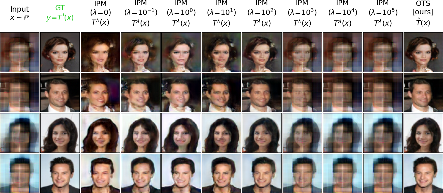
Figure 5: Comparison of OTS (ours), regularized IPM GAN on the Wasserstein-2 benchmark. The 1st line shows blurry faces $x\sim\mathbb{P}$, the 2nd line, clean faces $y=T^{*}(x)$, where $T^{*}$ is the OT map from $\mathbb{P}$ to $\mathbb{Q}$. Next lines show maps from $\mathbb{P}$ to $\mathbb{Q}$ fitted by the methods.

Metrics/ Method	Regularized IPM GAN (WGAN-GP, $\lambda_{\text{GP}}=10$)								OTS (ours)
	$\lambda=0$	$\lambda=10^{-1}$	$\lambda=10^{0}$	$\lambda=10^{1}$	$\lambda=10^{2}$	$\lambda=10^{3}$	$\lambda=10^{4}$	$\lambda=10^{5}$
$\mathcal{L}^{2}\text{-UVP}\downarrow$	$25.2\%$	$16.7\%$	$17.7\%$	$12.0\%$	$\textbf{4.0}\%$	$14.0\%$	$28.5\%$	$30.5\%$	$\textbf{1.4}\%$
FID$\downarrow$	$57.24$	$46.23$	$40.04$	$42.89$	24.25	$187.95$	$332.7$	$334.7$	$\mathbf{15.65}$
PSNR$\uparrow$	$17.90$	$19.76$	$19.34$	$20.81$	25.58	$19.91$	$16.90$	$16.52$	$\mathbf{30.02}$
SSIM$\uparrow$	$0.565$	$0.655$	$0.656$	$0.689$	0.859	$0.702$	$0.520$	$0.498$	$\mathbf{0.933}$
LPIPS$\downarrow$	$0.135$	$0.093$	$0.099$	$0.081$	0.031	$0.172$	$0.429$	$0.446$	$\mathbf{0.013}$

Table 2: Quantitative evaluation of restoration maps fitted by the regularized IPM GAN, OTS (ours) using the Wasserstein-2 images benchmark (Korotin et al., 2021).

Results. The performance of the regularized IPM GAN significantly depends on the choice of the content loss value $\lambda$. For high values $\lambda\geq 10^{3}$, the learned map is close to the identity as expected. For small values $\lambda\leq 10^{1}$, the regularization has little effect, and WGAN-GP solely struggles to fit a good restoration map. Even for the best performing $\lambda=10^{2}$ all metrics are notably worse than for OTS. Importantly, OTS decreases the burden of parameter searching as there is no parameter $\lambda$.

7.2 Large-Scale Evaluation

For evaluating our method at a large-scale, we employ the dataset by (Lugmayr et al., 2019b) of AIM 2019 Real-World Super-Resolution Challenge (Track 2). The train part contains 800 HR images with up to 2040 pixels width or height and 2650 unpaired LR images of the same shape. They are constructed using artificial, but realistic, image degradations. We quantitatively evaluate our method on the validation part of AIM dataset that contains 100 pairs of LR-HR images.

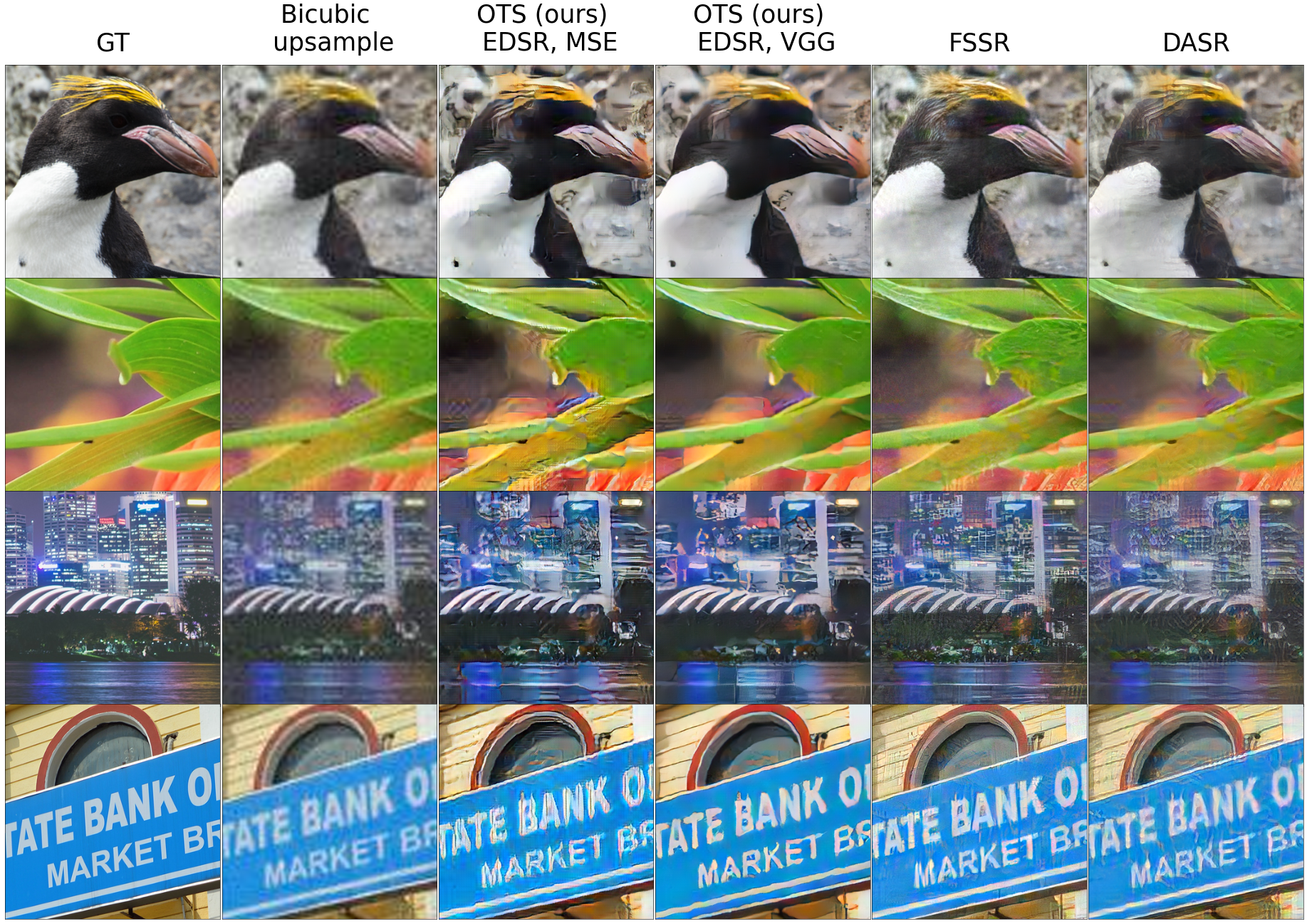
Figure 6: Qualitative results of OTS (ours), bicubic upsample, FSSR and DASR on AIM 2019 dataset (350$\times$350 crops).

Baselines. We compare OTS on AIM dataset with the bicubic upsample, FSSR (Fritsche et al., 2019) and DASR (Wei et al., 2021) methods. FSSR method is the winner of AIM 2019 Challenge; DASR is a current state-of-the-art method for unpaired image SR. Both methods utilize the idea of frequency separation and solve the problem in two steps. First, they train a network to generate LR images. Next, they train a super-resolution network using generated pseudo-pairs. Differently to FSSR, DASR also employs real-world LR images for training SR network taking into consideration the domain gap between generated and real-world LR images. Both methods utilize several losses, e.g., adversarial and perceptual, either on the entire image or on its high/low frequency components. For testing FSSR and DASR, we use their official code and pretrained models.

Implementation details. We train the networks using 128$\times$128 HR and 32$\times$32 LR random patches of images augmented via random flips and rotations. We conduct separate experiments using EDSR as the transport map and either MSE or perceptual cost.

Metrics. We calculate PSNR, SSIM, LPIPS, FID. FID is computed on $32\times 32$ patches of LR test images upsampled by the method in view w.r.t. random patches of test HR. We use 50k patches to compute FID. The other metrics are computed on the entire upsampled LR test and HR test images.

Method	FID $\downarrow$	PSNR $\uparrow$	SSIM $\uparrow$	LPIPS $\downarrow$
Bicubic upsample	178.59	22.39	0.613	0.688
OTS (ours, MSE)	139.17	19.73	0.533	0.456
OTS (ours, VGG)	89.04	20.96	0.605	0.380
FSSR	53.92	20.83	0.514	0.390
DASR	124.09	21.79	0.577	0.346

Table 3: Comparison of OTS (ours) with FSSR, DASR on AIM19 dataset. The 1st, 2nd, 3rd best results are highlighted in green, blue and underlined, respectively.

Experimental results are given in Table 3, Figure 6. The results show that the usage perceptual cost function in OTS boosts performance. According to FID, OTS with perceptual cost function beats DASR. On the other hand, it outperforms FSSR in PSNR, SSIM and, importantly, LPIPS. Note that bicubic upsample outperforms all the methods, according only to PSNR and SSIM, which have issues stated in 7.1. According to visual analysis, OTS deals better with noise artifacts. Additional results are given in Appendix E. We also demonstrate the bias issue of FSSR and DASR in Appendix B.

8 Discussion

Significance. Our analysis connects content losses in GANs with OT and reveals the bias issue. Content losses are used in a wide range of tasks besides SR, e.g., in the style transfer and domain adaptation tasks. Our results demonstrate that GAN-based methods in all these tasks may a priori lead to biased solutions. In certain cases it is undesirable, e.g., in medical applications (Bissoto et al., 2021). Failing to learn true data statistics (and learning biased ones instead), e.g., in the super-resolution of MRI images, might lead to a wrong diagnosis made by a doctor due to SR algorithm drawing inexistent details on the scan. Thus, we think it is essential to emphasize and alleviate the bias issue, and provide a way to circumvent this difficulty.

Potential Impact. We expect our OT approach to improve the existing applications of image super-resolution. Importantly, it has less hyperparameters, uses smaller number of neural networks than many existing methods (see Table 5 in Appendix C for comparison), and is end-to-end — this should simplify its usage in practice. Besides, our method is generic and presumably can be applied to other unpaired learning tasks as well. Studying such applications is a promising avenue for the future work.

Limitations. Our method fits a one-to-one optimal mapping (transport map) for super-resolution which, in general, might not exist. Besides, not all optimal solutions of our optimization objective are guaranteed to be OT maps. These limitations suggest the need for further theoretical analysis and improvement of our method for optimal transport.

Acknowledgements. The work was supported by the Analytical center under the RF Government (subsidy agreement 000000D730321P5Q0002, Grant No. 70-2021-00145 02.11.2021).

Appendix A First Variations of GAN Discrepancies Vanish at the Optimum

We demonstrate that the first variation of $\mathbb{Q}^{\prime}\mapsto\mathcal{D}(\mathbb{Q}^{\prime},\mathbb{Q})$ is equal to zero at $\mathbb{Q}^{\prime}=\mathbb{Q}$ for common GAN discrepancies $\mathcal{D}$. This suggests that the corresponding assumption of our Theorem 1 is relevant.

To begin with, for a functional $\mathcal{G}:\mathcal{P}(\mathcal{Y})\rightarrow\mathbb{R}\cup\{\infty\}$, we recall the definition of its first variation. A measurable function $\delta\mathcal{G}[\mathbb{Q}]:\mathcal{Y}\rightarrow\mathbb{R}\cup\{\infty\}$ is called the first variation of $\mathcal{G}$ at a point $\mathbb{Q}\in\mathcal{P}(\mathcal{Y})$, if, for every measure $\Delta\mathbb{Q}$ on $\mathcal{Y}$ with zero total mass ($\int_{\mathcal{Y}}1\hskip 1.42262ptd\Delta\mathbb{Q}(y)=0$),

$$\mathcal{G}(\mathbb{Q}+\epsilon\Delta\mathbb{Q})=\mathcal{G}(\mathbb{Q})+\epsilon\int_{\mathcal{Y}}\delta\mathcal{G}[\mathbb{Q}](y)\hskip 1.42262ptd\Delta\mathbb{Q}(y)+o(\epsilon)$$ (16)

for all $\epsilon\geq 0$ such that $\mathbb{Q}+\epsilon\Delta\mathbb{Q}$ is a probability distribution. Here for the sake of simplicity we suppressed several minor technical aspects, see (Santambrogio, 2015, Definition 7.12) for details. Note that the first variation is defined up to an additive constant.

Now we recall the definitions of three most popular GAN discrepancies and demonstrate that their first variation is zero at an optimal point. We consider $f$-divergences (Nowozin et al., 2016), Wasserstein distances (Arjovsky et al., 2017), and Maximum Mean Discrepancies (Li et al., 2017).

Case 1 ($f$-divergence). Let $f:\mathbb{R}_{+}\rightarrow\mathbb{R}$ be a convex and differentiable function satisfying $f(1)=0$. The $f$-divergence between $\mathbb{Q}^{\prime},\mathbb{Q}\in\mathcal{P}(\mathcal{Y})$ is defined by

$$\mathcal{D}_{f}(\mathbb{Q}^{\prime},\mathbb{Q})\stackrel{{\scriptstyle{def}}}{{=}}\int_{\mathcal{Y}}f\bigg{(}\frac{d\mathbb{Q}^{\prime}(y)}{d\mathbb{Q}(y)}\bigg{)}d\mathbb{Q}(y).$$ (17)

The divergence takes finite value only if $\mathbb{Q^{\prime}}\ll\mathbb{Q}$, i.e., $\mathbb{Q^{\prime}}$ is absolutely continuous w.r.t. $\mathbb{Q}$. Vanilla GAN loss (Goodfellow et al., 2014) is a case of $f$-divergence (Nowozin et al., 2016, Table 1).

We define $\mathcal{G}(\mathbb{Q}^{\prime})\stackrel{{\scriptstyle def}}{{=}}\mathcal{D}_{f}(\mathbb{Q}^{\prime},\mathbb{Q})$. For $\mathbb{Q}^{\prime}=\mathbb{Q}$ and some $\Delta\mathbb{Q}$ such that $\mathbb{Q}+\epsilon\Delta\mathbb{Q}\in\mathcal{P}(\mathcal{Y})$ we derive

$$\mathcal{G}(\mathbb{Q}+\epsilon\Delta\mathbb{Q})=\int_{\mathcal{Y}}f\bigg{(}\frac{d\mathbb{Q}(y)}{d\mathbb{Q}(y)}+\epsilon\frac{d\Delta\mathbb{Q}(y)}{d\mathbb{Q}(y)}\bigg{)}d\mathbb{Q}(y)=\int_{\mathcal{Y}}f\bigg{(}1+\epsilon\frac{d\Delta\mathbb{Q}(y)}{d\mathbb{Q}(y)}\bigg{)}d\mathbb{Q}(y)$$ (18)

$$=\int_{\mathcal{Y}}f(1)d\mathbb{Q}(y)+\int_{\mathcal{Y}}f^{\prime}(1)\frac{d\Delta\mathbb{Q}(y)}{d\mathbb{Q}(y)}d\mathbb{Q}(y)+o(\epsilon)=\mathcal{G}(\mathbb{Q})+\int_{\mathcal{Y}}f^{\prime}(1)d\Delta\mathbb{Q}(y)+o(\epsilon),$$ (19)

where in transition from (18) to (19), we consider the Taylor series w.r.t. $\epsilon$ at $\epsilon=0$. We see that $\delta\mathcal{G}[\mathbb{Q}](y)\equiv f^{\prime}(1)$ is constant, i.e., the first variation of $\mathbb{Q}^{\prime}\mapsto\mathcal{D}_{f}(\mathbb{Q}^{\prime},\mathbb{Q})$ vanishes at $\mathbb{Q}^{\prime}=\mathbb{Q}$.

Case 2 (Wasserstein distance). If in OT formulation (3) the cost function $c(x,y)$ equals $\|x-y\|^{p}$ with $p\geq 1$, then $\big{[}\text{Cost}(\mathbb{P},\mathbb{Q})\big{]}^{1/p}$ is called the Wasserstein distance ($\mathbb{W}_{p}$). Generative models which use $\mathbb{W}_{p}^{p}$ as the discrepancy are typically called the Wasserstein GANs (WGANs). The most popular case is $p=1$ (Arjovsky et al., 2017; Gulrajani et al., 2017), but more general cases appear in related work as well, see (Liu et al., 2019; Mallasto et al., 2019).

The first variation of $\mathcal{G}(\mathbb{Q}^{\prime})\stackrel{{\scriptstyle\textrm{def}}}{{=}}\mathbb{W}_{p}^{p}(\mathbb{Q}^{\prime},\mathbb{Q})$ at a point $\mathbb{Q}^{\prime}$ is given by $\mathcal{G}[\mathbb{Q}^{\prime}](y)=(f^{*})^{c}(y)$, where $f^{*}$ is the optimal dual potential (provided it is unique up to a constant) in (4) for a pair $(\mathbb{Q}^{\prime},\mathbb{Q})$, see (Santambrogio, 2015, 7.2). Our particular interest is to compute the optimal potential $(f^{*})^{c}$ at $\mathbb{Q}^{\prime}=\mathbb{Q}$. We recall (4) and use $\mathbb{W}_{p}^{p}(\mathbb{Q},\mathbb{Q})=0$ to derive

$$\mathbb{W}_{p}^{p}(\mathbb{Q},\mathbb{Q})=0=\sup_{f}\bigg{[}\int_{\mathcal{X}}f^{c}(y^{\prime})d\mathbb{Q}^{\prime}(y^{\prime})+\int_{\mathcal{Y}}f(y)d\mathbb{Q}(y)\bigg{]}.$$

One may see that $f^{*}\equiv 0$ attains the supremum (its $c$-transform $(f^{*})^{c}$ is also zero). Thus, if $(f^{*})^{c}\equiv 0$ is a unique potential (up to a constant), the first variation of $\mathbb{Q}^{\prime}\mapsto\mathbb{W}_{p}^{p}(\mathbb{Q}^{\prime},\mathbb{Q})$ at $\mathbb{Q}^{\prime}\!=\!\mathbb{Q}$ vanishes.

Case 3 (Maximum Mean Discrepancy). Let $k:\mathcal{Y}\times\mathcal{Y}\rightarrow\mathbb{R}$ be a positive definite symmetric kernel. The (square) of the Maximum Mean Discrepancy between $\mathbb{Q}^{\prime},\mathbb{Q}$ is given by

$$\text{MMD}_{k}^{2}(\mathbb{Q}^{\prime},\mathbb{Q})\stackrel{{\scriptstyle\textrm{def}}}{{=}}\int_{\mathcal{Y}\times\mathcal{Y}}k(y_{1},y_{2})d\big{[}(\mathbb{Q}-\mathbb{Q}^{\prime})\times(\mathbb{Q}-\mathbb{Q}^{\prime})\big{]}(y_{1},y_{2})$$

$$=\int_{\mathcal{Y}\times\mathcal{Y}}k(y_{1},y_{2})d(\mathbb{Q}^{\prime}\times\mathbb{Q}^{\prime})(y_{1},y_{2})-2\int_{\mathcal{Y}\times\mathcal{Y}}k(y_{1},y_{2})d(\mathbb{Q}^{\prime}\times\mathbb{Q})(y_{1},y_{2})+\text{Const}(\mathbb{Q})$$ (20)

see (Sejdinovic et al., 2013, Equation 3.3). The first variation of the quadratic in $\mathbb{Q}^{\prime}$ term is given by $y\mapsto 2\cdot\int_{\mathcal{Y}}k(y,y_{2})d\mathbb{Q}^{\prime}(y_{2})$, see (Santambrogio, 2015, 7.2). The second term is linear in $\mathbb{Q}^{\prime}$ and its first variation is simply $y\mapsto(-2)\cdot\int_{\mathcal{Y}}k(y,y_{2})d\mathbb{Q}(y_{2})$. When $\mathbb{Q}^{\prime}=\mathbb{Q}$, the sum of these terms is zero. That is, the first variation of the functional $\mathbb{Q}^{\prime}\mapsto\text{MMD}_{k}^{2}(\mathbb{Q}^{\prime},\mathbb{Q})$ vanishes at $\mathbb{Q}^{\prime}=\mathbb{Q}$.

Appendix B Assessing the bias of methods on AIM19 dataset

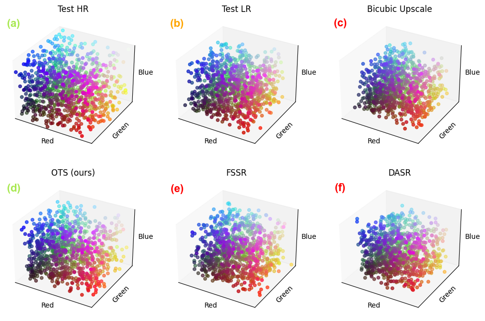
Dataset	Test HR	Test LR	Bicubic	OTS (ours)	FSSR	DASR
Variance	0.24 $\pm 0.01$	0.17 $\pm 0.01$	0.15 $\pm 0.02$	0.20 $\pm 0.03$	0.17 $\pm 0.02$	0.15 $\pm 0.02$

Figure 7: Color palettes and their variance for Test HR, LR datasets and solutions of Bicubic Upscale, OTS, FSSR, DASR methods on AIM19.

We additionally demonstrate the bias issue by comparing color palettes of HR images and super-resolution results of different methods, see Figure 7. We construct palettes by choosing random image pixels from dataset images and representing them as an RGB point cloud in $[0,1]^{3}\subset\mathbb{R}^{3}$. Figure 7 shows that OTS (d) captures large contrast of HR (a) images (variance of its palette), while FSSR (e), DASR (f), Bicubic Upscale (c) palettes are less contrastive and closer to LR (b). We construct palettes 100 times to evaluate their average contrast (variance). The metric quantitatively confirms that our OTS method better captures the contrast of HR dataset, while GAN-based methods (FSSR and DASR) are notably biased towards LR dataset statistics (low contrast).

Appendix C Training Details

Perceptual cost. In 7.2 we test following perceptual cost as $b$:

$$b(x^{\text{up}},y)=\text{MSE}(x^{\text{up}},y)+\nicefrac{{1}}{{3}}\cdot\text{MAE}(x^{\text{up}},y)+\nicefrac{{1}}{{50}}\cdot\sum_{k\in\{3,8,15,22\}}\text{MSE}\big{(}f_{k}(x^{\text{up}}),f_{k}(y)\big{)},$$

where $f_{k}$ denotes the features of the $k$th layer of a pre-trained VGG-16 network (Simonyan & Zisserman, 2014), MAE is the mean absolute error $\text{MAE}(x,y)=\frac{\|x-y\|_{1}}{\dim(\mathcal{Y})}$.

Dynamic transport cost. In the preliminary experiments, we used bicubic upsampling as the “Up" operation. Later, we found that the method works better if we gradually change the upsampling. We start from the bicubic upsampling. Every $k_{c}$ iterations of $f_{\omega}$ (see Table 4), we change the cost to $c(x,y)=b\big{(}T_{\theta}^{\prime}(x),y\big{)}$, where $T_{\theta}^{\prime}$ is a fixed frozen copy of the currently learned SR map $T_{\theta}$.

Hyperparameters. For EDSR, we set the number of residual blocks to 64, the number of features to 128, and the residual scaling to 1. For UNet, we set the base factor to 64. The training details are given in Table 4. We provide a comparison of the hyperparameters of FSSR, DASR and OTS (ours) in Table 5. In contrast to FSSR and DASR, our method does not contain a degradation part. This helps to notably reduce the amount of tunable hyperparameters.

Optimizer. We employ Adam (Kingma & Ba, 2014).

Computational complexity. Training OTS with EDSR as the transport map and the perceptual transport cost on AIM 2019 dataset takes $\approx 4$ days on a single Tesla V100 GPU.

Experiment	$\text{dim}(\mathcal{X})$	$\text{dim}(\mathcal{Y})$	$f$	$T$	$k_{T}$	$lr_{f}$	$lr_{T}$	Initial cost	Total iters ($f$)	Cost update every	Batch size
Benchmark (7.1)	$3\times 64\times 64$	$3\times 64\times 64$	ResNet	UNet	10	$10^{-4}$	$10^{-4}$	MSE	10K	$-$	64
Celeba (D)	$3\times 16\times 16$	$3\times 64\times 64$		Bilinear + UNet	15			Bicubic + MSE	100K	25K	64
				EDSR	15				100K	25K	64
AIM-19 (7.2)	$3\times 32\times 32$ (patches)	$3\times 128\times 128$ (patches)		EDSR	15				50K	25K	8
				EDSR	10			Bicubic + VGG	50K	20K	8

Table 4: Hyperparameters that we use in the experiments with our Algorithm 1.

Method	Degradation part	Super-resolution part	Total
FSSR	2 neural networks; 2 optimizers; 2 schedulers; 1 adversarial loss; 1 content loss ($\ell_{1}$+perceptual)	2 neural networks; 2 optimizers; 2 schedulers; 1 adversarial loss; 1 content loss ($\ell_{1}$+perceptual)	4 neural networks; 4 optimizers; 4 schedulers; 2 adversarial losses; 2 content losses ($\ell_{1}$+perceptual)
DASR	2 neural networks; 2 optimizers; 2 schedulers; 1 adversarial loss; 1 content loss ($\ell_{1}$+perceptual)	2 neural networks; 2 optimizers; 2 schedulers; 1 adversarial loss; 1 content loss ($\ell_{1}$+perceptual)	4 neural networks; 4 optimizers; 4 schedulers; 2 adversarial losses; 2 content losses ($\ell_{1}$+perceptual)
OTS (ours)	$-$	2 neural networks; 2 optimizers; 1 cost ($\ell_{2}$+$\ell_{1}$+perceptual)	2 neural networks; 2 optimizers; 1 cost ($\ell_{2}$+$\ell_{1}$+perceptual)

Table 5: Comparison of hyperparameters used in FSSR, DASR and OTS (ours) methods.

Appendix D Image Super-Resolution of Faces

We conduct an experiment using CelebA (Liu et al., 2015) faces to test the applicability of OT for unpaired SR. We test our Algorithm 1 with MSE as the cost and UNet or EDSR as the transport map.

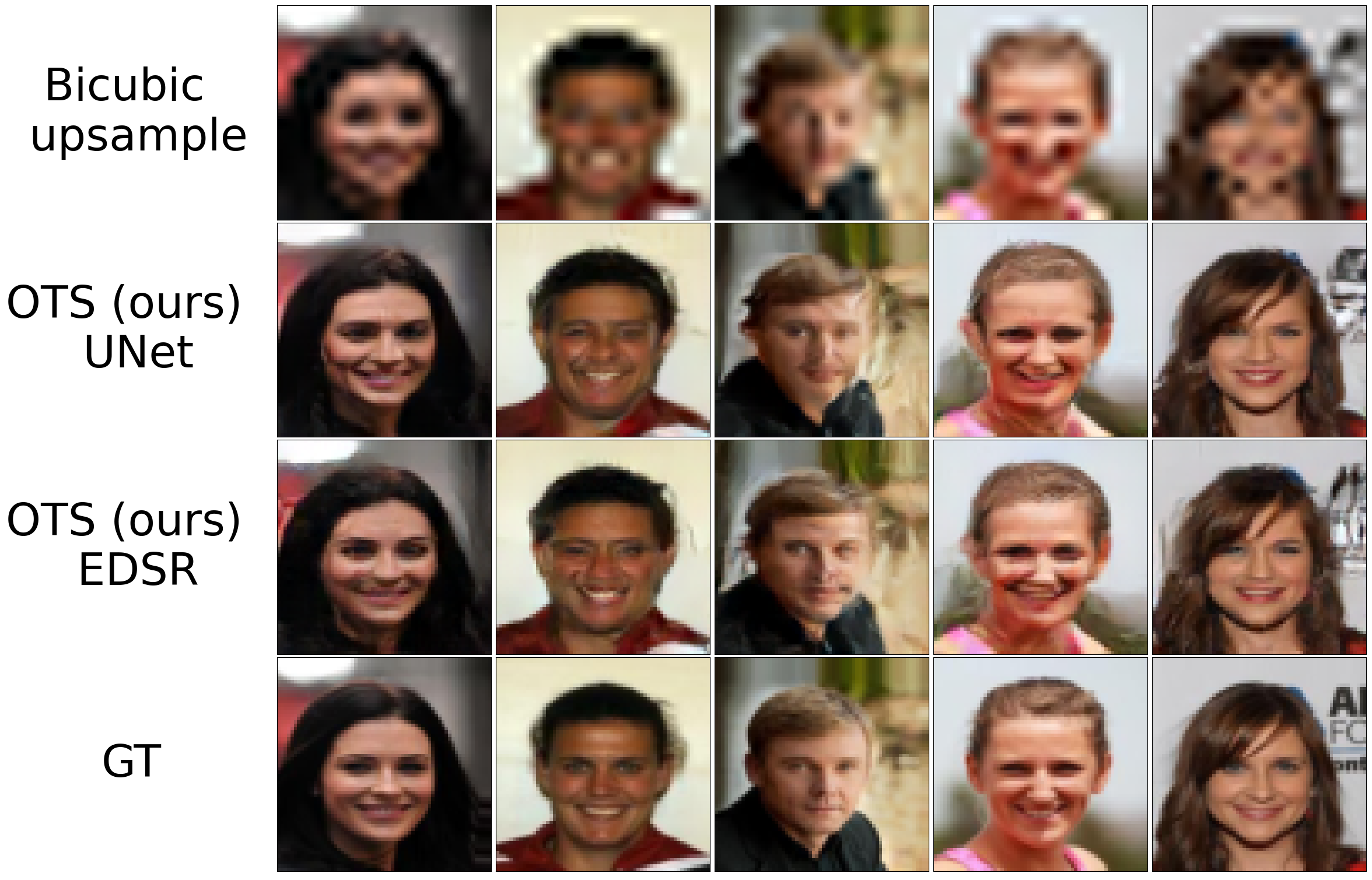
Figure 8: Qualitative results of OTS (ours) on CelebA.

Method	FID $\downarrow$	PSNR $\uparrow$	SSIM $\uparrow$	LPIPS $\downarrow$
Bicubic upsample	130.72	22.73	0.756	0.303
OTS (ours) UNet	12.32	22.10	0.740	0.058
OTS (ours) EDSR	15.87	22.33	0.747	0.054

Table 6: Comparison of OTS (ours) with the bicubic upsampling on CelebA dataset. The 1st and 2nd best results are highlighted in green and blue, respectively.

Pre-processing and train-test split. We resize images to $64\times 64$ px. We adopt the unpaired train-test split from (Rout et al., 2022, 5.2). We split the original HR dataset in 3 parts A, B, C containing 90K, 90K, 22K samples, respectively. We apply the bicubic downsample to each image and obtain the LR dataset ($16\!\times\!16$ faces). For training, we use LR part A, HR part B. For testing, we use parts C.

Metrics. We compute PSNR, SSIM, LPIPS and FID metrics on the test part, see Table 6.

Appendix E Additional Results on AIM19

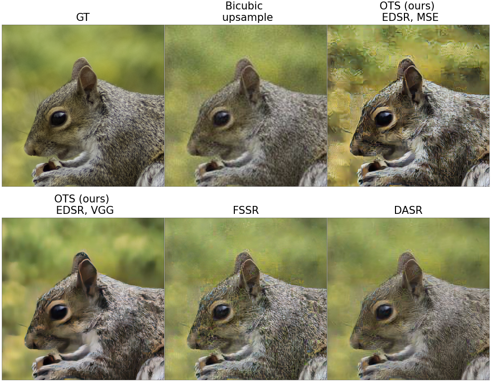
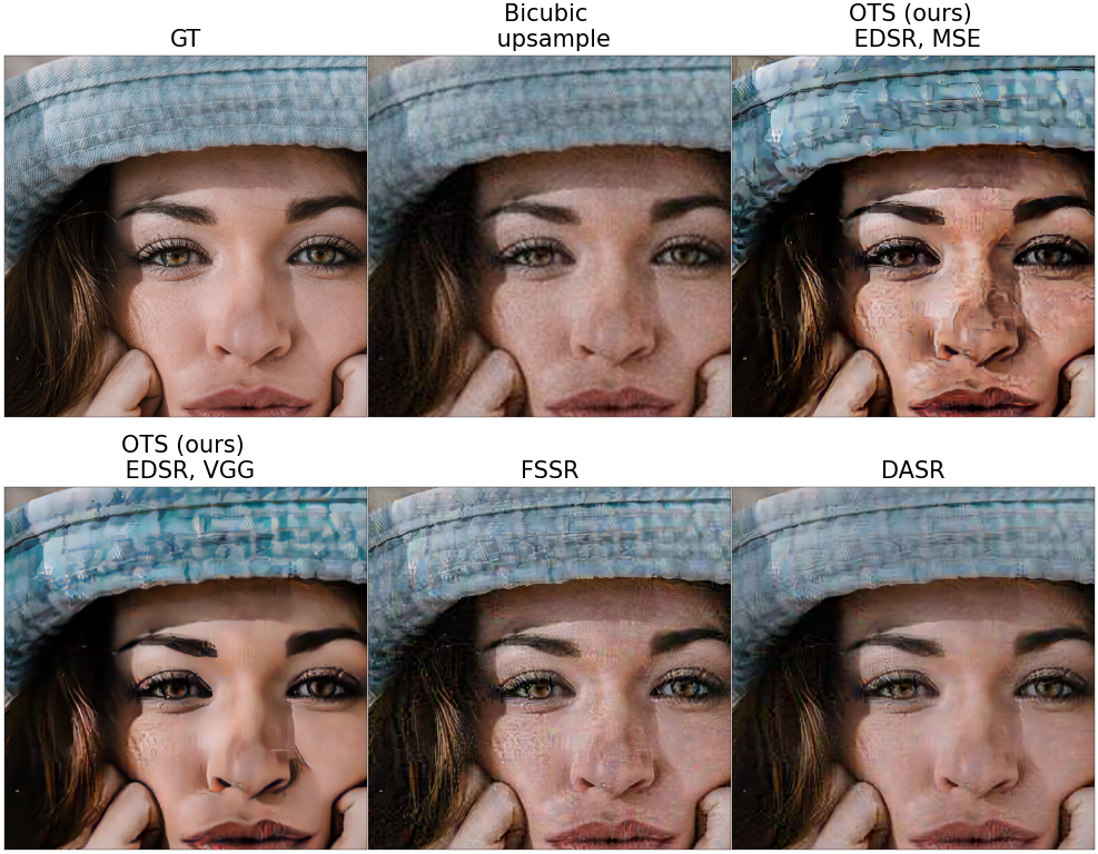
Figure 9: Additional qualitative results of OTS (ours), bicubic upsample, FSSR and DASR on AIM 2019 (800$\times$800 crops).

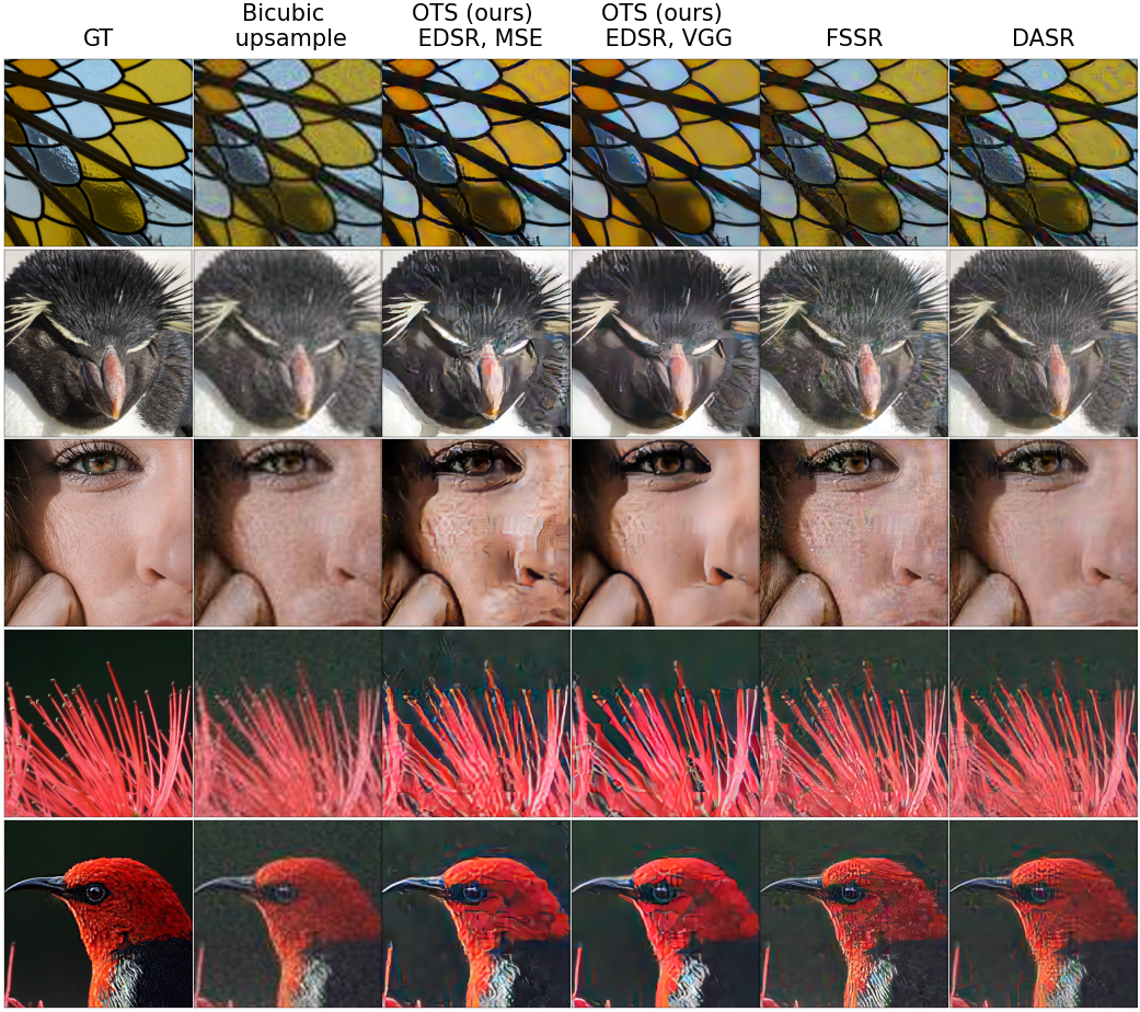
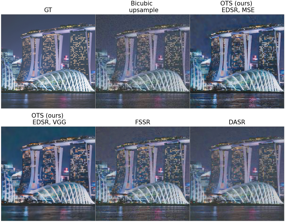
Figure 10: Additional qualitative results of OTS (ours), bicubic upsample, FSSR and DASR on AIM 2019. The sizes of crops on the 1st and 2nd images are 350$\times$350 and 800$\times$800, respectively.

References

- Arjovsky & Bottou (2017) Martin Arjovsky and Léon Bottou. Towards principled methods for training generative adversarial networks. arXiv preprint arXiv:1701.04862, 2017.
- Arjovsky et al. (2017) Martin Arjovsky, Soumith Chintala, and Léon Bottou. Wasserstein generative adversarial networks. In International conference on machine learning, pp. 214–223. PMLR, 2017.
- Balaji et al. (2020) Yogesh Balaji, Rama Chellappa, and Soheil Feizi. Robust optimal transport with applications in generative modeling and domain adaptation. Advances in Neural Information Processing Systems, 33:12934–12944, 2020.
- Bissoto et al. (2021) Alceu Bissoto, Eduardo Valle, and Sandra Avila. Gan-based data augmentation and anonymization for skin-lesion analysis: A critical review. In Proceedings of the IEEE/CVF Conference on Computer Vision and Pattern Recognition, pp. 1847–1856, 2021.
- Bousquet et al. (2017) Olivier Bousquet, Sylvain Gelly, Ilya Tolstikhin, Carl-Johann Simon-Gabriel, and Bernhard Schoelkopf. From optimal transport to generative modeling: the vegan cookbook. arXiv preprint arXiv:1705.07642, 2017.
- Bulat et al. (2018) Adrian Bulat, Jing Yang, and Georgios Tzimiropoulos. To learn image super-resolution, use a gan to learn how to do image degradation first. European Conference on Computer Vision, 09 2018.
- Fan et al. (2021) Jiaojiao Fan, Shu Liu, Shaojun Ma, Yongxin Chen, and Haomin Zhou. Scalable computation of monge maps with general costs. arXiv preprint arXiv:2106.03812, 2021.
- Fritsche et al. (2019) Manuel Fritsche, Shuhang Gu, and Radu Timofte. Frequency separation for real-world super-resolution. In IEEE/CVF International Conference on Computer Vision (ICCV) Workshops, 2019.
- Goodfellow et al. (2014) Ian Goodfellow, Jean Pouget-Abadie, Mehdi Mirza, Bing Xu, David Warde-Farley, Sherjil Ozair, Aaron Courville, and Yoshua Bengio. Generative adversarial nets. In Advances in neural information processing systems, pp. 2672–2680, 2014.
- Gulrajani et al. (2017) Ishaan Gulrajani, Faruk Ahmed, Martin Arjovsky, Vincent Dumoulin, and Aaron C Courville. Improved training of Wasserstein GANs. In Advances in Neural Information Processing Systems, pp. 5767–5777, 2017.
- He et al. (2016) Kaiming He, Xiangyu Zhang, Shaoqing Ren, and Jian Sun. Deep residual learning for image recognition. In Proceedings of the IEEE conference on computer vision and pattern recognition, pp. 770–778, 2016.
- Heusel et al. (2017) Martin Heusel, Hubert Ramsauer, Thomas Unterthiner, Bernhard Nessler, and Sepp Hochreiter. GANs trained by a two time-scale update rule converge to a local nash equilibrium. In Advances in neural information processing systems, pp. 6626–6637, 2017.
- Ji et al. (2020) Xiaozhong Ji, Yun Cao, Ying Tai, Chengjie Wang, Jilin Li, and Feiyue Huang. Real-world super-resolution via kernel estimation and noise injection. In 2020 IEEE/CVF Conference on Computer Vision and Pattern Recognition Workshops (CVPRW), pp. 1914–1923, 2020.
- Kantorovitch (1958) Leonid Kantorovitch. On the translocation of masses. Management Science, 5(1):1–4, 1958.
- Kim et al. (2020) Gwantae Kim, Jaihyun Park, Kanghyu Lee, Junyeop Lee, Jeongki Min, Bokyeung Lee, David K. Han, and Hanseok Ko. Unsupervised real-world super resolution with cycle generative adversarial network and domain discriminator. In Proceedings of the IEEE/CVF Conference on Computer Vision and Pattern Recognition Workshops (CVPRW), pp. 1862–1871, June 2020.
- Kingma & Ba (2014) Diederik P Kingma and Jimmy Ba. Adam: A method for stochastic optimization. arXiv preprint arXiv:1412.6980, 2014.
- Korotin et al. (2021) Alexander Korotin, Lingxiao Li, Aude Genevay, Justin M Solomon, Alexander Filippov, and Evgeny Burnaev. Do neural optimal transport solvers work? a continuous wasserstein-2 benchmark. Advances in Neural Information Processing Systems, 34, 2021.
- Krizhevsky et al. (2012) Alex Krizhevsky, Ilya Sutskever, and Geoffrey E. Hinton. Imagenet classification with deep convolutional neural networks. In Proceedings of the 25th International Conference on Neural Information Processing Systems - Volume 1, NIPS’12, pp. 1097–1105, Red Hook, NY, USA, 2012. Curran Associates Inc.
- Lai et al. (2017) Wei-Sheng Lai, Jia-Bin Huang, Narendra Ahuja, and Ming-Hsuan Yang. Deep laplacian pyramid networks for fast and accurate super-resolution. In Proceedings of the IEEE conference on computer vision and pattern recognition, pp. 624–632, 2017.
- Ledig et al. (2017) Christian Ledig, Lucas Theis, Ferenc Huszár, Jose Caballero, Andrew Cunningham, Alejandro Acosta, Andrew Aitken, Alykhan Tejani, Johannes Totz, Zehan Wang, et al. Photo-realistic single image super-resolution using a generative adversarial network. In Proceedings of the IEEE conference on computer vision and pattern recognition, pp. 4681–4690, 2017.
- Li et al. (2017) Chun-Liang Li, Wei-Cheng Chang, Yu Cheng, Yiming Yang, and Barnabás Póczos. MMD GAN: Towards deeper understanding of moment matching network. In Advances in Neural Information Processing Systems, pp. 2203–2213, 2017.
- Lim et al. (2017) Bee Lim, Sanghyun Son, Heewon Kim, Seungjun Nah, and Kyoung Mu Lee. Enhanced deep residual networks for single image super-resolution. In Proceedings of the IEEE conference on computer vision and pattern recognition workshops, pp. 136–144, 2017.
- Liu et al. (2019) Huidong Liu, Xianfeng Gu, and Dimitris Samaras. Wasserstein GAN with quadratic transport cost. In Proceedings of the IEEE International Conference on Computer Vision, pp. 4832–4841, 2019.
- Liu et al. (2015) Ziwei Liu, Ping Luo, Xiaogang Wang, and Xiaoou Tang. Deep learning face attributes in the wild. In Proceedings of International Conference on Computer Vision (ICCV), December 2015.
- Lu et al. (2020) Guansong Lu, Zhiming Zhou, Jian Shen, Cheng Chen, Weinan Zhang, and Yong Yu. Large-scale optimal transport via adversarial training with cycle-consistency. arXiv preprint arXiv:2003.06635, 2020.
- Lugmayr et al. (2019a) Andreas Lugmayr, Martin Danelljan, and Radu Timofte. Unsupervised learning for real-world super-resolution. 2019 IEEE/CVF International Conference on Computer Vision Workshop (ICCVW), pp. 3408–3416, 2019a.
- Lugmayr et al. (2019b) Andreas Lugmayr, Martin Danelljan, Radu Timofte, Manuel Fritsche, Shuhang Gu, Kuldeep Purohit, Praveen Kandula, Maitreya Suin, AN Rajagoapalan, Nam Hyung Joon, et al. Aim 2019 challenge on real-world image super-resolution: Methods and results. In 2019 IEEE/CVF International Conference on Computer Vision Workshop (ICCVW), pp. 3575–3583. IEEE, 2019b.
- Maeda (2020) Shunta Maeda. Unpaired image super-resolution using pseudo-supervision. In Proceedings of the IEEE/CVF Conference on Computer Vision and Pattern Recognition, pp. 291–300, 2020.
- Mallasto et al. (2019) Anton Mallasto, Jes Frellsen, Wouter Boomsma, and Aasa Feragen. (q, p)-Wasserstein GANs: Comparing ground metrics for Wasserstein GANs. arXiv preprint arXiv:1902.03642, 2019.
- Mroueh et al. (2017) Youssef Mroueh, Chun-Liang Li, Tom Sercu, Anant Raj, and Yu Cheng. Sobolev gan. arXiv preprint arXiv:1711.04894, 2017.
- Nilsson & Akenine-Möller (2020) Jim Nilsson and Tomas Akenine-Möller. Understanding ssim. arXiv preprint arXiv:2006.13846, 2020.
- Nowozin et al. (2016) Sebastian Nowozin, Botond Cseke, and Ryota Tomioka. f-GAN: Training generative neural samplers using variational divergence minimization. In Advances in neural information processing systems, pp. 271–279, 2016.
- Rockafellar (1976) R Tyrrell Rockafellar. Integral functionals, normal integrands and measurable selections. In Nonlinear operators and the calculus of variations, pp. 157–207. Springer, 1976.
- Ronneberger et al. (2015) Olaf Ronneberger, Philipp Fischer, and Thomas Brox. U-net: Convolutional networks for biomedical image segmentation. In International Conference on Medical image computing and computer-assisted intervention, pp. 234–241. Springer, 2015.
- Rout et al. (2022) Litu Rout, Alexander Korotin, and Evgeny Burnaev. Generative modeling with optimal transport maps. In International Conference on Learning Representations, 2022. URL https://openreview.net/forum?id=5JdLZg346Lw.
- Santambrogio (2015) Filippo Santambrogio. Optimal transport for applied mathematicians. Birkäuser, NY, 55(58-63):94, 2015.
- Sejdinovic et al. (2013) Dino Sejdinovic, Bharath Sriperumbudur, Arthur Gretton, and Kenji Fukumizu. Equivalence of distance-based and rkhs-based statistics in hypothesis testing. The annals of statistics, pp. 2263–2291, 2013.
- Simonyan & Zisserman (2014) Karen Simonyan and Andrew Zisserman. Very deep convolutional networks for large-scale image recognition. arXiv preprint arXiv:1409.1556, 2014.
- Taigman et al. (2016) Yaniv Taigman, Adam Polyak, and Lior Wolf. Unsupervised cross-domain image generation. arXiv preprint arXiv:1611.02200, 2016.
- Villani (2003) Cédric Villani. Topics in optimal transportation. Number 58. American Mathematical Soc., 2003.
- Villani (2008) Cédric Villani. Optimal transport: old and new, volume 338. Springer Science & Business Media, 2008.
- Wang et al. (2021) Wei Wang, Haochen Zhang, Zehuan Yuan, and Changhu Wang. Unsupervised real-world super-resolution: A domain adaptation perspective. In Proceedings of the IEEE/CVF International Conference on Computer Vision, pp. 4318–4327, 2021.
- Wei et al. (2021) Yunxuan Wei, Shuhang Gu, Yawei Li, Radu Timofte, Longcun Jin, and Hengjie Song. Unsupervised real-world image super resolution via domain-distance aware training. In Proceedings of the IEEE/CVF Conference on Computer Vision and Pattern Recognition (CVPR), pp. 13385–13394, June 2021.
- Xie et al. (2019) Yujia Xie, Minshuo Chen, Haoming Jiang, Tuo Zhao, and Hongyuan Zha. On scalable and efficient computation of large scale optimal transport. volume 97 of Proceedings of Machine Learning Research, pp. 6882–6892, Long Beach, California, USA, 09–15 Jun 2019. PMLR. URL http://proceedings.mlr.press/v97/xie19a.html.
- Yuan et al. (2018) Yuan Yuan, Siyuan Liu, Jiawei Zhang, Yong bing Zhang, Chao Dong, and Liang Lin. Unsupervised image super-resolution using cycle-in-cycle generative adversarial networks. 2018 IEEE/CVF Conference on Computer Vision and Pattern Recognition Workshops (CVPRW), pp. 814–81409, 2018.
- Zhang et al. (2018a) Richard Zhang, Phillip Isola, Alexei A Efros, Eli Shechtman, and Oliver Wang. The unreasonable effectiveness of deep features as a perceptual metric. In CVPR, 2018a.
- Zhang et al. (2018b) Yulun Zhang, Kunpeng Li, Kai Li, Lichen Wang, Bineng Zhong, and Yun Fu. Image super-resolution using very deep residual channel attention networks. In ECCV, 2018b.
- Zhu et al. (2017) Jun-Yan Zhu, Taesung Park, Phillip Isola, and Alexei A Efros. Unpaired image-to-image translation using cycle-consistent adversarial networks. In Proceedings of the IEEE international conference on computer vision, pp. 2223–2232, 2017.