The interplay between compact and molecular structures
in tetraquarks

Abstract

Due to the cluster reducibility of multiquark operators, a strong interplay exists in tetraquarks between the compact structure, resulting from the direct confining forces acting on quarks and gluons, and the molecular structure, dominated by the mesonic clusters. This issue is studied within an effective field theory approach, where the compact tetraquark is treated as an elementary particle. The key ingredient of the analysis is provided by the primary coupling constant of the compact tetraquark to the two mesonic clusters. Under the influence of this coupling, an initially formed compact tetraquark bound state evolves towards a new structure, where a molecular configuration is also present. In the strong-coupling limit, the evolution may end with a shallow bound state of the molecular type. The strong-coupling regime is also favored by the large-$N_{c}$ properties of QCD. The interplay between compact and molecular structures may provide a natural explanation of the existence of many shallow bound states.

I Introduction and summary

The experimental discoveries, during the last two decades, of many new particle candidates, corresponding to “exotic hadrons” [1, 2, 3, 4, 5, 6, 7, 8, 9, 10, 11, 12], not fulfilling the scheme of the standard quark model [13, 14, 15, 16], has given rise to thorough theoretical investigations for the understanding of the nature and structure of these states; recent review articles can be found in [17, 18, 19, 20, 21, 22, 23, 24, 25, 26, 27, 28, 29].

The theoretical issue faced by exotic hadrons, also called “multiquark states”, is whether they are formed, like ordinary hadrons, by means of the confining forces that act on the quarks and gluons, or whether they are formed, like molecular states, by means of the effective forces that act on ordinary hadrons [16]. (The term “molecule” refers here to the color-neutral character of hadrons, in analogy with the molecules formed by atoms [30, 31].) In the former case, multiquark states are expected to be compact objects, while in the latter case, they are expected to be loosely bound states. For the formation of compact multiquark states, the diquark model, in which two quarks form a preliminary tight system, provides the simplest mechanism to reach that goal [32, 33, 34, 35]. Molecular-type states [36, 30, 31, 37], also called “hadronic molecules”, are studied by means of effective field theories, based on approximate symmetry properties and nonrelativistic approximation [38, 39, 40, 41, 42, 43, 44, 45].

The reason these two competing alternatives are arising is related to the fact that the multiquark operators that generate multiquark states are not color-irreducible, in contrast to the ordinary hadron case, in the sense that they are decomposable along combinations of clusters of ordinary hadron operators [16, 46]. There are, therefore, two different ways of considering the construction of a multiquark state, as depicted above. The main issue is which one reproduces the most faithful description of reality. The existence or emergence of hadronic clusters inside a multiquark state might be an indication of a kind of instability when the state is built out of confining forces. It might, at some stage, dislocate into the clusters, or, in the case of a bound state, evolve towards another state, dominated by the clusters, that is, towards a molecular-type state.

A theoretical hint to analyze the problem is provided by the study of the energy balance of the two types of configuration [29]. This is most easily done for heavy or static quarks, for which lattice calculations are available [47, 48, 49, 50, 51, 52, 53]. In the strong coupling limit of lattice theory, analytic expressions are obtained by means of Wilson-loop expectation values, which satisfy the area law, or, more generally, are saturated by minimal surfaces; the corresponding predictions have been verified by direct numerical calculations on the lattice (cf. previous references). The qualitative result that emerges from the latter calculations is the following. When the quarks and antiquarks of the multiquark state are gathered into a small volume, it is the compact multiquark configuration that is energetically favored, while in situations where the quarks and antiquarks are seperated from each other at larger distances, it is the cluster-type configurations that are energetically favored. Therefore, there are nonzero probabilities for each type of configuration to occur for the description of the multiquark state. However, since quarks and antiquarks are moving objects and generally reaching, even with small probabilities, large distances, whose integrated volume may be much larger than the small volume of the compact configuration, one expects that an initially formed compact state would gradually evolve towards a cluster-type configuration, typical of a molecular state. In coordinate space, the core of the multiquark state would be better described by the compact representation, whereas the outer layer would be better described by the molecular representation. The relative weight of each representation would, of course, depend on specific parameters, such as the quark masses and the quantum numbers that are involved. The above results have led, in spectroscopic calculations, to the introduction of the concept of “configuration-space-partitioning” (or for short “geometric partitioning”) which is realized in the so-called “flip-flop” potential model [55, 56, 57, 58, 59, 60, 61, 62, 63, 64, 65, 66, 67], which takes into account more faithfully the role played by each configuration in the formation of multiquark states. However, because of the complicated nature of the constraints, which are coordinate dependent, this model, apart from simplified cases, has not yet led to full spectroscopic results, to be compared, on quantitative grounds, with experimental data.

In principle, if the tetraquark bound state problem could have been solved with high precision, taking into account all interactions that act between quarks and gluons, one would obtain the exact knowledge about its structure. Unfortunately, this is not currently the case; one is obliged to adopt approximations and proceed step by step by including additional inputs to improve the predictions. As mentioned above, the simplest approximations are either the compact scheme or the molecular scheme. While the latter scheme, based on hadron-hadron interactions, has a sufficiently developed theoretical background, the former one needs further analysis. In the diquark model, the diquark being considered in particular in its color-antisymmetric representation (ignoring here spin degrees of freedom) within a very small volume (pointlike or almost pointlike approximation), one always has tetraquark (or multiquark) bound states [68, 69, 70, 71, 72, 73, 74]; this is due to the fact that, in that approximation, all forces acting on the various small volumes (or points) are of the attractive confining types. This is not the case of the molecular scheme, where the occurrence of a bound state depends on the strength of the attractive forces. Therefore, in the compact scheme, one is entitled to start with a tetraquark (or multiquark) candidate, with all its accompanying multiplicities. The main problem that is encountered here is the evaluation of the effect the mesonic (or hadronic) clusters could have on that bound state. The key ingredient which enters in the description of that effect is the effective coupling constant of the compact tetraquark to the meson clusters. One easily guesses that stronger the latter quantity is, more important is the transformation of the compact state into a cluster-like state, which ultimately might take the appearance of a molecular-type state.

It is the main objective of the present paper to evaluate the interplay between the compact and molecular structures of possibly existing tetraquark states. For this, we shall adopt methods of effective field theories, remaining at the same time at the level of simple qualitative features.

In effective field theories of mesons, interactions are described by meson exchanges and by contacts. At lower energies, the exchanged meson fields can be integrated out and one remains only with a theory with contact-type interactions [75, 76], which we call here the “lower-energy” theory. The correspondence between the parameters of the two types of theory is not, however, simple and a physical understanding of the results necessitates a more detailed investigation. We devote Sec. II to a presentation of this aspect of the problem. Taking into account the various physical conditions and known results, we propose, in Sec. III, an empirical formula, which relates, in an explicit way, the coupling constant of the lower-energy theory to that of the Yukawa-type theory, and allows an easy understanding of the conditions in which a bound state may emerge. In order to emphasize the qualitative features of the approach, we neglect spin effects and limit ourselves to scalar interactions with scalar particles, ultimately considered in the nonrelativistic limit. The resulting effective theory is then used to study the meson-meson interaction through the scattering amplitude and the determination of the possibly existing bound state properties. The corresponding scattering length and effective range are evaluated in Sec. IV. Some of the results of Secs. III and IV are well known in the literature and are presented here for the purpose of introducing the method of approach that is applied for more general cases.

The case of compact tetraquarks is studied in Sec. V. With respect to the meson clusters, the compact tetraquark can be represented, in first approximation, as an elementary particle, whose internal structure would be relevant only at short-distance scales. It is then essentially characterized by its mass and quantum numbers and described by means of its propagator. The tetraquark, because of its internal structure, has necessarily interactions with meson pairs, and in particular with those lying closest to its mass. In the simplest case of one meson-pair, one may introduce a bare coupling constant for the interaction tetraquark-two-mesons and analyze its influence on the properties of the tetraquark through the radiative corrections it induces. For the bound state case, it is assumed that the bare compact tetraquark mass lies below the two-meson threshold. It turns out that, in general, the compact-tetraquark–two-meson interaction shifts the binding energy of the tetraquark to lower values. In the strong coupling limit, the shift may even transform the compact tetraquark into a shallow bound state, typical of loosely bound hadronic molecules. This phenomenon is best represented by means of the “elementariness” parameter $Z$, introduced by Weinberg [36], which measures the probability of a bound state to be considered as elementary, the complementary quantity, $(1-Z)$, representing its “compositeness”. In the strong coupling limit, described above, $Z$ takes small values, approaching zero. In parallel, the physical coupling constant of the tetraquark to two mesons tends also to zero in the same limit. The value of $Z$ is also measured by means of the scattering length and the effective range parameter, the latter taking negative values when $Z\neq 0$.

These results, which are the main outcome of the present paper, provide a more refined understanding of the structure of observed tetraquark candidates. Many shallow bound states, which are typical of molecular states, might have a compact origin, provided $Z\neq 0$. They would be the result of the deformation, under the influence of the mesonic clusters, of the initially formed compact tetraquark. This is another illustration of the dual representation of the tetraquark found in lattice theory on the basis of the energy balance analysis [47, 48, 49, 50, 51, 52, 53].

On more general grounds, shallow bound states are usually considered as belonging to universality classes, whose binding energy values are not naturally explained by means of the interaction scales of the system [77]. The previous results bring a new lighting to that problem in the case of tetraquarks. The coupling constant compact-tetraquark–meson-clusters introduces an additional scale parameter, whose strong-coupling limit naturally explains the origin of the shallowness.

The case of resonances occurs when the bare mass of the compact tetraquark lies above the two-meson threshold. Here, however, contrary to the bound state case, additional constraints appear for the existence of a physical resonance. The latter may exist only in the weak-coupling regime. Large values of the coupling constant resend the state to the bound state domain, while for a finite interval of the coupling constant, occurring prior to the strong-coupling regime, the tetraquark state may disappear from the spectrum.

Section VI brings complementary informations with respect to Sec. V, by also considering, in addition to the tetraquark-two-meson interaction effect, the influence of meson-meson interactions, which now renormalize the primary (bare) coupling constant and introduce a competing effect coming from direct molecular-type forces. The qualitative conclusions drawn in Sec. V remain, however, valid. Section VII is devoted to an analysis of the problem in the large-$N_{c}$ limit of QCD. In that limit, the theory provides additional support to the dominance of the strong-coupling regime in the effective interaction compact-tetraquark–meson-clusters. Conclusion follows in Sec. VIII. A few detailed analytic expressions, approximating energy eigenvalues, are gathered in the Appendix.

II Reduction to contact-type interactions

Effective field theories, which result from the integration of fields operating mainly at high energies, are generally characterized by the presence of contact-type interactions. Often, depending on the energy scale that is considered, these coexist with ordinary-type interactions, whose prototype is the Yukawa interaction, responsible of meson exchanges between interacting particles. At lower energies, the exchange-meson fields themselves are integrated out and one remains only with contact-type interactions. A representative example of such a theory is chiral perturbation theory [38, 39, 40], in which the interacting particles are the pseudo-Goldstone bosons and where all other massive particle fields have been integrated out. However, explorations of more refined properties, related to spectroscopic problems and to the physical interpretation of numerical values of parameters, may require a more detailed knowledge of the connection between the lower-energy theory and its higher-energy generator.

II.1 Spectroscopic properties of the higher-energy theory

To illustrate the above aspect of the question, we shall consider, following Reference [76], a higher-energy theory, where two massive scalar particles, with masses $m_{1}$ and $m_{2}$, interact by means of the exchange of a scalar particle with mass $\mu$, described by the interaction Lagrangian density

$$\mathcal{L}_{I}=\sum_{i=1}^{2}2m_{i}g\phi_{i}^{\dagger}\phi_{i}\varphi,$$ (1)

where, for simplicity, after factorizing, for dimensionality reasons, the mass terms $2m_{i}$, we have chosen the same (dimensionless) coupling constant $g$ for the two particles. The fields $\phi_{i}$ ($i=1,2$) correspond to those of the external massive particles, while $\varphi$ corresponds to the exchanged particle field.

The scattering amplitude of the process $\{1(p_{1}^{\prime})+2(p_{2}^{\prime})\rightarrow 1(p_{1})+2(p_{2})\}$ is given, in lowest order in $g$, by the Born term, or the ladder diagram:

$$i\mathcal{T}=-i\frac{4m_{1}m_{2}g^{2}}{q^{2}-\mu^{2}+i\epsilon},$$ (2)

where $q$ is the momentum transfer: $q=p_{1}-p_{1}^{\prime}=p_{2}^{\prime}-p_{2}$. This term iteratively generates higher-order diagrams, representing the series of ladder-type diagrams, which plays a basic role in a possible production of bound states. They are represented in Fig. 1.

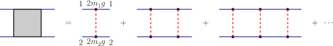
Figure 1: The meson-meson scattering amplitude in terms of the series of ladder diagrams.

A complete study of the theory requires the evaluation of the effects of self-energy and vertex corrections. These, however, do not play a fundamental role in the extraction of the main qualitative features that are of interest for our purpose and will be ignored.

The bound state problem in the nonrelativistic limit can be studied by means of the Schrödinger equation. The latter is obtained from the Bethe–Salpeter equation, with the kernel considered in the ladder approximation, represented by the right-hand side of Eq. (2). One has first to use the instantaneous approximation, where one neglects, in the cm frame, the temporal component of the momentum transfer $q$, and then to take the nonrelativistic limit. The Schrödinger equation in $x$-space is:

$$E\psi(\mathbf{x})=\Big{(}\frac{\mathbf{p}^{2}}{2m_{r}}+V(r)\Big{)}\psi(\mathbf{x}),\ \ \ r=\sqrt{\mathbf{x}^{2}},\ \ \ \mathbf{x}=\mathbf{x}_{1}-\mathbf{x}_{2},\ \ \ m_{r}=\frac{m_{1}m_{2}}{(m_{1}+m_{2})},$$ (3)

where $V(r)$ is the well-known Yukawa potential:

$$V(r)=-(\frac{g^{2}}{4\pi})\frac{1}{r}e^{{\displaystyle-\mu r}}.$$ (4)

Making in (3) the changes of variable and parameter [78]

$$\mathbf{x}=\mathbf{x}^{\prime}/\mu,\ \ \ \ \mathbf{p}=\mu\mathbf{p^{\prime}},\ \ \ \ E=\frac{\mu^{2}}{2m_{r}}E^{\prime},\ \ \ \ g^{2}=\overline{g}^{2}\frac{\mu}{2m_{r}},$$ (5)

one reduces the Schrödinger equation to a dimensionless equation with a single parameter, $\overline{g}^{2}$:

$$E^{\prime}\psi(\mathbf{x}^{\prime})=\Big{(}\mathbf{p}^{\prime 2}-(\frac{\overline{g}^{2}}{4\pi})\frac{1}{r^{\prime}}e^{{\displaystyle-r^{\prime}}}\Big{)}\psi(\mathbf{x}^{\prime}).$$ (6)

Compared to the Coulomb potential, the Yukawa potential (4) is of the short-range type and hence not all values of $\overline{g}^{2}$ may produce bound states. There exists a critical value of it, $\overline{g}_{\mathrm{cr}}^{2}=1.68\times(4\pi)$ [76, 78], below which bound states do not exist. Their existence is ensured by the inequality

$$(\frac{\overline{g}^{2}}{4\pi})\geq(\frac{\overline{g}_{\mathrm{cr}}^{2}}{4\pi})=1.68.$$ (7)

At the critical value of the coupling constant, a zero-energy bound state appears. When $\overline{g}^{2}$ increases, gradually new bound states appear, while the ground state binding energy itself increases.

In more general cases, one may have the sum of several Yukawa potentials with different meson exchanges. In such cases, one loses the notion of a universal coupling constant squared $\overline{g}^{2}$. To continue exploring qualitative aspects of the problem, it would be advantageous to approximate the sum by a single Yukawa potential with a mean exchanged mass and a mean coupling constant.

General qualitative properties of the Yukawa potential, concerning the related spectroscopy and the poles of the corresponding $S$-matrix, could be obtained by considering the soluble model of the spherically symmectric rectangular potential well, which is a prototype of short-range potentials [79, 80]. If $V_{0}$ is the depth of the potential and $R$ its width, then there is a correspondence between $\overline{g}^{2}/(4\pi)$ and the product $2m_{r}V_{0}R^{2}\equiv A^{2}$. The critical value of $A^{2}$ is equal to $\pi^{2}/4=2.46$, which is of the same order of magnitude as $\overline{g}_{\mathrm{cr}}^{2}/(4\pi)$ [Eq. (7)].

II.2 The lower-energy effective field theory

A lower-energy effective field theory can be obtained by integrating out the mediator field $\varphi$. One then obtains a theory where the only remaining fields are the $\phi_{i}$s. Their interactions are represented by an infinite series of contact terms with increasing powers of products of $\phi_{i}$s, also possibly containing derivative couplings. They are classified according to their dimensionality and a systematic expansion is organized according to definite power counting rules. The coupling constants of the lower-energy theory are usually determined from matching conditions of the scattering amplitudes calculated in the two theories. At low energies, it is the lowest-dimension operator that is expected to provide the leading contribution. We stick in the following to that term. The corresponding Lagrangian density, for the mutual interaction of particles 1 and 2, is

$$\mathcal{L}_{I,\mathrm{eff}}=h\phi_{1}^{\dagger}\phi_{1}\phi_{2}^{\dagger}\phi_{2},$$ (8)

where $h$ is the coupling constant. This term, like (1), generates by iteration a chain of loop or bubble diagrams, which are represented in Fig. 2.

Figure 2: The meson-meson scattering amplitude in terms of the chain of loop diagrams generated by the contact term (8).

The problem that interests us is to what extent the lower-energy theory in its leading-order approximation, represented by the Lagrangian density (8), provides a faithful description of the higher-energy theory, considered in the ladder-approximation, in the bound state domain.

Similar searches as above have been undertaken long ago in the past, although with a different viewpoint. In this respect, Reference [81], provides a rather detailed account of the corresponding approach. The objective has been to establish an equivalence theorem between the two theories described by Lagrangian densities of the types of (1) and (8), respectively, the external particles being here fermions. Putting aside the question of the nonrenormalizability of the four-Fermi interaction theory, the approach has consisted in considering the first ladder diagram of Fig. 1, together with the radiative corrections of the exchanged meson propagator, and searching for conditions of equivalence of the chain of diagrams of Fig. 2, considered in the $t$-channel. Our line of investigation is rather different, being based on the effective field theory approach, searching for matching conditions for the leading terms of the scattering amplitude in the $s$-channel.

Coming back to the present approach with its matching conditions, it turns out that all diagrams of Fig. 1, besides contributing to the coupling constants of higher-dimensional operators, also give contributions to the coupling constant $h$ of (8). Therefore, $h$, considered as a function of $g^{2}$ (or $\overline{g}^{2}$), has an expression in the form of an infinite series of it:

$$h=\sum_{n=0}^{\infty}h^{(n)},\ \ \ \ \ \ \ \ \ h^{(0)}=\frac{4m_{1}m_{2}}{\mu^{2}}g^{2},$$ (9)

where $h^{(n)}$ represents the contribution coming from the $n$-loop diagram (proportional to $(\frac{\overline{g}^{2}}{4\pi})^{n}h^{(0)}$). Notice that $h^{(0)}$ is positive. While the first few terms of the series of $h$ are explicitly calculable [76], the complete knowledge of the expression of $h$ in terms of $g^{2}$ is not known. It is evident, from the lower-bound (7), that, for the bound state problem, one cannot be satisfied by a perturbative expansion of $h$, but rather a full nonperturbative expression of it will be needed in order to understand and interpret the bound state properties of the lower-energy theory in terms of those of the higher-energy theory.

III Nonperturbative properties of the coupling constant of the low-energy theory

The nonperturbative properties of the coupling constant $h$ can be deduced from the study of the bound state problem of the low-energy theory. The result of the latter problem is well known in the literature [75, 76] and we briefly sketch the corresponding procedure. The scattering amplitude resulting from the chain of diagrams of Fig. 2 is a geometric series expressible in terms of the two-point loop integral $J(s)$:

$$\mathcal{T}\equiv\mathcal{T}_{\mathrm{eff}}=\frac{h}{1-ihJ(s)},\ \ \ \ \ \ s=P^{2}=(p_{1}+p_{2})^{2},$$ (10)

$$J(s)=\int\frac{d^{4}k}{(2\pi)^{4}}\frac{i}{(p_{1}+k)^{2}-m_{1}^{2}+i\epsilon}\frac{i}{(p_{2}-k)^{2}-m_{2}^{2}+i\epsilon}.$$ (11)

$J(s)$ is divergent, but its divergence can be absorbed in $h$ by renormalization. Defining $J^{\mathrm{r}}$ as the regularized (finite) part of $J$ and $J^{\mathrm{div}}$ as its diverging part, such that

$$J(s)=J^{\mathrm{div}}+J^{\mathrm{r}}(s),$$ (12)

one obtains

$$\frac{1}{h}-iJ^{\mathrm{div}}=\frac{1}{h^{\mathrm{r}}}\ \ \ \ \ \ \ \Longleftrightarrow\ \ \ \ \ \ \ \frac{h}{1-ihJ(s)}=\frac{h^{\mathrm{r}}}{1-ih^{\mathrm{r}}J^{\mathrm{r}}(s)},$$ (13)

where $h^{\mathrm{r}}$ is the renormalized finite part of $h$. Notice that this renormalization implies that the unrenormalized $h$ is a vanishing quantity:

$$h=\frac{h^{\mathrm{r}}}{1+ih^{\mathrm{r}}J^{\mathrm{div}}}.$$ (14)

In the limit where, for finite $h^{\mathrm{r}}$, $iJ^{\mathrm{div}}\rightarrow\infty$, one has $h\rightarrow 0$.

Regularizing $J$ by dimensional regularization and keeping in the diverging part only mass-independent terms, $J^{\mathrm{r}}$ takes the following form:

$$J^{\mathrm{r}}(s)=\frac{i}{16\pi^{2}}\,\Big{[}\,\ln\Big{(}\frac{m_{1}m_{2}}{4\pi\overline{\mu}^{2}}\Big{)}+\frac{(m_{1}^{2}-m_{2}^{2})}{2s}\ln\Big{(}\frac{m_{1}^{2}}{m_{2}^{2}}\Big{)}+Q(s)\,\Big{]}.$$ (15)

$\overline{\mu}$ is the mass scale introduced by the dimensional regularization, whose value can be chosen at will; $Q(s)$ is defined in the complex $s$-plane, cut on the real axis from $s=(m_{1}+m_{2})^{2}$ to $+\infty$ and from $s=(m_{1}-m_{2})^{2}$ to $-\infty$, and has the expression

$$Q(s)=\frac{\sqrt{\lambda(s)}}{s}\,\ln\Big{(}\frac{\sqrt{s-(m_{1}+m_{2})^{2}}+\sqrt{s-(m_{1}-m_{2})^{2}}}{\sqrt{s-(m_{1}+m_{2})^{2}}-\sqrt{s-(m_{1}-m_{2})^{2}}}\Big{)},$$ (16)

where

$$\lambda(s)\equiv\lambda(s,m_{1}^{2},m_{2}^{2})=\Big{(}s-(m_{1}+m_{2})^{2}\Big{)}\Big{(}s-(m_{1}-m_{2})^{2}\Big{)}.$$ (17)

(The square-roots are defined for complex $s$ as $\sqrt{s-m^{2}}=e^{i\alpha/2}\sqrt{|s-m^{2}|}$, where $\alpha$ is the angle made by $(s-m^{2})$ with the positive real axis starting from $m^{2}$.) On the real axis, $Q(s)$ takes the following forms:

$$Q(s)=\left\{\begin{array}[]{l}-\frac{\sqrt{\lambda(s)}}{s}\ln\Big{(}\frac{\sqrt{(m_{1}+m_{2})^{2}-s}+\sqrt{(m_{1}-m_{2})^{2}-s}}{\sqrt{(m_{1}+m_{2})^{2}-s}-\sqrt{(m_{1}-m_{2})^{2}-s}}\Big{)},\ \ \ \ s<(m_{1}-m_{2})^{2},\\ +\frac{\sqrt{-\lambda(s)}}{s}\Big{[}\pi-2\arctan\Big{(}\frac{\sqrt{(m_{1}+m_{2})2-s}}{\sqrt{s-(m_{1}^{2}-m_{2}^{2})}}\Big{)}\Big{]},\ \ \ \ (m_{1}-m_{2})^{2}<s<(m_{1}+m_{2})^{2},\\ +\frac{\sqrt{\lambda(s)}}{s}\Big{[}\ln\Big{(}\frac{\sqrt{s-(m_{1}-m_{2})^{2}}+\sqrt{s-(m_{1}+m_{2})^{2}}}{\sqrt{s-(m_{1}-m_{2})^{2}}-\sqrt{s-(m_{1}+m_{2})^{2}}}\Big{)}\mp i\pi\Big{]},\\ \hskip 113.81102ptRe(s)>(m_{1}+m_{2})^{2},\ \ \ \ Im(s)=\pm\epsilon,\ \ \epsilon>0.\end{array}\right.$$ (18)

(The square-roots in (18) are defined with positive values, their arguments representing moduli. $J^{\mathrm{r}}(s)$ is finite at $s=0$.) Physical quantities should be independent of $\overline{\mu}$. Since $\mathcal{T}_{\mathrm{eff}}$ is such a quantity, this implies that $h^{\mathrm{r}}$ itself should be $\overline{\mu}$ dependent and should cancel the $\overline{\mu}$-dependence of $J^{\mathrm{r}}$. The absorption of the term $\ln\Big{(}\frac{m_{1}m_{2}}{4\pi\overline{\mu}^{2}}\Big{)}$ into a redefined $1/h^{\mathrm{r}}$, which amounts to also absorbing the same quantity into $J^{\mathrm{div}}$, is the simplest way of ensuring this. We shall adopt henceforth that procedure. It is advantageous to define $h^{\mathrm{r}}$ as having a simple physical interpretation. A natural choice is the value of $\mathcal{T}_{\mathrm{eff}}$ at the two-particle threshold [75]. We shall continue using the same notation for the redefined $h^{\mathrm{r}}$ and $J^{\mathrm{r}}$; then the redefined $J^{\mathrm{r}}$ obtains the form

$$J^{\mathrm{r}}(s)=\frac{i}{16\pi^{2}}\Big{[}\,\Big{(}\frac{1}{s}-\frac{1}{(m_{1}+m_{2})^{2}}\Big{)}\frac{(m_{1}^{2}-m_{2}^{2})}{2}\ln\Big{(}\frac{m_{1}^{2}}{m_{2}^{2}}\Big{)}+Q(s)\,\Big{]}.$$ (19)

The scattering amplitude (10) then takes the form, according to (13),

$$\mathcal{T}=\frac{h^{\mathrm{r}}}{1-ih^{\mathrm{r}}J^{\mathrm{r}}(s)}.$$ (20)

Bound states of $\mathcal{T}$ will be identified as tetraquark states of the molecular type, whose parameters and ingredients will be labeled by the indices $tm$; they correspond to the solutions of the equation

$$\frac{1}{h^{\mathrm{r}}}-iJ^{\mathrm{r}}(s_{tm})=0.$$ (21)

(We shall often omit, for the simplicity of notation and when no ambiguity is present, the index $\mathrm{r}$ from $h^{\mathrm{r}}$ and $J^{\mathrm{r}}$.) We restrict ourselves to the case of possible nonrelativistic solutions, located near the two-particle threshold. We introduce the nonrelativistic energy $E_{tm}$ through the definition

$$\sqrt{s_{tm}}=(m_{1}+m_{2})+E_{tm},$$ (22)

and, to simplify notations, we shall use henceforth the reduced dimensionless energy variable $e$ and bound state energy $e_{tm}$, respectively:

$$e\equiv\frac{E}{2m_{r}},\ \ \ \ \ \ \ \ e_{tm}\equiv\frac{E_{tm}}{2m_{r}},$$ (23)

where $m_{r}$ is the reduced mass [Eq. (3)]. Retaining, in the second of Eqs. (18), the leading term in $\sqrt{-e_{tm}}$, which is contained in its first piece, one finds a unique possible solution:

$$\sqrt{-e_{tm}}=-\frac{16\pi}{\alpha h},\ \ \ \ \ \ \ \alpha\equiv\frac{4m_{r}}{(m_{1}+m_{2})}.$$ (24)

The existence of the solution is conditioned by a negative value of $h$. This means that $h$ must have changed sign with respect to the perturbative expression $h^{(0)}$ [Eq. (9)]. To ensure the nonrelativistic interpretation of the solution, one must have a large value of $|h|$, such that

$$16\pi/|h|\ll 1.$$ (25)

When $|h|\rightarrow\infty$, the bound state approaches the two-particle threshold. On the other hand, when $h\rightarrow 0$ with negative values, the binding energy increases and tends to $\infty$.

The stability of the solution (24) in the presence of higher-order terms in $\sqrt{-e_{tm}}$ can be studied by also considering in $J^{\mathrm{r}}(s)$ terms of order $(-e)$, which are contained in the second term of $Q(s)$ [Eq. (18)] and the remaining terms of $J^{\mathrm{r}}(s)$ [Eq. (17)]. Accepting condition (25), the resulting equation continues reproducing the solution (24), but yields also a second solution, which lies far from the two-particle threshold and does not have the required nonrelativistic limit. Solution (24) remains therefore the only stable nonrelativistic solution of Eq. (21).

The behavior of the bound state energy with respect to the variations and the order of magnitude of the coupling constant $h$ is unusual. Generally, if a coupling constant of a theory increases up to infinity, one expects to find instabilities or phase transitions, while here one finds a smooth behavior in the vicinity of the two-particle threshold. Similarly, vanishing values of the coupling constant should lead the theory towards its perturbative regime. This means that the coupling constant $h$ of the low-energy theory cannot be interpreted as an elementary or an ordinary coupling constant. To interpret correctly its role, one should try to connect it more explicitly to the original coupling constant $g$ of the higher-energy theory. In the latter theory, the lowest bound state approaches the two-particle threshold when $g$ approaches its critical value $g_{\mathrm{cr}}$ from above. Therefore, negative values of $h$ correspond to values of $g$ greater than $g_{\mathrm{cr}}$. Large and negative values of $h$ would correspond to the approach $g\rightarrow g_{\mathrm{cr}}$, at which value $h$ would have a singularity. Vanishing of $h$ with negative values would correspond to the increasing of $g$ up to infinity. When $g$ is lower than $g_{\mathrm{cr}}$, $h$ should change sign and the system would enter in a phase characterized by the absence of bound states. Finally, the vanishing of $h$ with positive values would correspond to the approach to the perturbative regime. A schematic representation of these correspondences is shown in Fig. 3 [29].

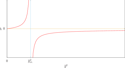
Figure 3: A schematic representation of the relationship between the low-energy coupling constant $h$ and the high-energy coupling constant $g$, the latter represented through $\overline{g}^{2}$ [Eq. (5)].

The exact relationship between $h$ and $g$ not being available at present, it would be useful to have an approximate or an empirical relation which qualitatively reproduces its main properties and allows for an easy understanding of the physical situation that is considered. For this, we propose the following formula between $h$ and $\overline{g}^{2}$ [Eq. (5)], the latter having a more universal meaning than $g^{2}$:

$$\frac{\alpha h}{16\pi}=\frac{2m_{r}}{\mu}\frac{\overline{g}^{2}}{4\pi}\frac{1}{(1-\overline{g}^{2}/\overline{g}_{\mathrm{cr}}^{2})(1+b\overline{g}^{2}/\overline{g}_{\mathrm{cr}}^{2})},\ \ \ \ \ \ b\simeq 0.5,$$ (26)

where $b$ is an empirical parameter, whose approximate value has been determined by numerical tests.

This formula is expected to be approximately valid in the nonrelativistic domain of the bound states. To test its validity, we have compared the bound state energies, calculated from the Schrödinger equation [(3)-(6)] and from the lower-energy theory [(24) and (26)], in units of $\mu^{2}/(2m_{r})$. The results are graphically represented in Fig. 4.

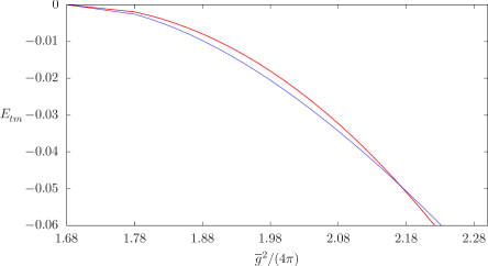
Figure 4: The bound-state energies calculated from the Yukawa potential (red line) and from the lower-energy theory (blue line), in units of $\mu^{2}/(2m_{r})$.

One finds a rather satisfactory matching of the two predictions. To have an idea of the values of the predicted binding energies, choosing $2m_{r}\simeq 2$ GeV (corresponding for instance to a system of $D\overline{D}$ or $D^{*}\overline{D}$ mesons) and $\mu\simeq 0.5-1.$ GeV (corresponding to the exchange of an effective scalar meson), one has for the unit of energy $\mu^{2}/(2m_{r})\simeq 25-100$ MeV; the value 0.06 of $-E_{tm}$ in Fig. 4 would correspond to a binding energy of $1.5-6$ MeV.

By expanding in (26) $\overline{g}^{2}$ around $\overline{g}_{\mathrm{cr}}^{2}$, one obtains from (24) the further approximation of $e_{tm}$ near the two-meson threshold:

$$e_{tm}\simeq-\Big{(}\frac{\mu}{2m_{r}}\Big{)}^{2}\Big{[}\Big{(}\frac{4\pi}{\overline{g}_{\mathrm{cr}}^{2}}\Big{)}(1+b)\Big{]}^{2}\Big{(}\frac{\overline{g}^{2}}{\overline{g}_{\mathrm{cr}}^{2}}-1\Big{)}^{2}.$$ (27)

The quadratic behavior of $e_{tm}$ with respect to the departure of $\overline{g}^{2}$ from $\overline{g}_{\mathrm{cr}}^{2}$ is typical of short-range potentials and can be verified on soluble models.

As a side remark, let us notice that the extension of the formula (26) to the relativistic domain necessitates more elaborate comparisons. The reason is that in the latter domain one has no longer a single energy unit and the corresponding generalization is not straightforward. Furthermore, in the higher-energy theory, the Bethe–Salpeter equation itself has difficulties to describe correctly the first relativistic corrections in the ladder approximation with covariant propagators [82]; one is obliged to use either the instantaneous approximation, or other quasipotential-type approaches, which reduce the Bethe–Salpeter equation to a three-dimensional equation. We shall be content, in the present work, to stick to the nonrelativistic domain, where many experimental data still require a detailed investigation.

One can also obtain, from the expression (20) of the scattering amplitude, the coupling constant of the bound state to the constituent mesons, appearing in the residue of the bound state pole. Designating by $M_{1}$ and $M_{2}$ the two constituent mesons, the scattering amplitude has the following behavior near the pole position of the bound state:

$$\mathcal{T}\simeq-\frac{(m_{1}+m_{2})^{2}g_{TM_{1}M_{2}}^{2}}{s-s_{tm}},$$ (28)

where $g_{TM_{1}M_{2}}$ represents the dimensionless coupling constant of the tetraquark to the two mesons, defined with the accompanying mass factor $(m_{1}+m_{2})$. Expanding in (20) $J^{\mathrm{r}}(s)$ around $s_{tm}$ and using (21), one obtains

$$(m_{1}+m_{2})^{2}g_{TM_{1}M_{2}}^{2}=\frac{1}{iJ^{\prime}(s_{tm})},$$ (29)

giving

$$g_{TM_{1}M_{2}}^{2}=32\pi\sqrt{-e_{tm}}.$$ (30)

One notices that the coupling constant decreases when the bound state approaches the two-particle threshold.

Let us finally emphasize, as is evident from the previous results and, in particular, from the structure of $\mathcal{T}$ [Eq. (10)], that the low-energy theory can reproduce, in the present scalar theory, only the ground state of the higher-energy theory.

IV Scattering length and effective range

The expression of the scattering amplitude (10) can also be used in the scattering domain, where only the $S$-wave contributes. Introducing the cm momentum $k=\sqrt{\lambda(s,m_{1}^{2},m_{2}^{2})}/(2\sqrt{s})$ [Eq. (17)] and expanding $J^{\mathrm{r}}(s)$ [(19) and the third of Eqs. (18)], considered above the cut, up to terms of order $k^{2}$, one finds

$$\mathcal{T}=\frac{8\pi(m_{1}+m_{2})}{\frac{8\pi(m_{1}+m_{2})}{h}+\frac{k^{2}}{\pi m_{r}}(1-d)-ik},$$ (31)

where we have defined

$$d=\frac{1}{2}\Big{(}\frac{m_{1}-m_{2}}{m_{1}+m_{2}}\Big{)}\ln(\frac{m_{1}}{m_{2}}).$$ (32)

On the other hand, $\mathcal{T}$ can be expressed in terms of the $S$-wave phase shift $\delta_{0}$ as

$$\mathcal{T}=\frac{8\pi\sqrt{s}}{k\cot\delta_{0}(k)-ik}.$$ (33)

The factor $\cot\delta_{0}(k)$ is itself expressed through a low-energy expansion in terms of the scattering length $a$ and the effective range $r_{e}$ [83]:

$$k\cot\delta_{0}(k)=-\frac{1}{a}+\frac{1}{2}r_{e}k^{2},$$ (34)

yielding the identifications

$$a=-\frac{h}{8\pi(m_{1}+m_{2})}=\frac{1}{2m_{r}\sqrt{-e_{tm}}},\ \ \ \ \ \ \ r_{e}=\frac{2}{\pi m_{r}}(1-d).$$ (35)

(The relativistic correction coming from the expansion of $\sqrt{s}$ in the numerator of $\mathcal{T}$, Eq. (33), has been neglected.) One finds that $a$ is proportional to $-h$ and, therefore, has the same type of behavior as $-h$ in terms of the coupling constant squared $\overline{g}^{2}$ (Fig. 3). (This has also been shown in [78].) According to whether $\overline{g}^{2}$ is greater or smaller than $\overline{g}_{\mathrm{cr}}^{2}$, $a$ is positive or negative. On the other hand, the parameter $d$ [Eq. (32)] is positive and in general, for physical applications, smaller than 1; the effective range $r_{e}$ is then predicted positive and small.

Of particular interest is the case of resonances, which appear as bumps in the cross section above the two-particle threshold. They correspond to complex poles of the scattering amplitude, lying below the cut of the real axis. To check the possible presence of complex poles, we go back to the expression (16) of $Q(s)$ in the complex plane, which can also be rewritten in the following form:

$$Q(s)=\frac{\sqrt{\lambda(s)}}{s}\,\Big{[}-i\pi+\ln\Big{(}\frac{\sqrt{s-(m_{1}-m_{2})^{2}}+\sqrt{s-(m_{1}+m_{2})^{2}}}{\sqrt{s-(m_{1}-m_{2})^{2}}-\sqrt{s-(m_{1}+m_{2})^{2}}}\Big{)}\Big{]}.$$ (36)

Using a definition of the type of (22), one has in approximate form, neglecting quadratic terms in $E$,

$$s-(m_{1}+m_{2})^{2}\simeq 2(m_{1}+m_{2})E,\ \ \ \ \ \ s-(m_{1}-m_{2})^{2}\simeq 4m_{1}m_{2}(1+\frac{E}{2m_{r}}).$$ (37)

The first equation shows that the complex variable $E$, considered as a vector, is parallel to $(s-(m_{1}+m_{2})^{2})$ in the $s$-plane and therefore one can transpose to $E$ the complex-plane analysis, with a right-hand cut starting at $E=0$. Making expansions in $\sqrt{e}$ and retaining terms up to order $e$, one obtains

$$Q(s)=\alpha\sqrt{e}\,(-i\pi+2\sqrt{e}).$$ (38)

($\alpha$ defined in Eq. (24).) $J(s)$ [Eq. (19)] then takes the form

$$J(s)=\frac{i}{16\pi^{2}}\alpha\sqrt{e}\,\Big{[}-i\pi+2\sqrt{e}(1-d)\Big{]},$$ (39)

where $d$ has been defined in (32). In the nonrelativistic domain, the second term is negligible in front of the first and the resonance equation takes the form

$$-i\sqrt{e_{R}}+\frac{16\pi}{\alpha h}=0,$$ (40)

which yields a purely imaginary solution for $\sqrt{e_{R}}$ and gives back the bound state solution (24). Formal resonance solutions can be obtained outside the nonrelativistic domain for small negative values of $h$ [$-\frac{\alpha h}{16\pi}<\frac{8}{\pi}(1-d)$], by including also the second term of the right-hand-side of (39); however, such values of $h$ correspond, according to the correspondence (26), to the strong-coupling limit of $\overline{g}^{2}$, which goes beyond the validity of the present nonrelativistic approximation.

The previous results mean that the present model does not produce resonances in the vicinity of the two-particle threshold. Resonances can be produced when there are derivative-type couplings [84, 85, 86], which we have discarded in the present approach. One can also refer to the rectangular well model of [79], where resonances in the $S$-wave are generally produced far from the real axis.

V Compact tetraquarks

We have considered in the previous sections, in an effective theory approach, the bound state formation problem of a molecular state, or a hadronic molecule, which we also called a molecular-type tetraquark, from two mesons, interacting by short-range Yukawa-type forces, approximated in the effective theory by a contact-type interaction. We have noticed that the smallness of the binding energy is sharpened when the coupling constant of the lower-energy theory takes large negative values, corresponding in the higher-energy theory to the proximity of the coupling constant to the critical value, below which no bound state exists.

The latter mechanism is not the only one that may produce tetraquark states. Another mechanism, based on the direct internal interaction of four-quark systems (more precisely, made of two quarks and two antiquarks) by means of the confining forces, might also produce bound states, in analogy to what happens with the formation of ordinary hadrons [34, 35]. Because of the strong nature of the confining forces, one expects that such bound states would have more compact sizes than the molecular-type bound states and are distinguished from the latter in the literature under the terms of “compact tetraquarks”.

However, the formation of compact tetraquarks as definite stable bound states (with respect to the strong interactions) remains a matter of debate. This is related to the “cluster reducibility” problem, in the sense that the multiquark operators that create tetraquarks are reducible to a combination of mesonic clusters, and hence the compact tetraquark state would rapidly dislocate into them and would be transformed into a molecular-type object [16, 87, 88, 46].

Another argument which is advocated in favor of the molecular scheme is the proximity of many of the observed tetraquark candidate states to two-meson thresholds. In the molecolar scheme, the two-meson threshold is a natural reference of energy levels. In the compact tetraquark scheme, the elementary confining forces do not refer to meson states and hence, at first sight, no natural justification is proposed for the appearance of tetraquark states near two-meson thresholds.

We shall analyze, in the present section, these questions with the aid of the effective field theory approach, adopted in Secs. III and IV.

V.1 Compositeness

The comparison of the molecular and compact schemes is reminiscent of a general problem, already raised in the past in the case of the deuteron state, denoted under the term of “compositeness” [36]. The binding energy of the deuteron, referred to the proton-neutron threshold, is very small as compared to the mass scale involved in the strong interaction dynamics of the nucleons. One is inclined to consider the deuteron as a loosely bound composite object, or a molecule, made of a neutron and a proton. On the other hand, there might still exist some probability, that should be quantified, that it might be an elementary particle, or a compact object. Weinberg has shown that this question can receive, in the nonrelativistic limit, a precise and model-independent answer, by relating the latter probability to observable quantities, represented by the scattering length and the effective range of the neutron-proton $S$-wave isospin-0 scattering amplitude [36]. Designating by $Z$ the probability of finding the deuteron in an elementary, or compact, state, Weinberg has found the following relations for the scattering length $a$ and the effective range $r_{e}$:

$$a=\frac{2(1-Z)}{(2-Z)}R+O(m_{\pi}^{-1}),\ \ \ \ \ r_{e}=-\frac{Z}{(1-Z)}R+O(m_{\pi}^{-1}),\ \ \ \ \ R=(-2m_{r}E_{d})^{-1/2},$$ (41)

where $R$ is the deuteron radius, $m_{r}$ the reduced mass of the proton-neutron system [Eq. (3)], $E_{d}$ ($\equiv 2m_{r}e_{d}$) the deuteron nonrelativistic energy (opposite of its binding energy) and $m_{\pi}$ the pion mass; $O(m_{\pi}^{-1})$ represents the scale of the hadronic corrections that are negligible in front of $R$. On the other hand, introducing the dimensionless deuteron-neutron-proton coupling constant $g_{dnp}$, accompanied by the factor $(m_{n}+m_{p})$, one has the relationship

$$g_{dnp}^{2}=32\pi\sqrt{-e_{d}}\ (1-Z).$$ (42)

One notices that the effective range is the most sensitive quantity to $Z$, which, in case $Z\neq 0$, is manifested by a sizeable negative value. Using Eqs. (41), one can also express the compositeness factor in a combined form with respect to $a$ and $r_{e}$:

$$1-Z=\frac{1}{\sqrt{1-2r_{e}/a}}.$$ (43)

In the case of the deuteron, the experimental data about $a$ and $r_{e}$ rule out a nonzero value of $Z$ and confirm its composite nature [36].

Equations (41) and (42) can also be used, with appropriate relabeling of the parameters, to check the consistency of the results obtained in Secs. III and IV. Equations (35) show that $r_{e}$ has a small negligible value (as compared to $R=1/(2m_{r}\sqrt{-e_{tm}})$), which could be interpreted as representing the higher-order hadronic corrections. Thus, with respect to the second of Eqs. (41), the main value of $r_{e}$ is $0$, which entails that $Z=0$, in accordance with the molecular nature of the bound state. Also, the comparison of Eq. (30) with (42) confirms the latter conclusion.

For later reference, using notations adapted to the tetraquark problem, we display here the expression of the scattering amplitude obtained in Weinberg’s analysis:

$$\mathcal{T}=8\pi(m_{1}+m_{2})\Big{[}\,32\pi\,\frac{(e_{t}-e)}{g_{TM_{1}M_{2}}^{2}}\,m_{r}+\frac{(e_{t}+e)}{\sqrt{-e_{t}}}\,m_{r}-ik\,\Big{]}^{-1},$$ (44)

where $g_{TM_{1}M_{2}}$ has been defined in (28) and $e$ and $e_{t}$ in (23). The main assumption underlying this result concerns the absence of zeros in $\mathcal{T}$, at least in the vicinity of the bound state [89].

V.2 Compact bound states

We consider, in this subsection, the case of possibly existing compact tetraquarks. We shall not enter, for the analysis of the problem, into the details of the mechanism that produces such states, but merely shall assume their existence. If experimental data were sufficiently precise concerning an observed tetraquark candidate, providing us with its coupling amplitude to the nearby two-meson states, as well as the scattering length and the effective range of the related two-meson elastic scattering amplitude, then, for a nonrelativistic state, Eqs. (41) and (42) would allow us to reach a conclusion about the internal structure of the tetraquark. In the absence of high precision data, we proceed by successive steps. In first approximation, we assume that the compact tetraquark is a pointlike object in comparison to a loosely bound molecular state. At this stage, we assume that the mass of the tetraquark has been evaluated by the sole mechanism of the confining forces, from which clustering forces or effects have been removed. (The small volume or pointlike approximations of the diquark system satisfy this requirement.) Furthermore, we assume that the mass of the bound state under study, designated by $m_{tc1}$, where the labels $tc$ refer to the compact tetraquark, is rather close to the nearest two-meson threshold mass $(m_{1}+m_{2})$ and, therefore, a nonrelativistic energy of the bound state, $E_{tc1}$, can be defined by means of the equation

$$E_{tc1}=m_{tc1}-(m_{1}+m_{2}),$$ (45)

$E_{tc1}$ remaining a small quantity with respect to the two-meson reduced mass. However, we do not assume that the bound state is shallow. Considering the case of the deuteron as an example of a shallow bound state, whose binding energy is of the order of 2 MeV, $E_{tc1}$ might have values of the order of 20-30 MeV.

Another point worth emphasizing is that, in general, when one has many different quark flavors inside the tetraquark state, the latter has two different two-meson clusters [90, 91, 29] and one should, in that case, use a coupled-channel formalism. However, in order to display in a clearer way the main qualitative aspects of the problem, we stick here to a single-channel formalism (which describes an exact situation when two quarks, or two antiquarks, have the same flavor).

Because of the existence of internal two-meson clusters inside the tetraquarks, the compact tetraquark has necessarily a coupling to the two mesons $M_{1}$ and $M_{2}$. The corresponding (dimensionless) coupling constant is designated by $g^{\prime}$, factored by the mass term $(m_{1}+m_{2})$. However, the latter coupling generates, through meson loops, radiative corrections inside the tetraquark propagator, thus modifying the parameters of the bare propagator. They are graphically represented in Fig. 5.

Figure 5: Chain of meson-one-loop radiative corrections to the tetraquark propagator.

Designating by $m_{tc0}$ the bare tetraquark mass, the full tetraquark propagator becomes

$$D_{tc}(s)=\frac{i}{s-m_{tc0}^{2}+i(m_{1}+m_{2})^{2}g^{\prime 2}J(s)},$$ (46)

where $s$ stands for $p^{2}$ and $J$ is the same loop function as the one met in Eqs. (11)-(19). The divergence of $J$ is now absorbed by the bare mass term, yielding the renormalized mass $m_{tc1}$:

$$m_{tc1}^{2}=m_{tc0}^{2}-i(m_{1}+m_{2})^{2}g^{\prime 2}J^{\mathrm{div}}.$$ (47)

The renormalized tetraquark propagator is now

$$D_{tc}(s)=\frac{i}{s-m_{tc1}^{2}+i(m_{1}+m_{2})^{2}g^{\prime 2}J^{\mathrm{r}}(s)}.$$ (48)

Notice that $g^{\prime}$ does not undergo any renormalization. The mass term $m_{tc1}$ does not yet represent the physical mass of the tetraquark. The latter is determined from the pole position of the propagator. Sticking to the nonrelativistic limit, one can use for $s$ and $m_{tc1}$ expansions of the types of (22) and (45). Retaining in $J^{\mathrm{r}}(s)$ the dominant contribution, one finds for the nonrelativistic energy of the tetraquark, designated by $E_{tc}$, the equation

$$-e_{tc}+e_{tc1}+\frac{g^{\prime 2}}{16\pi}\sqrt{-e_{tc}}=0,$$ (49)

whose solution is

$$\sqrt{-e_{tc}}=\frac{1}{2}\Big{[}-\frac{g^{\prime 2}}{16\pi}+\sqrt{\Big{(}\frac{g^{\prime 2}}{16\pi}\Big{)}^{2}-4e_{tc1}}\Big{]}.$$ (50)

The binding energy $(-e_{tc})$, being a decreasing function of $g^{\prime 2}/(16\pi)$, comes out, in general, smaller than $(-e_{tc1})$, reaching the value 0 when $g^{\prime}\rightarrow\infty$ (see Fig. 6).

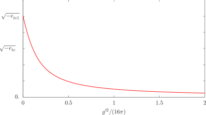
Figure 6: Variation of the square-root of the binding energy as a function of $g^{\prime 2}/(16\pi)$. The value of $-e_{tc1}$ $(\equiv-E_{tc1}/(2m_{r}))$ has been fixed at 0.01.

Of particular interest are the weak- and strong-coupling limits in $g^{\prime}$, determined by the comparison of the factors $g^{\prime 2}/(16\pi)$ and $\sqrt{-4e_{tc1}}$. In the first case, $g^{\prime 2}/(16\pi)\ll\sqrt{-4e_{tc1}}$, $-e_{tc}$ is obtained close to $-e_{tc1}$ with a small negative shift. In the second case, $g^{\prime 2}/(16\pi)\gg\sqrt{-4e_{tc1}}$, one obtains

$$\sqrt{-e_{tc}}\simeq-e_{tc1}\,\frac{16\pi}{g^{\prime 2}}.$$ (51)

(This expression could also be obtained directly from (49) by neglecting in it $e_{tc}$ in front of $e_{tc1}$.) Because of the nonlinear relationship between $e_{tc}$ and $e_{tc1}$, there appears a strong decrease in $e_{tc}$. One has

$$\frac{e_{tc}}{e_{tc1}}=-e_{tc1}\,\Big{(}\frac{16\pi}{g^{\prime 2}}\Big{)}^{2}.$$ (52)

Considering for example $-E_{tc1}\simeq 20$ MeV and $2m_{r}\simeq 2$ GeV, one has $-E_{tc1}/(2m_{r})\simeq 0.01$; values of $g^{\prime 2}/(16\pi)$ of the order of or greater than 0.5 produce ratios $E_{tc}/E_{tc1}\leq 0.04$, or equivalently $-E_{tc}\leq 0.8$ MeV. These values of $g^{\prime 2}/(16\pi)$ are not exceptional and we may conclude that we are not in the presence of a fine tuning effect. There is a nonnegligible probability, in many physical cases, to meet such a situation.

The contribution of the tetraquark state, in the $s$-channel, to the two-meson elastic scattering amplitude is obtained by inserting the tetraquark propagator between two tetraquark-two-meson couplings, as shown in Fig. 7.

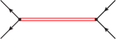
Figure 7: The tetraquark contribution, in the $s$-channel, to the two-meson elastic scattering amplitude.

One finds

$$\mathcal{T}=-\frac{(m_{1}+m_{2})^{2}g^{\prime 2}}{s-m_{tc1}^{2}+i(m_{1}+m_{2})^{2}g^{\prime 2}J^{\mathrm{r}}(s)}.$$ (53)

Proceeding as in the molecular case [Eq. (28)], one can obtain the physical coupling constant $g_{TM_{1}M_{2}}$ of the tetraquark to the two mesons:

$$g_{TM_{1}M_{2}}^{2}=32\pi\sqrt{-e_{tc}}\ \frac{1}{\Big{[}1+2\Big{(}\frac{16\pi}{g^{\prime 2}}\Big{)}^{2}(e_{tc}-e_{tc1})\Big{]}}.$$ (54)

Comparing this expression with (42), one obtains $Z$:

$$Z=\frac{1}{1+\Big{(}\frac{g^{\prime 2}}{16\pi}\Big{)}^{2}\frac{1}{2(e_{tc}-e_{tc1})}},$$ (55)

which, after taking into account Eq. (49), can also be expressed as

$$Z=\frac{\sqrt{-e_{tc}}}{\sqrt{-e_{tc}}+\frac{1}{2}\frac{g^{\prime 2}}{16\pi}}.$$ (56)

One notices, in particular from (55), that $Z$ decreases in the strong-coupling limit and takes small values. With the numerical example considered above, one has $Z\leq 0.075$. On the other hand, in the same limit, the physical coupling constant $g_{TM_{1}M_{2}}$ also decreases, like $\sqrt{-e_{tc}}$. The variation of $Z$ as a function of $g^{\prime 2}/(16\pi)$, taking into account (50), is represented in Fig. 8. One notices the rapid decrease of $Z$.

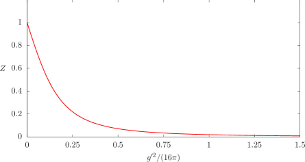
Figure 8: Variation of $Z$ as a function of $g^{\prime 2}/(16\pi)$; $-e_{tc1}$ has been fixed at 0.01.

It is also possible to calculate from (53), as in the molecular case [Eqs. (31)-(32)], the scattering length and the effective range. One finds, neglecting other contributions to the scattering amplitude,

$$a=\Big{(}\frac{g^{\prime 2}}{16\pi}\Big{)}\,\Big{(}\frac{1}{2m_{r}(-e_{tc1})}\Big{)},\ \ \ \ \ \ \ r_{e}=\frac{1}{m_{r}}\Big{(}-\frac{16\pi}{g^{\prime 2}}+\frac{2}{\pi}(1-d)\Big{)}.$$ (57)

($d$ is defined in (32).) Eliminating $g^{\prime 2}/(16\pi)$ and $e_{tc1}$ in favor of $Z$ and $e_{tc}$, one obtains the expected expressions

$$a=\frac{2(1-Z)}{(2-Z)}R,\ \ \ \ \ \ \ r_{e}=-\frac{Z}{(1-Z)}R,\ \ \ \ \ \ \ R=\frac{1}{2m_{r}}\sqrt{\frac{1}{-e_{tc}}}.$$ (58)

(The second term in $r_{e}$, which is small, has been neglected.)

It is of importance to have a precise interpretation of the values of $Z$. When $g^{\prime}=0$, $Z=1$ and the tetraquark is completely decoupled from the two mesons. This would mean that either its mass scale or quark content are different from those of the two mesons. In the opposite case, corresponding to the strong-coupling limit, $Z$ decreases and approaches the value 0. This does not mean, however, that the tetraquark’s nature becomes molecular. Nowhere, in the present model, did we consider direct interactions between mesons; the existence of the bound state is entirely due to the confining forces that are responsible of its compact nature. The value of $(1-Z)$ simply reflects the strength of the (bare, but finite) coupling of the tetraquark to the two meson clusters. As $g^{\prime}$ grows, the latter, through the radiative corrections, plays, in the internal structure of the tetraquark, an increasingly determinant role, leading to a strong decrease of the binding energy and to a corresponding increase of the radius $R$ [Eq. (58)]. The tetraquark, though of compact nature, is gradually deformed into a molecular-type state.

V.3 Resonances

A resonance may occur when the renormalized (real) mass of the compact tetraquark [Eq. (47)] lies above the two-meson threshold. Its nonrelativistic energy, defined in (45), is now positive. The position of the complex mass of the possibly existing resonance can be searched for with the same method and the same approximations as in the bound state case. Designating by $E_{TR}$ the nonrelativistic (complex) energy of the tetraquark resonance, the equivalent of Eq. (49) is

$$(e_{TR}-e_{tc1})+i\frac{g^{\prime 2}}{16\pi}\sqrt{e_{TR}}=0.$$ (59)

Its solutions are

$$\sqrt{e_{TR}}=-\frac{i}{2}\frac{g^{\prime 2}}{16\pi}\pm\sqrt{e_{tc1}-\frac{1}{4}\Big{(}\frac{g^{\prime 2}}{16\pi}\Big{)}^{2}}.$$ (60)

The imaginary part of $\sqrt{e_{TR}}$ comes out negative, which means that the two solutions lie in the second Riemann sheet. The expression of $e_{TR}$ is

$$e_{TR}=\Big{[}e_{tc1}-\frac{1}{2}\Big{(}\frac{g^{\prime 2}}{16\pi}\Big{)}^{2}\Big{]}\mp i\frac{g^{\prime 2}}{16\pi}\sqrt{e_{tc1}-\frac{1}{4}\Big{(}\frac{g^{\prime 2}}{16\pi}\Big{)}^{2}}.$$ (61)

The two solutions are complex conjugate to each other, the resonance corresponding to the negative imaginary part. One verifies that the modulus of $e_{TR}$ is equal to $e_{tc1}$:

$$|e_{TR}|=e_{tc1}.$$ (62)

The condition of the positivity of the real part of $e_{TR}$ (resonance above the threshold) requires that

$$\Big{(}\frac{g^{\prime 2}}{16\pi}\Big{)}^{2}\leq 2\,e_{tc1}.$$ (63)

This means that one is rather in the weak-coupling regime. As the coupling constant increases, the real part of the resonance energy approaches the threshold, the upper bound of (63) corresponding to its merging with the threshold. On the other hand, the imaginary part remains always different from zero; at threshold, it is only the latter that survives.

The scattering amplitude, due to the resonance, is

$$\mathcal{T}=-\frac{(m_{1}+m_{2})}{4m_{r}}\ \frac{g^{\prime 2}}{\Big{(}e-e_{tc1}+i\,\frac{g^{\prime 2}}{16\pi}\sqrt{e}\Big{)}}.$$ (64)

We have represented, in Fig. 9, the shape of $|\mathcal{T}|^{2}$ in the vicinity of the threshold, for real $E$ and for several values of $g^{\prime 2}/(16\pi)$ in its allowed domain.

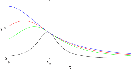
Figure 9: The shape of $|\mathcal{T}|^{2}$ for several values of $g^{\prime 2}/(16\pi)$: $\Big{(}g^{\prime 2}/(16\pi)\Big{)}^{2}/e_{tc1}=$ 0.1 (black curve), 0.75 (green), 1.25 (red), 2.0 (blue).

Expanding $\mathcal{T}$ around $E_{TR}$ [Eq. (61)] and using for the resonance the plus sign in (60), one obtains

$$\mathcal{T}\simeq-\frac{(m_{1}+m_{2})g_{TM_{1}M_{2}}^{2}}{2(E-E_{TR})},$$ (65)

with

$$g_{TM_{1}M_{2}}^{2}=\frac{32\pi\sqrt{e_{TR}}}{\sqrt{4e_{tc1}\Big{(}\frac{16\pi}{g^{\prime 2}}\Big{)}^{2}-1}}.$$ (66)

Comparing (66) with (42), the former being considered as a formal extension of the latter to the resonance region, one obtains the compositeness coefficient

$$1-Z=\frac{1}{\sqrt{4e_{tc1}\Big{(}\frac{16\pi}{g^{\prime 2}}\Big{)}^{2}-1}}.$$ (67)

We notice that, due to the inequality (63), which guarantees the occurrence of the resonance above the threshold, $(1-Z)$ is real, positive and smaller than 1. This allows us to continue giving it a probabilistic interpretation.

Writing the (reduced) energy of the resonance in the form

$$e_{TR}=e_{TRr}-i\frac{\gamma}{2},$$ (68)

where $e_{TRr}$ is the real part of the (reduced) energy and $\gamma$ the reduced dimensionless width of the resonance, defined as (see also (23))

$$\gamma\equiv\frac{\Gamma}{2m_{r}},$$ (69)

$\Gamma$ being the dimensionful width, one has from (61)

$$e_{TRr}=e_{tc1}-\frac{1}{2}\Big{(}\frac{g^{\prime 2}}{16\pi}\Big{)}^{2},\ \ \ \ \ \ \ \gamma=2\frac{g^{\prime 2}}{16\pi}\sqrt{e_{tc1}-\frac{1}{4}\Big{(}\frac{g^{\prime 2}}{16\pi}\Big{)}^{2}},$$ (70)

which allows us to express $(1-Z)$ in terms of observable quantities:

$$1-Z=\frac{\Gamma/2}{\Big{(}E_{TRr}+\sqrt{E_{TRr}^{2}+\frac{\Gamma^{2}}{4}}\Big{)}}.$$ (71)

Of particular interest is the case of narrow resonances, characterized by the inequality $\Gamma\ll 2E_{TRr}$, which entails

$$1-Z\simeq\frac{\Gamma}{4E_{TRr}},\ \ \ \ \ \ \ \Gamma\ll 2E_{TRr}.$$ (72)

It is evident from this result that the narrow resonance case favors values of $Z$ close to 1, that is, dominance of the compact nature of the tetraquark. In the opposite case, when the inequality (63) is saturated, one has vanishing of $e_{TRr}$ and merging of the resonance with the threshold, with $Z=0$; the trace of the compact origin of the resonance is then completely lost.

The expressions of the scattering length and the effective range are the same as in Eqs. (57), except that $e_{tc1}$ is now positive:

$$a=-\frac{g^{\prime 2}}{16\pi}\,\frac{1}{2m_{r}e_{tc1}}=-\frac{1}{2m_{r}}\frac{\gamma/\sqrt{2}}{\sqrt{e_{TRr}^{2}+\frac{\gamma^{2}}{4}}\sqrt{e_{TRr}+\sqrt{e_{TRr}^{2}+\frac{\gamma^{2}}{4}}}},$$ (73)

$$r_{e}=-\frac{16\pi}{g^{\prime 2}}\,\frac{1}{m_{r}}=-\frac{1}{m_{r}\gamma/\sqrt{2}}\sqrt{e_{TRr}+\sqrt{e_{TRr}^{2}+\frac{\gamma^{2}}{4}}}.$$ (74)

(The second term in $r_{e}$, which is small, has been neglected.) One notices that now, as compared to the bound state case (57), both the scattering length and the effective range are negative. In terms of $a$ and $r_{e}$, the compositeness coefficient (67) takes the form

$$1-Z=\frac{1}{\sqrt{\frac{2r_{e}}{a}-1}},$$ (75)

a relation also obtained in [84]. It can be compared with Eq. (43), valid in the bound state case. In the narrow resonance case, one has the simplified expressions

$$a\simeq-\frac{1}{4m_{r}}\frac{\gamma}{e_{TRr}^{3/2}},\ \ \ \ \ \ r_{e}\simeq-\frac{2}{m_{r}}\frac{e_{TRr}^{1/2}}{\gamma}.$$ (76)

Let us also comment on the case of the strong-coupling limit, where, in particular, the inequality (63) is no longer satisfied. We have to distinguish here two cases. The first corresponds to the domain $2e_{tc1}<(g^{\prime 2}/(16\pi))^{2}<4e_{tc1}$, in which case $(1-Z)>1$ and the real part of the energy becomes negative [Eq. (70)]. This is a sign of the instability of the initial system under the influence of the two-meson clusters and might signify the disappearance of the compact tetraquark from the spectrum. The second corresponds to the domain $4e_{tc1}<(g^{\prime 2}/(16\pi))^{2}$. In that case, $\sqrt{e_{TR}}$ [Eq. (60)] becomes imaginary and $e_{TR}$ becomes real and negative, falling back in the bound-state regime. Considering then the new value of $e_{TR}$ as a starting value (equal to a new $e_{tc1}$), one continues remaining in the bound-state regime for any value of the coupling constant, as we have seen in Eq. (50) and Fig. 6. Therefore, genuine resonances may occur, in the present model, only in the weak-coupling regime, satisfying the inequality (63).

Let us notice, as a final remark, that due to the fact that the internal structure of the compact elementary particle, assumed here as being a tetraquark, was not specified, one is also entitled to apply the previous approach, when the flavor and other quantum numbers are compatible, to ordinary mesons. In that case, its field theoretic basis is even more robust. This is supported by the large-$N_{c}$ limit of QCD [92, 93, 94, 29]. In that limit, the spectrum of the theory is composed of free mesons, which are made of one quark-antiquark pair. They do not have any internal other meson clusters. Therefore, their elementary nature with respect to the other mesons is well justified. The couplings to the other mesons appear only at nonleading order in $N_{c}$, putting the clustering phenomenon at a perturbative level. This is in contrast to the multiquark case, where the clustering occurs already at leading order in $N_{c}$ and becomes even stronger in the large-$N_{c}$ limit [29]. (Cf. also Sec. VII.)

Detailed investigations about the compositeness criterion and its applicability to various tetraquark candidates, as well as to ordinary hadrons, can be found in References [95, 96, 97, 98, 99, 100, 101, 84, 102, 103, 104, 105, 106, 107, 108, 109].

VI Presence of meson-meson interactions

In the model considered in Sec. V, where the influence of the coupling of a compact tetraquark to two mesons was studied, the presence of meson-meson interactions as a background effect was not taken into account. This had the advantage of exhibiting in a clearer way the role of the aforementioned coupling on the observable properties of the tetraquark state, in particular its gradual deformation, in the strong coupling limit, towards a molecular-type object. To complete the previous study, we include, in this section, the effect of the meson-meson interaction into the dynamical process.

VI.1 The meson-meson scattering amplitude

The meson-meson interaction, in the present effective field theory description, was considered in Secs. III and IV. When a compact tetraquark state is present, its effect is first manifested through a vertex renormalization related to the coupling constant $g^{\prime}$. This is graphically represented in Fig. 10.

Figure 10: Chain of meson-one-loop radiative corrections to the tetraquark-two-meson coupling constant $g^{\prime}$. The coupling constants at the vertices are indicated. $g^{\prime}$ is accompanied by the mass factor $(m_{1}+m_{2})$.

The corresponding vertex function, denoted $\Gamma_{TM_{1}M_{2}}^{(3)}$, takes the form (cf. Eqs. (10)-(14))

$$\Gamma_{TM_{1}M_{2}}^{(3)}(s)=\frac{i(m_{1}+m_{2})g^{\prime}}{1-ihJ(s)}.$$ (77)

We have seen that the divergence contained in $J(s)$ [Eq. (12)] is absorbed by a renormalization of the coupling constant $h$, according to (13) or (14). Here, the occurrence of the same divergence necessitates a similar renormalization of $g^{\prime}$, involving, however, also $h$:

$$g^{\prime}=\frac{g^{\prime\mathrm{r}}}{1+ih^{\mathrm{r}}J^{\mathrm{div}}}.$$ (78)

Equivalently, one has the following renormalizations:

$$\frac{h}{1-ihJ(s)}=\frac{h^{\mathrm{r}}}{1-ih^{\mathrm{r}}J^{\mathrm{r}}(s)},\ \ \ \ \ \ \ \ \ \ \ \ \ \frac{g^{\prime}}{1-ihJ(s)}=\frac{g^{\prime\mathrm{r}}}{1-ih^{\mathrm{r}}J^{\mathrm{r}}(s)}.$$ (79)

These ensure the renormalization of $\Gamma_{TM_{1}M_{2}}^{(3)}$:

$$\Gamma_{TM_{1}M_{2}}^{(3)}(s)=\frac{i(m_{1}+m_{2})g^{\prime\mathrm{r}}}{1-ih^{\mathrm{r}}J^{\mathrm{r}}(s)}.$$ (80)

A second effect of the meson-meson interactions is manifested through the radiative corrections of meson-one-loop diagrams, occurring in the tetraquark propagator (cf. Fig. 5). Each loop receives radiative corrections, as represented in Fig. 11.

Figure 11: Chain of meson-one-loop radiative corrections to the one-loop diagram of the tetraquark propagator. The coupling constants at the vertices are indicated.

The chain of such diagrams can be summed and yields the full one-loop contribution, which we designate by $\Gamma_{TT}^{(2)}(s)$. One obtains

$$\Gamma_{TT}^{(2)}(s)=(m_{1}+m_{2})^{2}\frac{(ig^{\prime})^{2}J(s)}{1-ihJ(s)}.$$ (81)

These full one-loop contributions replace now the simple loop contributions of Fig. 5. The full tetraquark propagator is then given by the series of diagrams of Fig. 12.

Figure 12: The full tetraquark propagator.

One finds for the full propagator

$$D_{t}(s)=\frac{i}{s-m_{tc0}^{2}+i(m_{1}+m_{2})^{2}g^{\prime 2}J(s)/(1-ihJ(s))}.$$ (82)

Using the renormalizations given in (78) and (79), and after taking the limit $iJ^{\mathrm{div}}\rightarrow\infty$, one finds

$$D_{t}(s)=\frac{i}{s-m_{tc0}^{2}+(m_{1}+m_{2})^{2}g^{\prime\mathrm{r}2}/[h^{\mathrm{r}}(1-ih^{\mathrm{r}}J^{\mathrm{r}}(s))]}.$$ (83)

One notices that after the renormalizations of the coupling constants $h$ and $g^{\prime}$ have been realized, the radiative corrections of the tetraquark propagator are now finite. This is in contrast to the case where the meson-meson interactions had been ignored ($h=0$) and the divergence of the radiative corrections had been absorbed by the mass renormalization, while the coupling constant $g^{\prime}$ had remained finite (cf. (46) and (47)). Nevertheless, the radiative corrections in (83) contain a singularity in $h^{\mathrm{r}}$. When $h^{\mathrm{r}}\rightarrow 0$, one recovers the divergence that exists in the aforementioned case. To remedy this defect, one has to subtract that singularity from the global radiative corrections and associate it with a renormalization of the bare mass $m_{tc0}$. Designating by $m_{tc1}$ the renormalized bare mass, one has

$$m_{tc1}^{2}=m_{tc0}^{2}-\frac{(m_{1}+m_{2})^{2}g^{\prime\mathrm{r}2}}{h^{\mathrm{r}}}.$$ (84)

As long as $h^{\mathrm{r}}$ is nonzero, this mass renormalization is finite. When $h^{\mathrm{r}}\rightarrow 0$, one recovers the situation of Eq. (47).

The full tetraquark propagator takes now the following form:

$$D_{t}(s)=\frac{i}{s-m_{tc1}^{2}+i(m_{1}+m_{2})^{2}g^{\prime\mathrm{r}2}J^{\mathrm{r}}(s)/(1-ih^{\mathrm{r}}J^{\mathrm{r}}(s))}.$$ (85)

When $h^{\mathrm{r}}\rightarrow 0$, one also recovers the propagator (48).

The meson-meson scattering amplitude is obtained by inserting the tetraquark propagator inside two vertices of the type of (77), which are finite [Eq. (80)], and by adding the contribution generated by the contact interaction (8) [Fig. 2 and Eqs. (10) and (13)]. This is represented in Fig. 13.

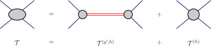
Figure 13: The meson-meson scattering amplitude, $\mathcal{T}$, due to the contributions of the renormalized compact tetraquark pole, with its renormalized vertices with two mesons, $\mathcal{T}^{(g^{\prime},h)}$, and the chain of contact interactions of Fig. 2, $\mathcal{T}^{(h)}$.

One obtains

$$\mathcal{T} \equiv \mathcal{T}^{(g^{\prime},h)}+\mathcal{T}^{(h)}$$ (86)

$$= -\frac{(m_{1}+m_{2})^{2}g^{\prime\mathrm{r}2}}{(1-ih^{\mathrm{r}}J^{\mathrm{r}}(s))^{2}}\ \frac{1}{\Big{[}s-m_{tc1}^{2}+i(m_{1}+m_{2})^{2}g^{\prime\mathrm{r}2}J^{\mathrm{r}}(s)/(1-ih^{\mathrm{r}}J^{\mathrm{r}}(s))\Big{]}}$$

$$\ \ \ \ \ \ +\frac{h^{\mathrm{r}}}{(1-ih^{\mathrm{r}}J^{\mathrm{r}}(s))}$$

$$= \frac{h^{\mathrm{r}}(s-m_{tc1}^{2})-(m_{1}+m_{2})^{2}g^{\prime\mathrm{r}2}}{\Big{[}(s-m_{tc1}^{2})(1-ih^{\mathrm{r}}J^{\mathrm{r}}(s))+i(m_{1}+m_{2})^{2}g^{\prime\mathrm{r}2}J^{\mathrm{r}}(s)\Big{]}}$$

The above expression could also have been obtained by starting from the integral equation $i\mathcal{T}=K+iKJ\mathcal{T}$, with the kernel $K$ given by

$$K=-i\frac{(m_{1}+m_{2})^{2}g^{\prime 2}}{(s-m_{tc0}^{2})}+ih.$$ (87)

After the renormalizations of the coupling constants and of the mass $m_{tc0}$ are done, one finds (86).

VI.2 Bound states

The singularities of the scattering amplitude (86) are the same as those of the tetraquark propagator (85). The separate molecular-type singularity, present in $\mathcal{T}^{(h)}$, has been cancelled by a similar singularity resulting from the radiative corrections in $\mathcal{T}^{(g^{\prime},h)}$.

We first focus on the bound state problem. The tetraquark mass, $m_{t}$, is given by the equation

$$(s_{t}-m_{tc1}^{2})(1-ih^{\mathrm{r}}J^{\mathrm{r}}(s_{t}))+i(m_{1}+m_{2})^{2}g^{\prime\mathrm{r}2}J^{\mathrm{r}}(s_{t})=0,$$ (88)

where $s_{t}=m_{t}^{2}$. Sticking to the nonrelativistic limit and using definitions similar to (22) and (23), and

$$E_{t}=m_{t}-(m_{1}+m_{2}),\ \ \ \ \ \ \ e_{t}\equiv\frac{E_{t}}{2m_{r}},$$

$$E_{tc1}=m_{tc1}-(m_{1}+m_{2}),\ \ \ \ \ \ \ e_{tc1}\equiv\frac{E_{tc1}}{2m_{r}},$$ (89)

Eq. (88) reduces to (omitting henceforth the renormalization label r from the coupling constants)

$$(-e_{t}+e_{tc1})(1+\frac{\alpha h}{16\pi}\sqrt{-e_{t}})+\frac{g^{\prime 2}}{16\pi}\sqrt{-e_{t}}=0,$$ (90)

where $\alpha$ is defined in (24). We notice that in case $g^{\prime}=0$ (absence of tetraquark-two-meson coupling), the equation splits into two independent equations yielding the molecular-type solution (24) (for $h<0$), on the one hand, and the bare compact tetraquark mass (84), on the other. In case $h=0$ (absence of molecular-type forces), the equation reduces to that of the compact tetraquark case (49). Equation (90) cannot be solved analytically, but accurate analytic approximate solutions can be found for it. One has to distinguish two cases, according to the sign of $h$.

We first consider the case $h>0$. According to the empirical relationship (26) and Fig. 3, this case corresponds to subcritical values of three-meson coupling constants, for which no genuine molecular-type bound states can exist. Even though $h$ may take large values, approaching $+\infty$, one may characterize this domain as globally representing a weak-coupling regime. One therefore expects that the tetraquark bound state originates entirely from a compact configuration, the molecular forces mainly introducing deformations.

A leading approximate solution to (90) is

$$\sqrt{-e_{t0}}=\frac{1}{2}\Big{[}-b^{\prime}+\sqrt{b^{\prime 2}-4e_{tc1}}\Big{]},\ \ \ \ \ \ \ b^{\prime}=\frac{g^{\prime 2}}{16\pi}\frac{1}{(1+\frac{\alpha h}{16\pi}\sqrt{-e_{tc1}})},$$ (91)

which generalizes (50). This expression, together with its next-to-leading term, which is presented in the Appendix A [Eq. (109)], reproduces the behavior of the exact solution with an error of less than a few percent, the error slightly increasing with $h$. The behavior of $\sqrt{-e_{t}}$ with respect to variations of $g^{\prime 2}/(16\pi)$, for fixed $h$, is similar to that of Fig. 6. With increasing $g^{\prime 2}/(16\pi)$, $\sqrt{-e_{t}}$ approaches zero, starting from $\sqrt{-e_{tc1}}$. The effect of the presence of $h$ is simply the weakening of the slope of the decrease; the molecular forces appear as opposed to the rapidity of the decrease. Fig. 14 displays the variation of $\sqrt{-e_{t}}$ for a few typical values of $\alpha h/(16\pi)$.

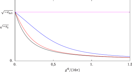
Figure 14: Variation of the square-root of the binding energy as a function of $g^{\prime 2}/(16\pi)$, for four different positive values of $\alpha h/(16\pi)$: $0$ (black curve), $5$ (red), $30$ (blue), $+\infty$ (magenta, the horizontal line at $\sqrt{-e_{tc1}}$); $-e_{tc1}$ has been fixed at 0.01.

The second case to be considered is $h<0$. Here, we have two distinct solutions, which we shall label with the indices 1 and 2, corresponding to the generalizations of the two solutions existing in the uncoupled case with $g^{\prime}=0$. In the present domain of $h$, the most interesting case corresponds to large values of $-h$, producing a molecular-type state near the two-meson threshold. The case where $-h$ is small, actually corresponds, according to Fig. 3, to large values of the three-meson coupling constant $g$, which lies outside the domain of applicabilty of the nonrelativistic approximation. Hence, we shall stick to a single large value of $-h$, fixed for numerical applications at $-\alpha h/(16\pi)=10^{3/2}=31.62$, for $-e_{tc1}=0.01$, and also shall consider its limiting value $+\infty$.

The first solution describes the evolution of the molecular-type solution (24) under the influence of the coupling $g^{\prime}$. A leading approximate expression of it is

$$\sqrt{-e_{t0,(1)}}=-\frac{e_{tc1}}{\frac{g^{\prime 2}}{16\pi}+e_{tc1}\frac{\alpha h}{16\pi}}.$$ (92)

Its next-to-leading term is given in the Appendix A. The analytic approximation (110) reproduces the behavior of the exact solution with an error of less than one per mil. The behavior of $\sqrt{-e_{t,(1)}}$ with respect to variations of $g^{\prime 2}/(16\pi)$, for fixed $h$, is again similar to that of Fig. 6; however, now, it starts, when $g^{\prime 2}/(16\pi)=0$, from $\sqrt{-e_{tm}}$ [Eq. (24)], instead of $\sqrt{-e_{tc1}}$ (Fig. 15). In the limit $h\rightarrow-\infty$, $\sqrt{-e_{tm}}$ tends to $0$ (the two-meson threshold) and the whole curve coincides with the horizontal $0$ line.

The second solution describes the change of the compact-type solution (50) under the influence of the coupling $h$. A leading approximate expression of it is

$$\sqrt{-e_{t0,(2)}}=\sqrt{-e_{tc1}-\frac{g^{\prime 2}/(16\pi)}{\alpha h/(16\pi)}}.$$ (93)

(The condition $-\frac{\alpha h}{16\pi}\sqrt{-e_{t0,(2)}}\gg 1$ should be fulfilled.) Its next-to-leading term is given in the Appendix A. The analytic approximation (111) reproduces the behavior of the exact solution with an error of less than one per cent. The behavior of $\sqrt{-e_{t,(2)}}$ with respect to variations of $g^{\prime 2}/(16\pi)$, for fixed $h$, is represented by an increasing function. The binding energy of the compact tetraquark thus increases in the presence of the molecular-type state (Fig. 15). In the limit $h\rightarrow-\infty$ the curve coincides with the horizontal $\sqrt{-e_{tc1}}$ line. Actually, the solution $\sqrt{-e_{t,(2)}}$ can be considered as the continuation of the solution found in the case of positive values of $h$ to negative values of $h$. As can be seen in Fig. 14, when $h$ increases with positive values, the solution reaches, in the limit $h\rightarrow+\infty$, the constant value $\sqrt{-e_{tc1}}$. Then, according to Fig. 3, $h$ passes to $-\infty$, which also corresponds, for the solution $\sqrt{-e_{t,(2)}}$, to the same constant value $\sqrt{-e_{tc1}}$ in Fig. 15. The increasing of $h$ with negative values then produces the curves lying above that horizontal line.

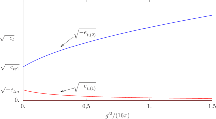
Figure 15: The two solutions of the bound state equation (90) and their variation under changes of $g^{\prime 2}/(16\pi)$. The value of $-\alpha h/(16\pi)$ has been fixed at $31.62$ and that of $-e_{tc1}$ at $0.01$. At the limiting value $h=-\infty$, $\sqrt{-e_{t,(1)}}$ coincides with the horizontal line $0$, while $\sqrt{-e_{t,(2)}}$ coincides with the horizontal line $\sqrt{-e_{tc1}}$.

Expanding the scattering amplitude (86) around the bound state pole (cf. (28)), one obtains the physical coupling constant $g_{TM_{1}M_{2}}$, expressed in two equivalent ways, using (90):

$$g_{TM_{1}M_{2}}^{2}=\frac{32\pi\sqrt{-e_{t}}}{\Big{[}1+\frac{2g^{\prime 2}}{16\pi}\frac{(-e_{t})^{3/2}}{(e_{t}-e_{tc1})^{2}}\Big{]}}=\frac{32\pi\sqrt{-e_{t}}}{\Big{[}1+\frac{2\sqrt{-e_{t}}}{g^{\prime 2}/(16\pi)}\Big{(}1+\frac{\alpha h}{16\pi}\sqrt{-e_{t}}\Big{)}^{2}\Big{]}}.$$ (94)

Comparison of these expressions with (42) yields $Z$:

$$Z=\frac{\frac{2g^{\prime 2}}{16\pi}(-e_{t})^{3/2}}{(e_{t}-e_{tc1})^{2}+\frac{2g^{\prime 2}}{16\pi}(-e_{t})^{3/2}}=\frac{\Big{(}1+\frac{\alpha h}{16\pi}\sqrt{-e_{t}}\Big{)}^{2}\sqrt{-e_{t}}}{\Big{(}1+\frac{\alpha h}{16\pi}\sqrt{-e_{t}}\Big{)}^{2}\sqrt{-e_{t}}+\frac{1}{2}\frac{g^{\prime 2}}{16\pi}},$$ (95)

which is manifestly a positive quantity bounded by 1.

The value of $Z$ and its behavior under variations of the coupling constants depend on the specific bound states that we have met above. When $h>0$, we have one bound state with the square-root of the binding energy having the approximate expressions (90) and (109). For this case, the qualitative features of $Z$ are more transparent in the second expression of (95). When $g^{\prime}\rightarrow 0$, for fixed $h$, $\sqrt{-e_{t}}\rightarrow\sqrt{-e_{tc1}}$ (cf. Fig. 14); then $Z\rightarrow 1$. When $g^{\prime}$ increases, $\sqrt{-e_{t}}$ decreases rapidly and tends to zero. The behavior of $Z$ remains very similar to that of Fig. 8, with the difference that the presence of $h$ slows down the decrease of $Z$. We display, in Table 1, the values of $Z$ for several values of $\alpha h/(16\pi)$, for $g^{\prime 2}/(16\pi)=0.5$ and $-e_{tc1}=0.01$.

Table 1: Values of $Z$, for several positive values of $\alpha h/(16\pi)$ (Fig. 14), for $g^{\prime 2}/(16\pi)=0.5$ and $-e_{tc1}=0.01$.

$\alpha h/(16\pi)$	0	1.	5.	30.	$\infty$
$Z$	0.072	0.075	0.094	0.388	1.

When $h<0$, we have two bound states with the square-root of the binding energies having the approximate expressions (92) and (110), on the one hand, and (93) and (111), on the other. For the solution 1, $\sqrt{-e_{t}}$ remains much smaller than $\sqrt{-e_{tc1}}$ (cf. Fig. 15); in that case, the first expression of $Z$ in (95) is more adequate for the analysis. When $g^{\prime}\rightarrow 0$, $Z\rightarrow 0$. However, the evolution of $Z$ under variations of $g^{\prime}$ is no longer monotonic. For fixed $h$, $Z$ increases, starting from zero at $g^{\prime}=0$, reaches a maximum value nearly at $g^{\prime 2}/(16\pi)=e_{tc1}\alpha h/(32\pi)$ ($\simeq 0.16$ for $\alpha h/(16\pi)=-31.62$ and $-e_{tc1}=0.01$), then decreases down to 0. The bound state remains, therefore, very close to a molecular configuration in all the interval of variation of $g^{\prime}$. The main influence of the latter is reflected in the continuous decrease of the binding energy, accentuating the shallowness of the state. We display, in Table 2, for $\alpha h/(16\pi)$ fixed at $-31.62$, with $-e_{tc1}=0.01$, the values of $Z$ for several values of $g^{\prime 2}/(16\pi)$.

Table 2: Values of $Z$, corresponding to solution 1 of Fig. 15, for several values of $g^{\prime 2}/(16\pi)$, for $\alpha h/(16\pi)=-31.62$, with $-e_{tc1}=0.01$.

$g^{\prime 2}/(16\pi)$	0	0.1	0.16	0.25	0.5	1.	1.5	$\infty$
$Z$	0	0.029	0.030	0.027	0.018	0.008	0.005	0.

For the solution 2, the second expression of $Z$ in (95) is more adequate for the analysis. When $g^{\prime}\rightarrow 0$, $Z\rightarrow 1$ (the factor $(1+\alpha h/(16\pi)\sqrt{-e_{t}})$ does not vanish). When $g^{\prime}$ increases, $Z$ decreases, reaches a minimum value nearly at $g^{\prime 2}/(16\pi)=2e_{tc1}\alpha h/(16\pi)$ ($\simeq 0.6$ for $\alpha h/(16\pi)=-31.62$ and $-e_{tc1}=0.01$), then increases up to 1. The bound state remains very close to the compact configuration in all the interval of variation of $g^{\prime}$. The main influence of the latter is reflected in the continuous increase of the binding energy (Fig. 15). We display, in Table 3, for $\alpha h/(16\pi)$ fixed at $-31.62$, with $-e_{tc1}=0.01$, the values of $Z$ for several values of $g^{\prime 2}/(16\pi)$.

Table 3: Values of $Z$, corresponding to solution 2 of Fig. 15, for several values of $g^{\prime 2}/(16\pi)$, for $\alpha h/(16\pi)=-31.62$, with $-e_{tc1}=0.01$.

$g^{\prime 2}/(16\pi)$	0	0.1	0.25	0.5	1.	1.5	$\infty$
$Z$	1.	0.948	0.933	0.930	0.937	0.943	1.

To determine the scattering length and the effective range, one expresses the scattering amplitude $\mathcal{T}$ in the scattering region $E>0$:

$$\mathcal{T}=8\pi(m_{1}+m_{2})\,\Big{[}\,\frac{32\pi(e-e_{tc1})m_{r}}{(e-e_{tc1})\alpha h-g^{\prime 2}}+\frac{(1-d)k^{2}}{\pi m_{r}}-ik\,\Big{]}^{-1},$$ (96)

from which one deduces, with the aid of (33) and (34),

$$a=\frac{1}{2m_{r}}\Big{(}-\frac{\alpha h}{16\pi}-\frac{1}{e_{tc1}}\frac{g^{\prime 2}}{16\pi}\Big{)},\ \ \ \ \ \ r_{e}=-\frac{1}{m_{r}}\frac{g^{\prime 2}/(16\pi)}{\Big{(}\frac{\alpha h}{16\pi}e_{tc1}+\frac{g^{\prime 2}}{16\pi}\Big{)}^{2}}+\frac{1}{m_{r}}\frac{2}{\pi}(1-d),$$ (97)

where $d$ is defined in (32) and $\alpha$ in (24). The relationship of $a$ and $r_{e}$ with $Z$ [Eq. (95)] is not, however, as simple as in the previous cases [Eqs. (41) and (73)]. The reason for this comes from the fact that $\mathcal{T}$ contains now a zero in the vicinity of the bound state pole and does not satisfy Weinberg’s representation (44) [89, 110]. For $h>0$, the zero occurs in the domain $e>e_{tc1}$, while for $h<0$, it occurs in the domain $e<e_{tc1}$. Nevertheless, expressions (97) are simple enough in terms of the elementary parameters of the theory, and together with the knowledge of the binding energy, if they are measured experimentally or on the lattice, allow the calculation of $Z$. In particular, the presence of the coupling $g^{\prime}$ between the tetraquark and the two mesons provides $r_{e}$ in general with a negative value, whatever the sign of $h$ is. We notice that for $h<0$, $a$ is positive, as it receives contributions from two independent bound states. For $h>0$, $a$ is positive for $\alpha h<-g^{\prime 2}/e_{tc1}$ and negative for $\alpha h>-g^{\prime 2}/e_{tc1}$. For $\alpha h=-g^{\prime 2}/e_{tc1}$, $a$ vanishes and simultaneously $r_{e}$ tends to $-\infty$. For $g^{\prime 2}/(16\pi)=0.5$ and $-e_{tc1}=0.01$, the latter critical value of $h$ occurs at $\alpha h/(16\pi)=50$. (Cf. (26) for its conversion into a three-meson coupling constant $\overline{g}$; the latter lies slightly below the critical value $\overline{g}_{\mathrm{cr}}$ displayed in (7).)

VI.3 Resonances

Resonances may occur when the renormalized (real) compact tetraquark mass, given by (84), lies above the two-meson threshold. In that case, the nonrelativistic energy $E_{tc1}$ of (VI.2) is positive. The poles of the scattering amplitude (86) may have complex values. Designating by $E_{TR}$ the complex energy of the pole, the equivalent of Eq. (90) is now

$$(e_{TR}-e_{tc1})(1-i\frac{\alpha h}{16\pi}\sqrt{e_{TR}})+i\frac{g^{\prime 2}}{16\pi}\sqrt{e_{TR}}=0.$$ (98)

When $h\neq 0$, this equation has to be solved numerically. Introducing the definitions

$$\sqrt{e_{TR}}=u+i\,v,\ \ \ \ e_{TR}=u^{2}-v^{2}+i\,2uv\equiv e_{TRr}+i\,e_{TRi},\ \ \ \ \ \ u,v\ \mathrm{real},$$ (99)

where $e_{TRr}$ and $e_{TRi}$ are the real and imaginary parts of $e_{TR}$, respectively, one can study the behavior of $e_{TR}$ under variations of $g^{\prime 2}$ and $h$. The physical conditions to be imposed on the solutions are $v<0$, $e_{TRi}<0$ and $e_{TRr}>0$ (the resonance lies above the two-meson threshold). In the case $h=0$, the upper bound (63) had been found for $g^{\prime 2}/(16\pi)$.

When $h\neq 0$, one has to distinguish two main domains of $h$ (cf. Fig. 3): (i) $h>0$ and small, corresponding to the weak-coupling regime of the meson-meson interaction; (ii) $|h|$ large, corresponding to the strong-coupling regime, with the possibility of existence of a genuine molecular-type bound state (for $h<0$). In the first case, the qualitative behavior of the solutions is naturally close to that of the case with $h=0$, studied in Sec. V, the only changes being small quantitative ones. Thus, for $h/(16\pi)\leq 0.2/\sqrt{-e_{tc1}}$, a conservative upper bound for $g^{\prime 2}$ is $g^{\prime 2}/(16\pi)\leq\sqrt{-e_{tc1}}$. When $g^{\prime 2}$ increases from 0 to its upper bound, the resonance approaches the two-meson threshold with its imaginary part remaining finite, but relatively decreasing. In the second case, for the same variation of $g^{\prime 2}$, the resonance approches the threshold for $h<0$ and moves away from it for $h>0$. There are also regions of $h$ for which large values of $g^{\prime 2}$ are possible, however they are not obtained by continuous variations of all interactions.

For completeness, we display here the equation satisfied by the imaginary part of $\sqrt{e_{TR}}$:

$$v=-\frac{1}{2}\,\frac{g^{\prime 2}}{16\pi}\,\frac{1}{\Big{(}1+2v\frac{\alpha h}{16\pi}+(\frac{\alpha h}{16\pi})^{2}|e_{TR}|\Big{)}},$$ (100)

$|e_{TR}|$ being the modulus of $e_{TR}$, which generally favors negative values of $v$ (when $h<0$ or when $h>0$ but small).

Expanding $\mathcal{T}$ [Eq. (86)] around $E_{TR}$, as in (65), one obtains the expression of the tetraquark-two-meson coupling constant squared:

$$g_{TM_{1}M_{2}}^{2}=32\pi\sqrt{e_{TR}}\,\frac{g^{\prime 2}/(16\pi)}{\Big{[}2\sqrt{e_{TR}}\Big{(}1-i\frac{\alpha h}{16\pi}\sqrt{e_{TR}}\Big{)}^{2}+i\frac{g^{\prime 2}}{16\pi}\Big{]}}.$$ (101)

Generally, the multiplicative factor accompanying $32\pi\sqrt{e_{TR}}$ is identified with the compositeness coefficient $(1-Z)$ [Eqs. (42), (67), (95)]. Here, however, the corresponding coefficient is complex when $h\neq 0$ and, therefore, a probabilistic interpretation of it is no longer possible (cf. also [100, 101]). A natural extension of the usual definition would correspond to taking the modulus of the corresponding expression as being equivalent to $(1-Z)$. While such an extension would ensure the reality condition of the probability candidate, it does not yet guarantee its boundedness by 1. Indeed, one may check that when the coupling constant $g^{\prime 2}$ exceeds its upper bound, mentioned earlier in this subsection, one finds, for small positive values of $h$, that $(1-Z)$ exceeds 1. Such a situation has also been found in Sec. V.3 and has been interpreted as a sign of the instability of the initial system, leading to the disappearance of the compact tetraquark from the spectrum. On the other hand, large values of $g^{\prime 2}$ generally send back the resonance to the bound state domain. We therefore adopt the modulus prescription, with the restriction that $g^{\prime 2}$ respects its upper bound:

$$(1-Z)=\Big{|}\frac{g^{\prime 2}/(16\pi)}{\Big{[}2\sqrt{e_{TR}}\Big{(}1-i\frac{\alpha h}{16\pi}\sqrt{e_{TR}}\Big{)}^{2}+i\frac{g^{\prime 2}}{16\pi}\Big{]}}\Big{|}.$$ (102)

The general properties of $Z$ are then similar to those met in the case $h=0$. When the resonance approaches the two-meson threshold, $Z$ tends to 0, while when the resonance stays in the vicinity of its primary position, this mainly corresponding to small values of $g^{\prime 2}$, $Z$ remains close to 1. On the other hand, large and negative values of $h$ have the tendency to push the resonance towards the two-meson threshold, while large and positive values of $h$ repel the resonance from the threshold.

It is worthwile recalling that in the case $h<0$, the spectrum also contains a molecular-type bound state, whose binding energy has been approximately estimated, in the two-bound-state case, by means of Eq. (92), where $e_{tc1}<0$. The same formula could also be used for the evaluation of the binding energy in the resonance case, where now $e_{tc1}>0$:

$$\sqrt{-e_{t0,(1)}}=\frac{1}{\Big{(}-\frac{\alpha h}{16\pi}-\frac{g^{\prime 2}}{16\pi e_{tc1}}\Big{)}}.$$ (103)

We find that the bound state exists only when $-{\alpha h}/(16\pi)$ is greater than ${g^{\prime 2}}/(16\pi e_{tc1})$; the condition of the vicinity of the bound state to the two-meson threshold actually requires much larger values. For instance, with $e_{tc1}=0.01$ and ${g^{\prime 2}}/(16\pi)=0.1$, one would need $-{\alpha h}/{16\pi}>10$. Values of $-{\alpha h}/{16\pi}$ of the order of 30, which were frequently considered throughout the present work, would then produce a binding energy $-e_{t0,(1)}$ of the order of 0.0025.

The expressions of the scattering length and the effective range are the same as in Eqs. (97), with the only difference that $e_{tc1}$ is now positive. The contribution of the term proportional to $g^{\prime 2}$ in $a$ is now negative and in the case $h<0$ the same competition as in the case of the bound-state binding energy (103) arises between the contributions of $h$ and $g^{\prime 2}$. In case $-\alpha h/(16\pi)-g^{\prime 2}/(16\pi e_{tc1})$ is negative, the bound state disappears and the scattering length becomes negative. While the effective range is insensitive to the sign of that combination, it nevertheless has a singularity when the latter vanishes.

In summary, the existence of resonances is much sensitive to the strength of the primary (bare) tetraquark-two-meson coupling constant, which should remain sufficiently weak. Large values of it generally resend the resonance to the bound state region. There is also an interval of the coupling constant for which the tetraquark may disappear from the spectrum. This is in contrast to the bound state case, where all values of the coupling constant are acceptable, with different consequences according to the values of the four-meson coupling constant.

VII Large-$N_{c}$ analysis

At large $N_{c}$, ordinary mesons are stable noninteracting particles [92, 111, 112, 93, 113, 94] and can be considered as compact objects. Their couplings to other mesons is of subleading order in $N_{c}$. Therefore, the latter can act on them only as perturbations, not affecting their compact structure.

This is not the case of tetraquarks, because of the existence of internal mesonic clusters. The compact structure of primarily existing tetraquarks is not protected by the large-$N_{c}$ limit. This is due to the fact that the interaction forces acting for the formation of mesonic clusters are $(N_{c}-1)$ times larger than the forces forming diquark compact objects [20, 29] (assuming that the confining forces have the same color structure as one-gluon exchange terms). This means that the primary coupling constant $g^{\prime}$ that connects the compact tetraquark to the two mesons should behave at large $N_{c}$ like $N_{c}^{1/2}$, assuming that the compact tetraquark state and energy are of order $N_{c}^{0}$. For the squared quantity, one has

$$g^{\prime 2}=O(N_{c}).$$ (104)

Concerning the four-meson contact-type coupling constant $h$, we have emphasized in Sec. III that it is not an elementary coupling constant and should rather be related to the three-meson coupling constants of the higher-energy theory. The latter coupling constants generically behave, at large $N_{c}$, like $N_{c}^{-1/2}$ [93, 94, 112, 29] and vanish in that limit. Compared to the critical coupling constant, introduced in (7), they lie, in the subcritical domain. Meson-meson interactions cannot, therefore, produce on their own bound states in the large-$N_{c}$ limit. Going back to the empirical formula (26), we deduce that $h$ is positive and lies in its perturbative domain, behaving like $\overline{g}^{2}$:

$$h=O(N_{c}^{-1}),\ \ \ \ \ h>0.$$ (105)

The meson-meson interaction has, therefore, only a subleading effect with respect to the direct compact-tetraquark–two-meson interaction. From Eqs. (91) and (52) one deduces that the tetraquark binding energy vanishes like $N_{c}^{-2}$:

$$-e_{tc}=O(N_{c}^{-2}).$$ (106)

From (95) and (56), one also finds the behavior of the elementariness coefficient:

$$Z=O(N_{c}^{-2}).$$ (107)

At large $N_{c}$, the compact tetraquark is thus transformed into a shallow, molecular-type, bound state.

From Eqs. (94) and (54), one deduces the behavior of the physical coupling constant $g_{TM_{1}M_{2}}$:

$$g_{TM_{1}M_{2}}^{2}=O(N_{c}^{-1}).$$ (108)

This result is in accordance with other general estimates done in the large-$N_{c}$ limit, which predict the vanishing of the coupling constant in that limit [114, 115, 116, 117, 118, 90, 91, 29]. The behavior (108) should only be considered as a generic one. The power of the decrease may slightly change according to the detailed flavor content of the tetraquark state or other more refined analyses.

Concerning the resonance states, we had found that they show up only in the weak-coupling regime. However, the large-$N_{c}$ limit imposes the strong-coupling regime. Therefore, in that limit, resonances should disappear from the spectrum, at least from the neighberhood of the two-meson threshold.

In conclusion, in the large-$N_{c}$ landscape, tetraquarks may survive only in the form of shallow, molecular-type, bound states, which are relics of primarily created compact states.

VIII Conclusion

The compact tetraquark scheme, considered in its simplest version, where diquarks and antidiquarks are separately gathered in very small volumes, can be considered as a starting point for the analysis of the tetraquark properties. In this situation, because of the dominance of the attractive confining forces, one usually finds confined bound states, in parallel to the case of ordinary hadrons. However, the very existence of underlying meson-clustering interactions in the general system forces the initial compact state to evolve towards a more complicated structure, where now molecular-type configurations are also present. In an effective field theory approach, where the compact tetraquark is represented as an elementary particle, this evolution was studied, within a scalar interaction framework, by means of the primary compact-tetraquark–two-meson coupling constant. Another quantity, more related to physical observables, is the elementariness coefficient $Z$, which varies between 1, corresponding to the pure elementary case, and 0, corresponding to the completely composite case. Stronger is the primary coupling constant, smaller is the value of $Z$. In the strong-coupling limit, the system tends to a dominant molecular configuration, characterized by a shallow structure. In the case of resonances, only the weak-coupling regime provides a stable framework for their existence. For higher values of the coupling constant, either the resonance disappears from the spectrum, or is resent to the bound state domain.

The consideration of the large-$N_{c}$ limit of QCD provides an additional support to the dominance of the strong-coupling regime of the coupling constant, with all its consequences.

Many of the tetraquark candidates, whose elementariness has been evaluated in the literature from experimental data, have led to values of $Z$ which are neither 1, nor 0. This is a clear indication of the mixture of configurations that results from the evolution described above. Nonzero values of $Z$, even small ones, are indicative of the existence of a primary compact state. Shallowness of bound states, with small values of $Z$, may receive a natural explanation as resulting from the strong-coupling limit of the interaction compact-tetraquark–meson-clusters, also supported by the large-$N_{c}$ limit of QCD.

The analysis undertaken in the present work was based on the simplest qualitative approach, considering scalar interactions, ignoring spin degrees of freedom and details of quark flavors, and using nonrelativistic limit and single-channel formalism for the meson clusters. A more general and refined quantitative analysis, concerning definite candidates, should include the missing ingredients.

*

Appendix A

We present in this appendix the approximate analytic expressions of the solutions of Eq. (90) for the two cases of $h$.

For the case $h>0$, the approximate solution, including also the next-to-leading term to (91), is

$$\sqrt{-e_{t}}\simeq\sqrt{-e_{t0}}\Big{[}1-\frac{b^{\prime}\frac{\alpha h}{16\pi}(\sqrt{-e_{tc1}}-\sqrt{-e_{t0}})}{\Big{(}\frac{g^{\prime 2}}{16\pi}-\frac{2\alpha h}{16\pi}e_{tc1}+(2-3b^{\prime}\frac{\alpha h}{16\pi})\sqrt{-e_{t0}}\Big{)}}\Big{]}.$$ (109)

For the case $h<0$, the first solution, in its approximate form, including also the next-to-leading term to (92), is

$$\sqrt{-e_{t,(1)}}\simeq\sqrt{-e_{t0,(1)}}\Big{[}1-\frac{\sqrt{-e_{t0,(1)}}(1+\frac{\alpha h}{16\pi}\sqrt{-e_{t0,(1)}})}{\Big{(}\frac{g^{\prime 2}}{16\pi}+\frac{\alpha h}{16\pi}e_{tc1}+\sqrt{-e_{t0,(1)}}(2+3\frac{\alpha h}{16\pi}\sqrt{-e_{t0,(1)}})\Big{)}}\Big{]}.$$ (110)

The second solution, in its approximate form, including also the next-to-leading term to (93), is

$$\sqrt{-e_{t,(2)}}\simeq\sqrt{-e_{t0,(2)}}-\frac{g^{\prime 2}/(16\pi)}{2\alpha h/(16\pi)}\ \frac{1}{\Big{(}\frac{g^{\prime 2}}{16\pi}+\frac{\alpha h}{16\pi}e_{tc1}-\sqrt{-e_{t0,(2)}}\Big{)}}.$$ (111)

References

- Choi et al. [2003] S. Choi et al. (Belle), Phys. Rev. Lett. 91, 262001 (2003), arXiv:hep-ex/0309032 .
- Aubert et al. [2003] B. Aubert et al. (BaBar), Phys. Rev. Lett. 90, 242001 (2003), arXiv:hep-ex/0304021 .
- Besson et al. [2003] D. Besson et al. (CLEO), Phys. Rev. D 68, 032002 (2003), [Erratum: Phys. Rev. D 75 (2007) 119908], arXiv:hep-ex/0305100 .
- Aubert et al. [2005] B. Aubert et al. (BaBar), Phys. Rev. Lett. 95, 142001 (2005), arXiv:hep-ex/0506081 .
- Ablikim et al. [2013a] M. Ablikim et al. (BESIII), Phys. Rev. Lett. 110, 252001 (2013a), arXiv:1303.5949 [hep-ex] .
- Liu et al. [2013] Z. Liu et al. (Belle), Phys. Rev. Lett. 110, 252002 (2013), [Erratum: Phys. Rev. Lett. 111 (2013) 019901], arXiv:1304.0121 [hep-ex] .
- Ablikim et al. [2013b] M. Ablikim et al. (BESIII), Phys. Rev. Lett. 111, 242001 (2013b), arXiv:1309.1896 [hep-ex] .
- Aaij et al. [2014] R. Aaij et al. (LHCb), Phys. Rev. Lett. 112, 222002 (2014), arXiv:1404.1903 [hep-ex] .
- Aaij et al. [2015] R. Aaij et al. (LHCb), Phys. Rev. Lett. 115, 072001 (2015), arXiv:1507.03414 [hep-ex] .
- Aaij et al. [2020a] R. Aaij et al. (LHCb), Sci. Bull. 65, 1983 (2020a), arXiv:2006.16957 [hep-ex] .
- Aaij et al. [2020b] R. Aaij et al. (LHCb), Phys. Rev. D 102, 112003 (2020b), arXiv:2009.00026 [hep-ex] .
- Wu [2021] L. Wu, Nucl. Part. Phys. Proc. 312-317, 15287 (2021), arXiv:2012.15473 [hep-ex] .
- Gell-Mann [1964] M. Gell-Mann, Phys. Lett. 8, 214 (1964).
- Zweig [1964] G. Zweig, in Developments in the quark theory of hadrons, vol. 1. 1964 - 1978, edited by D. Lichtenberg and S. P. Rosen (Hadronic Press, Massachusets, USA, 1980, 1964) p. 22.
- Jaffe [1977] R. L. Jaffe, Phys. Rev. D 15, 267 (1977).
- Jaffe [2008] R. L. Jaffe, Nucl. Phys. A 804, 25 (2008).
- Chen et al. [2016] H.-X. Chen, W. Chen, X. Liu, and S.-L. Zhu, Phys. Rep. 639, 1 (2016), arXiv:1601.02092 [hep-ph] .
- Hosaka et al. [2016] A. Hosaka, T. Iijima, K. Miyabayashi, Y. Sakai, and S. Yasui, PTEP 2016, 062C01 (2016), arXiv:1603.09229 [hep-ph] .
- Lebed et al. [2017] R. F. Lebed, R. E. Mitchell, and E. S. Swanson, Prog. Part. Nucl. Phys. 93, 143 (2017), arXiv:1610.04528 [hep-ph] .
- Esposito et al. [2017] A. Esposito, A. Pilloni, and A. D. Polosa, Phys. Rep. 668, 1 (2017), arXiv:1611.07920 [hep-ph] .
- Ali et al. [2017] A. Ali, J. S. Lange, and S. Stone, Prog. Part. Nucl. Phys. 97, 123 (2017), arXiv:1706.00610 [hep-ph] .
- Guo et al. [2018] F.-K. Guo, C. Hanhart, U.-G. Meissner, Q. Wang, Q. Zhao, and B.-S. Zou, Rev. Mod. Phys. 90, 015004 (2018), arXiv:1705.00141 [hep-ph] .
- Olsen et al. [2018] S. L. Olsen, T. Skwarnicki, and D. Zieminska, Rev. Mod. Phys. 90, 015003 (2018), arXiv:1708.04012 [hep-ph] .
- Karliner et al. [2018] M. Karliner, J. L. Rosner, and T. Skwarnicki, Ann. Rev. Nucl. Part. Sci. 68, 17 (2018), arXiv:1711.10626 [hep-ph] .
- Albuquerque et al. [2019] R. M. Albuquerque, J. M. Dias, K. Khemchandani, A. Martínez Torres, F. S. Navarra, M. Nielsen, and C. M. Zanetti, J. Phys. G 46, 093002 (2019), arXiv:1812.08207 [hep-ph] .
- Liu et al. [2019] Y.-R. Liu, H.-X. Chen, W. Chen, X. Liu, and S.-L. Zhu, Prog. Part. Nucl. Phys. 107, 237 (2019), arXiv:1903.11976 [hep-ph] .
- Ali et al. [2019] A. Ali, L. Maiani, and A. D. Polosa, Multiquark Hadrons (Cambridge University Press, Cambridge, UK, 2019).
- Brambilla et al. [2020] N. Brambilla, S. Eidelman, C. Hanhart, A. Nefediev, C.-P. Shen, C. E. Thomas, A. Vairo, and C.-Z. Yuan, Phys. Rep. 873, 1 (2020), arXiv:1907.07583 [hep-ex] .
- Lucha et al. [2021] W. Lucha, D. Melikhov, and H. Sazdjian, Prog. Part. Nucl. Phys. 120, 103867 (2021), arXiv:2102.02542 [hep-ph] .
- Voloshin and Okun [1976] M. B. Voloshin and L. B. Okun, JETP Lett. 23, 333 (1976), [Pisma Zh. Eksp. Teor. Fiz. 23, 369 (1976)].
- De Rújula et al. [1977] A. De Rújula, H. Georgi, and S. L. Glashow, Phys. Rev. Lett. 38, 317 (1977).
- Jaffe and Wilczek [2003] R. Jaffe and F. Wilczek, Phys. Rev. Lett. 91, 232003 (2003), arXiv:hep-ph/0307341 [hep-ph] .
- Shuryak and Zahed [2004] E. Shuryak and I. Zahed, Phys. Lett. B 589, 21 (2004), arXiv:hep-ph/0310270 [hep-ph] .
- Maiani et al. [2005a] L. Maiani, F. Piccinini, A. D. Polosa, and V. Riquer, Phys. Rev. D 71, 014028 (2005a), arXiv:hep-ph/0412098 [hep-ph] .
- Maiani et al. [2005b] L. Maiani, V. Riquer, F. Piccinini, and A. D. Polosa, Phys. Rev. D 72, 031502 (2005b), arXiv:hep-ph/0507062 [hep-ph] .
- Weinberg [1965] S. Weinberg, Phys. Rev. 137, B672 (1965).
- Törnqvist [1994] N. A. Törnqvist, Z. Phys. C 61, 525 (1994), arXiv:hep-ph/9310247 [hep-ph] .
- Weinberg [1979] S. Weinberg, Physica A 96, 327 (1979).
- Gasser and Leutwyler [1984] J. Gasser and H. Leutwyler, Annals Phys. 158, 142 (1984).
- Manohar [1997] A. V. Manohar, Perturbative and nonperturbative aspects of quantum field theory. Proceedings, 35. Internationale Universitätswochen für Kern- und Teilchenphysik: Schladming, Austria, March 2-9, 1996, Lect. Notes Phys. 479, 311 (1997), arXiv:hep-ph/9606222 [hep-ph] .
- Georgi [1990] H. Georgi, Phys. Lett. B 240, 447 (1990).
- Neubert [1994] M. Neubert, Phys. Rep. 245, 259 (1994), arXiv:hep-ph/9306320 [hep-ph] .
- Casalbuoni et al. [1997] R. Casalbuoni, A. Deandrea, N. Di Bartolomeo, R. Gatto, F. Feruglio, and G. Nardulli, Phys. Rep. 281, 145 (1997), arXiv:hep-ph/9605342 .
- Caswell and Lepage [1986] W. E. Caswell and G. P. Lepage, Phys. Lett. B 167, 437 (1986).
- Brambilla et al. [2005] N. Brambilla, A. Pineda, J. Soto, and A. Vairo, Rev. Mod. Phys. 77, 1423 (2005), arXiv:hep-ph/0410047 .
- Lucha et al. [2019] W. Lucha, D. Melikhov, and H. Sazdjian, Phys. Rev. D 100, 094017 (2019), arXiv:1908.10164 [hep-ph] .
- Dosch [1983] H. G. Dosch, Phys. Rev. D 28, 412 (1983).
- Alexandrou and Koutsou [2005] C. Alexandrou and G. Koutsou, Phys. Rev. D 71, 014504 (2005), arXiv:hep-lat/0407005 [hep-lat] .
- Okiharu et al. [2005a] F. Okiharu, H. Suganuma, and T. T. Takahashi, Phys. Rev. Lett. 94, 192001 (2005a), arXiv:hep-lat/0407001 [hep-lat] .
- Okiharu et al. [2005b] F. Okiharu, H. Suganuma, and T. T. Takahashi, Phys. Rev. D 72, 014505 (2005b), arXiv:hep-lat/0412012 [hep-lat] .
- Suganuma et al. [2011] H. Suganuma, T. Iritani, F. Okiharu, T. T. Takahashi, and A. Yamamoto, Proceedings, 12th International Conference : The structure of baryons (Baryons 10): Osaka, Japan, December 7-11, 2010, AIP Conf. Proc. 1388, 195 (2011), arXiv:1103.4015 [hep-lat] .
- Cardoso et al. [2011] N. Cardoso, M. Cardoso, and P. Bicudo, Phys. Rev. D 84, 054508 (2011), arXiv:1107.1355 [hep-lat] .
- Bicudo et al. [2017] P. Bicudo, M. Cardoso, O. Oliveira, and P. J. Silva, Phys. Rev. D 96, 074508 (2017), arXiv:1702.07789 [hep-lat] .
- Manohar and Wise [1993] A. V. Manohar and M. B. Wise, Nucl. Phys. B 399, 17 (1993), arXiv:hep-ph/9212236 [hep-ph] .
- Miyazawa [1979] H. Miyazawa, Phys. Rev. D 20, 2953 (1979).
- Lenz et al. [1986] F. Lenz, J. T. Londergan, E. J. Moniz, R. Rosenfelder, M. Stingl, and K. Yazaki, Santa Barbara Nucl.Chrom.1985:289, Annals Phys. 170, 65 (1986).
- Oka [1985] M. Oka, Phys. Rev. D 31, 2274 (1985).
- Oka and Horowitz [1985] M. Oka and C. Horowitz, Phys. Rev. D 31, 2773 (1985).
- Carlson and Pandharipande [1991] J. Carlson and V. R. Pandharipande, Phys. Rev. D 43, 1652 (1991).
- Martens et al. [2006] G. Martens, C. Greiner, S. Leupold, and U. Mosel, Phys. Rev. D 73, 096004 (2006), arXiv:hep-ph/0603100 [hep-ph] .
- Vijande et al. [2007] J. Vijande, A. Valcarce, and J.-M. Richard, Phys. Rev. D 76, 114013 (2007), arXiv:0707.3996 [hep-ph] .
- Richard [2010] J.-M. Richard, Phys. Rev. C 81, 015205 (2010), arXiv:0908.2944 [hep-ph] .
- Ay et al. [2009] C. Ay, J.-M. Richard, and J. H. Rubinstein, Phys. Lett. B 674, 227 (2009), arXiv:0901.3022 [math-ph] .
- Vijande et al. [2012] J. Vijande, A. Valcarce, and J.-M. Richard, Phys. Rev. D 85, 014019 (2012), arXiv:1111.5921 [hep-ph] .
- Bicudo and Cardoso [2011] P. Bicudo and M. Cardoso, Phys. Rev. D 83, 094010 (2011), arXiv:1010.0281 [hep-ph] .
- Bicudo and Cardoso [2016] P. Bicudo and M. Cardoso, Phys. Rev. D 94, 094032 (2016), arXiv:1509.04943 [hep-ph] .
- Bicudo et al. [2016] P. Bicudo, K. Cichy, A. Peters, and M. Wagner, Phys. Rev. D 93, 034501 (2016), arXiv:1510.03441 [hep-lat] .
- Ebert et al. [2007] D. Ebert, R. N. Faustov, V. O. Galkin, and W. Lucha, Phys. Rev. D 76, 114015 (2007), arXiv:0706.3853 [hep-ph] .
- Ebert et al. [2011] D. Ebert, R. N. Faustov, and V. O. Galkin, Phys. Lett. B 696, 241 (2011), arXiv:1011.2677 [hep-ph] .
- Faustov et al. [2021] R. N. Faustov, V. O. Galkin, and E. M. Savchenko, Universe 7, 94 (2021), arXiv:2103.01763 [hep-ph] .
- Ali et al. [2018a] A. Ali, L. Maiani, A. V. Borisov, I. Ahmed, M. Jamil Aslam, A. Y. Parkhomenko, A. D. Polosa, and A. Rehman, Eur. Phys. J. C 78, 29 (2018a), arXiv:1708.04650 [hep-ph] .
- Ali et al. [2018b] A. Ali, Q. Qin, and W. Wang, Phys. Lett. B 785, 605 (2018b), arXiv:1806.09288 [hep-ph] .
- Lebed [2017] R. F. Lebed, Phys. Rev. D 96, 116003 (2017), arXiv:1709.06097 [hep-ph] .
- Giron and Lebed [2020] J. F. Giron and R. F. Lebed, Phys. Rev. D 102, 014036 (2020), arXiv:2005.07100 [hep-ph] .
- Weinberg [1991] S. Weinberg, Nucl. Phys. B 363, 3 (1991).
- Luke and Manohar [1997] M. E. Luke and A. V. Manohar, Phys. Rev. D 55, 4129 (1997), arXiv:hep-ph/9610534 [hep-ph] .
- Braaten and Hammer [2006] E. Braaten and H.-W. Hammer, Phys. Rep. 428, 259 (2006), arXiv:cond-mat/0410417 [cond-mat] .
- Carbonell et al. [2013] J. Carbonell, F. de Soto, and V. A. Karmanov, Few Body Syst. 54, 2255 (2013), arXiv:1211.5474 [nucl-th] .
- Nussenzveig [1959] H. M. Nussenzveig, Nucl. Phys. 11, 499 (1959).
- van Kolck [1999] U. van Kolck, Nucl. Phys. A 645, 273 (1999), arXiv:nucl-th/9808007 .
- Lurié and Macfarlane [1964] D. Lurié and A. J. Macfarlane, Phys. Rev. 136, B816 (1964).
- Love [1978] S. Love, Annals Phys. 113, 153 (1978).
- Bethe [1949] H. A. Bethe, Phys. Rev. 76, 38 (1949).
- Kang et al. [2016] X.-W. Kang, Z.-H. Guo, and J. A. Oller, Phys. Rev. D 94, 014012 (2016), arXiv:1603.05546 [hep-ph] .
- Peláez [2016] J. R. Peláez, Phys. Rep. 658, 1 (2016), arXiv:1510.00653 [hep-ph] .
- Peláez et al. [2021] J. R. Peláez, A. Rodas, and J. R. de Elvira, Eur. Phys. J. ST 230, 1539 (2021), arXiv:2101.06506 [hep-ph] .
- Weinstein and Isgur [1982] J. D. Weinstein and N. Isgur, Phys. Rev. Lett. 48, 659 (1982).
- Wang et al. [1992] F. Wang, G.-h. Wu, L.-j. Teng, and J. T. Goldman, Phys. Rev. Lett. 69, 2901 (1992), arXiv:nucl-th/9210002 .
- Castillejo et al. [1956] L. Castillejo, R. H. Dalitz, and F. J. Dyson, Phys. Rev. 101, 453 (1956).
- Lucha et al. [2017a] W. Lucha, D. Melikhov, and H. Sazdjian, Phys. Rev. D 96, 014022 (2017a), arXiv:1706.06003 [hep-ph] .
- Lucha et al. [2017b] W. Lucha, D. Melikhov, and H. Sazdjian, Eur. Phys. J. C 77, 866 (2017b), arXiv:1710.08316 [hep-ph] .
- ’t Hooft [1974a] G. ’t Hooft, Nucl. Phys. B 72, 461 (1974a).
- Witten [1979] E. Witten, Nucl. Phys. B 160, 57 (1979).
- Coleman [1985] S. Coleman, Aspects of Symmetry, Chap. 8 (Cambridge University Press, Cambridge, U.K., 1985) Chap. 8.
- Baru et al. [2004] V. Baru, J. Haidenbauer, C. Hanhart, Y. Kalashnikova, and A. E. Kudryavtsev, Phys. Lett. B 586, 53 (2004), arXiv:hep-ph/0308129 .
- Cleven et al. [2011] M. Cleven, F.-K. Guo, C. Hanhart, and U.-G. Meissner, Eur. Phys. J. A 47, 120 (2011), arXiv:1107.0254 [hep-ph] .
- Hanhart et al. [2011] C. Hanhart, Y. S. Kalashnikova, and A. V. Nefediev, Eur. Phys. J. A 47, 101 (2011), arXiv:1106.1185 [hep-ph] .
- Hyodo et al. [2012] T. Hyodo, D. Jido, and A. Hosaka, Phys. Rev. C 85, 015201 (2012), arXiv:1108.5524 [nucl-th] .
- Aceti and Oset [2012] F. Aceti and E. Oset, Phys. Rev. D 86, 014012 (2012), arXiv:1202.4607 [hep-ph] .
- Sekihara et al. [2015] T. Sekihara, T. Hyodo, and D. Jido, PTEP 2015, 063D04 (2015), arXiv:1411.2308 [hep-ph] .
- Guo and Oller [2016] Z.-H. Guo and J. A. Oller, Phys. Rev. D 93, 096001 (2016), arXiv:1508.06400 [hep-ph] .
- Meissner and Oller [2015] U.-G. Meissner and J. A. Oller, Phys. Lett. B 751, 59 (2015), arXiv:1507.07478 [hep-ph] .
- Oller [2018] J. A. Oller, Annals Phys. 396, 429 (2018), arXiv:1710.00991 [hep-ph] .
- Guo and Oller [2021] Z.-H. Guo and J. A. Oller, Phys. Rev. D 103, 054021 (2021), arXiv:2012.11904 [hep-ph] .
- Esposito et al. [2022] A. Esposito, L. Maiani, A. Pilloni, A. D. Polosa, and V. Riquer, Phys. Rev. D 105, L031503 (2022), arXiv:2108.11413 [hep-ph] .
- Li et al. [2021] Y. Li, F.-K. Guo, J.-Y. Pang, and J.-J. Wu, arXiv:2110.02766 [hep-ph] (2021).
- Baru et al. [2021] V. Baru, X.-K. Dong, M.-L. Du, A. Filin, F.-K. Guo, C. Hanhart, A. Nefediev, J. Nieves, and Q. Wang, arXiv:2110.07484 [hep-ph] (2021).
- Kinugawa and Hyodo [2021] T. Kinugawa and T. Hyodo, arXiv:2112.00249 [hep-ph] (2021).
- Song et al. [2022] J. Song, L. R. Dai, and E. Oset, arXiv:2201.04414 [hep-ph] (2022).
- Oller and Oset [1999] J. A. Oller and E. Oset, Phys. Rev. D 60, 074023 (1999), arXiv:hep-ph/9809337 .
- ’t Hooft [1974b] G. ’t Hooft, Nucl. Phys. B 75, 461 (1974b).
- Callan et al. [1976] C. G. Callan, Jr., N. Coote, and D. J. Gross, Phys. Rev. D 13, 1649 (1976).
- Witten [1980] E. Witten, Recent Developments in Gauge Theories. Proceedings, Nato Advanced Study Institute, Cargese, France, August 26 - September 8, 1979, NATO Sci. Ser. B 59, 403 (1980).
- Weinberg [2013] S. Weinberg, Phys. Rev. Lett. 110, 261601 (2013), arXiv:1303.0342 [hep-ph] .
- Knecht and Peris [2013] M. Knecht and S. Peris, Phys. Rev. D 88, 036016 (2013), arXiv:1307.1273 [hep-ph] .
- Cohen and Lebed [2014] T. D. Cohen and R. F. Lebed, Phys. Rev. D 90, 016001 (2014), arXiv:1403.8090 [hep-ph] .
- Maiani et al. [2016] L. Maiani, A. D. Polosa, and V. Riquer, JHEP 1606, 160, arXiv:1605.04839 [hep-ph] .
- Maiani et al. [2018] L. Maiani, A. D. Polosa, and V. Riquer, Phys. Rev. D 98, 054023 (2018), arXiv:1803.06883 [hep-ph] .