Quantum tunneling in graphene Corbino disk in a solenoid magnetic potential with wedge disclination

Abstract

We investigate the wedge disclination effect on quantum tunneling of a Corbino disk in gapped-graphene of inner $R_{1}$ and outer $R_{2}$ radii in the presence of magnetic flux $\Phi_{i}$. We solve Dirac equation for different regions and obtain the solutions of energy spectrum in terms of Hankel functions. The asymptotic behaviors for large arguments allow us to determine the transmission, Fano factor and conductance. We establish the case where the crystal symmetry is modified locally by replacing a hexagon by pentagon, square, heptagon or octagon. We show that the wedge disclination $n$ modifies the amplitude of transmission oscillations. We find that the period of Fano factor oscillations is of the Aharonov-Bohm type, which strongly depends on $n$ where intense peaks are observed. As another result, $n$ changes the minimum and period of conductance oscillations of the Aharonov-Bohm type. We show that $n$ minimizes the effect of resonance and decreases the amplitude of conductance magnitude $\Delta G$ oscillations.

I Introduction

The physics of metal/semiconductor nanostructures led to the discovery of low-dimensional structures called quantum rings [1, 2, 3]. In such structures, the confinement of charge carriers associated with the phase coherence of the electronic wave function allows the observation of Aharonov-Bohm (AB) effect [4]. The AB oscillations manifest by periodic oscillation in the energy and conductance spectrum of the electronic system [1, 5]. As for graphene, different quantum rings have already shown AB-conductance oscillations [6, 7, 8]. Graphene-based quantum rings have experimentally be achieved by lithographic technique in which graphene nanoribbons or ring structures are carved out of a defect-free graphene surface [9].

In the context of graphene, various transport properties of Corbino disks were recently studied experimentally [10, 11] and theoretically [12, 13, 14]. Recently A. Rycerz and D. Suszalski [15] showed that a Corbino graphene ballistic disc pierced by a solenoid of a magnetic potential vector can present Aharonov-Bohm type conductance oscillations when the current flows through only one conductive element. In our former paper [16] we considered the system used in [15] but by adding a mass term. Our results showed that the energy difference removes the tunnel effect by creating zero transmission singularity points. It is found that when the ratio of radii $R_{2}/R_{1}$ varies the transmission presents an oscillatory behavior with a decrease in periods and amplitudes. In addition the appearance of the minimum conductance is observed at the points $k_{F}R_{1}=R_{1}\delta$, with Fermi wave vector $k_{F}$ and rescaled energy gap $\delta$. It is demonstrated that the conductance as a function of the magnetic flux passing through the disk shows periodic oscillations of the Aharonov-Bohm type and becomes very clear in the presence of energy gap.

In this paper we follow a similar set of ideas and consider a graphene quantum ring with a wedge disclination $n=0,\pm 1,\pm 2$ that can be understood from Volterra construction [17]. After a general description of the model, we solve it by taking into account the radial and angular degrees of freedom. We find the eigenspinors in terms of Hankel functions. With the use of pairing conditions and the asymptotic behaviors of Hankel functions for large arguments, we compute the transmission, Fano factor and conductance. It is found that the index $n$ is responsible for the appearance of intense peaks in the Fano factor oscillations and changes of its period. Also our results show that the index $n$ modifies the frequency of the oscillations of conductance and minimizes the effect of the resonance induced by the conductance magnitude $\Delta G$.

The manuscript is organized as follows. In section II, we present our theoretical model based on the Dirac Hamiltonian to describe the new geometry obtained via Volterra construction. We establish the solutions of energy spectrum in the three regions. We use the matching conditions to end up with the transmission, conductance and Fano factor in section III. In section IV, we numerically discuss our results under suitable choices of the physical parameters. Our conclusions are summarized in the final section.

II Theory and methods

Let us start by considering quantum rings characterized by the inner radius $R_{1}$ and the outer radius $R_{2}$, surrounded by metallic contacts modeled by heavily-doped graphene areas, see Fig. 1a. We use the Volterra construction [17] to model the disclination defect by the regularized rings of radius $R_{1}$ and $R_{2}$ around the apex and the removed wedge disclination as presented in Fig. 1b.

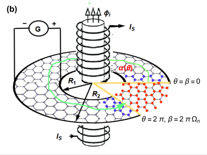
Figure 1: (color online) (a): Graphene quantum rings after Volterra construction of the inner radius $R_{1}$ and the outer radius $R_{2}$ contacted by two electrodes (thick black circles). (b): Unfolded plane of lattice where a wedge of angle $n\pi/3$ is removed, here $n=1$. $\alpha(\theta)$ is a closed path around the cone. We rescaled the angle $\beta$ of the unfolded plane to $\theta=\frac{\beta}{\Omega_{n}}$ with the wedge disclination $\Omega_{n}=1-\frac{n}{6}$. The carbon atoms of the removed sector are indicated by red balls, those which remain after the cups are represented by blue balls.

To study the above system we introduce the following Hamiltonian

$$H_{\tau}=v_{F}(\tau\pi_{x}\sigma_{x}+\pi_{y}\sigma_{y})+U(r)\mathbb{I}+\tau\Delta(r)\sigma_{z}$$ (1)

where $v_{F}=10^{6}$ m/s is the Fermi velocity, $\tau=1(-1)$ refers to the valley $K(K^{{}^{\prime}})$, $\sigma_{i}$ ($i$= $x$, $y$, $z$) are Pauli matrices in the basis of the two sublattices of $A$ and $B$ atoms, $\pi_{i}=p_{i}+eA_{i}$ are the conjugate momentum components. The involved vector potential of a solenoid is chosen in the symmetric gauge

$$\vec{A}=\frac{\hbar\Phi}{\Omega_{n}e\Phi_{0}r^{2}}(-y,x)$$ (2)

such that the wedge disclination is described by $\Omega_{n}=1-\frac{n}{6}$ [18] and $n=0,\pm 1,\pm 2$ is its associated index, with $\Phi$ is the solenoid flux and its unit $\Phi_{0}=\frac{h}{e}$. It is convenient for our task to fix the potential and gap as

$$U(r)=\left\{\begin{array}[]{ll}0,&\ \ \hbox{$R_{1}<r<R_{2}$}\\ -\hbar v_{F}V_{\infty},&\ \ \hbox{otherwise}\\ \end{array}\right.$$ (5)

$$\Delta(r)=\left\{\begin{array}[]{ll}\Delta,&\ \ \hbox{$R_{1}<r<R_{2}$}\\ 0,&\ \ \hbox{otherwise}.\\ \end{array}\right.$$ (8)

The geometry of Fig. 1 suggests to work with the polar coordinates $(r,\theta)$. Then, one can map the Hamiltonian (1) as

$$H=\begin{pmatrix}V_{+}&\partial_{-}\\ \partial_{+}&V_{-}\end{pmatrix}$$ (9)

where we have set the potentials

$$V_{\pm}(r)=U(r)\pm\tau\Delta(r)$$ (10)

and introduced the operators

$$\partial_{\pm}=-i\hbar\nu_{F}e^{\pm i\tau\theta}\left(\tau\dfrac{\partial}{\partial r}\pm\frac{i}{r}\dfrac{\partial}{\partial\theta}\mp\frac{\Phi_{i}}{\Omega_{n}r}\right)$$ (11)

with the dimensionless flux $\Phi_{i}=\frac{\Phi}{\Phi_{0}}$. The circular symmetry of the quantum rings ensures the conservation of the total angular momentum $J_{z}=L_{z}+\tau\hbar\frac{\sigma_{z}}{2}$, i.e. $[H,J_{z}]=0$. Thus, the eigenspinors can be expressed in terms of angular and radial components as

$$\Psi^{\tau}_{m}(r,\theta)=\begin{pmatrix}\chi^{\tau}_{A}(r)\psi^{+}_{m}(\theta)\\ \chi^{\tau}_{B}(r)\psi^{-}_{m\pm{\tau}}(\theta)\end{pmatrix}$$ (12)

such that the eigenstates of $J_{z}$ are given by

$$\psi_{m}^{+}(\theta)=\frac{e^{im\theta}}{\sqrt{2\pi}}\begin{pmatrix}1\\ 0\end{pmatrix},\quad\psi_{m\pm\tau}^{-}(\theta)=\frac{e^{i(m\pm{\tau})\theta}}{\sqrt{2\pi}}\begin{pmatrix}0\\ 1\end{pmatrix}$$ (13)

where $m=\pm 1,\pm 2,\cdots$, is the integer-value angular momentum quantum number, and the subscripts $A(B)$ labels the upper (lower) spinor element.

Now, we solve the Dirac equation in the three regions shown in Fig. 1b

$$H_{\tau}\Psi^{\tau}_{m}(r,\theta)=E_{\tau}\Psi^{\tau}_{m}(r,\theta)$$ (14)

which gives rise to

$$\left(\tau\dfrac{\partial}{\partial r}+\frac{m+\tau}{r}+\frac{\Phi_{i}}{\Omega_{n}r}\right)\chi^{\tau}_{B}(r)=i\kappa_{+}^{\tau}\chi^{\tau}_{A}(r)$$ (15)

$$\left(\tau\dfrac{\partial}{\partial r}-\frac{m}{r}-\frac{\Phi_{i}}{\Omega_{n}r}\right)\chi^{\tau}_{A}(r)=i\kappa_{-}^{\tau}\chi^{\tau}_{B}(r)$$ (16)

where we have defined $\kappa^{\tau}_{\pm}=\epsilon_{\tau}-V\pm\tau\delta$ and the dimensionless parameters are used $\epsilon_{\tau}=\frac{E_{\tau}}{\hbar v_{F}}$, $V=\frac{U}{\hbar v_{F}}$, $\delta=\frac{\Delta}{\hbar v_{F}}$. We proceed further by deriving a second differential equation for $\chi^{\tau}_{A}(r)$

$$\left(r^{2}\frac{\partial^{2}}{\partial r^{2}}+r\dfrac{\partial}{\partial r}+r^{2}k^{2}-(m+\frac{\Phi_{i}}{\Omega_{n}})^{2}\right)\chi^{\tau}_{A}(r)=0$$ (17)

with the parameter

$$k=\sqrt{\left|(\epsilon_{\tau}-V_{i})^{2}-\delta^{2}\right|}.$$ (18)

Under the variable change $\rho=kr$ we obtain

$$\left(\rho^{2}\frac{\partial^{2}}{\partial\rho^{2}}+\rho\dfrac{\partial}{\partial\rho}+\rho^{2}-(m+\frac{\Phi_{i}}{\Omega_{n}})^{2}\right)\chi^{\tau}_{A}(\rho)=0$$ (19)

which has the Hankel functions $H^{\pm}_{\nu}(kr)$ as general solution associated to the quantum number

$$\nu=m+\frac{\Phi_{i}}{\Omega_{n}}.$$ (20)

Consequently, the radial components $\chi^{\tau}_{m}=(\chi^{\tau}_{A},\chi^{\tau}_{B})^{T}$ for the incoming and outgoing waves are given by

$$\chi^{{\tau}(inc)}_{\nu}(r)=\begin{pmatrix}H_{\nu}^{-}(kr)\\ iH^{-}_{\nu+\tau}(kr)\end{pmatrix}$$ (21)

$$\chi^{{\tau}(out)}_{m}(r)=\begin{pmatrix}H^{+}_{\nu}(kr)\\ iH^{+}_{\nu+\tau}(kr)\end{pmatrix}.$$ (22)

Now we consider the solutions of each region. Indeed, in the disk area ($R_{1}<r<R_{2}$), we have $U(r)=0$, $\Delta(r)\neq 0$ and the electron-doping case $E_{\tau}>U(r)$. Then the solution can be represented as

$$\chi^{\tau(2)}_{\nu}(r)=a^{\tau}\begin{pmatrix}H^{-}_{\nu}(kr)\\ iH^{-}_{\nu+\tau}(kr)\end{pmatrix}+b^{\tau}\begin{pmatrix}H^{+}_{\nu}(kr)\\ iH^{+}_{\nu+\tau}(kr)\end{pmatrix}$$ (23)

with $a^{\tau}$, $b^{\tau}$ being arbitrary constants and from (18) we derive

$$k=\sqrt{\left|\epsilon_{\tau}^{2}-\delta^{2}\right|}$$ (24)

For the region $r<R_{1}$ (the inner disk) and $r>R_{2}$ (the outer disk), we have $U(r)=U_{\infty},\Delta(r)=0$. As a result, we get the solutions for $r<R_{1}$

$$\chi^{\tau(1)}_{\nu}(r)=\begin{pmatrix}H^{-}_{\nu}(k_{\infty}r)\\ iH^{-}_{\nu+\tau}(k_{\infty}r)\end{pmatrix}+r^{\tau}_{\nu}\begin{pmatrix}H^{+}_{\nu}(k_{\infty}r)\\ iH^{+}_{\nu+\tau}(k_{\infty}r)\end{pmatrix}$$ (25)

and $r>R_{2}$

$$\chi^{\tau(3)}_{\nu}(r)=t^{\tau}_{\nu}\begin{pmatrix}H^{-}_{\nu}(k_{\infty}r)\\ iH^{-}_{\nu+\tau}(k_{\infty}r)\end{pmatrix}$$ (26)

with (18) goes to

$$k_{\infty}=\epsilon_{\tau}+V_{\infty}\longrightarrow\pm\infty.$$ (27)

Here $r^{\tau}_{\nu}$ and $t^{\tau}_{\nu}$ are the reflection and transmission coefficients, respectively. For the need we recall the useful formula of the Hankel functions

$$H^{\pm}_{\nu+\tau}(rk)=\pm iH^{\pm}_{\nu}(rk),\quad H^{\pm}_{\nu}(rk)=[H^{\mp}_{\nu}(rk)]^{*}.$$ (28)

III Transport properties

We compute the transmission probability, conductance and Fano factor associated to our system. For this, we consider the limit of a highly doped lead $k_{\infty}r\gg 1$ to approximate the asymptotic behavior of the Hankel functions for large arguments as

$$H^{(\pm)}_{\nu}(\rho)\approx(2/\pi\rho)^{\frac{1}{2}}e^{\pm i(\rho-\nu\frac{\pi}{2}-\frac{\pi}{4})}.$$ (29)

As consequence, (25) reduce to

$$\chi^{\tau(1)}_{\nu}=\frac{e^{+ik_{\infty}r}}{\sqrt{r}}\begin{pmatrix}1\\ 1\end{pmatrix}+r^{\tau}_{\nu}\frac{e^{-ik_{\infty}r}}{\sqrt{r}}\begin{pmatrix}1\\ -1\end{pmatrix}$$ (30)

as well as (26)

$$\chi^{\tau(3)}_{\nu}=t^{\tau}_{\nu}\frac{e^{+ik_{\infty}r}}{\sqrt{r}}\begin{pmatrix}1\\ 1\end{pmatrix}.$$ (31)

Now we use the continuity of wave functions at the edges of three regions

$$\chi^{\tau(1)}_{\nu}(R_{1})=\chi^{\tau(2)}_{\nu}(R_{1})$$ (32)

$$\chi^{\tau(2)}_{\nu}(R_{2})=\chi^{\tau(3)}_{\nu}(R_{2})$$ (33)

to determine the transmission coefficient for the $\nu^{th}$ mode

$$t^{\tau}_{\nu}=\frac{4}{\pi k\sqrt{R_{1}R_{2}}}\frac{e^{+ik_{\infty}(R_{1}-R_{2})}}{\Gamma_{\nu}^{-\tau}+i\Gamma_{\nu}^{+\tau}}.$$ (34)

Therefore, the transmission probability can be obtained from $T^{\tau}_{\nu}=|t^{\tau}_{\nu}|^{2}$ as

$$T^{\tau}_{\nu}=\frac{16}{\pi^{2}(kR_{1})(kR_{2})}\frac{1}{(\Gamma_{\nu}^{-{\tau}})^{2}+(\Gamma_{\nu}^{+{\tau}})^{2}}$$ (35)

where we have defined the quantities

$$\Gamma_{\nu}^{+{\tau}} =$$ (36)

$$\operatorname{Im}\left[H_{\nu}^{-}(kR_{1})H_{\nu}^{+}(kR_{2})+H_{\nu+{\tau}}^{-}(kR_{1})H_{\nu+{\tau}}^{+}(kR_{2})\right]$$

$$\Gamma_{\nu}^{-{\tau}} =$$ (37)

$$\operatorname{Im}\left[H_{\nu}^{-}(kR_{1})H_{\nu+{\tau}}^{+}(kR_{2})-H_{\nu+{\tau}}^{-}(kR_{1})H_{\nu}^{+}(kR_{2})\right].$$

Recall that the wedge index $n$ is included in the quantum number $\nu$ given in (20). As a result, the wedge will affect the transmission associated to our system.

At this level we compute two interesting physical quantities related the transmission. Indeed, the conductance can be calculated within the Landauer–Büttiker formalism in the linear-response regime [19, 20]. It is provided by the relation

$$G=g_{0}\sum_{\tau=\pm 1,\nu}T^{\tau}_{\nu}$$ (38)

where $g_{0}=\frac{4e^{2}}{h}$, with 4 accounting for spin and valley degeneracy in the graphene. Here summation is over the valley index $\tau$ and quantum number $\nu$.

As for the Fano factor quantifying the power of shot noise for graphene, it is given by the summation over all modes. This is

$$\mathcal{F}^{\tau}=\frac{\sum_{\nu}\left[T^{\tau}_{\nu}\left(1-T^{\tau}_{\nu}\right)\right]}{\sum_{\nu}T^{\tau}_{\nu}}.$$ (39)

The results obtained so far will numerically be analyzed under suitable choices of the physical parameters. With this we can characterize the influence of wedge disclination on the transport properties of our system described schematically in Fig. 1.

IV Results and discussions

Figure 2: (color online) The transmission $T_{\nu}$ $(m=1,2,3)$ as a function of the doping $k_{F}R_{1}$ for a radii ratio $R_{2}/R_{1}=5$, $\Phi_{i}=\frac{1}{2}$ (solid line) and $\Phi_{i}=\frac{3}{2}$ (dashed line), with $n=0$ (blue line), $n=1$ (red line), $n=2$ (magenta line), $n=-1$ (green line), $n=-2$ (orange line). (a${}_{\text{m}}$): $K(\tau=+1)$ and $R_{1}\delta=0$, (b${}_{\text{m}}$): $K^{\prime}(\tau=-1)$ and $R_{1}\delta=0$, (c${}_{\text{m}}$): $K(\tau=+1)$ and $R_{1}\delta=2$, (d${}_{\text{m}}$): $K^{\prime}(\tau=-1)$ and $R_{1}\delta=2$.

We numerically study the transmission $T_{\nu}$ $(m=1,2,3)$, the conductance $G$ and Fano factor $\mathcal{F}$ of the Corbino disk in graphene obtained by creating a gap in the disk area ($R_{1}<r<R_{2}$). Indeed, Fig. 2 represents the transmission as function of doping $k_{F}R_{1}$ for the two valleys $K(\tau=+1)$ and $K^{\prime}(\tau=-1)$ with two values of energy gap $R_{1}\delta=0,2$, magnetic flux $\Phi_{i}=\frac{1}{2},\frac{3}{2}$ and the wedge index $n=0,\pm 1,\pm 2$. Knowing that $n=0$ corresponds to an isolated in the defect-free case, $n=1$ to an isolated pentagon defect, $n=2$ to an isolated square defect, $(n=-1)$ to an isolated heptagon defect and $(n=-2)$ corresponds to an isolated octagon defect. One sees that more the flux magnetic is increased, the more the transmission is decreasing. The transmission of $K^{\prime}(\tau=-1)$ is greater than that for $K(\tau=+1)$. We observe a suppression of the tunneling and the electrons are totally reflected for $k_{F}R_{1}=R_{1}\delta$, which depends on whether the back-scattering phenomenon is canceled in the presence of energy gap $\delta$ or not. This is in agreement with our previous results obtained in [16]. The transmission changes compared to the defect free case $n=0$ knowing that the transmission for a negative value of $n$ is greater than that for a positive value of $n$. We notice that the difference in the transmission between $n=0$ and $n\neq 0$ becomes very important in the presence of magnetic flux $\Phi_{i}$. We observe that the transmission strongly depends on the valley and magnetic flux knowing that the configuration which can have a full transmission (Klein tunneling) is $(m=1,\tau=-1,\Phi_{i}=\frac{1}{2})$, see Figs. 2(b${}_{\text{1}}$,d${}_{\text{1}}$).

Figure 3: (color online) The transmission $T_{\nu}$ $(m=1,2,3)$ as a function of the radii ratio $R_{2}/R_{1}$ for the doping $k_{F}R_{1}=0.1$, $\Phi_{i}=\frac{1}{2}$, $K(\tau=+1)$ (solid line) and $K^{\prime}(\tau=-1)$ (dashed line). $n=0$ (blue line), $n=1$ (red line), $n=2$ (magenta line), $n=-1$ (green line), $n=-2$ (orange line). (a,b,c): $R_{1}\delta=0$, (d,e,f): $R_{1}\delta=2$.

Fig. 3 shows the transmission $T_{\nu}$ $(m=1,2,3)$ as a function of the radii ratio $R_{2}/R_{1}$ for the valleys $K(\tau=+1)$ and $K^{\prime}(\tau=-1)$, two values of energy gap $R_{1}\delta=0$ (Figs. 2(a,b,c)) and $R_{1}\delta=2$ (Figs. 3(d,e,f)), magnetic flux $\Phi_{i}=\frac{1}{2},\frac{3}{2}$ and $n=0,\pm 1,\pm 2$. For $R_{1}\delta=0$, the transmission decreases exponentially whatever the value of $n$ and the valley index $\tau=\pm 1$. For $R_{1}\delta=2$, we observe oscillations that become more and more of distinct peaks for $K^{\prime}(\tau=-1)$ (Figs. 3(d,e,f)). We have a full transmission (Klein tunneling) for $R_{1}\delta=0$, $\tau=-1$ and $n=-2$. We notice that the amplitude of these oscillations decreases when the parameter of the radii ratio $R_{2}/R_{1}$ is increased and depends on the value of the disclination effect $n$ knowing that its smallest value corresponds to the case where $n=-2$ the octagon defect. Both Figs. 2 and 3 show that the transmission is reduced if the value of the angular momentum $\nu$ is increased.

Figure 4: (color online) The Fano factor $\mathcal{F}$ as a function of the doping $k_{F}R_{1}$ for the radii ratio $R_{2}/R_{1}=5$, $R_{1}\delta=1$ (solid line) and $R_{1}\delta=3$ (dashed line). $n=0$ (blue line), $n=1$ (red line), $n=2$ (magenta line), $n=-1$ (green line), $n=-2$ (orange line). (a,b,c): $K(\tau=+1)$, (d,e,f): $K^{\prime}(\tau=-1)$. (a,d): $\Phi_{i}=\frac{1}{2}$, (b,e): $\Phi_{i}=\frac{3}{2}$, (c,f): $\Phi_{i}=\frac{5}{2}$.

In Fig. 4, we report the Fano factor as a function of the doping $k_{F}R_{1}$ for the radii ratio $R_{2}/R_{1}=5$, energy gap $R_{1}\delta=1$ (solid line) and $R_{1}\delta=3$ (dashed line), $n=0,\pm 1,\pm 2$ and magnetic flux $\Phi_{i}=\frac{1}{2},\frac{3}{2},\frac{5}{2}$. We first observe that $\mathcal{F}$ is independent of the valley $K(\tau=+1)$ or $K^{\prime}(\tau=-1)$. Figs. 4(a,d) are for $\Phi_{i}=1/2$ where we observe intense peaks at the point $k_{F}R_{1}=R_{1}\delta$, then the curves follow an oscillatory process for high doping just for the case of a square defect $n=2$. For $n=0,\pm 1,-2$ there exists a double identical peaks of average intensity at $\mathcal{F}=0.28$. We stress that the intensity of peaks is independent of the energy gap $R_{1}\delta$. Figs. 4(b,c,e,f) are for $\Phi_{i}=\frac{3}{2},\frac{5}{2}$, we observe intense peaks at the points $k_{F}R_{1}=R_{1}\delta$ for $n\neq 0$ whose maximum intensity value varies from one case to another. Obviously the case where $n=0$ free defect remains unchanged.

Figure 5: (color online) The Fano factor $\mathcal{F}$ as a function of the magnetic flux $\Phi_{i}$ for the doping $k_{F}R_{1}=0.2$ and the valley $K(\tau=+1)$. (a,b,c,d,e): $R_{2}/R_{1}=5$, $R_{1}\delta=0$ (blue line), $R_{1}\delta=0.4$ (red line), $0.8$ (green line). (a): $n=0$, (b): $n=1$, (c): $n=2$, (d): $n=-1$, (e): $n=-2$. (f): $R_{1}\delta=0.4$, $R_{2}/R_{1}=5$ (solid line ), $R_{2}/R_{1}=6$ (dashed line ), $n=0$ (blue line), $n=1$ (red line), $n=2$ (magenta line), $n=-1$ (green line), $n=-2$ (orange line).

Fig. 5 represents the Fano factor $\mathcal{F}$ as function the magnetic flux $\Phi_{i}$ for a low doping $k_{F}R_{1}=0.2$. We observe that $\mathcal{F}$ shows a periodic oscillation and its amplitude depends on both $R_{1}\delta$ and $R_{2}/R_{1}$ because its decreases with the increasing of them. It is interesting to note that the period of these oscillations depends on $n$. Indeed, the maximal period of the oscillations corresponds to the octagon defect $n=-2$ while the minimal one corresponds to square defect $n=2$. Then it is clearly seen that the wedge index $n$ acts by changing the period of the oscillations of $\mathcal{F}$.

Fig. 6 shows the conductance $G[g_{0}]$ as a function of the doping $k_{F}R_{1}$ for $\Phi_{i}=\frac{1}{2},\frac{3}{2}$. It can be written in the approximate form

$$G\approx 2g_{0}R_{1}\sqrt{|k_{F}^{2}-\delta^{2}|}+G_{min}(n,\Phi_{i})$$ (40)

where $G_{min}(n,\Phi_{i})$ is the minimum value of $G$, which is depending on $n$ (disclination effect) and $\Phi_{i}$ (magnetic flux). (40) is in agreement with the result that we previously found [16]. $G$ increases when the doping increases and for zero doping ($k_{F}R_{1}=0$), it increases by increasing the energy gap. It is clearly seen that $G$ takes a minimal value $G_{min}(n,\Phi_{i})$ for $k_{F}R_{1}=R_{1}\delta$. We observe that adding an energy gap $R_{1}\delta$ implies an appearance of a singularity where the conductance becomes minimal for the doping case $k_{F}R_{1}=R_{1}\delta$. The conductance for a zero doping $G(k_{F}R_{1}=0)$ is increased when the value of $R_{1}\delta$ increases.

Figure 6: (color online) The conductance $G[g_{0}]$ as a function of the doping $k_{F}R_{1}$ for the radii ratio $R_{2}/R_{1}=5$ with $n=0$ (blue line), $n=1$ (red line), $n=2$ (magenta line), $n=-1$ (green line) and $n=-2$ (orange line). Inset presents a zoom-in for low doping $k_{F}R_{1}<0.8$. (a,c): $R_{1}\delta=0.5$, (b,d): $R_{1}\delta=1$, (a,b): $\Phi_{i}=\frac{1}{2}$, (c,d): $\Phi_{i}=\frac{3}{2}$.

Fig. 7 shows contour plot of the conductance $G[g_{0}]$ as a function of the doping $k_{F}R_{1}$ and the energy gap $R_{1}\delta$ with (a): $R_{2}/R_{1}=5$ and (b): $R_{2}/R_{1}=7.5$ for free defect $n=0$. We observe that the conductance for zero doping is proportional to the energy gap and all points where the conductance is minimum are reduced for $R_{2}\gg R_{1}$ (surface hatched by the color black).

Figure 7: (color online) Contour plot of the conductance $G[g_{0}]$ as a function of the doping $k_{F}R_{1}$ and energy gap $R_{1}\delta$ for free defect $n=0$. (a): $R_{2}/R_{1}=5$, (b): $R_{2}/R_{1}=7.5$.

To study the effect of wedge index $n=0,\pm 1,\pm 2$ and magnetic flux $\Phi_{i}=\frac{1}{2},\frac{3}{2}$ on $G_{min}(n,\Phi_{i})$, in Fig. 8 we show the conductance as a function of the doping $k_{F}R_{1}$. To analyze such case, let us show some illustrations under suitable choices.

1. The minimal value of the conductance $G_{min}(n,\Phi_{i})$

   • $G_{min}(n,\frac{1}{2})$:

     $$G_{min}(0)=1.31g_{0},\ G_{min}(1)=1.22g_{0},\ G_{min}(2)=1.24g_{0}$$

     $$G_{min}(-1)=1.26g_{0},\ G_{min}(-2)=1.20g_{0}$$

   • $G_{min}(n,\frac{3}{2})$:

     $$G_{min}(0)=1.31g_{0},\ G_{min}(1)=1.17g_{0},\ G_{min}(2)=1.24g_{0}$$

     $$G_{min}(-1)=1.21g_{0},\ G_{min}(-2)=1.19g_{0}$$

2. The initial value of the conductance $G_{int}(k_{F}R_{1}=0,n,\Phi_{i})$

   • $G_{int}(k_{F}R_{1}=0,n,\frac{1}{2})$

     $$G_{int}(0)=1.78g_{0},\ G_{int}(1)=1.82g_{0},\ G_{int}(2)=1.81g_{0}$$

     $$G_{int}(-1)=1.80g_{0},\ G_{int}(-2)=1.83g_{0}$$

   • $G_{int}(k_{F}R_{1}=0,n,\frac{3}{2})$

     $$G_{int}(n0)=1.78g_{0},\ G_{int}(1)=1.84g_{0},\ G_{int}(2)=1.81g_{0}$$

     $$G_{int}(-1)=1.82g_{0},\ G_{int}(-2)=1.83g_{0}$$

Figure 8: (color online) The conductance $G[g_{0}]$ as a function of the doping $k_{F}R_{1}$ for $R_{2}/R_{1}=5$ and $R_{1}\delta=0.5$ with $n=0$ (blue line), $n=1$ (red line), $n=2$ (magenta line), $n=-1$ (green line) and $n=-2$ (orange line). (a): $\Phi_{i}=\frac{1}{2}$, (b): $\Phi_{i}=\frac{3}{2}$.

In Fig. 9, we show the conductance $G[g_{0}]$ as a function of the magnetic flux $\Phi_{i}$. First we prove the approximate expressions of the transmission and the conductance for zero doping $k_{F}R_{1}\to 0$. Indeed, for zero doping limit the transmission for the Corbino disk in undoped graphene (35) can be simplified to [21]

$$T^{\tau}_{\nu}=\frac{1}{\cosh^{2}[\ln(R_{2}/R_{1})(\nu+\frac{\Phi_{i}}{\Omega_{n}})]}$$ (41)

and then the corresponding conductance (38) becomes

$$G(\Phi_{i})=\sum^{\infty}_{j=0}G_{j}\cos\left(\frac{2\pi\Phi_{i}}{\Omega_{n}}\right)$$ (42)

where the coefficients are given by

$$G_{0}=\frac{2g_{0}}{\ln(R_{2}/R_{1})}$$ (43)

$$G_{j}=\frac{4\pi^{2}(-1)^{j}jg_{0}}{\ln(R_{2}/R_{1})^{2}\sinh[\pi^{2}j/\ln(R_{2}/R_{1})]}.$$ (44)

(42) shows the explicit dependence of the conductance $G[g_{0}]$ on the magnetic flux $\Phi_{i}$ and also the magnitude $\Omega_{n}$ as its period. It clearly seen that the conductance oscillations are of Aharonov-Bohm types whose amplitude depends on $R_{1}\delta$ and $R_{2}/R_{1}$. This shows a good agreement with our previous results [16]. The amplitude of $G\left(\Phi_{i}\right)$ oscillations reduces by increasing $R_{1}\delta$ or decreasing $R_{2}/R_{1}$. We notice that a perfectly periodic functional dependence of $G[g_{0}]$ on $\Phi_{i}$ with an average value $G_{0}$ equal to the pseudo-diffusion conductance such that the greatest value corresponds to octagon defect $n=-2$ and the smallest one is for square defect $n=2$. These symmetry properties have the consequence that the conductance (42) is symmetric if the flux is reversed, i.e. $G(-\Phi_{i})=G(\Phi_{i})$.

Figure 9: (color online) The conductance $G[g_{0}]$ as a function of the magnetic flux $\Phi_{i}$ for $k_{F}R_{1}=0.1$. (a,b,c,d,e): $R_{2}/R_{1}=5$ with $R_{1}\delta=0$ (blue line), $0.15$ (red line), $0.2$ (magenta line), $0.25$ (green line), $0.3$ (orange line). (a): $n=0$, (b): $n=1$, (c): $n=-1$, (d): $n=2$, (e): $n=-2$. (f): $R_{1}\delta=0$, $R_{2}/R_{1}=5$ (solid line), $R_{2}/R_{1}=7.5$ (dashed line) with $n=1$ (red line), $n=2$ (magenta line), $n=-1$ (green line), $n=-2$ (orange line).

We study the magnitude of conductance oscillations $\Delta G$. It is defined as the difference between $G(1/2)$ and $G(0)$

$$\Delta G=G(1/2)-G(0).$$ (45)

Fig. 10 shows the magnitude of the conductance oscillations $\Delta G$ as a function of the doping $k_{F}R_{1}$ for $n=0,\pm 1,\pm 2$, $R_{2}/R_{1}=5,7.5$ and $R_{1}\delta=0,2,4$. There is appearance of resonance peaks when $k_{F}R_{1}$ is close to $R_{1}\delta$ as noticed in [16]. We point out that the frequency of these resonance peaks depends only on $R_{1}\delta$ knowing that it increases with its increase. It is interesting to notice that $n$ changes the amplitude of the resonance peak for $k_{F}R_{1}=R_{1}\delta$. A sharp resonance is obtained in the case of octagon defect $n=-2$.

Figure 10: (color online) The magnitude of the conductance oscillations $\Delta G$ as a function of the doping $k_{F}R_{1}$ for three values $R_{1}\delta=0$ (blue line), $2$ (red line) and $4$ (green line). (a,b,c,d,e): $R_{2}/R_{1}=5$, (f,g.h,i): $R_{2}/R_{1}=7.5$. (a): $n=0$, (b,i): $n=1$, (c,h): $n=-1$, (d,g): $n=2$, (e,f): $n=-2$.

V Conclusion

We have studied gapped graphene in the shape of a quantum ring of inner radius $R_{1}$ and outer radius $R_{2}$ subjected to a magnetic flux $\Phi_{i}$ with a topological defect created using a procedure known as the Volterra process [17]. Taking into account the advantage of the geometry of the Corbino disk in graphene, we have solved the corresponding stationary Dirac equation and obtained analytically the energy spectrum solutions in the three regions. We have determined the transmission probability of an electron crossing the Corbino disk in graphene as well as the conductance $G$ and Fano factor $\mathcal{F}$.

Our numerical results were exposed in terms of the radii ratio $R_{2}/R_{1}$, magnetic flux $\Phi_{i}$, energy gap $R_{1}\delta$ and wedge disclination $n$. We have demonstrated the influence of $n$ on the transmission probability. For positive $n$ the transmission probability decreases with growing of $n$, while for $n$ negative it increases compared to gapped-graphene with $n=0$. We have showed that $n$ modifies the period of Fano factor oscillations and allows to intensive peaks at some points. Additionally, it was found that the conductance of the Corbino disk (as a function of magnetic flux piercing the disk) presents periodic oscillations of the Aharonov-Bohm type where its period depends on $n$. We have seen that the energy gap, the radii ratio and $n$ can change the characteristics of the oscillations of $G(\Phi_{i})$ and the resonances of $\Delta G$ when the doping $k_{F}R_{1}$ is close to the value of $R_{1}\delta$.

References

• [1] R. A. Webb, S. Washburn, C. P. Umbach, and R. B. Laibowitz, Phys. Rev. Lett. 54, 2696 (1985).
• [2] D. Mailly, C. Chapelier, and A. Benoit, Phys. Rev. Lett. 70, 2020 (1993).
• [3] P. Földi, M. G. Benedict, O. Kálmán, and F. M. Peeters, Phys. Rev. B 80, 165303 (2009).
• [4] Y. Aharonov and D. Bohm, Phys. Rev. 115, 485 (1959).
• [5] J. Schelter, D. Bohr, and B. Trauzettel, Phys. Rev. B 81, 195441 (2010).
• [6] S. Russo, J. B. Oostinga, D. Wehenkel, H. B. Heersche, S. S. Sobhani, L. M. K. Vandersypen, and A. F. Morpurgo, Phys. Rev. B 77, 085413 (2008).
• [7] M. Huefner, F. Molitor, A. Jacobsen, A. Pioda, C. Stampfer, K. Ensslin, and T. Ihn, Phys. Status Solidi b 246, 2756 (2009).
• [8] J. Schelter, P. Recher, and B. Trauzettel, Solid State Commun. 152, 1411 (2012).
• [9] M. Zarenia, J. M. Pereira, Jr., F. M. Peeters, and G. A. Farias, Nano Lett. 9, 4088 (2009).
• [10] Y. Zhao, P. Cadden-Zimansky, F. Ghahari, and P. Kim, Phys. Rev. Lett 108, 106804 (2012).
• [11] E. C. Peters, A. J. M. Giesbers, M. Burghard, and K. Kern, Appl. Phys. Lett. 104, 203109 (2014).
• [12] A. Rycerz, Phys. Rev. B 81, 121404(R) (2010).
• [13] Z. Khatibi, H. Rostami, and R. Asgari, Phys. Rev. B 88, 195426 (2013).
• [14] B. Abdollahipour and E. Moomivand, Physica E 86, 204 (2017).
• [15] A. Rycerz and D. Suszalski, Phys. Rev. B 101, 245429 (2020).
• [16] A. Babe Cheikh, A. Bouhlal, A. Jellal, and E. H. Atmani, Phys. Scr. 96, 125863 (2021).
• [17] Cludio Furtado, Bruno G. C. da Cunhaa, Fernando Moraesa, E. R. Bezerra de Mello, and V. B. Bezzerrab, Phys. Lett. A 195, 90 (1994).
• [18] Yu.V. Nazarov and Ya. M. Blanter, Quantum Transport: Introduction to Nanoscience (Cambridge University Press, Cambridge, UK, 2009, Chap. 1).
• [19] Rolf Landauer, Philos. Mag. 21, 863 (1970).
• [20] M. Büttiker, Phys. Rev. B 46, 12485 (1992).
• [21] M. Büttiker, Y. Imry, R. Landauer, and S. Pinhas, Phys. Rev. B 31, 6207 (1985).